Time Series - STAT - EPFL
Time Series - STAT - EPFL
Time Series - STAT - EPFL

Create successful ePaper yourself
Turn your PDF publications into a flip-book with our unique Google optimized e-Paper software.
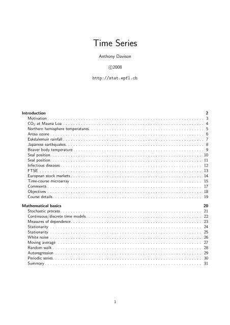
<strong>Time</strong> <strong>Series</strong><br />
Anthony Davison<br />
c○2008<br />
http://stat.epfl.ch<br />
Introduction 2<br />
Motivation . . . . . . . . . . . . . . . . . . . . . . . . . . . . . . . . . . . . . . . . . . . . . . . . . . . . . . . . . . . . . 3<br />
CO 2 at Mauna Loa . . . . . . . . . . . . . . . . . . . . . . . . . . . . . . . . . . . . . . . . . . . . . . . . . . . . . . . 4<br />
Northern hemisphere temperatures. . . . . . . . . . . . . . . . . . . . . . . . . . . . . . . . . . . . . . . . . . . . . 5<br />
Arosa ozone . . . . . . . . . . . . . . . . . . . . . . . . . . . . . . . . . . . . . . . . . . . . . . . . . . . . . . . . . . . . 6<br />
Eskdalemuir rainfall . . . . . . . . . . . . . . . . . . . . . . . . . . . . . . . . . . . . . . . . . . . . . . . . . . . . . . . 7<br />
Japanese earthquakes. . . . . . . . . . . . . . . . . . . . . . . . . . . . . . . . . . . . . . . . . . . . . . . . . . . . . . 8<br />
Beaver body temperature . . . . . . . . . . . . . . . . . . . . . . . . . . . . . . . . . . . . . . . . . . . . . . . . . . . 9<br />
Seal position. . . . . . . . . . . . . . . . . . . . . . . . . . . . . . . . . . . . . . . . . . . . . . . . . . . . . . . . . . . 10<br />
Seal position. . . . . . . . . . . . . . . . . . . . . . . . . . . . . . . . . . . . . . . . . . . . . . . . . . . . . . . . . . . 11<br />
Infectious diseases . . . . . . . . . . . . . . . . . . . . . . . . . . . . . . . . . . . . . . . . . . . . . . . . . . . . . . . 12<br />
FTSE . . . . . . . . . . . . . . . . . . . . . . . . . . . . . . . . . . . . . . . . . . . . . . . . . . . . . . . . . . . . . . . 13<br />
European stock markets . . . . . . . . . . . . . . . . . . . . . . . . . . . . . . . . . . . . . . . . . . . . . . . . . . . 14<br />
<strong>Time</strong>-course microarray . . . . . . . . . . . . . . . . . . . . . . . . . . . . . . . . . . . . . . . . . . . . . . . . . . . 15<br />
Comments . . . . . . . . . . . . . . . . . . . . . . . . . . . . . . . . . . . . . . . . . . . . . . . . . . . . . . . . . . . . 17<br />
Objectives . . . . . . . . . . . . . . . . . . . . . . . . . . . . . . . . . . . . . . . . . . . . . . . . . . . . . . . . . . . . 18<br />
Course details. . . . . . . . . . . . . . . . . . . . . . . . . . . . . . . . . . . . . . . . . . . . . . . . . . . . . . . . . . 19<br />
Mathematical basics 20<br />
Stochastic process. . . . . . . . . . . . . . . . . . . . . . . . . . . . . . . . . . . . . . . . . . . . . . . . . . . . . . . 21<br />
Continuous/discrete time models. . . . . . . . . . . . . . . . . . . . . . . . . . . . . . . . . . . . . . . . . . . . . 22<br />
Measures of dependence. . . . . . . . . . . . . . . . . . . . . . . . . . . . . . . . . . . . . . . . . . . . . . . . . . . 23<br />
Stationarity . . . . . . . . . . . . . . . . . . . . . . . . . . . . . . . . . . . . . . . . . . . . . . . . . . . . . . . . . . . 24<br />
Stationarity . . . . . . . . . . . . . . . . . . . . . . . . . . . . . . . . . . . . . . . . . . . . . . . . . . . . . . . . . . . 25<br />
White noise . . . . . . . . . . . . . . . . . . . . . . . . . . . . . . . . . . . . . . . . . . . . . . . . . . . . . . . . . . . 26<br />
Moving average . . . . . . . . . . . . . . . . . . . . . . . . . . . . . . . . . . . . . . . . . . . . . . . . . . . . . . . . 27<br />
Random walk . . . . . . . . . . . . . . . . . . . . . . . . . . . . . . . . . . . . . . . . . . . . . . . . . . . . . . . . . . 28<br />
Autoregression . . . . . . . . . . . . . . . . . . . . . . . . . . . . . . . . . . . . . . . . . . . . . . . . . . . . . . . . . 29<br />
Periodic series. . . . . . . . . . . . . . . . . . . . . . . . . . . . . . . . . . . . . . . . . . . . . . . . . . . . . . . . . . 30<br />
Summary . . . . . . . . . . . . . . . . . . . . . . . . . . . . . . . . . . . . . . . . . . . . . . . . . . . . . . . . . . . . . 31<br />
1
Introduction slide 2<br />
Motivation<br />
□ In basic data analysis we make often assume that observations are independent or even<br />
independent identically distributed,<br />
X 1 ,...,X n<br />
ind<br />
∼ F 1 ,...,F n ,<br />
X 1 ,... ,X n<br />
iid ∼ N(µ,σ 2 ).<br />
□ <strong>Time</strong> series is the study of observations that arise in some order (almost always time) and which<br />
as a result are dependent.<br />
□ There are many more ways to be dependent than to be independent, and almost all data are<br />
collected in time order, so time series arise in a vast range of disciplines: economics; finance;<br />
marketing; epidemiology; biomedicine; genomics; environmental science; computer science;<br />
electrical engineering; physics; ...<br />
□ Many of these disciplines have developed special techniques for their data types, and we will only<br />
scratch the surface of them in this course, by surveying some main ideas.<br />
<strong>Time</strong> <strong>Series</strong> Autumn 2008 – slide 3<br />
CO 2 at Mauna Loa<br />
Monthly levels of carbon dioxide (ppm) at Mauna Loa (Hawaii) from March 1958 to July 2007.<br />
co2<br />
320 340 360 380<br />
1960 1970 1980 1990 2000<br />
<strong>Time</strong><br />
<strong>Time</strong> <strong>Series</strong> Autumn 2008 – slide 4<br />
2
Northern hemisphere temperatures<br />
Temperature anomaly ( ◦ C) for 0–1979 relative to 1961–1990 instrumental average.<br />
Temperature anomaly (C)<br />
−1.5 −1.0 −0.5 0.0 0.5<br />
0 500 1000 1500 2000<br />
Year (AD)<br />
<strong>Time</strong> <strong>Series</strong> Autumn 2008 – slide 5<br />
Arosa ozone<br />
Annual average and daily total atmospheric ozone measurements (in Dobson units) at Arosa.<br />
Annual average ozone (DU)<br />
300 330 360<br />
Daily ozone (DU)<br />
200 350 500<br />
1940 1950 1960 1970 1980 1990 2000<br />
<strong>Time</strong><br />
1940 1950 1960 1970 1980 1990 2000<br />
<strong>Time</strong><br />
<strong>Time</strong> <strong>Series</strong> Autumn 2008 – slide 6<br />
3
Eskdalemuir rainfall<br />
Hourly rainfall totals at Eskdalemuir, in the south of Scotland<br />
Hourly rainfall (0.1 mm)<br />
0 50 100 150<br />
1975 1976 1977 1978 1979 1980<br />
Year<br />
<strong>Time</strong> <strong>Series</strong> Autumn 2008 – slide 7<br />
Japanese earthquakes<br />
<strong>Time</strong>s and magnitudes of earthquakes with epicentre less than 100km in an offshore region west of<br />
the main Japanese island of Honshū and south of the northern island of Hokkaidō. The figure shows<br />
all 483 earthquakes of magnitude 6 or more on the Richter scale in the period 1885–1980, about 5<br />
tremors per year, in one of the most seismically active areas of Japan.<br />
Magnitude (Richter units)<br />
6.0 6.5 7.0 7.5 8.0 8.5<br />
0 5000 10000 15000 20000 25000 30000 35000<br />
Days since 1 January 1885<br />
<strong>Time</strong> <strong>Series</strong> Autumn 2008 – slide 8<br />
4
Beaver body temperature<br />
100 consecutive telemetric measurements on the body temperature of a female Canadian beaver,<br />
Castor canadensis, taken at 10-minute intervals. The animal remained in its lodge for the first 38<br />
recordings and then moved outside, at which point there was a sustained temperature rise.<br />
Body temperature (C)<br />
36.5 37.0 37.5 38.0 38.5<br />
0 20 40 60 80 100<br />
<strong>Time</strong><br />
<strong>Time</strong> <strong>Series</strong> Autumn 2008 – slide 9<br />
Seal position<br />
Hawaiian monk seals, Monachus schauinslandi, number around 1300, are endemic to the Hawaiian<br />
Islands and are the most endangered species of marine mammal that lives entirely within the<br />
jurisdiction of the United States. The species has been declining partly owing to poor juvenile survival<br />
which is evidently related to poor foraging success. Data have been collected recently on the foraging<br />
habitats, movements, and behaviors of monk seals throughout the Northwestern and main Hawaiian<br />
Islands.<br />
The central Hawaiian islands<br />
22.0<br />
Kauai<br />
Oahu<br />
21.5<br />
latitude (degrees)<br />
21.0<br />
Molokai<br />
Maui<br />
Pacific Ocean<br />
20.5<br />
−159 −158 −157 −156<br />
longitude (degrees)<br />
<strong>Time</strong> <strong>Series</strong> Autumn 2008 – slide 10<br />
5
Seal position<br />
Journey of a juvenile female (4-5 years old) Hawaiian monk seal while she foraged and occasionally<br />
hauled out ashore. She was tagged and released at the southwest corner of Molokai, and tracked from<br />
13 April 2004 through 27 July 2004, using a satellite-linked radio transmitter glued to her dorsal<br />
pelage to document geographic and vertical movements as proxies of foraging behavior.<br />
Seal’s motion between pairs of the well−determined points<br />
100<br />
northing (km)<br />
80<br />
60<br />
40<br />
240 260 280 300 320 340 360<br />
easting (km)<br />
<strong>Time</strong> <strong>Series</strong> Autumn 2008 – slide 11<br />
Infectious diseases<br />
Weekly counts of new influenza and meningococcal infections in Germany 2001–2006.<br />
Meningococcus Influenza<br />
0 20 0 1000<br />
2001 2002 2003 2004 2005 2006 2007<br />
<strong>Time</strong> <strong>Series</strong> Autumn 2008 – slide 12<br />
6
FTSE<br />
The Financial <strong>Time</strong>s Stock Exchange Index, 1991–1998.<br />
FTSE Index<br />
3000 4000 5000 6000<br />
1992 1993 1994 1995 1996 1997 1998<br />
<strong>Time</strong><br />
<strong>Time</strong> <strong>Series</strong> Autumn 2008 – slide 13<br />
European stock markets<br />
The rise of European stock markets, 1991–1998.<br />
EuStockMarkets<br />
FTSE CAC SMI DAX<br />
3000 6000 1500 3500<br />
2000 6000 2000 5000<br />
1992 1993 1994 1995 1996 1997 1998<br />
<strong>Time</strong> <strong>Series</strong> Autumn 2008 – slide 14<br />
<strong>Time</strong><br />
7
<strong>Time</strong>-course microarray<br />
Expression levels for 2771 genes/sequence tages spotted on acDNA microarray, relating to gene<br />
transcription in the immune response of Anopheline mosquitoes.<br />
<strong>Time</strong> <strong>Series</strong> Autumn 2008 – slide 15<br />
<strong>Time</strong>-course microarray<br />
A clustering of the mosquito genes based on the time courses.<br />
<strong>Time</strong> <strong>Series</strong> Autumn 2008 – slide 16<br />
8
Comments<br />
□ The measurements can be continuous (temperatures) or discrete (infectious disease counts) or a<br />
mixture (rainfall), scalar or vector (seal position)<br />
□ Mostly they are at regular intervals, but some are intermittent (quakes)<br />
□ Some are instantaneous values, others are integrals (rain)<br />
□ Some series exhibit strong trend and/or seasonality (CO 2 , infectious diseases, stock markets)<br />
□ There can be missing observations and/or possible outliers (ozone, rainfall)<br />
□ <strong>Series</strong> can be long (rainfall, temperatures) or very short (microarray)<br />
□ May be one or a few or many series<br />
□ Focus may be<br />
– a possible change in the underlying series, so the dependence is a nuisance (e.g. ozone,<br />
temperatures, beaver, microarray)<br />
– dependence/interaction within or between series (quakes, diseases, stock markets)<br />
– rare events (stock markets, rainfall, ozone)<br />
– comparison of parallel series (microarray)<br />
<strong>Time</strong> <strong>Series</strong> Autumn 2008 – slide 17<br />
Objectives<br />
Typically we have in mind one or more of the following general objectives:<br />
□ Description<br />
– Want a ‘simple’ summary of the series<br />
□ Analysis<br />
– Construct stochastic model(s), and try and answer questions with them<br />
– Model will reflect knowledge about phenomenon under study and complexity of data available<br />
– May just need to accommodate dependence as part of larger analysis<br />
□ Monitoring/Control<br />
– Blood pressure/chemical reactor temperature must be kept between x 0 and x 1<br />
– Aim to detect changes as they occur and to influence process in real time<br />
□ Forecasting<br />
– ‘What will the market do tomorrow’ ‘What will the economy do next year’<br />
– Sometimes the model is not so important (though economic models may be complex)<br />
– Often combine different models to get best forecasts (‘model averaging’)<br />
<strong>Time</strong> <strong>Series</strong> Autumn 2008 – slide 18<br />
9
Course details<br />
□ Place: MA30 (= MA A3 30)<br />
□ Lectures 8.15–10.00, Monday 29 September 2008 onwards<br />
□ Exercises 10.15–12.00, Monday 29 September 2008 onwards<br />
□ Main reference: Shumway and Stoffer (2006) <strong>Time</strong> <strong>Series</strong> Analysis and its Applications. Second<br />
edition. Springer-Verlag<br />
□ Form of exam not yet determined (probably written, may be some project component)<br />
□ Notes and exercises can be downloaded from course web page<br />
http://stat.epfl.ch/page32112.html<br />
<strong>Time</strong> <strong>Series</strong> Autumn 2008 – slide 19<br />
Mathematical basics slide 20<br />
Stochastic process<br />
Definition 1 (a) A stochastic process {Y t } t∈T with index set T is a family of random variables<br />
defined on a probability space (Ω, F,P).<br />
(b) A realisation of {Y t } is the outcome {y t } t∈T = {Y t (ω)} t∈T for some ω ∈ Ω.<br />
The index set T :<br />
□ most models have index set T = R, R + , or Z; item owing to digitisation, T cannot in practice<br />
contain a sub-interval of R, but the time step ∆ can be very small in some applications;<br />
□ (almost-)continuous time series can be thinned by subsampling at the points of a grid, or, in some<br />
cases, by integration over intervals of width ∆ (e.g. rainfall data);<br />
□ for general discussion of time series we take T = Z, so that Y t is recorded at times 0, ±1, ±2,...,<br />
and write a realisation of the process observed for a finite period as y 1 ,...,y n .<br />
□ Intermittent time series involve index sets T that are not regular grids.<br />
<strong>Time</strong> <strong>Series</strong> Autumn 2008 – slide 21<br />
10
Continuous/discrete time models<br />
Two main situations:<br />
□ available data are part of a random sequence {Y t }, for which time t takes only integer values,<br />
i.e. t ∈ Z. Thus Y t does not exist at (say) t = 0.5;<br />
□ available data are values of a random function {Y (t)} that exists for all t ∈ R (or R + ) but is<br />
only observed at a limited number of times.<br />
In some cases (e.g. rainfall, with the time unit being hours) the observed data are<br />
∫ t<br />
t−1<br />
Y (t)dt.<br />
In this case, and particularly if we will want to use different time scales, there is a good case for<br />
building a continuous-time model but estimating its parameters etc. using the cumulated/discrete<br />
time data. Otherwise conclusions made for different time scales may be incoherent.<br />
<strong>Time</strong> <strong>Series</strong> Autumn 2008 – slide 22<br />
Measures of dependence<br />
Definition 2 Let {Y t } t∈T be a stochastic process. Then<br />
(a) if E(|Y t |) < ∞, then we define the mean (or expectation) of the process to be µ t = E(Y t ). If<br />
non-constant µ t is sometimes called the trend;<br />
(b) if var(Y t ) < ∞ for all t ∈ T , then we define the (auto)covariance function of the process to be<br />
γ(s,t) = cov(Y s ,Y t ) = E {(Y s − µ s )(Y t − µ t )} , s,t ∈ T ,<br />
and the (auto)correlation function of the process to be<br />
ρ(s,t) =<br />
γ(s,t)<br />
{γ(s,s)γ(t,t)}<br />
1/2,<br />
s,t ∈ T .<br />
□ Note that var(Y t ) = cov(Y t ,Y t ) = γ(t,t).<br />
□ The Cauchy–Schwarz inequality gives |ρ(s,t)| ≤ 1 for all s,t ∈ T , with ρ(t,t) = 1 for all t.<br />
□ The function γ(s,t) is semi-definite positive: ∑ a i a j γ(t t ,t j ) ≥ 0 for any a 1 ,... ,a k and any<br />
{t 1 ,... ,t k } ⊂ T .<br />
<strong>Time</strong> <strong>Series</strong> Autumn 2008 – slide 23<br />
11
Stationarity<br />
If S is a set, then we use u + S to denote the set {u + s : s ∈ S}, and Y S to denote the set of<br />
random variables {Y s : s ∈ S}.<br />
Definition 3 A stochastic process {Y t } t∈T is said to be<br />
(a) strictly stationary if for any finite subset S ⊂ T and any u such that u + S ⊂ T , the joint<br />
distributions of Y S+u and Y S are the same;<br />
(b) second-order stationary (or weakly stationary) if the mean µ t is constant and the covariance<br />
function γ(s,t) depends only on t − s.<br />
□ When T = Z = {0, ±1, ±2,...} and the process is stationary,<br />
say, where h is called the lag.<br />
γ(t,t + h) = γ(0,h) = γ(0, −h) ≡ γ |h| = γ h , h ∈ Z,<br />
□ Similarly, we can write ρ(t,t + h) ≡ ρ |h| = ρ h , say, for h ∈ Z.<br />
□ Thus in the stationary case the covariance and correlation functions are symmetric around h = 0.<br />
<strong>Time</strong> <strong>Series</strong> Autumn 2008 – slide 24<br />
Stationarity<br />
□ In practice strict stationarity is impossible to verify, and many computations require only<br />
second-order stationarity.<br />
□ Hereafter ‘stationary’ will mean second-order stationary, when used without comment.<br />
□ We can also define third- and higher-order stationarity by extending (b) to higher moments.<br />
□ In practice we often preprocess the data, by removing trend/seasonality, and model the processed<br />
series using a stationary stochastic process.<br />
□ However treating variation as random or as trend depends on the purpose of analysis. Consider<br />
the figure below, or the temperature data ...<br />
Y(t)<br />
0.0 0.5 1.0 1.5 2.0 2.5<br />
Y(t)<br />
0.0 0.5 1.0 1.5 2.0 2.5<br />
0 20 40 60 80 100<br />
t<br />
0 2 4 6 8 10<br />
t<br />
<strong>Time</strong> <strong>Series</strong> Autumn 2008 – slide 25<br />
12
White noise<br />
Definition 4 A stochastic process {Y t } is called white noise if its elements are all uncorrelated, with<br />
mean E(Y t ) = 0 and variance var(Y t ) = σ 2 .<br />
If in addition the Y t are normally (Gaussianly) distributed, then we have Gaussian white noise,<br />
iid<br />
Y t ∼ N(0,σ 2 ).<br />
The term ‘white’ comes from an analogy with white light, and indicates that all frequencies are<br />
equally present ...<br />
−3 −1 1 3<br />
0 100 200 300 400 500<br />
<strong>Time</strong><br />
−3 −1 1 3<br />
0 100 200 300 400 500<br />
<strong>Time</strong><br />
<strong>Time</strong> <strong>Series</strong> Autumn 2008 – slide 26<br />
Moving average<br />
□ The panels on the previous page showed Gaussian white noise {ε t } above, and a smoothed version<br />
Y t = 1 3 (ε t + ε t−1 + ε t−2 ).<br />
□ Averaging reduces the variance, and introduces correlation in {Y t }.<br />
Example 5 Compute the autocorrelation function of the above moving average and show that it is<br />
stationary. Discuss the figure below.<br />
Y_{t+1}<br />
−1.5 −0.5 0.5 1.5<br />
Y_{t+2}<br />
−1.5 −0.5 0.5 1.5<br />
Y_{t+3}<br />
−1.5 −0.5 0.5 1.5<br />
−1.5 −0.5 0.5 1.5 −1.5 −0.5 0.5 1.5 −1.5 −0.5 0.5 1.5<br />
Y_t<br />
Y_t<br />
Y_t<br />
<strong>Time</strong> <strong>Series</strong> Autumn 2008 – slide 27<br />
13
Random walk<br />
Example 6 Let T = {0,1,2,...}, let {ε t } be white noise, let Y 0 = 0, and define<br />
Y t = Y t−1 + ε t , t = 1,2,... .<br />
Show that this is not a stationary time series.<br />
Y<br />
0 10 20 30 40<br />
0 100 200 300 400 500<br />
<strong>Time</strong><br />
<strong>Time</strong> <strong>Series</strong> Autumn 2008 – slide 28<br />
Autoregression<br />
Example 7 Let T = Z, let {ε t } be white noise, and define<br />
Y t = αY t−1 + ε t .<br />
This is an autoregressive process of order 1, AR(1), model. Find a necessary condition for it to be<br />
stationary. The graph below shows examples with α = ±0.9.<br />
Y(t)<br />
−4 −2 0 2 4<br />
Y(t)<br />
−6 −4 −2 0 2 4 6<br />
0 50 100 150 200 0 50 100 150 200<br />
<strong>Time</strong><br />
<strong>Time</strong><br />
<strong>Time</strong> <strong>Series</strong> Autumn 2008 – slide 29<br />
14
Periodic series<br />
Example 8 Let {ε t } be white noise with unit variance, and define<br />
( ) 2πt<br />
Y t = cos + 5ε t , t = 1,... ,500.<br />
50<br />
This is a periodic signal obscured by noise. Compute its mean and autocorrelation function.<br />
−2 0 1 2<br />
0 100 200 300 400 500<br />
<strong>Time</strong><br />
−20 0 10<br />
0 100 200 300 400 500<br />
<strong>Time</strong><br />
<strong>Time</strong> <strong>Series</strong> Autumn 2008 – slide 30<br />
Summary<br />
Today we<br />
□ saw some examples of time series<br />
□ introduced some basic ideas:<br />
– use of stochastic process as model for time series<br />
– mean, covariance and correlation functions<br />
– stationary and strictly stationary series<br />
– white noise<br />
– simple examples: moving average, random walk, autoregression, periodic series<br />
Next week:<br />
□ simple approaches to removing systematic variation (trend and seasonality)<br />
<strong>Time</strong> <strong>Series</strong> Autumn 2008 – slide 31<br />
15