New Nonlinear Model of Macpherson Suspension System for Ride ...
New Nonlinear Model of Macpherson Suspension System for Ride ...
New Nonlinear Model of Macpherson Suspension System for Ride ...

Create successful ePaper yourself
Turn your PDF publications into a flip-book with our unique Google optimized e-Paper software.
2008 American Control Conference<br />
Westin Seattle Hotel, Seattle, Washington, USA<br />
June 11-13, 2008<br />
<strong>New</strong> <strong>Nonlinear</strong> <strong>Model</strong> <strong>of</strong> <strong>Macpherson</strong> <strong>Suspension</strong> <strong>System</strong> <strong>for</strong> <strong>Ride</strong><br />
Control Applications<br />
Abstract—In this paper, a new nonlinear model <strong>of</strong><br />
<strong>Macpherson</strong> strut suspension system <strong>for</strong> ride Control<br />
applications is proposed. The model includes the vertical<br />
acceleration <strong>of</strong> the sprung mass and the motions <strong>of</strong> the<br />
unsprung mass subjected to control arm rotation. In addition,<br />
it considers physical characteristics <strong>of</strong> the spindle such as mass<br />
and inertia moment. This two degree-<strong>of</strong>-freedom (DOF) model<br />
not only provides a more accurate representation <strong>of</strong> the<br />
<strong>Macpherson</strong> suspension system <strong>for</strong> ride control applications<br />
but also facilitates evaluation <strong>of</strong> the kinematic parameters such<br />
as camber, caster and king-pin angles as well as track<br />
alterations on the ride vibrations. The per<strong>for</strong>mances <strong>of</strong> the<br />
nonlinear and linear models are investigated and compared.<br />
Simulation results are presented and discussed.<br />
I. INTRODUCTION<br />
he <strong>Macpherson</strong> suspension was created by Earl<br />
T <strong>Macpherson</strong> in 1949 <strong>for</strong> the <strong>for</strong>d company. Due to its<br />
light weight and size compatibility this kind <strong>of</strong> suspension is<br />
widely used in different vehicles. Moreover this kind <strong>of</strong><br />
vehicle is more popular to be found in the front <strong>of</strong> the car<br />
even though it was also used as a rear suspension.<br />
Per<strong>for</strong>mance requirements <strong>for</strong> a suspension system are to<br />
adequately support the vehicle weight, to provide effective<br />
ride quality which means isolation <strong>of</strong> the chassis against<br />
excitations due to road roughness, to maintain the wheels in<br />
the appropriate position so as to have a better handling and<br />
to keep tire contact with the ground. However it is well<br />
known that these requirements are conflicting, <strong>for</strong> instance<br />
to achieve better isolation <strong>of</strong> the vehicle chassis from road<br />
Irregularities, a larger suspension deflection is required with<br />
s<strong>of</strong>t damping, while a large damping yields better stability at<br />
the expense <strong>of</strong> com<strong>for</strong>t. Thus, the idea <strong>of</strong> incorporating <strong>of</strong><br />
active or semi-active suspensions can be considered so as to<br />
reach these specifications more than those passive one.<br />
Based on a simplified two DOF quarter car model, many<br />
semi-active and active control algorithms [1-5] have been<br />
developed to handle these conflicting per<strong>for</strong>mance<br />
requirements. The simplified two DOF quarter car model,<br />
so-called conventional model in this paper, represents two<br />
lumped masses (sprung mass and unsprung mass) <strong>of</strong> a<br />
quarter car system. Although the conventional model <strong>of</strong> the<br />
suspension has been widely used in suspension control<br />
designs, it is not convenient <strong>for</strong> the evaluation <strong>of</strong> the<br />
M. S. Fallah (Email:m_falla@encs.concordia.ca, phone:+1(514) 848-<br />
2424 Ext. 7268), R. Bhat (Email: rbhat@vax2.concordia.ca) and W. F. Xie<br />
(Email:wfxie@encs.concordia.ca) are with the Mechanical and Industrial<br />
Engineering Department, Concordia University, Montreal, QC H3G1M8<br />
Canada.<br />
M. S. Fallah, R. Bhat, and W. F. Xie, Member, IEEE<br />
978-1-4244-2079-7/08/$25.00 ©2008 AACC. 3921<br />
suspension kinematic parameters which significantly affect<br />
handling per<strong>for</strong>mance <strong>of</strong> the vehicle. Hence, most <strong>of</strong> the<br />
current control algorithms focus on the enhancement <strong>of</strong> ride<br />
quality without considering structural effects. Note that,<br />
without considering the effect <strong>of</strong> the suspension kinematics,<br />
the simple model may not be considered effective. Thus the<br />
study about the impacts <strong>of</strong> the suspension kinematics on the<br />
dynamical behavior <strong>of</strong> the system is necessary. There<strong>for</strong>e,<br />
the need <strong>for</strong> an accurate model <strong>for</strong> the <strong>Macpherson</strong><br />
suspension system becomes increasingly important <strong>for</strong> ride<br />
control design applications.<br />
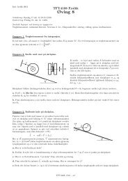
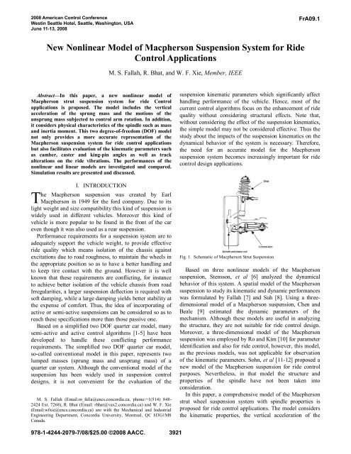
Fig. 1. Schematic <strong>of</strong> <strong>Macpherson</strong> Strut <strong>Suspension</strong><br />
FrA09.1<br />
Based on three nonlinear models <strong>of</strong> the <strong>Macpherson</strong><br />
suspension, Stensson, et al [6] analyzed the dynamical<br />
behavior <strong>of</strong> this system. A spatial model <strong>of</strong> the <strong>Macpherson</strong><br />
suspension to study its kinematic and dynamic per<strong>for</strong>mances<br />
was <strong>for</strong>mulated by Fallah [7] and Suh [8]. Using a threedimensional<br />
model <strong>of</strong> a <strong>Macpherson</strong> suspension, Chen and<br />
Beale [9] estimated the dynamic parameters <strong>of</strong> the<br />
mechanism. Although these models are useful in analyzing<br />
the structure, they are not suitable <strong>for</strong> ride control design.<br />
Moreover, a three-dimensional model <strong>of</strong> the <strong>Macpherson</strong><br />
suspension was employed by Ro and Kim [10] <strong>for</strong> parameter<br />
identification and also <strong>for</strong> ride control, however, this model,<br />
as the previous models, was not applicable <strong>for</strong> observation<br />
<strong>of</strong> the kinematic parameters. Sohn, et al [11-12] proposed a<br />
new model <strong>of</strong> the <strong>Macpherson</strong> suspension <strong>for</strong> ride control<br />
purposes. Nevertheless, in that model the structure and<br />
properties <strong>of</strong> the spindle have not been taken into<br />
consideration.<br />
In this paper, a comprehensive model <strong>of</strong> the <strong>Macpherson</strong><br />
strut wheel suspension system with spindle properties is<br />
proposed <strong>for</strong> ride control applications. The model considers<br />
the kinematic properties, the vertical acceleration <strong>of</strong> the
sprung mass and the motions <strong>of</strong> the unsprung mass subjected<br />
to control arm rotation. In addition, it includes physical<br />
characteristics <strong>of</strong> the spindle such as mass and inertia<br />
moment. With this model, it is convenient to observe the<br />
suspension kinematic parameters subjected to control<br />
actuation <strong>for</strong>ce, designed to improve the ride quality.<br />
II. NEW MODEL OF MACPHERSON SUSPENSION FOR ACTIVE<br />
CONTROL APPLICATIONS<br />
The schematic <strong>of</strong> a <strong>Macpherson</strong> strut suspension is shown in<br />
Fig.1. To model a <strong>Macpherson</strong> suspension system <strong>for</strong><br />
control application, one should take into account both the<br />
kinematics and dynamics <strong>of</strong> the system subjected to the<br />
actuation <strong>for</strong>ce and road disturbances.<br />
A. Kinematics<br />
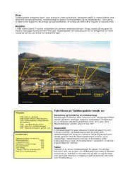
Consider a <strong>Macpherson</strong> suspension system excited by road<br />
disturbance (zr) as shown in Fig. 2. It comprises a quarter-car<br />
body, a spindle and a tire, a helical spring, control arm, load<br />
disturbance (fd) and an actuation <strong>for</strong>ce (fa). The structure has<br />
two degrees <strong>of</strong> freedom including vertical displacement <strong>of</strong><br />
the sprung mass and rotational motion <strong>of</strong> the control arm<br />
when the mass <strong>of</strong> the strut is ignored and the bushing at<br />
point D is assumed to be a pin joint. In this research, we<br />
focus on building a two DOF model <strong>of</strong> a <strong>Macpherson</strong><br />
suspension system.<br />
Fig. 2. <strong>Model</strong> <strong>of</strong> <strong>Macpherson</strong> suspension<br />
The detailed assumptions in this modeling are made as<br />
follows: The sprung mass has only vertical displacement<br />
while movements in other directions are ignored. The<br />
unsprung mass (spindle and tire) is connected to the car<br />
body through the damper and spring as well as the control<br />
arm. The values <strong>of</strong> zs, vertical displacement <strong>of</strong> the sprung<br />
mass, and θ, rotational displacement <strong>of</strong> the control arm, are<br />
measured from the static equilibrium position and are<br />
considered as generalized coordinates. It is assumed that, in<br />
the equilibrium condition, the camber angle is zero.<br />
Compared to the other links, the mass and stiffness <strong>of</strong> the<br />
strut are neglected. The spring and tire deflections and the<br />
damping <strong>for</strong>ce are assumed to be in the linear regions <strong>of</strong><br />
their operation ranges.<br />
In Fig. 2, link AB represents the control arm which is<br />
modeled as a rod, while line CD shows the strut <strong>of</strong> the<br />
mechanism. The revolute joint, located between the control<br />
arm and the chassis, is modeled as a rotational joint at point<br />
B. In addition, let assume that the origin <strong>of</strong> the coordinate<br />
system, O, is on point B and (yA, zA), (yB, zB), (yJ, zJ), (yp,<br />
zp), (yC, zC) and (yD, zD) denote the coordinates <strong>of</strong> the points<br />
A, B, J, P, C and D, respectively. Under road disturbances,<br />
the position <strong>of</strong> the key points on the sprung mass change as<br />
the following:<br />
y =<br />
+<br />
B<br />
, zB<br />
= zs<br />
, = zD<br />
= zD<br />
zs<br />
, y y<br />
0 D D<br />
(1)<br />
1<br />
In addition, the displacements <strong>of</strong> the main points on the<br />
spindle are introduced as:<br />
⎡yC<br />
⎢<br />
⎢<br />
zC<br />
⎢⎣<br />
1<br />
yJ<br />
z J<br />
1<br />
yP<br />
⎤ ⎡a11<br />
z<br />
⎥<br />
=<br />
⎢<br />
P ⎥ ⎢<br />
a21<br />
1 ⎥⎦<br />
⎢⎣<br />
0<br />
⎡y<br />
C y ⎤<br />
1 J y<br />
1 P1<br />
⎢ ⎥<br />
⎢<br />
zC<br />
z<br />
1 J z<br />
1 P1<br />
⎥<br />
⎢⎣<br />
1 1 1 ⎥⎦<br />
a<br />
a<br />
12<br />
22<br />
0<br />
yA<br />
− ( a11y<br />
A + a<br />
1 12z<br />
z A − ( a21y<br />
A + a<br />
1 22z<br />
1<br />
1<br />
A<br />
1<br />
A<br />
1<br />
) ⎤<br />
)<br />
⎥<br />
⎥<br />
×<br />
⎥⎦<br />
where (yA1, zA1), (yJ1, zJ1) , (yP1, zP1), (yC1, zC1) are the<br />
coordinates <strong>of</strong> the points A, J, P and C at equilibrium<br />
position. Further,<br />
a<br />
a<br />
3922<br />
11<br />
12<br />
= a22<br />
= cosϕ<br />
= −a<br />
= sinϕ<br />
21<br />
where φ is the rotation angle <strong>of</strong> the wheel. <strong>System</strong> <strong>of</strong><br />
equations (2), is made <strong>of</strong> six equations containing nine<br />
unknown parameters which are (yA, zA), (yJ, zJ), (yP, zP), (yC,<br />
zC) and φ.<br />
To solve this system, it is necessary to employ constraint<br />
equations as follows:<br />
z C =α( yC − y D ) + zD<br />
z J =α( yJ − y D ) + zD<br />
y = L cos( θ+θ ) + y<br />
z = L sin( θ+θ ) + z<br />
A A 1 B<br />
A A 1 B<br />
where α is the slope <strong>of</strong> the strut, LA is the length <strong>of</strong> the<br />
control arm and θ1 is the initial angle <strong>of</strong> the control arm<br />
resulting from the static deflection and structure design.<br />
Considering equations (2) and (4), results in ten equations<br />
including ten unknown parameters, namely, (yA, zA), (yJ, zJ),<br />
(yP, zP), (yC, zC), α and φ. Thus, the following equations <strong>of</strong><br />
displacements can be established:<br />
(2)<br />
(3)<br />
(4)
y<br />
z<br />
y<br />
z<br />
y<br />
z<br />
z<br />
z<br />
y<br />
z<br />
C<br />
C<br />
J<br />
J<br />
P<br />
P<br />
C<br />
J<br />
A<br />
A<br />
= ( y<br />
= ( y<br />
= ( y<br />
C1<br />
C1<br />
J1<br />
= ( y<br />
J<br />
= ( y<br />
= ( y<br />
P<br />
P<br />
= α(<br />
y<br />
= α(<br />
y<br />
= L<br />
= L<br />
A<br />
A<br />
− y<br />
− y<br />
− y<br />
1<br />
1<br />
1<br />
C<br />
J<br />
A1<br />
A1<br />
A1<br />
− y<br />
− y<br />
− y<br />
) a<br />
) a<br />
) a<br />
A<br />
A<br />
A<br />
1<br />
1<br />
1<br />
− y<br />
− y<br />
D<br />
D<br />
11<br />
21<br />
11<br />
) a<br />
) a<br />
) a<br />
+ ( z<br />
+ ( z<br />
+ ( z<br />
21<br />
11<br />
21<br />
) + z<br />
) + z<br />
cos( θ + θ )<br />
A1<br />
C1<br />
A1<br />
+ ( z<br />
+ ( z<br />
+ ( z<br />
D<br />
D<br />
sin( θ + θ ) + z<br />
1<br />
1<br />
s<br />
− z<br />
− z<br />
C1<br />
A1<br />
J1<br />
) a<br />
) a<br />
21<br />
11<br />
+ y<br />
+ z<br />
A<br />
− z ) a + y<br />
J<br />
A<br />
P<br />
1<br />
1<br />
1<br />
− z<br />
− z<br />
− z<br />
A<br />
P<br />
A<br />
21<br />
1<br />
1<br />
1<br />
) a<br />
) a<br />
) a<br />
11<br />
21<br />
11<br />
A<br />
A<br />
+ z<br />
+ y<br />
+ z<br />
When solving the above system <strong>of</strong> equations, one determines<br />
parameter φ as a function <strong>of</strong> generalized coordinates θ and<br />
zs. Subsequently, the other unknown parameters including<br />
(yA, zA), (yJ, zJ), (yP, zP), (yC, zC) and α can be specified.<br />
Hence, the displacements <strong>of</strong> all key points are determined as<br />
functions <strong>of</strong> independent variables θ and zs. The next step is<br />
to find the velocities <strong>of</strong> the key points. By taking the<br />
derivative <strong>of</strong> (5), one can obtain the velocity components <strong>of</strong><br />
the main points. When solving the equations <strong>of</strong> velocities,<br />
the value <strong>of</strong> ϕ� is determined as following:<br />
( z�<br />
A − ay�<br />
A − z�<br />
D )( yC<br />
− yJ<br />
)<br />
ϕ�<br />
=<br />
(6)<br />
h<br />
where<br />
h = ( yC<br />
− yA<br />
+ αzC<br />
− αz<br />
A )( yJ<br />
− y<br />
( y − y + αz<br />
− αz<br />
)( y − y )<br />
J<br />
A<br />
J<br />
A<br />
C<br />
D<br />
D<br />
) −<br />
B. Equations <strong>of</strong> Motion<br />
Lagrange’s method is used to obtain the equations <strong>of</strong> motion<br />
<strong>of</strong> the new model. The kinetic energy, T, is given by<br />
1<br />
2 1 2 2 1 2 1 B 2<br />
T = ( m + � + � + � + ϕ�<br />
+ θ�<br />
s mca<br />
)( zs<br />
) mu(<br />
yP<br />
zP<br />
) Iu<br />
Ica<br />
2<br />
2<br />
2 2<br />
(7)<br />
where ms, mu and mca, are the car body, wheel and control<br />
arm masses, respectively. Iu and B<br />
I ca represent, in turn, the<br />
inertia moments <strong>of</strong> the wheel and the control arm where the<br />
latter is around point B. The potential energy, V, is defined<br />
as<br />
1 2 1 2<br />
V = Ks<br />
( ∆ L)<br />
+ Kt<br />
( ∆z)<br />
(8)<br />
2 2<br />
where Ks and Kt are the stiffness coefficients <strong>of</strong> the sprung<br />
and unsprung masses, respectively. Moreover, the deflection<br />
<strong>of</strong> the spring ∆ L , and the deflection <strong>of</strong> the tire ∆z are:<br />
2<br />
2 ( 1/<br />
2 )<br />
∆ L = [( y − y ) + ( z − z ) ] −<br />
C<br />
D<br />
C<br />
D<br />
A<br />
A<br />
A<br />
(5)<br />
[( y<br />
C 1<br />
D<br />
1<br />
2<br />
C1<br />
D<br />
1<br />
( 1 / 2 )<br />
− y ) + ( z − z )]<br />
(9)<br />
∆ z = z − z = ( y − y ) ϕ + ( z − z ) +<br />
A<br />
P<br />
r<br />
A1<br />
s<br />
P1<br />
L sin( θ + θ1<br />
) + z − z<br />
(10)<br />
r<br />
P1<br />
The damping function, D, is given by<br />
1 2<br />
= C ( ∆L�<br />
)<br />
(11)<br />
2<br />
D p<br />
where Cp is the damping coefficient and the relative velocity<br />
<strong>of</strong> damper L� ∆ is:<br />
A1<br />
∆ � = [ y�<br />
( y − y ) + ( z�<br />
− z�<br />
)( z − z )] ×<br />
[(<br />
3923<br />
L C C D C D C D<br />
yC<br />
2 2 ( −1/<br />
2 )<br />
yD<br />
) + ( zC<br />
− zD<br />
) ]<br />
− (12)<br />
substituting the values <strong>of</strong> y� p and z� p , obtained from<br />
derivative <strong>of</strong> (5), and ϕ� , attained from (6), into (7) as well<br />
as using Lagrange’s equations along with the generalized<br />
coordinates zs and θ, one can obtain the accelerations <strong>of</strong> the<br />
generalized coordinates as the following:<br />
[<br />
( ms<br />
+ mu<br />
+ mca<br />
) �z<br />
�s<br />
+ mu<br />
LA<br />
cos( θ + θ1)<br />
+ cos( θ + θ1)<br />
+<br />
( yC<br />
− yJ<br />
)( yP<br />
− y A)<br />
⎤<br />
α sin( θ θ ] � θ�<br />
��<br />
� θ�<br />
(13)<br />
+ 1)<br />
= f1z<br />
s + f 2<br />
h<br />
⎥<br />
⎦<br />
and<br />
⎡<br />
∂ � ϕ ⎤<br />
mu ⎢L<br />
A cos( θ + θ1<br />
) + ( yP<br />
− z A)<br />
⎥<br />
�z<br />
�s<br />
+<br />
⎣<br />
∂ � θ ⎦<br />
⎡ ⎡<br />
( yC<br />
− yJ<br />
)( z<br />
⎢ ⎢{<br />
(cos( θ + θ1)<br />
+ α sin( θ + θ1)<br />
}<br />
m<br />
⎢ u LA<br />
h<br />
⎢<br />
⎢⎣<br />
⎢⎣<br />
− sin( θ + θ1)<br />
⎡<br />
∂ � ϕ ⎤<br />
⎢−<br />
L A sin( θ + θ1)<br />
+ ( z A − z P ) ⎥ +<br />
⎣<br />
∂ � θ ⎦<br />
⎡<br />
∂ � ϕ ⎤<br />
mu<br />
LA<br />
⎢L<br />
A cos( θ + θ1)<br />
+ ( yP<br />
− z A)<br />
⎥ ×<br />
⎣<br />
∂ � θ ⎦<br />
⎡<br />
( yC<br />
− yJ<br />
)( y<br />
⎢{<br />
(cos( θ + θ1)<br />
+ α sin( θ + θ1)<br />
}<br />
h<br />
⎢<br />
⎢⎣<br />
+ cos( θ + θ1)<br />
∂ � ϕ<br />
� ϕ�<br />
⎤<br />
I � θ�<br />
��<br />
� θ�<br />
u = f<br />
� 3zs<br />
+ f4<br />
∂θ<br />
⎥<br />
⎦<br />
[<br />
P<br />
− y<br />
A<br />
A<br />
− z<br />
) ⎤<br />
⎥ +<br />
⎥<br />
⎥⎦<br />
P<br />
) ⎤<br />
⎥ ×<br />
⎥<br />
⎥⎦<br />
(14)<br />
Since the equations are highly nonlinear and too<br />
complicated, the higher order nonlinearities in Eqs. 13 and<br />
14 are ignored to simplify the equations. Let us denote
H<br />
∂T<br />
,<br />
∂V<br />
,<br />
1 = − H 2 =<br />
H3<br />
∂zs<br />
∂zs<br />
= −<br />
∂D<br />
∂z�<br />
∂T<br />
∂V<br />
∂D<br />
H4 = − , H5<br />
= , H6<br />
= −<br />
∂θ<br />
∂θ<br />
∂ � θ<br />
Hence, one has<br />
�� � θ �<br />
�<br />
∂r<br />
C<br />
f1 zs<br />
+ f2<br />
s = . fa<br />
+ fd<br />
+ H3<br />
− H1<br />
− H 2 = F1<br />
∂zs<br />
and<br />
�<br />
∂r<br />
f3 � z�<br />
C<br />
s + f �<br />
4θ�<br />
= − . fa<br />
+ H6<br />
− H 4 − H5<br />
= F2<br />
.<br />
∂θ<br />
The nonlinear equations <strong>of</strong> motion are obtained as below<br />
f1(<br />
z , , θ , � θ ) 2 ( , , θ,<br />
� θ ) � θ�<br />
1(<br />
, , θ , �<br />
s z�<br />
s �z<br />
�s<br />
+ f z s z�<br />
s = F z s z�<br />
s θ )<br />
f3<br />
( z , � , θ,<br />
� θ ) ��<br />
4 ( , � , θ , � θ ) � θ�<br />
2 ( , � , θ , �<br />
s z s z s + f z s z s = F z s z s θ )<br />
(15)<br />
Solving the above system, the acceleration <strong>of</strong> the generalized<br />
coordinates are obtained as follows:<br />
f4F1<br />
− f2F<br />
�<br />
2<br />
z�<br />
1(<br />
, � , θ , �<br />
s =<br />
= g zs<br />
zs<br />
θ )<br />
f f − f f<br />
4<br />
4<br />
1<br />
1<br />
2<br />
2<br />
3<br />
3<br />
� 1 2 3 1<br />
θ�<br />
f F − f F<br />
=<br />
= g2(<br />
z , � , θ , �<br />
s zs<br />
θ )<br />
f f − f f<br />
s<br />
(16)<br />
At this point let us introduce the state variables as [x1, x2, x3,<br />
x4] T<br />
T<br />
[ z s , zs<br />
, θ, θ ] �<br />
= � , then (16) can be written in the state<br />
space <strong>for</strong>mat as follows.<br />
x�<br />
1 = x2<br />
x�<br />
= g ( z , z�<br />
, θ , � θ,<br />
f , f , z )<br />
2<br />
x�<br />
3<br />
x�<br />
4<br />
1<br />
2<br />
s<br />
s<br />
s<br />
= x4<br />
= g ( z , z�<br />
, θ,<br />
� θ , f , f , z )<br />
s<br />
a<br />
a<br />
d<br />
d<br />
r<br />
r<br />
(17)<br />
Since the equations are nonlinear and working with them is<br />
non-trivial task and employing a complex nonlinear<br />
controller is essential, all <strong>of</strong> equations are linearized at the<br />
equilibrium state where, (x1e, x2e, x3e, x4e) = (0, 0, 0, 0). The<br />
resulting equations are:<br />
x�<br />
= Ax<br />
x(<br />
0)<br />
= xe<br />
⎡ 0<br />
⎢∂g1<br />
⎢ ∂x<br />
A = ⎢ 1<br />
⎢ 0<br />
⎢∂g1<br />
⎢⎣<br />
∂x1<br />
( t)<br />
+ B1<br />
fa<br />
( t)<br />
+ B2z<br />
r ( t)<br />
+ B3<br />
1<br />
∂g<br />
∂x<br />
0<br />
∂g<br />
∂x<br />
1<br />
2<br />
2<br />
2<br />
0<br />
∂g<br />
∂x<br />
0<br />
∂g<br />
∂x<br />
1<br />
3<br />
2<br />
3<br />
0 ⎤<br />
∂g1<br />
⎥<br />
∂x<br />
⎥<br />
4 ⎥<br />
1 ⎥<br />
∂g2<br />
⎥<br />
∂x4<br />
⎥⎦<br />
xe<br />
f ( t)<br />
d<br />
(18)<br />
⎡<br />
B1<br />
= ⎢0<br />
⎣<br />
B<br />
B<br />
3924<br />
2<br />
3<br />
⎡<br />
= ⎢0<br />
⎣<br />
⎡<br />
= ⎢0<br />
⎣<br />
∂g<br />
∂f<br />
1<br />
a<br />
∂g<br />
∂z<br />
1<br />
r<br />
∂g<br />
∂f<br />
1<br />
d<br />
0<br />
0<br />
0<br />
∂g<br />
∂f<br />
2<br />
a<br />
⎤<br />
⎥<br />
⎦<br />
∂g2<br />
⎤<br />
⎥<br />
∂zr<br />
⎦<br />
∂g<br />
∂f<br />
2<br />
d<br />
f = 0<br />
a<br />
z = 0<br />
⎤<br />
⎥<br />
⎦<br />
r<br />
f = 0<br />
d<br />
III. SIMULATION AND VERIFICATION OF MODEL<br />
A. Comparison <strong>of</strong> the conventional, linear and nonlinear<br />
models<br />
In order to compare the models, the following values have<br />
been taken from [12] and ADAMS s<strong>of</strong>tware default:<br />
ms<br />
= 453 (Kg), mu<br />
= 71(Kg),<br />
K s = 17658 (N/m)<br />
2<br />
Kt<br />
= 183887 (N/m), Iu<br />
= 0.021 (Kg.m )<br />
C p = 1950 (N.sec/m)<br />
The positions <strong>for</strong> the key points on the <strong>Macpherson</strong><br />
suspension are considered as the below (all dimensions are<br />
in mm):<br />
A1<br />
= ( 206.5, 249, - 60.8), C1<br />
= ( 222, 152.6, 236.2)<br />
J1<br />
= ( 229.2 , 134.5, 374.8), P1<br />
= ( 211.1, 292.1, 27.5)<br />
D1<br />
= (240, 107.4, 582.5)<br />
The output variables <strong>of</strong> the conventional model are the<br />
vertical displacements <strong>of</strong> the sprung mass z s and the<br />
unsprung mass z u whereas in the new model the output<br />
vector consists <strong>of</strong> the displacement <strong>of</strong> the sprung mass z s<br />
and the angular displacement <strong>of</strong> the control arm θ. Thus, the<br />
displacement <strong>of</strong> the sprung mass, z s , is considered as the<br />
output variable in order to compare the two models . The<br />
frequency response <strong>of</strong> the two models is shown in Fig. 3. As<br />
can be seen, the first resonance frequency is smaller than<br />
that <strong>of</strong> the conventional model and the second resonant<br />
frequency is larger than that <strong>of</strong> the conventional model.<br />
In the literature, the acceleration <strong>of</strong> the sprung mass is<br />
considered as a criterion <strong>for</strong> assessment <strong>of</strong> the effect <strong>of</strong> a<br />
suspension on the ride com<strong>for</strong>t, specially, in the high<br />
frequency ranges. Fig. 4 compares the acceleration<br />
transmissibility <strong>of</strong> three models <strong>for</strong> frequencies between 0-<br />
20 Hz. As shown in Fig. 4, the linear model represents a<br />
good per<strong>for</strong>mance <strong>of</strong> the nonlinear model <strong>for</strong> the frequencies<br />
between 0-5 Hz. However, the conventional model shows<br />
the per<strong>for</strong>mance <strong>of</strong> the <strong>Macpherson</strong> suspension systems with<br />
some discrepancies.
Fig. 3 Frequency response <strong>of</strong> new model and conventional model<br />
Fig. 4 Acceleration transmissibility <strong>of</strong> the nonlinear, linear and conventional<br />
models<br />
B. Evaluation <strong>of</strong> the kinematic parameters<br />
Some <strong>of</strong> the main kinematical parameters which are<br />
important in chassis design and affect handling and stability<br />
<strong>of</strong> the vehicle are 1) camber angle; 2) kingpin angle 3) caster<br />
angle 4) track. Camber angle alterations are due to rubbing<br />
<strong>of</strong> tires and produce lateral <strong>for</strong>ces acting on the wheel and<br />
cause the vehicle to steer to one side. Alterations <strong>of</strong> kingpin<br />
and caster angles affect the self aligning torques and<br />
consequently affect the stability and handling <strong>of</strong> the vehicle<br />
when wheels bounce or rebound. When the wheels travel on<br />
a bump and rebound, the track changes cause the rolling tire<br />
to slip and, also produce lateral <strong>for</strong>ces [13]. In the following<br />
simulations, we set the step input <strong>for</strong> road disturbance zr<br />
equal to 100 mm and time step equal to 0.0001 (s).<br />
The camber angle, represented by φ in (3), is the angle<br />
between the wheel center plane and a vertical line to the road<br />
[13]. Fig. 5 shows this parameter variation <strong>for</strong> both the linear<br />
and the nonlinear models. In definition, the steering axis is<br />
the line passing through the point D and A in the threedimensional<br />
case and the kingpin angle is the angle between<br />
the projection <strong>of</strong> the steering axis on y-z plane and the<br />
vertical line to the road. In Fig. 6, King-Pin angle variations<br />
are plotted <strong>for</strong> both the linear and nonlinear models. The<br />
angle between the projection <strong>of</strong> the steering axis on the x-z<br />
3925<br />
plane and the vertical line to the road is defined as caster<br />
angle. The per<strong>for</strong>mance <strong>of</strong> this parameter is illustrated in<br />
Fig. 7. Track is the lateral distance between the centers <strong>of</strong><br />
the front wheels. Fig. 8 shows the alteration <strong>of</strong> track <strong>for</strong> the<br />
linear and nonlinear models. It is obvious that, unlike the<br />
previous parameters, the linearization has a large impact on<br />
the track. As a result, linear model is not sufficiently<br />
accurate <strong>for</strong> studying the track behavior.<br />
Fig. 5 Camber angle alterations<br />
Fig. 6 King-pin angle alterations<br />
Fig. 7 Caster angle alterations
Fig. 7 Track alteration<br />
IV. CONCLUSION<br />
A new nonlinear model <strong>of</strong> <strong>Macpherson</strong> suspension is<br />
proposed and equations <strong>of</strong> motion are derived. The new<br />
model is more general than conventional model where the<br />
structural kinematics and spindle properties are taken into<br />
account. In addition, the new model allows investigation <strong>of</strong><br />
the suspension kinematic parameters affecting on handling<br />
and stability <strong>of</strong> the vehicle while it is impossible or difficult<br />
using the other models proposed <strong>for</strong> the <strong>Macpherson</strong><br />
suspension in the case <strong>of</strong> ride control implementation. The<br />
nonlinear and linear responses <strong>of</strong> the model are investigated<br />
and shown that the linear model is a good approximation <strong>of</strong><br />
the nonlinear model <strong>for</strong> ride quality assessment. However,<br />
<strong>for</strong> evaluation <strong>of</strong> the kinematic parameter per<strong>for</strong>mances<br />
nonlinear kinematic relations are used which provide a more<br />
accurate study <strong>of</strong> handling per<strong>for</strong>mance and stability<br />
condition <strong>of</strong> the vehicle.<br />
REFERENCES<br />
[1] M. Ahmadian, N. Vahdati, “Transient response <strong>of</strong> semi-active<br />
suspensions with hybrid control”, J. <strong>of</strong> Intelligent Materials <strong>System</strong>s<br />
and Structures, vol. 17, pp. 145-153, 2006..<br />
[2] M. Ahmadian, C. Pare, “A quarter-car experimental analysis <strong>of</strong><br />
alternative semiactive control methods”, J. <strong>of</strong> Intelligent Materials<br />
<strong>System</strong>s and Structures, vol. 11, pp. 604-612, 2000.<br />
[3] Y. Zhang, A. Alleyne, “A practical and effective approach to active<br />
suspension control”, J. <strong>of</strong> Vehicle <strong>System</strong> Dynamics, vol. 43, no. 5, pp.<br />
305-330, 2005.<br />
[4] W. Sie, R. Lian, B., Lin, “Enhancing grey prediction fuzzy controller<br />
<strong>for</strong> active suspension systems”, J. <strong>of</strong> Vehicle <strong>System</strong> Dynamics, vol.<br />
44, no. 5, pp. 407-430, 2006.<br />
[5] J. Lin, I. Kanellakopoulos, “<strong>Nonlinear</strong> design <strong>of</strong> active suspension”,<br />
IEEE Control <strong>System</strong> Magazine, vol. 17, pp. 45-49, 1995.<br />
[6] A. Stensson, C. Splund, Karlsson, “The nonlinear behavior <strong>of</strong> a<br />
<strong>Macpherson</strong> suspension mechanism”, J. <strong>of</strong> Vehicle <strong>System</strong> Dynamics,<br />
vol. 39, no. 3, pp. 85-106, 1994.<br />
[7] M. S. Fallah, “Kinematical and dynamical analysis <strong>of</strong> <strong>Macpherson</strong><br />
suspension”, M. Sc. Thesis, Mech. Eng. Dept., Shiraz University,<br />
Shiraz, Iran, 2004 (in Persian).<br />
3926<br />
[8] C. H. Suh, “Synthesis and analysis <strong>of</strong> suspension mechanism with use<br />
<strong>of</strong> displacement matrices”, SAE Technical Paper Series, Paper No.<br />
890098, 1989.<br />
[9] K. Chen, D. G. Beale, “Base dynamic parameter estimation <strong>of</strong> a<br />
<strong>Macpherson</strong> suspension mechanism”, J. <strong>of</strong> Vehicle <strong>System</strong> Dynamics,<br />
vol. 39, no. 3, pp. 227-244, 2003.<br />
[10] C. Kim, P. I. Ro, “Reduced Order <strong>Model</strong>ing and Parameter Estimation<br />
<strong>for</strong> Quarter Car <strong>Suspension</strong> <strong>System</strong>” J. <strong>of</strong> Automobile Engineering,<br />
IMechE, vol. 214, part D, pp. 851-864, 2000.<br />
[11] K. S. Hong, D. S. Jeon, H. C. Sohn, “A new modeling <strong>of</strong> the<br />
<strong>Macpherson</strong> suspension system and its optimal pole-placement<br />
control”, Proceedings <strong>of</strong> the 7th Mediterranean Conference on Control<br />
and Automation (MED99) Haifa, Israel, June 28-30, 1999.<br />
[12] H. C. Sohn, K. S. Hong, J. K. Hedrick, “Modified skyhook control <strong>of</strong><br />
semi-active suspensions: a new model, gain scheduling, and hardwarein-the-Loop<br />
tuning”, J. <strong>of</strong> Dynamic <strong>System</strong>s, Measurement, and<br />
Control, vol. 124, no. 1, pp. 158-167, 2002.<br />
[13] J. Reimpell, H. Stoll, J. W. Betzler, The automotive chassis:<br />
engineering principles, 2 ed edition, Butterworth Heinmann, 2001.