Lines, Curves and Surfaces in 3D
Lines, Curves and Surfaces in 3D
Lines, Curves and Surfaces in 3D

You also want an ePaper? Increase the reach of your titles
YUMPU automatically turns print PDFs into web optimized ePapers that Google loves.
<strong>L<strong>in</strong>es</strong>, <strong>Curves</strong> <strong>and</strong> <strong>Surfaces</strong> <strong>in</strong> <strong>3D</strong><br />
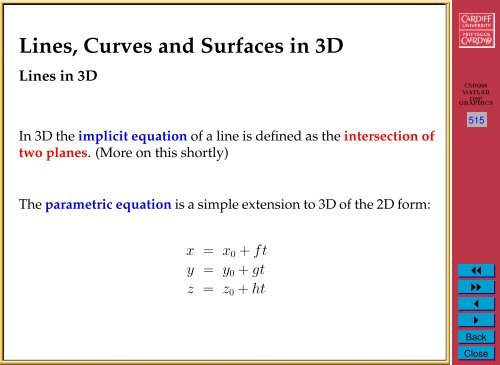
<strong>L<strong>in</strong>es</strong> <strong>in</strong> <strong>3D</strong><br />
In <strong>3D</strong> the implicit equation of a l<strong>in</strong>e is def<strong>in</strong>ed as the <strong>in</strong>tersection of<br />
two planes. (More on this shortly)<br />
CM0268<br />
MATLAB<br />
DSP<br />
GRAPHICS<br />
515<br />
The parametric equation is a simple extension to <strong>3D</strong> of the 2D form:<br />
x = x 0 + ft<br />
y = y 0 + gt<br />
z = z 0 + ht<br />
1<br />
◭◭<br />
◮◮<br />
◭<br />
◮<br />
Back<br />
Close
Parametric <strong>L<strong>in</strong>es</strong> <strong>in</strong> <strong>3D</strong><br />
w<br />
p =(x, y, z)<br />
v 0 =(x 0 ,y 0 ,z 0 )<br />
v<br />
tw<br />
v + tw<br />
CM0268<br />
MATLAB<br />
DSP<br />
GRAPHICS<br />
516<br />
x = x 0 + ft<br />
y = y 0 + gt<br />
z = z 0 + ht<br />
1<br />
This is simply an extension of the vector form <strong>in</strong> <strong>3D</strong><br />
The l<strong>in</strong>e is normalised when f 2 + g 2 + h 2 = 1<br />
◭◭<br />
◮◮<br />
◭<br />
◮<br />
Back<br />
Close
Perpendicular Distance from a Po<strong>in</strong>t to a L<strong>in</strong>e <strong>in</strong> <strong>3D</strong><br />
For the parametric form,<br />
x = x 0 + ft<br />
y = y 0 + gt<br />
z = z 0 + ht<br />
CM0268<br />
MATLAB<br />
DSP<br />
GRAPHICS<br />
517<br />
This builds on the 2D example we met earlier, l<strong>in</strong>e par po<strong>in</strong>t dist 2d.<br />
The <strong>3D</strong> form is l<strong>in</strong>e par po<strong>in</strong>t dist 3d.<br />
dx = g * ( f * ( p(2) - y0 ) - g * ( p(1) - x0 ) ) ...<br />
+ h * ( f * ( p(3) - z0 ) - h * ( p(1) - x0 ) );<br />
dy = h * ( g * ( p(3) - z0 ) - h * ( p(2) - y0 ) ) ...<br />
- f * ( f * ( p(2) - y0 ) - g * ( p(1) - x0 ) );<br />
1<br />
dz = - f * ( f * ( p(3) - z0 ) - h * ( p(1) - x0 ) ) ...<br />
- g * ( g * ( p(3) - z0 ) - h * ( p(2) - y0 ) );<br />
dist = sqrt ( dx * dx + dy * dy + dz * dz ) ...<br />
/ ( f * f + g * g + h * h );<br />
The value of parameter, t, where the po<strong>in</strong>t <strong>in</strong>tersects the l<strong>in</strong>e is<br />
given by:<br />
t =<br />
(f*( p(1) - x0) + g*(p(2) - y0) + h*(p(3) - z0)/( f * f + g * g + h*h);<br />
◭◭<br />
◮◮<br />
◭<br />
◮<br />
Back<br />
Close
L<strong>in</strong>e Through Two Po<strong>in</strong>ts <strong>in</strong> <strong>3D</strong> (parametric form)<br />
Q<br />
P<br />
The parametric form of a l<strong>in</strong>e through two po<strong>in</strong>ts, P (x p , y p , z p ) <strong>and</strong><br />
Q(x q , y q , z q ) comes readily from the vector form of l<strong>in</strong>e (aga<strong>in</strong> a simple<br />
extension from 2D):<br />
• Set base to po<strong>in</strong>t P<br />
• Vector along l<strong>in</strong>e is (x q − x p , y q − y p , z q − z p )<br />
• The equation of the l<strong>in</strong>e is:<br />
x = x p + (x q − x p )t<br />
y = y p + (y q − y p )t<br />
z = z p + (z q − z p )t<br />
• As <strong>in</strong> 2D, t = 0 gives P <strong>and</strong> t = 1 gives Q<br />
• Normalise if necessary.<br />
CM0268<br />
MATLAB<br />
DSP<br />
GRAPHICS<br />
518<br />
1<br />
◭◭<br />
◮◮<br />
◭<br />
◮<br />
Back<br />
Close
Implicit <strong>Surfaces</strong><br />
An implicit surface (just like implicit curves <strong>in</strong> 2D) of the form<br />
f(x, y, z) = 0<br />
We simply add the extra z dimension.<br />
For example:<br />
CM0268<br />
MATLAB<br />
DSP<br />
GRAPHICS<br />
519<br />
• A plane can be represented<br />
ax + by + cz + d = 0<br />
• A sphere can be represented as<br />
(x − x c ) 2 + (y − y c ) 2 + (z − z c ) 2 − r 2 = 0<br />
which is just the extension of the circle <strong>in</strong> 2D to <strong>3D</strong> where the<br />
centre is now (x c , y c , z c ) <strong>and</strong> the radius is r.<br />
1<br />
◭◭<br />
◮◮<br />
◭<br />
◮<br />
Back<br />
Close
Implicit Equation of a Plane<br />
(a, b, c)<br />
CM0268<br />
MATLAB<br />
DSP<br />
GRAPHICS<br />
520<br />
d<br />
The plane equation:<br />
O<br />
ax + by + cz + d = 0<br />
• Is normalised if a 2 + b 2 + c 2 = 1.<br />
• Like 2D the normal vector — the surface normal — is given by a<br />
vector n = (a, b, c)<br />
– a, b <strong>and</strong> c are the cos<strong>in</strong>e angles which the normal makes with<br />
the x-,y- <strong>and</strong> z-axes respectively.<br />
1<br />
◭◭<br />
◮◮<br />
◭<br />
◮<br />
Back<br />
Close
Parametric Equation of a Plane<br />
(x 0 ,y 0 ,z 0 )<br />
(f 1 ,g 1 ,h 1 )<br />
(f 2 ,g 2 ,h 2 )<br />
CM0268<br />
MATLAB<br />
DSP<br />
GRAPHICS<br />
521<br />
O<br />
x = x 0 + f 1 u + f 2 v<br />
y = y 0 + g 1 u + g 2 v<br />
z = z 0 + h 1 u + h 2 v<br />
1<br />
• This is an extension of parametric l<strong>in</strong>e <strong>in</strong>to <strong>3D</strong> where we now<br />
have two variable parameters u <strong>and</strong> v that vary.<br />
• (f 1 , g 1 , h 1 ) <strong>and</strong> (f 2 , g 2 , h 2 ) are two different vectors parallel to the<br />
plane.<br />
◭◭<br />
◮◮<br />
◭<br />
◮<br />
Back<br />
Close
Parametric Equation of a Plane (Cont.)<br />
(x 0 ,y 0 ,z 0 )<br />
O<br />
(f 2 ,g 2 ,h 2 )<br />
(f 1 ,g 1 ,h 1 )<br />
CM0268<br />
MATLAB<br />
DSP<br />
GRAPHICS<br />
522<br />
x = x 0 + f 1 u + f 2 v<br />
y = y 0 + g 1 u + g 2 v<br />
z = z 0 + h 1 u + h 2 v<br />
• A po<strong>in</strong>t <strong>in</strong> the plane is found by add<strong>in</strong>g proportion u of one<br />
vector to a proportion v of the other vector<br />
• If the two vectors are have unit length <strong>and</strong> are perpendicular,<br />
then:<br />
f 2 1 + g 2 1 + h 2 1 = 1<br />
f 2 2 + g 2 2 + h 2 2 = 1<br />
f 1 f 2 + g 1 g 2 + h 1 h 2 = 0 (scalar product)<br />
1<br />
◭◭<br />
◮◮<br />
◭<br />
◮<br />
Back<br />
Close
Distance from a <strong>3D</strong> po<strong>in</strong>t <strong>and</strong> a Plane<br />
J(x j ,y j ,z j )<br />
d<br />
CM0268<br />
MATLAB<br />
DSP<br />
GRAPHICS<br />
523<br />
The distance, d, between a po<strong>in</strong>t, J(x j , y j , z j ), <strong>and</strong> an implicit plane,<br />
ax + by + cz + d = 0 is:<br />
d = ax j + by j + cz j + d<br />
√<br />
a2 + b 2 + c 2<br />
This is very similar the 2D distance of a po<strong>in</strong>t to a l<strong>in</strong>e.<br />
The MATALB code to achive this is, plane imp po<strong>in</strong>t dist 3d.m:<br />
norm = sqrt ( a * a + b * b + c * c );<br />
if ( norm == 0.0<br />
error ( ’PLANE Normal = 0!’ );<br />
end<br />
dist = abs ( a * p(1) + b * p(2) + c * p(3) + d ) / norm;<br />
1<br />
◭◭<br />
◮◮<br />
◭<br />
◮<br />
Back<br />
Close
Angle Between a L<strong>in</strong>e <strong>and</strong> a Plane<br />
θ<br />
CM0268<br />
MATLAB<br />
DSP<br />
GRAPHICS<br />
524<br />
If the plane is <strong>in</strong> implicit form ax + by + cz + d = 0 <strong>and</strong> l<strong>in</strong>e is <strong>in</strong><br />
parametric form:<br />
x = x 0 + ft<br />
y = y 0 + gt<br />
z = z 0 + ht<br />
then the angle, γ between the l<strong>in</strong>e <strong>and</strong> the normal the plane (a, b, c)<br />
is:<br />
γ = cos −1 (af + bg + ch)<br />
The angle, θ, between the l<strong>in</strong>e <strong>and</strong> the plane is then:<br />
θ = π 2 − γ<br />
1<br />
◭◭<br />
◮◮<br />
◭<br />
◮<br />
Back<br />
Close
Angle Between a L<strong>in</strong>e <strong>and</strong> a Plane (cont)<br />
If either l<strong>in</strong>e or plane equations are not normalised the we must<br />
normalise:<br />
γ = cos −1<br />
(af + bg + ch)<br />
√<br />
(a 2 + b 2 + c 2 ) , γ = cos−1<br />
The angle, θ, is as before:<br />
(af + bg + ch)<br />
√<br />
(f 2 + g 2 + h 2 ) , γ = cos−1<br />
(af + bg + ch)<br />
√<br />
(a 2 + b 2 + c 2 )(f 2 + g 2 + h 2 )<br />
CM0268<br />
MATLAB<br />
DSP<br />
GRAPHICS<br />
525<br />
θ = π 2 − γ<br />
The MATLAB code to so this is planes imp angle l<strong>in</strong>e 3d.m:<br />
norm1 = sqrt ( a1 * a1 + b1 * b1 + c1 * c1 );<br />
if ( norm1 == 0.0 )<br />
angle = Inf;<br />
return<br />
end<br />
norm2 = sqrt ( f * f + g *g + h * h );<br />
if ( norm2 == 0.0 )<br />
angle = Inf;<br />
return<br />
end<br />
cos<strong>in</strong>e = ( a1 * f + b1 * g + c1 * h) / ( norm1 * norm2 );<br />
angle = pi/2 - acos( cos<strong>in</strong>e );<br />
1<br />
◭◭<br />
◮◮<br />
◭<br />
◮<br />
Back<br />
Close
Angle Between Two Planes<br />
θ<br />
CM0268<br />
MATLAB<br />
DSP<br />
GRAPHICS<br />
526<br />
Given two normalised implicit planes<br />
a 1 x + b 1 y + c 1 z + d 1 = 0<br />
<strong>and</strong><br />
1<br />
a 2 x + b 2 y + c 2 z + d 2 = 0<br />
The angle between them, θ, is the angle between the normals:<br />
θ = cos −1 (a 1 a 2 + b 1 b 2 + c 1 c 2 )<br />
◭◭<br />
◮◮<br />
◭<br />
◮<br />
Back<br />
Close
Angle Between Two Planes (MATLAB Code)<br />
The MATLAB code to do this is planes imp angle 3d.m:<br />
CM0268<br />
MATLAB<br />
DSP<br />
GRAPHICS<br />
527<br />
norm1 = sqrt ( a1 * a1 + b1 * b1 + c1 * c1 );<br />
if ( norm1 == 0.0 )<br />
angle = Inf;<br />
return<br />
end<br />
1<br />
norm2 = sqrt ( a2 * a2 + b2 * b2 + c2 * c2 );<br />
if ( norm2 == 0.0 )<br />
angle = Inf;<br />
return<br />
end<br />
cos<strong>in</strong>e = ( a1 * a2 + b1 * b2 + c1 * c2 ) / ( norm1 * norm2 );<br />
angle = acos ( cos<strong>in</strong>e );<br />
◭◭<br />
◮◮<br />
◭<br />
◮<br />
Back<br />
Close
Intersection of a L<strong>in</strong>e <strong>and</strong> Plane<br />
P (x, y)<br />
CM0268<br />
MATLAB<br />
DSP<br />
GRAPHICS<br />
528<br />
If the plane is <strong>in</strong> implicit form ax + by + cz + d = 0 <strong>and</strong> l<strong>in</strong>e is <strong>in</strong><br />
parametric form:<br />
x = x 0 + ft<br />
y = y 0 + gt<br />
z = z 0 + ht<br />
The the po<strong>in</strong>t, P (x, y), where the is given by parameter, t:<br />
t = −(ax 0 + by 0 + cz 0 + d)<br />
af + bg + ch<br />
1<br />
◭◭<br />
◮◮<br />
◭<br />
◮<br />
Back<br />
Close
Intersection of a L<strong>in</strong>e <strong>and</strong> Plane (MATLAB Code)<br />
The MATLAB code to do this is plane imp l<strong>in</strong>e par <strong>in</strong>t 3d.m<br />
tol = eps;<br />
norm1 = sqrt ( a * a + b * b + c * c );<br />
if ( norm1 == 0.0 )<br />
error ( ’Norm1 = 0 - Fatal error!’ )<br />
end<br />
norm2 = sqrt ( f * f + g * g + h * h );<br />
if ( norm2 == 0.0 )<br />
error ( ’Norm2 = 0 - Fatal error!’ )<br />
end<br />
CM0268<br />
MATLAB<br />
DSP<br />
GRAPHICS<br />
529<br />
denom = a * f + b * g + c * h;<br />
if ( abs ( denom ) < tol * norm1 * norm2 ) % The l<strong>in</strong>e <strong>and</strong> the plane may be parallel.<br />
if ( a * x0 + b * y0 + c * z0 + d == 0.0 )<br />
<strong>in</strong>tersect = 1;<br />
p(1) = x0;<br />
p(2) = y0;<br />
p(3) = z0;<br />
else<br />
<strong>in</strong>tersect = 0;<br />
p(1:dim_num) = 0.0;<br />
end<br />
else<br />
<strong>in</strong>tersect = 1;<br />
t = - ( a * x0 + b * y0 + c * z0 + d ) / denom; % they must <strong>in</strong>tersect.<br />
p(1) = x0 + t * f;<br />
p(2) = y0 + t * g;<br />
p(3) = z0 + t * h;<br />
end<br />
1<br />
◭◭<br />
◮◮<br />
◭<br />
◮<br />
Back<br />
Close
Intersection of Three Planes<br />
• Three planes <strong>in</strong>tersect at po<strong>in</strong>t.<br />
• Two planes <strong>in</strong>tersect <strong>in</strong> a l<strong>in</strong>e → two l<strong>in</strong>es <strong>in</strong>tersect at a po<strong>in</strong>t<br />
• Similar problem to solv<strong>in</strong>g <strong>in</strong> 2D for two l<strong>in</strong>e <strong>in</strong>tersect<strong>in</strong>g:<br />
– Solve three simultaneous l<strong>in</strong>ear equations:<br />
CM0268<br />
MATLAB<br />
DSP<br />
GRAPHICS<br />
530<br />
a 1 x + b 1 y + c 1 z + d 1 = 0<br />
a 2 x + b 2 y + c 2 z + d 2 = 0<br />
a 3 x + b 3 y + c 3 z + d 3 = 0<br />
1<br />
◭◭<br />
◮◮<br />
◭<br />
◮<br />
Back<br />
Close
Intersection of Three Planes (MATLAB Code)<br />
The MATLAB code to do this is, planes 3d 3 <strong>in</strong>tersect.m:<br />
tol = eps;<br />
bc = b2*c3 - b3*c2;<br />
ac = a2*c3 - a3*c2;<br />
ab = a2*b3 - a3*b2;<br />
CM0268<br />
MATLAB<br />
DSP<br />
GRAPHICS<br />
531<br />
det = a1*bc - b1*ac + c1*ab<br />
if (abs(det) < tol)<br />
error(’planes_3d_3_<strong>in</strong>tersct: At least to planes are parallel’);<br />
end;<br />
else<br />
dc = d2*c3 - d3*c2;<br />
db = d2*b3 - d3*b2;<br />
ad = a2*d3 - a3*d2;<br />
1<br />
det<strong>in</strong>v = 1/det;<br />
p(1) = (b1*dc - d1*bc - c1*db)*det<strong>in</strong>v;<br />
p(2) = (d1*ac - a1*dc - c1*ad)*det<strong>in</strong>v;<br />
p(3) = (b1*ad + a1*db - d1*ab)*det<strong>in</strong>v;<br />
return;<br />
end;<br />
◭◭<br />
◮◮<br />
◭<br />
◮<br />
Back<br />
Close
Intersection of Two Planes<br />
CM0268<br />
MATLAB<br />
DSP<br />
GRAPHICS<br />
532<br />
Two planes<br />
<strong>in</strong>tersect to form a straight l<strong>in</strong>e:<br />
a 1 x + b 1 y + c 1 z + d 1 = 0<br />
a 2 x + b 2 y + c 2 z + d 2 = 0<br />
x = x 0 + ft<br />
y = y 0 + gt<br />
z = z 0 + ht<br />
1<br />
◭◭<br />
◮◮<br />
◭<br />
◮<br />
Back<br />
Close
Intersection of Two Planes (Cont.)<br />
CM0268<br />
MATLAB<br />
DSP<br />
GRAPHICS<br />
533<br />
• (f, g, h) may be found by f<strong>in</strong>d<strong>in</strong>g a vector along the l<strong>in</strong>e. This is<br />
given by the vector cross product of (a 1 , b 1 , c 1 ) <strong>and</strong> (a 2 , b 2 , c 2 ):<br />
• (x 0 , y 0 , z 0 ) then readily follows.<br />
∣<br />
∣<br />
f g h ∣∣∣∣∣<br />
a 1 b 1 c 1<br />
a 2 b 2 c 2<br />
1<br />
◭◭<br />
◮◮<br />
◭<br />
◮<br />
Back<br />
Close
Intersection of Two Planes (Matlab Code)<br />
The MATLAB code to do this is, planes 3d 3 <strong>in</strong>tersect.m:<br />
tol = eps;<br />
f = b1*c2 - b2*c1;<br />
g = c2*a2 - c2*a1;<br />
h = a1*b2 - a2*b1;<br />
det = f*f + g*g + h*h;<br />
CM0268<br />
MATLAB<br />
DSP<br />
GRAPHICS<br />
534<br />
if (abs(det) < tol)<br />
error(’planes_3d_2<strong>in</strong>tersect_l<strong>in</strong>e: Planes are parallel’);<br />
end;<br />
else<br />
dc = d1*c2 - c1*d2;<br />
db = d1*b2 - b1*d2;<br />
ad = a1*d1 - a2*d1;<br />
det<strong>in</strong>v = 1/det;<br />
1<br />
x0 = (g*dc - h*db)*det<strong>in</strong>v;<br />
y0 = -(f*dc +h*ad)*det<strong>in</strong>v;<br />
z0 = (f*db +g*ab)*det<strong>in</strong>v;<br />
return;<br />
end;<br />
◭◭<br />
◮◮<br />
◭<br />
◮<br />
Back<br />
Close
Plane Through Three Po<strong>in</strong>ts<br />
Just as two po<strong>in</strong>ts def<strong>in</strong>e a l<strong>in</strong>e, three po<strong>in</strong>ts def<strong>in</strong>e a plane (this is the<br />
explicit form of a plane):<br />
P k<br />
P j<br />
P l<br />
A plane may be found as follows:<br />
• Let P j be the to po<strong>in</strong>t (x 0 , y 0 , z 0 ) <strong>in</strong> the plane<br />
CM0268<br />
MATLAB<br />
DSP<br />
GRAPHICS<br />
535<br />
• Form two vectors <strong>in</strong> the plane P l − P j <strong>and</strong> P k − P j<br />
• Form another vector from a general po<strong>in</strong>t P (x, y) <strong>in</strong> the plane to<br />
P j<br />
• The the equation of the plane is given by:<br />
∣ x − x j y − y j z − z j ∣∣∣∣∣<br />
x k − x j y k − y j z k − z j<br />
∣ x l − x j y l − y j z l − z j<br />
• a, b, c <strong>and</strong> d can be found by exp<strong>and</strong><strong>in</strong>g the determ<strong>in</strong>ant above<br />
1<br />
◭◭<br />
◮◮<br />
◭<br />
◮<br />
Back<br />
Close
Plane Through Three Po<strong>in</strong>ts (MATLAB Code)<br />
The MATLAB code to do this, plane exp2imp 3d.m<br />
a = ( p2(2) - p1(2) ) * ( p3(3) - p1(3) ) ...<br />
- ( p2(3) - p1(3) ) * ( p3(2) - p1(2) );<br />
CM0268<br />
MATLAB<br />
DSP<br />
GRAPHICS<br />
536<br />
b = ( p2(3) - p1(3) ) * ( p3(1) - p1(1) ) ...<br />
- ( p2(1) - p1(1) ) * ( p3(3) - p1(3) );<br />
c = ( p2(1) - p1(1) ) * ( p3(2) - p1(2) ) ...<br />
- ( p2(2) - p1(2) ) * ( p3(1) - p1(1) );<br />
d = - p2(1) * a - p2(2) * b - p2(3) * c;<br />
1<br />
◭◭<br />
◮◮<br />
◭<br />
◮<br />
Back<br />
Close
Parametric <strong>Surfaces</strong><br />
The general form of a parametric surface is<br />
Parametric <strong>Surfaces</strong><br />
r = (x(u, v), y(u, v), z(u, v)).<br />
Advantage: easy to enumerate po<strong>in</strong>ts on surface.<br />
This is just like a parametric curve except we now have two<br />
parameters u <strong>and</strong> v that vary.<br />
CM0268<br />
MATLAB<br />
DSP<br />
GRAPHICS<br />
537<br />
P<br />
Su<br />
1<br />
v<br />
u<br />
Disadvantage: need piecewise-parametric surface<br />
◭◭<br />
◮◮<br />
◭<br />
◮<br />
Back<br />
Close
Parametric Surface: Cyl<strong>in</strong>der<br />
For example, a cyl<strong>in</strong>drical may be represented <strong>in</strong> parametric form as<br />
x = x 0 + r cos u y = y 0 + r s<strong>in</strong> u z = z 0 + v.<br />
CM0268<br />
MATLAB<br />
DSP<br />
GRAPHICS<br />
538<br />
10<br />
8<br />
6<br />
4<br />
2<br />
3<br />
0<br />
1<br />
2<br />
1<br />
0<br />
−1<br />
−2<br />
−3<br />
−1<br />
0<br />
1<br />
2<br />
3<br />
4<br />
5<br />
◭◭<br />
◮◮<br />
◭<br />
◮<br />
Back<br />
Close
Parametric Surface: Cyl<strong>in</strong>der (MATLAB Code<br />
The MATLAB code to plot the cyl<strong>in</strong>der figure is cyl plot.m<br />
p0 = [2,0,0] % x_0, y_0, z_0<br />
r = 3; %radius<br />
n = 360;<br />
hold on;<br />
for v = 1:10<br />
for u = 1:360<br />
theta = ( 2.0 * pi * ( u - 1 ) ) / n;<br />
x = p0(1) + r * cos(theta);<br />
y = p0(2) + r * s<strong>in</strong>(theta);<br />
z = p0(3) + v;<br />
CM0268<br />
MATLAB<br />
DSP<br />
GRAPHICS<br />
539<br />
plot3(x,y,z);<br />
end<br />
end<br />
1<br />
◭◭<br />
◮◮<br />
◭<br />
◮<br />
Back<br />
Close
Parametric Surface: Sphere<br />
A sphere is represented <strong>in</strong> parametric form as<br />
x = x c +s<strong>in</strong>(u)∗s<strong>in</strong>(v) y = y c +cos(u)∗s<strong>in</strong>(v) z = z c +cos(v)<br />
CM0268<br />
MATLAB<br />
DSP<br />
GRAPHICS<br />
540<br />
1<br />
MATLAB code to produce a parametric sphere is at HyperSphere.m<br />
◭◭<br />
◮◮<br />
◭<br />
◮<br />
Back<br />
Close
Piecewise Shape Models<br />
Polygons<br />
A polygon is a 2D shape that is bounded by a closed path or circuit,<br />
composed of a f<strong>in</strong>ite sequence of straight l<strong>in</strong>e segments.<br />
CM0268<br />
MATLAB<br />
DSP<br />
GRAPHICS<br />
541<br />
We can represent a polygon by a series of connected l<strong>in</strong>es:<br />
P 3 (x 3 ,y 3 )<br />
e 2<br />
e 3 P 2 (x 2 ,y 2 )<br />
P 6 (x 6 ,y 6 ) P 4 (x 4 ,y 4 )<br />
e 1<br />
e 6<br />
e 7<br />
P 1 (x 1 ,y 1 ) P 7 (x 7 ,y 7 )<br />
e 5 e 4<br />
P 5 (x 5 ,y 5 )<br />
1<br />
◭◭<br />
◮◮<br />
◭<br />
◮<br />
Back<br />
Close
Polygons (Cont.)<br />
P 3 (x 3 ,y 3 )<br />
P 2 (x 2 ,y 2 )<br />
P 6 (x 6 ,y 6 )<br />
P 4 (x 4 ,y 4 )<br />
e 2<br />
e 3<br />
e 1<br />
e 6<br />
e 7<br />
P 1 (x 1 ,y 1 ) P 7 (x 7 ,y 7 )<br />
e 5 e 4<br />
P 5 (x 5 ,y 5 )<br />
• Each l<strong>in</strong>e is def<strong>in</strong>ed by two vertices — the start <strong>and</strong> end po<strong>in</strong>ts.<br />
• We can def<strong>in</strong>e a data structure which stores a list of po<strong>in</strong>ts<br />
(coord<strong>in</strong>ate positions) <strong>and</strong> the edges def<strong>in</strong>e by <strong>in</strong>dexes to two<br />
po<strong>in</strong>ts:<br />
Po<strong>in</strong>ts : {P 1 (x 1 , y 1 ), P 2 (x 2 , y 2 ), P 3 (x 3 , y 3 ), . . .}<br />
Po<strong>in</strong>ts def<strong>in</strong>e the geometry of the polygon.<br />
Edges : Edges : {e 1 = (P 1 , P 2 ), e 2 = (P 2 , P 3 ), . . .<br />
Edges def<strong>in</strong>e the topology of the polygon.<br />
• If you traverse the polygon po<strong>in</strong>ts <strong>in</strong> an ordered direction<br />
(clockwise) then the l<strong>in</strong>es def<strong>in</strong>e a closed shape with the <strong>in</strong>side<br />
on the right of each l<strong>in</strong>e.<br />
CM0268<br />
MATLAB<br />
DSP<br />
GRAPHICS<br />
542<br />
1<br />
◭◭<br />
◮◮<br />
◭<br />
◮<br />
Back<br />
Close
<strong>3D</strong> Objects: Boundary Representation<br />
In <strong>3D</strong> we need to represent the object’s faces, edges <strong>and</strong> vertices <strong>and</strong><br />
how they are jo<strong>in</strong>ed together:<br />
CM0268<br />
MATLAB<br />
DSP<br />
GRAPHICS<br />
543<br />
1<br />
◭◭<br />
◮◮<br />
◭<br />
◮<br />
Back<br />
Close
<strong>3D</strong> Objects: Boundary Representation<br />
Topology — The topology of an object records the connectivity of<br />
the faces, edges <strong>and</strong> vertices. Thus,<br />
• Each edge has a vertex at either end of it (e 1 is term<strong>in</strong>ated by<br />
v 1 <strong>and</strong> v 2 ), <strong>and</strong>,<br />
• each edge has two faces, one on either side of it (edge e 3 lies<br />
between faces f 1 <strong>and</strong> f 2 ).<br />
• A face is either represented as an implicit surface or as a parametric<br />
surface<br />
• Edges may be straight l<strong>in</strong>es (like e 1 ), circular arcs (like e 4 ), <strong>and</strong><br />
so on.<br />
Geometry – This described the exact shape <strong>and</strong> position of each of<br />
the edges, faces <strong>and</strong> vertices. The geometry of a vertex is just its<br />
position <strong>in</strong> space as given by its (x, y, z) coord<strong>in</strong>ates.<br />
CM0268<br />
MATLAB<br />
DSP<br />
GRAPHICS<br />
544<br />
1<br />
◭◭<br />
◮◮<br />
◭<br />
◮<br />
Back<br />
Close
Geometric Transformations<br />
Some Common Geometric Transformations: ⎛<br />
( )<br />
xk 0<br />
x ⎞<br />
k 0 0<br />
2D Scal<strong>in</strong>g:<br />
<strong>3D</strong> Scal<strong>in</strong>g: ⎝ 0 y<br />
0 y k 0 ⎠<br />
k<br />
0 0 z k<br />
2D Rotation:<br />
( cos θ s<strong>in</strong> θ<br />
− s<strong>in</strong> θ cos θ<br />
)<br />
2D Shear (x axis):<br />
2D Shear (y axis):<br />
( 1 k<br />
0 1<br />
( 1 0<br />
k 1<br />
)<br />
)<br />
<strong>3D</strong> Rotation about z axis:<br />
⎛<br />
⎞<br />
cos θ s<strong>in</strong> θ 0<br />
⎝ − s<strong>in</strong> θ cos θ 0 ⎠<br />
0 0 1<br />
2D Translation<br />
(Homogeneous Coords):<br />
⎛<br />
1 0 dx ⎞<br />
⎝ 0 1 dy ⎠<br />
0 0 1<br />
CM0268<br />
MATLAB<br />
DSP<br />
GRAPHICS<br />
545<br />
1<br />
◭◭<br />
◮◮<br />
◭<br />
◮<br />
Back<br />
Close
Rotation <strong>and</strong> Translation<br />
CM0268<br />
MATLAB<br />
DSP<br />
GRAPHICS<br />
546<br />
1<br />
◭◭<br />
◮◮<br />
◭<br />
◮<br />
Back<br />
Close
Apply<strong>in</strong>g Geometric Transformations<br />
CM0268<br />
MATLAB<br />
DSP<br />
GRAPHICS<br />
When apply<strong>in</strong>g geometric transformations to objects<br />
• Rotate the po<strong>in</strong>t coord<strong>in</strong>ate <strong>and</strong> vectors (normals etc.)<br />
– Simply do matrix-vector multiplication<br />
• For polygons <strong>and</strong> Boundary representations only need to apply<br />
transformation to the po<strong>in</strong>t (geometric) data – the topology is<br />
unchanged<br />
547<br />
1<br />
◭◭<br />
◮◮<br />
◭<br />
◮<br />
Back<br />
Close
Compound Geometric Transformations<br />
It is a simple task to create compound transformations (e.g. A rotation<br />
followed by a translation:<br />
• Perform Matrix-Matrix multiplications, e.g. T.R θ<br />
– Note <strong>in</strong> general T.R θ ≠ R θ .T (Basic non-commutative law of<br />
multiplication)<br />
• One problem exists <strong>in</strong> that a 2D Translation cannot be represented<br />
as a 2D matrix — it must be represented a <strong>3D</strong> matrix:<br />
⎛ ⎞<br />
1 0 dx<br />
T = ⎝ 0 1 dy ⎠<br />
0 0 1<br />
( )<br />
cos θ s<strong>in</strong> θ<br />
• So how do we comb<strong>in</strong>e a 2D rotation R θ . =<br />
− s<strong>in</strong> θ cos θ<br />
with a translation<br />
We need to def<strong>in</strong>e Homogeneous Coord<strong>in</strong>ates to deal with this<br />
issue.<br />
CM0268<br />
MATLAB<br />
DSP<br />
GRAPHICS<br />
548<br />
1<br />
◭◭<br />
◮◮<br />
◭<br />
◮<br />
Back<br />
Close
Homogeneous Coord<strong>in</strong>ates<br />
To work <strong>in</strong> homogeneous coord<strong>in</strong>ates do the follow<strong>in</strong>g:<br />
• Increase the dimension of the space by 1, i.e. 2D → <strong>3D</strong>, <strong>3D</strong>→ 4D.<br />
We can now accommodate the translation matrix.<br />
• Convert all st<strong>and</strong>ard other 2D transformations via the follow<strong>in</strong>g:<br />
⎛<br />
X X 0 ⎞<br />
⎝ X X 0 ⎠<br />
0 0 1<br />
( ) X X<br />
where<br />
is the regular 2D transformation<br />
X X<br />
• Perform compound transformation by matrix-matrix<br />
multiplication <strong>in</strong> homogeneous matrices<br />
CM0268<br />
MATLAB<br />
DSP<br />
GRAPHICS<br />
549<br />
1<br />
◭◭<br />
◮◮<br />
◭<br />
◮<br />
Back<br />
Close
Homogeneous Coord<strong>in</strong>ates Example: 2D Rotation<br />
The transformation for a 2D rotation (angle of rotation θ is:<br />
( cos θ s<strong>in</strong> θ<br />
− s<strong>in</strong> θ cos θ<br />
)<br />
CM0268<br />
MATLAB<br />
DSP<br />
GRAPHICS<br />
550<br />
The correspond<strong>in</strong>g homogenous form is:<br />
⎛<br />
⎝<br />
cos θ s<strong>in</strong> θ 0<br />
− s<strong>in</strong> θ cos θ 0<br />
0 0 1<br />
⎞<br />
⎠<br />
1<br />
◭◭<br />
◮◮<br />
◭<br />
◮<br />
Back<br />
Close
Compound Geometric Transformations MATLAB Examples<br />
• Simply create the matrices for <strong>in</strong>dividual transformations <strong>in</strong><br />
MATALB (2D, <strong>3D</strong> or homogeneous)<br />
• Assemble compound via matrix multiplication.<br />
• Apply compound transform to coord<strong>in</strong>ates/vectors etc. via<br />
matrix-vector multiplication.<br />
CM0268<br />
MATLAB<br />
DSP<br />
GRAPHICS<br />
551<br />
1<br />
2D Geometric Transformation MATLAB Demo Code<br />
◭◭<br />
◮◮<br />
◭<br />
◮<br />
Back<br />
Close
<strong>3D</strong> Transformations<br />
<strong>3D</strong> Rotation about x axis:<br />
⎛<br />
⎞<br />
1 0 0<br />
⎝ 0 cos θ s<strong>in</strong> θ ⎠<br />
0 − s<strong>in</strong> θ cos θ<br />
<strong>3D</strong> Rotation about y axis:<br />
⎛<br />
⎞<br />
cos θ 0 s<strong>in</strong> θ<br />
⎝ 0 1 0 ⎠<br />
− s<strong>in</strong> θ 0 cos θ<br />
<strong>3D</strong> Rotation about z axis:<br />
⎛<br />
⎞<br />
cos θ s<strong>in</strong> θ 0<br />
⎝ − s<strong>in</strong> θ cos θ 0 ⎠<br />
0 0 1<br />
<strong>3D</strong> Scal<strong>in</strong>g:<br />
⎛ ⎞<br />
x k 0 0<br />
⎝ 0 y k 0 ⎠<br />
0 0 z k<br />
<strong>3D</strong> Translation<br />
(Homogeneous Coords (4D):<br />
⎛<br />
⎞<br />
1 0 0 dx<br />
⎜ 0 1 0 dy<br />
⎟<br />
⎝ 0 0 1 dz ⎠<br />
0 0 0 1<br />
Need to put all <strong>3D</strong> transformation <strong>in</strong>to homogenous form for<br />
compound transformations.<br />
CM0268<br />
MATLAB<br />
DSP<br />
GRAPHICS<br />
552<br />
1<br />
◭◭<br />
◮◮<br />
◭<br />
◮<br />
Back<br />
Close
Least Squares Fitt<strong>in</strong>g<br />
We have already seen that we need 2 po<strong>in</strong>ts to def<strong>in</strong>e a l<strong>in</strong>e <strong>and</strong> 3<br />
po<strong>in</strong>ts to def<strong>in</strong>e circle <strong>and</strong> a plane — the m<strong>in</strong>imum number of free<br />
parameters.<br />
However, <strong>in</strong> many data process<strong>in</strong>g applications we will have many<br />
more samples than the m<strong>in</strong>imum number required.<br />
• Errors <strong>in</strong> the positions of these po<strong>in</strong>ts mean that <strong>in</strong> practice they<br />
do not all lie exactly on the expected l<strong>in</strong>e/curve/surface.<br />
• Least squares approximation methods f<strong>in</strong>d the surface of the given<br />
type which best represents the data po<strong>in</strong>ts.<br />
– M<strong>in</strong>imise some error function<br />
CM0268<br />
MATLAB<br />
DSP<br />
GRAPHICS<br />
553<br />
1<br />
◭◭<br />
◮◮<br />
◭<br />
◮<br />
Back<br />
Close
Least Squares Fit of a L<strong>in</strong>e<br />
CM0268<br />
MATLAB<br />
DSP<br />
GRAPHICS<br />
554<br />
We use the general explicit equation of a l<strong>in</strong>e here:<br />
1<br />
y = mx + c<br />
We can def<strong>in</strong>e an error, σ i as the distance from the l<strong>in</strong>e:<br />
σ i = y i − mx i − c<br />
◭◭<br />
◮◮<br />
◭<br />
◮<br />
Back<br />
Close
Least Squares Fit of a L<strong>in</strong>e (Cont.)<br />
CM0268<br />
MATLAB<br />
DSP<br />
GRAPHICS<br />
555<br />
The best fitt<strong>in</strong>g plane to a set of n po<strong>in</strong>ts {P i } occurs when<br />
χ 2 = ∑ σ 2 i = ∑ (y i − mx i − c) 2<br />
is a m<strong>in</strong>imum, where this <strong>and</strong> all subsequent sums are to be taken<br />
over all po<strong>in</strong>ts, P i , i = 1, . . . , n.<br />
This occurs when<br />
∂χ 2<br />
∂m = 0<br />
∂χ 2<br />
= 0<br />
∂c<br />
1<br />
◭◭<br />
◮◮<br />
◭<br />
◮<br />
Back<br />
Close
Least Squares Fit of a L<strong>in</strong>e (Cont.)<br />
Now<br />
∂χ 2<br />
∂m = −2 ∑ (y i − mx i − c)x i = 0<br />
∂χ 2<br />
= −2 ∑ (y i − mx i − c) = 0<br />
∂c<br />
which leads to<br />
∑<br />
yi − m ∑ x i − nc = 0<br />
CM0268<br />
MATLAB<br />
DSP<br />
GRAPHICS<br />
556<br />
∑<br />
xi y i − m ∑ x 2 i − c ∑ x i = 0<br />
which can be solved for m <strong>and</strong> c to give:<br />
1<br />
m = n ∑ x i y i − ∑ ∑<br />
x i yi<br />
n ∑ x 2 i − ( ∑ x i )<br />
∑ ∑ 2<br />
yi x<br />
2<br />
c =<br />
i − ∑ ∑<br />
x i xi y i<br />
n ∑ x 2 i − ( ∑ x i ) 2<br />
◭◭<br />
◮◮<br />
◭<br />
◮<br />
Back<br />
Close
Least Squares Fit of a L<strong>in</strong>e (MATLAB Code)<br />
The MATLAB code to perform least squares l<strong>in</strong>e fitt<strong>in</strong>g is, l<strong>in</strong>e fit.m<br />
function [m c] = l<strong>in</strong>e_fit(x,y)<br />
[n1 n] = size(x);<br />
sumx = sum(x);<br />
sumy = sum(y);<br />
CM0268<br />
MATLAB<br />
DSP<br />
GRAPHICS<br />
557<br />
sumx2 = sum(x.*x);<br />
sumxy = sum(x.*y);<br />
1<br />
det = n* sumx2 - sumx*sumx;<br />
m = (n*sumxy - sumx*sumy)/det;<br />
c = (sumy*sumx2 - sumx*sumxy)/det;<br />
See l<strong>in</strong>e fit demo.m for example call.<br />
◭◭<br />
◮◮<br />
◭<br />
◮<br />
Back<br />
Close
Least Squares Fit of a Plane<br />
Let us suppose we are given a set of po<strong>in</strong>ts <strong>in</strong> the form z = z(x, y),<br />
i.e. we are given z i values for the po<strong>in</strong>ts ly<strong>in</strong>g at a set of known (x i , y i )<br />
positions.<br />
CM0268<br />
MATLAB<br />
DSP<br />
GRAPHICS<br />
558<br />
The equation of a plane can be written as<br />
z = ax + by + c.<br />
1<br />
For a given po<strong>in</strong>t P i = (x i , y i , z i ) the error <strong>in</strong> the fit is measured by<br />
σ i = z i − (ax i + by i + c).<br />
◭◭<br />
◮◮<br />
◭<br />
◮<br />
Back<br />
Close
Least Squares Fit of a Plane (Cont.)<br />
The best fitt<strong>in</strong>g plane to a set of n po<strong>in</strong>ts {P i } occurs when χ 2 = ∑ σ 2 i<br />
is a m<strong>in</strong>imum, where this <strong>and</strong> all subsequent sums are to be taken<br />
over all po<strong>in</strong>ts, P i , i = 1, . . . , n.<br />
CM0268<br />
MATLAB<br />
DSP<br />
GRAPHICS<br />
559<br />
<strong>and</strong><br />
This occurs when<br />
<strong>and</strong> <strong>and</strong> when<br />
∂χ 2<br />
∂a = 0 (1)<br />
∂χ 2<br />
∂b = 0 (2)<br />
∂χ 2<br />
∂c = 0 (3)<br />
1<br />
◭◭<br />
◮◮<br />
◭<br />
◮<br />
Back<br />
Close
Least Squares Fit of a Plane (Cont.)<br />
Now ∂χ2<br />
∂a<br />
= 0 gives:<br />
∑<br />
xi z i − a ∑ x 2 i − b ∑ x i y i − c ∑ x i = 0,<br />
CM0268<br />
MATLAB<br />
DSP<br />
GRAPHICS<br />
560<br />
<strong>and</strong> ∂χ2<br />
∂b<br />
= 0 gives:<br />
∑<br />
yi z i − a ∑ x i y i − b ∑ y 2 i − c ∑ y i = 0,<br />
1<br />
<strong>and</strong> ∂χ2<br />
∂c<br />
= 0 gives<br />
∑<br />
zi − a ∑ x i − b ∑ y i − nc = 0.<br />
◭◭<br />
◮◮<br />
◭<br />
◮<br />
Back<br />
Close
Simplify<strong>in</strong>g a Least Squares Fit of a Plane<br />
Now, some of these sums can become quite large <strong>and</strong> any attempt to<br />
solve the equations directly can lead to poor results due to round<strong>in</strong>g<br />
errors.<br />
• One common method (for any least squares approximation) of<br />
reduc<strong>in</strong>g the round<strong>in</strong>g errors is to re-express the coord<strong>in</strong>ates of<br />
each po<strong>in</strong>t relative to the centre of gravity of the set of po<strong>in</strong>ts,<br />
(x g , y g , z g ).<br />
• All subsequent calculations are performed under this translation<br />
with the f<strong>in</strong>al results requir<strong>in</strong>g the <strong>in</strong>verse translation to return to<br />
the orig<strong>in</strong>al coord<strong>in</strong>ate system.<br />
CM0268<br />
MATLAB<br />
DSP<br />
GRAPHICS<br />
561<br />
1<br />
The translation also simplifies our m<strong>in</strong>imisation problem s<strong>in</strong>ce now<br />
∑<br />
x i = ∑ y i = ∑ z i = 0.<br />
∀i ∀i ∀i<br />
◭◭<br />
◮◮<br />
◭<br />
◮<br />
Back<br />
Close
Least Squares Fit of a Plane (Cont.)<br />
Therefore, us<strong>in</strong>g the above fact <strong>in</strong> previous equations <strong>and</strong> solv<strong>in</strong>g for<br />
a, b <strong>and</strong> c gives:<br />
CM0268<br />
MATLAB<br />
DSP<br />
GRAPHICS<br />
562<br />
a =<br />
b =<br />
∑ ∑<br />
xi z i y<br />
2<br />
i − ∑ ∑<br />
y i z i xi y i<br />
∑ ∑ x<br />
2<br />
i y<br />
2<br />
i − ( ∑ , (4)<br />
x i y i )<br />
∑ ∑ 2<br />
yi z i x<br />
2<br />
i − ∑ ∑<br />
x i z i xi y i<br />
∑ ∑ x<br />
2<br />
i y<br />
2<br />
i − ( ∑ , (5)<br />
x i y i ) 2<br />
c = 0. (6)<br />
1<br />
All we now need to do is to translate back.<br />
◭◭<br />
◮◮<br />
◭<br />
◮<br />
Back<br />
Close
Example Applications Visited<br />
• Geographic Information Systems: Po<strong>in</strong>t Location<br />
• Geometric Modell<strong>in</strong>g: Spl<strong>in</strong>e Fitt<strong>in</strong>g<br />
• Computer Graphics: Ray Trac<strong>in</strong>g<br />
• Image Process<strong>in</strong>g: Hough Transform<br />
• Mobile Systems: Spatial Location Sens<strong>in</strong>g<br />
CM0268<br />
MATLAB<br />
DSP<br />
GRAPHICS<br />
563<br />
Application-specific techniques are out of the scope of this module<br />
but geometric comput<strong>in</strong>g is widely used <strong>in</strong> all of these applications.<br />
1<br />
◭◭<br />
◮◮<br />
◭<br />
◮<br />
Back<br />
Close
CM0268<br />
MATLAB<br />
DSP<br />
GRAPHICS<br />
564<br />
THE<br />
END<br />
1<br />
◭◭<br />
◮◮<br />
◭<br />
◮<br />
Back<br />
Close