Model Quality Report in Business Statistics - Harvard ...
Model Quality Report in Business Statistics - Harvard ...
Model Quality Report in Business Statistics - Harvard ...

Create successful ePaper yourself
Turn your PDF publications into a flip-book with our unique Google optimized e-Paper software.
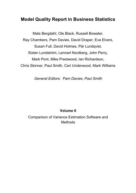
<strong>Model</strong> <strong>Quality</strong> <strong>Report</strong> <strong>in</strong> Bus<strong>in</strong>ess <strong>Statistics</strong><br />
Mats Bergdahl, Ole Black, Russell Bowater,<br />
Ray Chambers, Pam Davies, David Draper, Eva Elvers,<br />
Susan Full, David Holmes, Pär Lundqvist,<br />
Sixten Lundström, Lennart Nordberg, John Perry,<br />
Mark Pont, Mike Prestwood, Ian Richardson,<br />
Chris Sk<strong>in</strong>ner, Paul Smith, Ceri Underwood, Mark Williams<br />
General Editors: Pam Davies, Paul Smith<br />
Volume II<br />
Comparison of Variance Estimation Software and<br />
Methods
Preface<br />
The <strong>Model</strong> <strong>Quality</strong> <strong>Report</strong> <strong>in</strong> Bus<strong>in</strong>ess <strong>Statistics</strong> project was set up to develop a detailed<br />
description of the methods for assess<strong>in</strong>g the quality of surveys, with particular application <strong>in</strong><br />
the context of bus<strong>in</strong>ess surveys, and then to apply these methods <strong>in</strong> some example surveys to<br />
evaluate their quality. The work was specified and <strong>in</strong>itiated by Eurostat follow<strong>in</strong>g on from the<br />
Work<strong>in</strong>g Group on <strong>Quality</strong> of Bus<strong>in</strong>ess Statsitics. It was funded by Eurostat under SUP-COM<br />
1997, lot 6, and has been undertaken by a consortium of the UK Office for National<br />
<strong>Statistics</strong>, <strong>Statistics</strong> Sweden, the University of Southampton and the University of Bath, with<br />
the Office for National <strong>Statistics</strong> manag<strong>in</strong>g the contract.<br />
The report is divided <strong>in</strong>to four volumes, of which this is the second. This volume deals with<br />
the software available for variance estimation <strong>in</strong> sample surveys, compar<strong>in</strong>g a range of<br />
packages and methods, and evaluat<strong>in</strong>g some of their properties through a simulation study<br />
us<strong>in</strong>g a known population<br />
Other volumes of the report conta<strong>in</strong>:<br />
• a review and development of the theory and methods for assess<strong>in</strong>g quality <strong>in</strong> bus<strong>in</strong>ess<br />
surveys (volume I);<br />
• example assessments of quality for an annual and a monthly bus<strong>in</strong>ess survey from<br />
Sweden and the UK (volume III);<br />
• guidel<strong>in</strong>es for and experiences of implement<strong>in</strong>g the methods (volume IV).<br />
An outl<strong>in</strong>e of the chapters <strong>in</strong> the report is given on the follow<strong>in</strong>g pages.<br />
Acknowledgements<br />
Apart from the authors, several other people have made large contributions without which<br />
this report would not have reached its current form. In particular we would like to mention<br />
Tim Jones, Anita Ullberg, Jeff Evans, Trevor Fenton, Jonathan Gough, Dan Hedl<strong>in</strong>, Sue<br />
Hibbitt and Steve James, and we would also like to thank all the other people who have been<br />
so helpful and understand<strong>in</strong>g while our attention has been focussed on this project!
Outl<strong>in</strong>e of <strong>Model</strong> <strong>Quality</strong> <strong>Report</strong> Volumes<br />
Volume I<br />
1. Methodology overview and <strong>in</strong>troduction<br />
Part 1: Sampl<strong>in</strong>g errors<br />
2. Probability sampl<strong>in</strong>g: basic methods<br />
3. Probability sampl<strong>in</strong>g: extensions<br />
4. Sampl<strong>in</strong>g errors under non-probability sampl<strong>in</strong>g<br />
Part 2: Non-sampl<strong>in</strong>g errors<br />
5. Frame errors<br />
6. Measurement errors<br />
7. Process<strong>in</strong>g errors<br />
8. Non-response errors<br />
9. <strong>Model</strong> assumption errors<br />
Part 3: Other aspects of quality<br />
10. Comparability and coherence<br />
Part 4: Conclusions and References<br />
11. Conclud<strong>in</strong>g remarks<br />
12. References<br />
Volume II<br />
1. Introduction<br />
2. Evaluation of variance estimation software<br />
3. Simulation study of alternative variance estimation methods<br />
4. Variances <strong>in</strong> STATA/SUDAAN compared with analytic variances<br />
5. References<br />
Volume III<br />
1. Introduction<br />
Part 1: Annual statistics<br />
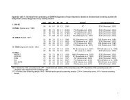
2. <strong>Quality</strong> assessment of the 1995 Swedish Annual Production Volume Index<br />
3. <strong>Quality</strong> assessment of the 1996 UK Annual Production and Construction Inquiries<br />
Part 2: Short-term statistics<br />
4. <strong>Quality</strong> assessment of the Swedish Short-term Production Volume Index<br />
5. <strong>Quality</strong> assessment of the UK Index of Production<br />
6. <strong>Quality</strong> assessment of the UK Monthly Production Inquiry<br />
Part 3: The UK’s Sampl<strong>in</strong>g Frame<br />
7. Sampl<strong>in</strong>g frame for the UK
Volume IV<br />
1. Introduction<br />
2. Guidel<strong>in</strong>es on implementation<br />
3. Implementation report for Sweden<br />
4. Implementation report for the UK<br />
5. Visit to Statistisches Bundesamt, Wiesbaden, Germany, 23-24 March 1998<br />
6. Visit to CSO, Cork, Ireland, 23 April 1998<br />
7. Visit to INE, Madrid, SPa<strong>in</strong>, 6 July 1998
Contents<br />
1 Introduction ..............................................................................................................................................2<br />
2 Evaluation of variance estimation software..............................................................................................4<br />
2.1 Requirements on software for bus<strong>in</strong>ess statistics.................................................................................4<br />
2.1.1 Introduction.....................................................................................................................................4<br />
2.1.2 Parameters.......................................................................................................................................4<br />
2.1.3 Po<strong>in</strong>t estimators...............................................................................................................................5<br />
2.1.4 Variance estimation methods ..........................................................................................................9<br />
2.1.4.1 The Taylor l<strong>in</strong>earisation method............................................................................................9<br />
2.1.4.2 The Jackknife method..........................................................................................................10<br />
2.1.4.3 The Bootstrap method..........................................................................................................10<br />
2.1.4.4 The Balanced Repeated Replication (BRR) method............................................................10<br />
2.1.5 Summary of requirements .............................................................................................................10<br />
2.2 Critical comparison of software packages .........................................................................................11<br />
2.2.1 Sample designs..............................................................................................................................12<br />
2.2.2 Nonresponse models and outlier treatment ...................................................................................13<br />
2.2.3 Parameters.....................................................................................................................................14<br />
2.2.4 Estimators......................................................................................................................................15<br />
2.2.5 Variance estimators.......................................................................................................................16<br />
2.2.6 Interfaces, documentation and help...............................................................................................18<br />
2.2.6.1 Initial reactions of new users to the software.......................................................................21<br />
2.2.7 Correctness and speed ...................................................................................................................21<br />
2.2.8 Ease of <strong>in</strong>tegration with process<strong>in</strong>g systems .................................................................................21<br />
2.2.9 Costs..............................................................................................................................................22<br />
2.3 Recommendations for variance estimation software for use <strong>in</strong> EU member states ...........................22<br />
3 Simulation study of alternative variance estimation methods.................................................................24<br />
3.1 The simulated population...................................................................................................................24<br />
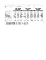
3.1.1 A model for data generation..........................................................................................................24<br />
3.1.2 Doma<strong>in</strong>s and estimators ................................................................................................................25<br />
3.1.3 Data features..................................................................................................................................25<br />
3.2 Process<strong>in</strong>g ..........................................................................................................................................26<br />
3.3 Results................................................................................................................................................26<br />
3.3.1 Comparison of estimators..............................................................................................................26<br />
3.3.2 Comparison of variance estimators ...............................................................................................27<br />
3.3.2.1 Naïve variance estimators....................................................................................................29<br />
3.3.3 Comparison of software package outputs......................................................................................30<br />
3.4 General conclusions ...........................................................................................................................31<br />
4 Variances <strong>in</strong> STATA/SUDAAN compared with analytical variances....................................................33<br />
4.1 Expansion estimator...........................................................................................................................33<br />
4.2 Ratio estimator...................................................................................................................................33<br />
4.3 What does SUDAAN do ..................................................................................................................34<br />
5 References ..............................................................................................................................................36<br />
i
1 Introduction<br />
Paul Smith, Office for National <strong>Statistics</strong><br />
One of the key <strong>in</strong>dicators of quality <strong>in</strong> sample surveys is the sampl<strong>in</strong>g variance aris<strong>in</strong>g from<br />
the random sampl<strong>in</strong>g mechanism through the randomisation distribution. This <strong>in</strong>dicates the<br />
variability <strong>in</strong>troduced by choos<strong>in</strong>g a sample <strong>in</strong>stead of enumerat<strong>in</strong>g the whole population,<br />
assum<strong>in</strong>g that the <strong>in</strong>formation collected <strong>in</strong> the survey is otherwise exactly correct. For a<br />
discussion of the theory underly<strong>in</strong>g these calculations, see chapters M2 1 and M3 of the<br />
methodology report (volume I). For any given survey, an estimator of this sampl<strong>in</strong>g variance<br />
can be evaluated and used to <strong>in</strong>dicate the accuracy of the estimates. The forms of these<br />
estimators are often complex, especially when the design conta<strong>in</strong>s strata or clusters, and when<br />
the estimation model uses auxiliary <strong>in</strong>formation to improve the accuracy.<br />
In order to make these calculations feasible, appropriate software is required, and although it<br />
is possible to construct a program with<strong>in</strong> most survey process<strong>in</strong>g systems to do this for a<br />
specific survey, there has been a recent trend towards the production of generalised software<br />
which will calculate the appropriate variances <strong>in</strong> a wide range of commonly met survey<br />
situations. These must then be <strong>in</strong>corporated <strong>in</strong>to the survey process. Sampl<strong>in</strong>g variances are<br />
often not time-critical <strong>in</strong>formation, and any difficulties with data transfer to or setup of this<br />
software are offset by the generalised nature of the programs.<br />
In this paper we evaluate five generalised packages which are publicly available: CLAN,<br />
GES, SUDAAN, STATA and WesVar PC. There are four ma<strong>in</strong> variance estimation methods,<br />
Taylor, jackknife, bootstrap and balanced repeated replication (these are expla<strong>in</strong>ed <strong>in</strong> section<br />
2.1.4), and between them these packages cover all the available methods except the bootstrap<br />
(Table 1.1). These are the packages which were available at the time of putt<strong>in</strong>g together the<br />
tender for this study, with the exception of PC-CARP which was available but has not been<br />
studied. Other packages are be<strong>in</strong>g developed; those known to the <strong>Model</strong> <strong>Quality</strong> <strong>Report</strong> team are<br />
BASCULA and POULPE but neither of these seems to be fully functional <strong>in</strong> its current version.<br />
Method<br />
Direct + Taylor<br />
series methods<br />
Jackknife Bootstrap Balanced<br />
repeated<br />
replication<br />
Software<br />
CLAN<br />
GES<br />
STATA<br />
SUDAAN<br />
GES<br />
SUDAAN<br />
WesVarPC<br />
None<br />
SUDAAN<br />
WesVarPC<br />
Table 1.1: Variance estimation methods available <strong>in</strong> the evaluated software packages.<br />
1 Reference is made throughout this document to the Methodology report by prefix<strong>in</strong>g section references with an<br />
“M”.<br />
2
The requirements for a variance estimation package are discussed <strong>in</strong> section 2.1, and there is<br />
a comparative description of the packages <strong>in</strong> section 2.2. Section 2.3 draws conclusions about<br />
the suitability of the packages for general use <strong>in</strong> bus<strong>in</strong>ess surveys <strong>in</strong> EU member states, and<br />
makes recommendations for which should be adopted. A separate simulation study has been<br />
undertaken to look at the properties of the available variance estimators, and this is presented<br />
<strong>in</strong> chapter 3 of this report. A more detailed description of the differences <strong>in</strong> underly<strong>in</strong>g<br />
methods between STATA/SUDAAN and the other packages for the Taylor l<strong>in</strong>earisation<br />
approach to ratio estimation is given <strong>in</strong> chapter 4.<br />
3
2 Evaluation of variance estimation software<br />
Paul Smith, Office for National <strong>Statistics</strong><br />
Sixten Lundström, <strong>Statistics</strong> Sweden<br />
Ceri Underwood, Office for National <strong>Statistics</strong><br />
2.1 Requirements on software for bus<strong>in</strong>ess statistics<br />
2.1.1 Introduction<br />
The units <strong>in</strong> bus<strong>in</strong>ess surveys can be of various types, such as enterprises and k<strong>in</strong>d-of-activity<br />
units. Mostly a Bus<strong>in</strong>ess Register (BR) is used as the frame for the survey. There is a set of<br />
units on the BR, such as enterprises, legal units, local units, and possibly k<strong>in</strong>d-of-activity<br />
units. There is a set of variables for each type of unit, some common to other types of unit,<br />
some unique. Ord<strong>in</strong>arily, the BR conta<strong>in</strong>s <strong>in</strong>formation on which <strong>in</strong>dustry each unit belongs to<br />
and a measure of the “size” of the unit. The size variable is often the number of employees, or<br />
perhaps a measure of turnover (depend<strong>in</strong>g on unit level). These variables and their reference<br />
dates affect the use of auxiliary <strong>in</strong>formation <strong>in</strong> the sampl<strong>in</strong>g design and <strong>in</strong> the estimation<br />
process.<br />
In bus<strong>in</strong>ess surveys two typical k<strong>in</strong>ds of probability sampl<strong>in</strong>g design can be identified,<br />
namely (i) one-step element and (ii) one-step cluster. Typical examples are (i) surveys with<br />
the enterprise as both the sampl<strong>in</strong>g unit and observation unit, and (ii) surveys with the<br />
enterprise as the sampl<strong>in</strong>g unit and all its k<strong>in</strong>d-of-activity units or all its local units as the<br />
observation units.<br />
The population is often stratified by <strong>in</strong>dustry and size, and from each stratum a simple<br />
random sample is drawn. The stratification variable ‘<strong>in</strong>dustry’ is used with regard to the<br />
doma<strong>in</strong>s of estimation that are mostly def<strong>in</strong>ed by <strong>in</strong>dustry. Size is usually an effective<br />
variable for reduc<strong>in</strong>g the sampl<strong>in</strong>g variability (see chapter M2).<br />
Bus<strong>in</strong>ess surveys are ord<strong>in</strong>arily carried out cont<strong>in</strong>uously, either annually, quarterly or<br />
monthly. The samples may be co-ord<strong>in</strong>ated over time, us<strong>in</strong>g a panel system or possibly a<br />
technique based on permanent random numbers (Ohlsson 1995). Units <strong>in</strong> bus<strong>in</strong>ess statistics<br />
typically change fairly rapidly; they can “die”, they can merge with another unit and they can<br />
split <strong>in</strong>to several units. The <strong>in</strong>dustrial classification may change, and the size of the unit can<br />
vary.<br />
2.1.2 Parameters<br />
Let us look at the various types of f<strong>in</strong>ite population parameters that are typical for a bus<strong>in</strong>ess<br />
survey. Consider the f<strong>in</strong>ite population of N units U { u u u }<br />
<strong>in</strong>terested <strong>in</strong> the population total<br />
t<br />
y<br />
=<br />
1<br />
,..., ,..., . Sometimes we are<br />
k<br />
= ∑ y<br />
(2.1)<br />
U<br />
k<br />
N<br />
4
where y k<br />
is the value of the study variable, y, for the kth element. Moreover, totals for<br />
doma<strong>in</strong>s – typically <strong>in</strong>dustries – are also common. Let us denote the doma<strong>in</strong> set by U d<br />
,<br />
d = 1,..., D, and set y<br />
( d) k=<br />
⎧yk<br />
if unit k ∈U<br />
⎨<br />
⎩0<br />
otherwise<br />
5<br />
d<br />
. Then the total for doma<strong>in</strong> d is<br />
ty<br />
= ∑U<br />
y( d) k<br />
= ∑U<br />
yk<br />
(2.2)<br />
d<br />
Ratios of different types are common <strong>in</strong> bus<strong>in</strong>ess statistics. To def<strong>in</strong>e these types let z be<br />
another study variable and let the population total for z be denoted t z<br />
and the doma<strong>in</strong> total<br />
t zd<br />
. One type of ratio is<br />
d<br />
y d z d<br />
d<br />
R = t t<br />
(2.3)<br />
A typical example here is production per head with <strong>in</strong>dustry as doma<strong>in</strong>. Another type of ratio<br />
is<br />
R = t y<br />
t y<br />
(2.4)<br />
show<strong>in</strong>g for example the production of an <strong>in</strong>dustry, relative to the whole population.<br />
Another parameter of <strong>in</strong>terest is<br />
d<br />
d<br />
I = t t′<br />
(2.5)<br />
y d z d<br />
where ‘prime’ (′) <strong>in</strong>dicates ‘relative to another population’. A typical application of (2.5) is<br />
the relative change <strong>in</strong> production (say) by <strong>in</strong>dustry from one period to another, that is, the<br />
totals <strong>in</strong> the numerator and the denom<strong>in</strong>ator have different reference times, but otherwise<br />
relate to the same variable and doma<strong>in</strong>. The sample units (<strong>in</strong>volved <strong>in</strong> the numerator and<br />
denom<strong>in</strong>ator) are partly the same, partly different, and units that contribute to the total on<br />
both occasions may have changed doma<strong>in</strong> (<strong>in</strong>dustry) <strong>in</strong> between.<br />
Indices of production (say) are examples of complex sets of parameters, typically built up<br />
from components like (2.5), and usually also deflated by price <strong>in</strong>dices. Yet (2.5) is already a<br />
challenge for the available software. The complexity also depends on the way samples are coord<strong>in</strong>ated<br />
over time.<br />
2.1.3 Po<strong>in</strong>t estimators<br />
To estimate the parameters def<strong>in</strong>ed <strong>in</strong> section 2.1.2, a sample s of size n is drawn from U (or<br />
actually from the frame). Stratification is commonly used <strong>in</strong> bus<strong>in</strong>ess surveys, that is, a<br />
simple random sample s h<br />
of size n h<br />
is drawn from the stratum U h<br />
, h = 1,..., H , where<br />
U<br />
=<br />
for k<br />
H<br />
U h<br />
h=1<br />
U . Let the stratum sizes be N h<br />
, h = 1,..., H , and the design weights are d<br />
k<br />
= N<br />
h<br />
nh<br />
∈ s h<br />
.<br />
However, nonresponse occurs <strong>in</strong> the survey process, and the response set r of size m is<br />
obta<strong>in</strong>ed, where r ⊆ s. There are two ma<strong>in</strong> ways of treat<strong>in</strong>g this problem, namely weight<strong>in</strong>g<br />
and imputation. In weight<strong>in</strong>g, the nonresponse compensation adjustment weight v k<br />
is
constructed primarily with the aim of reduc<strong>in</strong>g the nonresponse bias, but is also used to<br />
reduce the additional component of sampl<strong>in</strong>g error caused by nonresponse (see chapter M8).<br />
When us<strong>in</strong>g the weight<strong>in</strong>g approach the estimator consists of the sum of the weighted values<br />
for elements <strong>in</strong> r, where the weight consists of the product of d k<br />
and v k<br />
, where v k<br />
is the tool<br />
for mak<strong>in</strong>g the <strong>in</strong>ference from r to s and d k<br />
from s to U. When imputation is used, values for<br />
all n elements are used <strong>in</strong> the estimation, but now n-m of these values are estimates<br />
(approximations) of the real values.<br />
None of these methods is expected to completely elim<strong>in</strong>ate the bias. When a substantial<br />
nonresponse bias is still present the variance estimate and the confidence <strong>in</strong>terval will be an<br />
unrelevant and <strong>in</strong>complete measure of the quality of the po<strong>in</strong>t estimate. As <strong>in</strong>dicated above,<br />
nonresponse will also cause an additional component of sampl<strong>in</strong>g error. This is obvious <strong>in</strong><br />
weight<strong>in</strong>g, s<strong>in</strong>ce the number of observations is reduced from n to m.<br />
In the follow<strong>in</strong>g, we describe estimators used <strong>in</strong> bus<strong>in</strong>ess surveys. Here we describe the<br />
estimator us<strong>in</strong>g a nonresponse compensation adjustment weight, which has a more complex<br />
form than the estimator based on imputation.<br />
The nonresponse compensation adjustment weight is an approximation of the <strong>in</strong>verse of the<br />
response probability. That is, one seeks a relevant model of the response probabilities.<br />
Commonly, this model consists of a group<strong>in</strong>g of the sample s. Särndal, Swensson & Wretman<br />
(1992) denote them Response Homogeneity Groups (RHGs). In the follow<strong>in</strong>g we will choose<br />
among three different types of RHGs, namely<br />
(i)<br />
(ii)<br />
(iii)<br />
strata and RHGs co<strong>in</strong>cide<br />
RHGs are subgroups of strata<br />
RHGs cut across the strata<br />
⎫<br />
⎪<br />
⎬<br />
⎪<br />
⎭<br />
(2.6)<br />
The simplest estimator is the Horvitz-Thompson estimator, comb<strong>in</strong>ed with nonresponse<br />
model (i). That means that we f<strong>in</strong>d it plausible that each sampled element <strong>in</strong> the stratum<br />
responds with the same probability. In this case the nonresponse compensation weight is<br />
nh<br />
vk<br />
= and s<strong>in</strong>ce d<br />
k<br />
= N<br />
h<br />
nh<br />
the result<strong>in</strong>g weight is N<br />
h<br />
mh<br />
and the estimator has the<br />
mh<br />
form<br />
H<br />
$t = ∑ N y<br />
y h rh<br />
h=1<br />
(2.7)<br />
where y<br />
rh<br />
1<br />
= ∑<br />
m<br />
h<br />
rh<br />
y<br />
k<br />
.<br />
A somewhat more complex estimator is obta<strong>in</strong>ed when us<strong>in</strong>g nonresponse model (ii), namely<br />
$t<br />
y<br />
H N Lh<br />
h<br />
= ∑ ∑ n<br />
h= 1 n q=<br />
1<br />
h<br />
hq<br />
y<br />
rhp<br />
(2.8)<br />
6
where n hq<br />
is the size of the part of s that falls <strong>in</strong>to RHG hq; m hq<br />
is the size of r hq<br />
, the<br />
response set <strong>in</strong> RHG hq, and y<br />
r<br />
hp<br />
1<br />
= ∑<br />
m<br />
hp<br />
r<br />
hp<br />
y<br />
k<br />
When us<strong>in</strong>g nonresponse model (iii) an even more complex estimator is obta<strong>in</strong>ed. Let us here<br />
express it by the general version<br />
.<br />
$t = ∑ d v y<br />
(2.9)<br />
y r k k k<br />
Frames used <strong>in</strong> the Member States regularly conta<strong>in</strong> more <strong>in</strong>formation than <strong>in</strong>dustry and<br />
number of employees, for example, the turnover from a previous time of reference.<br />
Moreover, geographical <strong>in</strong>formation for the local units is commonly available. Thus, there<br />
may be register <strong>in</strong>formation, which is correlated with the study variables and/or the response<br />
probabilities, but not used <strong>in</strong> the estimator of the form (2.9). A simple version of such<br />
<strong>in</strong>formation is a partition of the population. To demonstrate estimators based on such a<br />
partition we let U ,..., U ,..., U be groups that form a mutually exclusive and exhaustive<br />
1<br />
p<br />
P<br />
partition of the population. Assume that we know the sizes of these groups, N1,..., Np,..., NP.<br />
Then they can be used as poststrata. Such an estimator, us<strong>in</strong>g the nonresponse model (i)<br />
mentioned above, has the form<br />
t$<br />
yr<br />
P N<br />
p<br />
H N<br />
h<br />
= ∑<br />
r<br />
N$<br />
∑ ∑ y<br />
p h m<br />
hp<br />
= 1 = 1<br />
p<br />
h<br />
k<br />
(2.10)<br />
with N$ = ∑ N$<br />
p<br />
H<br />
h=1<br />
hp<br />
, where $ N<br />
to the union of U h<br />
and U p<br />
.<br />
hp<br />
N<br />
h<br />
=<br />
m m hp<br />
; m hp<br />
is the size of r hp<br />
, the response set that belongs<br />
h<br />
Estimator (2.10) is a special case of the follow<strong>in</strong>g general estimator<br />
where<br />
$t = ∑ d v g y<br />
(2.11)<br />
yr r k k k k<br />
g<br />
k<br />
T<br />
T 2 −1<br />
2<br />
( ∑ x ) ( / )<br />
U<br />
−∑ d<br />
r kvk<br />
x<br />
k<br />
k ∑ d<br />
r kvk<br />
x<br />
k<br />
x<br />
k<br />
σ<br />
k<br />
x<br />
k<br />
σ<br />
= (2.12)<br />
1+<br />
k<br />
2<br />
By choos<strong>in</strong>g the positive factors σ k<br />
the approach can be made very flexible. This will<br />
become apparent <strong>in</strong> subsequent sections. The vector x<br />
k<br />
is called the auxiliary vector <strong>in</strong> what<br />
follows. Estimator (2.11) is based on a general approach to regression for two-phase<br />
sampl<strong>in</strong>g follow<strong>in</strong>g Särndal & Swensson (1987). It is here used <strong>in</strong> the nonresponse situation,<br />
but s<strong>in</strong>ce we do not know the response probabilities the second-phase <strong>in</strong>clusion probabilities<br />
have to be estimated <strong>in</strong> some way (see also M2.3.1.5). The <strong>in</strong>verse of this estimate is denoted<br />
by v k<br />
. In what follows the estimator (2.11) is called the GREG estimator.<br />
7
In the case of poststratification the auxiliary vector is def<strong>in</strong>ed by x = ( γ γ γ ) T<br />
k<br />
1 k<br />
,...,<br />
pk<br />
,...,<br />
Pk<br />
⎧1 if unit k ∈U<br />
p<br />
2<br />
where, for p = 1,..., P,<br />
γ<br />
pk<br />
= ⎨<br />
and σ k<br />
= 1 for all k. This poststratification<br />
⎩0<br />
otherwise<br />
approach gives us one simple method of deal<strong>in</strong>g with outly<strong>in</strong>g observations <strong>in</strong> a survey, s<strong>in</strong>ce<br />
they can be moved <strong>in</strong>to an appropriate poststratum for estimation.<br />
Most of the classical estimators can be derived as special cases from the GREG estimator.<br />
For example, if x<br />
k<br />
= xk<br />
for all k and σ 2 k<br />
∝ x k<br />
, where x k<br />
is a cont<strong>in</strong>uous variable, and when<br />
nonresponse model (i) is used, then the follow<strong>in</strong>g estimator is obta<strong>in</strong>ed:<br />
$t<br />
yr<br />
=<br />
H<br />
∑ N y<br />
h=<br />
1<br />
H<br />
h<br />
∑ N x<br />
h=<br />
1<br />
h<br />
rh<br />
rh<br />
∑<br />
U<br />
x<br />
k<br />
(2.13)<br />
Estimator (2.13) is sometimes called the comb<strong>in</strong>ed ratio estimator.<br />
Sometimes the group totals ∑U<br />
p<br />
x<br />
k<br />
are known and, <strong>in</strong> this general case, the p-groups are<br />
called model groups. Let us present a simple example. As before assume that x k<br />
is a<br />
cont<strong>in</strong>uous variable, but here we know the quantities ∑ ; p = 1,..., P. Let<br />
( γ x γ x γ x ) T<br />
x<br />
k<br />
=<br />
1 k k<br />
,...,<br />
pk k<br />
,...,<br />
Pk k<br />
, σ 2 k<br />
∝ x k<br />
for each p-group, and the RHGs co<strong>in</strong>cide with<br />
strata (nonresponse model (i)) then the GREG estimator takes the form<br />
U p<br />
x k<br />
t$<br />
yr<br />
=<br />
H<br />
$<br />
P<br />
∑ N<br />
h=<br />
1<br />
∑<br />
H<br />
p=<br />
1<br />
∑ N$<br />
h=<br />
1<br />
hp<br />
hp<br />
y<br />
x<br />
rhp<br />
rhp<br />
∑<br />
U p<br />
x<br />
k<br />
(2.14)<br />
If strata and model groups co<strong>in</strong>cide then estimator (2.14) can be written<br />
$t<br />
yr<br />
H yr<br />
h<br />
= ∑ ∑<br />
h=1<br />
x<br />
r<br />
h<br />
U<br />
h<br />
x<br />
k<br />
(2.15)<br />
Estimator (2.15) is sometimes called the separate ratio estimator.<br />
When x<br />
k<br />
= ( 1, xk<br />
) for all k and σ<br />
2 k<br />
= constant , then the classical regression estimator is<br />
obta<strong>in</strong>ed.<br />
Many bus<strong>in</strong>ess surveys are subject to occasional unusual observations, or outliers, which can<br />
have a large effect on the estimates. In these cases, robust versions of po<strong>in</strong>t estimators are<br />
often used, with the simplest be<strong>in</strong>g the poststratification estimator with the outliers <strong>in</strong> their<br />
own (completely enumerated) poststratum. This follows from the method above (2.13). Other<br />
methods <strong>in</strong>volve adjust<strong>in</strong>g the weights or the respond<strong>in</strong>g values, and w<strong>in</strong>sorisation is<br />
becom<strong>in</strong>g widely used with<strong>in</strong> the UK for treat<strong>in</strong>g outliers. This leads to a different estimator,<br />
which does not necessarily fit completely <strong>in</strong>to the GREG framework.<br />
8
The parameters (2.1)-(2.4) are totals or functions of totals from the same period of reference.<br />
Estimators for these parameters can be obta<strong>in</strong>ed by replac<strong>in</strong>g these totals by their estimators.<br />
Parameter (2.5) is much more complex s<strong>in</strong>ce it conta<strong>in</strong>s totals from two periods of reference.<br />
In most surveys two consecutive samples are drawn <strong>in</strong> such a way that they overlap each<br />
other. That makes it possible to construct comb<strong>in</strong>ed estimators that are more effective than<br />
just replac<strong>in</strong>g the totals by their estimators. However, variance estimation becomes<br />
complicated. We do not go deeper <strong>in</strong>to this problem but just refer to Nordberg (1998), who<br />
has found a solution to the special sampl<strong>in</strong>g procedure used at <strong>Statistics</strong> Sweden.<br />
So far we have only discussed one-step element sampl<strong>in</strong>g designs, but it is easy to see how<br />
the one-step cluster alternative affects the formulas. Auxiliary <strong>in</strong>formation can be known at<br />
the cluster level or at the unit level. In the latter case we can choose to use the auxiliary<br />
<strong>in</strong>formation either at cluster level or at unit level. When the auxiliary <strong>in</strong>formation is known<br />
only at the cluster level the model groups are, of course, def<strong>in</strong>ed for that level.<br />
2.1.4 Variance estimation methods<br />
There are four pr<strong>in</strong>cipal ways of calculat<strong>in</strong>g variances (Wolter 1985), each unbiassed or<br />
asymptotically unbiassed <strong>in</strong> most widely-used design-estimation strategies if full response is<br />
assumed, but each (<strong>in</strong> general) produc<strong>in</strong>g a different value for the unbiassed estimate:<br />
• direct calculation and Taylor l<strong>in</strong>earisation;<br />
• jackknife;<br />
• bootstrap;<br />
• balanced repeated replication method.<br />
Before we discuss these methods just a few words about variance estimation when imputation<br />
is used, follow<strong>in</strong>g the discussion <strong>in</strong> section 2.1.3. The literature describes many imputation<br />
methods such as nearest neighbour donor, current ratio, current mean, auxiliary trend, etc.<br />
However, the theoretical development of variance estimators when data conta<strong>in</strong> imputations<br />
is still <strong>in</strong> its <strong>in</strong>itial phase. Two examples of articles on this problem are Särndal (1992) and<br />
Deville & Särndal (1994). In surveys where the ‘complete data set’ is treated as if it were the<br />
full-response set, however, this will commonly underestimate the variance (see, for example,<br />
Rub<strong>in</strong> 1986).<br />
2.1.4.1 The Taylor l<strong>in</strong>earisation method<br />
Direct calculation <strong>in</strong>volves application of (normally) the Sen-Yates-Grundy estimator (Sen<br />
1953, Yates & Grundy 1953) to form the variances of simple survey estimates. More<br />
complex survey estimates are first l<strong>in</strong>earised by tak<strong>in</strong>g the first-order terms <strong>in</strong> an appropriate<br />
Taylor-series expansion, and then the SYG estimates are <strong>in</strong>serted <strong>in</strong>to the l<strong>in</strong>earised formula.<br />
This is basically a set of appropriate l<strong>in</strong>ear expressions for the variances of estimators, which<br />
has to be coded <strong>in</strong>to the software. Every different design-estimand 2 comb<strong>in</strong>ation requires a<br />
different formula which must be (essentially) hard-coded; separate formulae are not required<br />
for different estimation models if the GREG estimator (see equation (2.11)) is present, as all<br />
the commonly used models are either GREG or special cases of it.<br />
9
2.1.4.2 The Jackknife method<br />
The jackknife <strong>in</strong>volves dropp<strong>in</strong>g an observation and recalculat<strong>in</strong>g the estimates from the<br />
rema<strong>in</strong><strong>in</strong>g observations, repeat<strong>in</strong>g successively until all observations have been dropped, and<br />
then f<strong>in</strong>d<strong>in</strong>g the variance of the result<strong>in</strong>g series of estimates (with a suitable multiplier to give<br />
approximate unbiassedness). The drop-one jackknife is usually used, as it can be shown to<br />
give the variance estimate with the smallest sampl<strong>in</strong>g variability, although it is possible to<br />
drop pairs of observations (or even more) too; this strategy is usually adopted to speed up<br />
process<strong>in</strong>g s<strong>in</strong>ce drop-one is the most processor-<strong>in</strong>tensive method. We consider only dropone<br />
methods here. More <strong>in</strong>formation on the jackknife estimator is <strong>in</strong> M2.4.2.2-M2.4.2.3.<br />
It should be noted that the jackknife is only strictly applicable <strong>in</strong> with-replacement designs. It<br />
can be used <strong>in</strong> without-replacement designs where the sampl<strong>in</strong>g fractions are “sufficiently<br />
small” (Wolter 1985, p168), but <strong>in</strong> many bus<strong>in</strong>ess survey designs, the sampl<strong>in</strong>g fractions are<br />
relatively large. The dangers of this approach are illustrated <strong>in</strong> the simulation <strong>in</strong> chapter 3<br />
below.<br />
2.1.4.3 The Bootstrap method<br />
The bootstrap <strong>in</strong>volves resampl<strong>in</strong>g a number of times with replacement from the sampled<br />
observations, and calculat<strong>in</strong>g an estimate for each of the bootstrap samples. The variance of<br />
these “bootstrap” estimates is then calculated, aga<strong>in</strong> with a suitable multiplier to ensure<br />
unbiassedness. The method is described <strong>in</strong> more detail <strong>in</strong> M2.4.2.4.<br />
2.1.4.4 The Balanced Repeated Replication (BRR) method<br />
This is derived from the balanced half samples (BHS) method which has a very specific<br />
application <strong>in</strong> cluster designs where each cluster has exactly two f<strong>in</strong>al stage units. By<br />
successively delet<strong>in</strong>g one of these units and chang<strong>in</strong>g the weight of the other to compensate, a<br />
range of estimates can be produced whose variance can be calculated and suitably adjusted to<br />
give an appropriate variance estimator (Wolter 1985). Various adaptations of this can be<br />
applied <strong>in</strong> designs where the clusters have variable numbers of units, based on divid<strong>in</strong>g these<br />
<strong>in</strong>to two groups. Recent research (Rao & Shao 1996) shows that only by us<strong>in</strong>g repeated<br />
divisions (“repeatedly grouped balanced half samples” (RGBHS)) can an asymptotically<br />
correct estimator be obta<strong>in</strong>ed. This method, then, can only be used for the usual stratified<br />
designs <strong>in</strong> bus<strong>in</strong>ess surveys if we are prepared to treat a stratum as if it were a cluster, and to<br />
run the package a number of times with different divisions of the elements <strong>in</strong>to two groups;<br />
where there is an odd number of elements <strong>in</strong> the stratum the results are biassed, and ways of<br />
reduc<strong>in</strong>g this bias (but not elim<strong>in</strong>at<strong>in</strong>g it) are described <strong>in</strong> Slootbeek (1998). There are ways<br />
<strong>in</strong> which this can be done, but the results are typically unsatisfactory and the manipulation of<br />
both data and software becomes very <strong>in</strong>volved.<br />
2.1.5 Summary of requirements<br />
There is a number of requirements for po<strong>in</strong>t and variance estimation <strong>in</strong> bus<strong>in</strong>ess surveys<br />
which any software should satisfy. We have po<strong>in</strong>ted out several such requirements <strong>in</strong> the<br />
2 th<strong>in</strong>g to be estimated<br />
10
previous sections. However, <strong>in</strong> order to simplify the evaluation we will here present a<br />
structured summary of these requirements. The demands on the software will certa<strong>in</strong>ly vary<br />
between Member States (MS). Consequently, packages which only meet some of the<br />
requirements mentioned ahead may be sufficient for a particular MS, provided that they meet<br />
the requirements of this MS.<br />
The packages will be evaluated with respect to their ability to cope with the follow<strong>in</strong>g<br />
situations.<br />
Sampl<strong>in</strong>g designs: One-step stratified sampl<strong>in</strong>g of units or clusters. In each stratum a simple<br />
random sample is drawn. In some strata the f<strong>in</strong>ite population correction (fpc) has a large<br />
effect; <strong>in</strong> take-all strata it reduces the sampl<strong>in</strong>g variance to zero. Panels or random number<br />
techniques are used <strong>in</strong> the sampl<strong>in</strong>g procedure.<br />
Nonresponse models and outlier adjustment: Weight<strong>in</strong>g with<strong>in</strong> RHGs (i)-(iii), as described <strong>in</strong><br />
2.1.3 and equation (2.6) or imputation as described <strong>in</strong> sections 2.1.3 and 2.1.4, and outlier<br />
treatment us<strong>in</strong>g poststratification or w<strong>in</strong>sorisation as described <strong>in</strong> 2.1.3.<br />
Parameters: Parameters for measur<strong>in</strong>g levels as <strong>in</strong> (2.1)-(2.4) and parameters for measur<strong>in</strong>g<br />
change as <strong>in</strong> (2.5). More complex parameters such as <strong>in</strong>dices are also of great <strong>in</strong>terest.<br />
Estimators: Estimators for totals as def<strong>in</strong>ed <strong>in</strong> (2.7) to (2.15). Ratios and other functions of<br />
these estimators are also of <strong>in</strong>terest. Po<strong>in</strong>t estimates and the correspond<strong>in</strong>g variance estimates<br />
for parameters such as (2.5), for example measures of change between two consecutive<br />
periods (a demand<strong>in</strong>g task for the packages) are of <strong>in</strong>terest.<br />
Variance estimators: availability of different variance estimation methods (Taylor, Jackknife,<br />
BRR, Bootstrap).<br />
The packages will also be evaluated with respect to:<br />
• <strong>in</strong>terface, documentation and help functions;<br />
• whether computations are correctly done;<br />
• execution time;<br />
• simplicity to <strong>in</strong>tegrate <strong>in</strong>to production systems;<br />
• cost for purchase or licenses.<br />
2.2 Critical comparison of software packages<br />
The software packages evaluated here fall <strong>in</strong>to two dist<strong>in</strong>ct groups based on the way they are<br />
designed and the type of situations <strong>in</strong> which they can be used. It makes sense to structure the<br />
discussion around these two groups, as the methods employed with<strong>in</strong> the packages are very<br />
similar with<strong>in</strong> groups, and quite different between them.<br />
Group I: CLAN and GES are designed for stratified designs with estimation models up<br />
to the complexity of the generalised regression (GREG) estimator. They are characterised by<br />
hav<strong>in</strong>g two parts to their process<strong>in</strong>g, one <strong>in</strong> which the appropriate weights are calculated for<br />
the survey observations, and then a second phase where the estimates and their associated<br />
variances are produced. The variances specifically take account of these weights, and are<br />
based on the variances of the residuals from the GREG model (or a specific (simpler) case).<br />
11
Group II: STATA, SUDAAN and WesVar are designed pr<strong>in</strong>cipally for cluster designs<br />
with versions of the Horvitz-Thompson (HT) estimator (<strong>in</strong> most cases optionally <strong>in</strong>volv<strong>in</strong>g<br />
poststratification); the key here is that GREG-type estimators (<strong>in</strong>clud<strong>in</strong>g most of the simpler<br />
cases such as ratio and regression estimation) are not supported. STATA and SUDAAN both<br />
work <strong>in</strong> a straightforward way with stratified designs, but WesVar needs clusters at the<br />
penultimate sampl<strong>in</strong>g stage <strong>in</strong> order to work effectively (ma<strong>in</strong>ly because of the BRR variance<br />
estimation method employed). This group is characterised by not hav<strong>in</strong>g a weight calculation<br />
phase and requir<strong>in</strong>g the (HT) weight to be <strong>in</strong>put. In some cases the software can be made to<br />
produce valid or approximately valid results for estimators other than HT, but this is typically<br />
not easy and may require the package to be run more than once for each survey.<br />
2.2.1 Sample designs<br />
CLAN and GES have the follow<strong>in</strong>g designs built-<strong>in</strong>:<br />
1. simple random sampl<strong>in</strong>g;<br />
2. stratified designs;<br />
3. probability proportional to size (with replacement) designs;<br />
4. one stage cluster designs (optionally with the clusters <strong>in</strong> strata).<br />
These cover the ma<strong>in</strong> probability designs used for bus<strong>in</strong>ess surveys <strong>in</strong> Member States, but do<br />
not extend to the more complex designs used <strong>in</strong> some social surveys. It is possible to force<br />
more complex designs through CLAN and GES by accept<strong>in</strong>g some assumptions about<br />
variances at lower stages; one option is to set appropriate jackknife adjustment weights<br />
with<strong>in</strong> GES for two-stage designs. All of these methods, however, are vanish<strong>in</strong>gly rare <strong>in</strong><br />
bus<strong>in</strong>ess surveys, and require considerable expertise and <strong>in</strong>put from the user, so they are not<br />
considered further here. <strong>Statistics</strong> Canada have just begun to develop two-stage cluster<br />
sampl<strong>in</strong>g for <strong>in</strong>clusion <strong>in</strong> the next version of GES (version 5.0).<br />
STATA and SUDAAN have the follow<strong>in</strong>g designs built <strong>in</strong>:<br />
1. simple random sampl<strong>in</strong>g;<br />
2. stratified designs;<br />
3. one stage cluster designs;<br />
4. two- and multi-stage cluster designs.<br />
These cover a wider range of designs, but the complex cluster designs are not typically used<br />
for bus<strong>in</strong>ess surveys, and we know of no examples of their current use <strong>in</strong> bus<strong>in</strong>ess surveys <strong>in</strong><br />
member states. However, this does give some added flexibility <strong>in</strong> the use of the package for<br />
various surveys.<br />
WesVar has the follow<strong>in</strong>g two designs available:<br />
1. simple random sampl<strong>in</strong>g;<br />
2. two-stage cluster designs with exactly two primary sampl<strong>in</strong>g units <strong>in</strong> each cluster.<br />
These designs are very restrictive <strong>in</strong> the context of bus<strong>in</strong>ess surveys where clusters are rarely<br />
used, and where treat<strong>in</strong>g a stratum as if it were a cluster typically gives more then two<br />
primary sampl<strong>in</strong>g units <strong>in</strong> each cluster. For this reason we will not concentrate much<br />
discussion on WesVar.<br />
12
The f<strong>in</strong>ite population correction (fpc) can have a large effect on the variance estimates; with<strong>in</strong><br />
GES and CLAN it is <strong>in</strong>cluded automatically (except for the jackknife estimator <strong>in</strong> GES). In<br />
STATA a specific command option must be used to get the fpc, and <strong>in</strong> SUDAAN it depends<br />
on the design whether the fpc is <strong>in</strong>cluded or not. GES and SUDAAN alike <strong>in</strong>clude the fpc<br />
automatically <strong>in</strong> without-replacement designs, and exclude it <strong>in</strong> with-replacement designs.<br />
However, it can <strong>in</strong> some circumstances be reasonable to use with-replacement variance<br />
estimators as approximate variance estimators <strong>in</strong> without-replacement designs, when<br />
<strong>in</strong>clusion of the fpc can become important; <strong>in</strong>clusion of the fpc is unlikely, however, to solve<br />
all the difficulties of this approach .<br />
2.2.2 Nonresponse models and outlier treatment<br />
CLAN is the only software package to <strong>in</strong>clude the specification of non-response models. This<br />
is done by def<strong>in</strong><strong>in</strong>g response homogeneity groups, which can be def<strong>in</strong>ed differently from the<br />
stratification and model groups, and provide a flexible way of def<strong>in</strong><strong>in</strong>g the weight<strong>in</strong>g<br />
adjustment for non-response <strong>in</strong> l<strong>in</strong>e with equations (2.7)-(2.10). This additional option with<strong>in</strong><br />
CLAN is similar to the sort of methodology which would arise <strong>in</strong> a two-stage stratified<br />
design, with first stage selection be<strong>in</strong>g sampl<strong>in</strong>g from the frame and the second phase be<strong>in</strong>g<br />
“sampl<strong>in</strong>g” respondents from the selected sample. This means that the extra functionality can<br />
be used to make CLAN give appropriate answers <strong>in</strong> some complex designs if there is (or can<br />
be assumed to be) no non-response.<br />
For the other software packages considered here, only two alternatives are available, either to<br />
assume that non-respond<strong>in</strong>g units were not sampled, which is equivalent to imput<strong>in</strong>g their<br />
value with the mean under the estimation model for the stratum <strong>in</strong> which they were selected,<br />
or to fill <strong>in</strong> the miss<strong>in</strong>g values us<strong>in</strong>g some imputation procedure and then use the completed<br />
dataset. In both these cases (but particularly the second), it is very likely that the calculated<br />
variance underestimates the true variability. The only reasonable method of calculat<strong>in</strong>g<br />
variances with packages other than CLAN would be to use a stochastic imputation procedure<br />
to create multiple datasets (multiple imputation, Rub<strong>in</strong> 1987) and use the packages to produce<br />
a series of estimates which can then be suitably comb<strong>in</strong>ed. This approach <strong>in</strong>volves a lot of<br />
additional process<strong>in</strong>g not available with<strong>in</strong> the packages, and has not been attempted here.<br />
Outlier treatment by mov<strong>in</strong>g outliers <strong>in</strong>to a poststratum can be appropriately set up <strong>in</strong> most of<br />
the software described here (<strong>in</strong> GES and CLAN by sett<strong>in</strong>g up appropriate model groups, and<br />
<strong>in</strong> SUDAAN by us<strong>in</strong>g the poststratification options). Exact variance calculations for other<br />
methods, specifically w<strong>in</strong>sorisation (Kokic & Smith 1999a, b), are not available <strong>in</strong> any<br />
package, but a good (first-order) approximation can be obta<strong>in</strong>ed by us<strong>in</strong>g the w<strong>in</strong>sorised<br />
values as if they were the survey values.<br />
13
2.2.3 Parameters<br />
The parameters which can be estimated <strong>in</strong> GES are:<br />
(a) count (an estimate of doma<strong>in</strong> size);<br />
(b) total (equations (2.1) and (2.2));<br />
(c) mean;<br />
(d) ratio(equations (2.3) and (2.4)).<br />
With<strong>in</strong> CLAN, the user needs to construct several macros to specify the estimation to be<br />
undertaken, and at this stage it is possible to <strong>in</strong>clude arbitrary rational functions of totals, so<br />
that purpose-built estimands can be constructed and their sampl<strong>in</strong>g variances calculated<br />
explicitly with<strong>in</strong> the package. GES allows only the four estimands described above, but <strong>in</strong> a<br />
similar way the variances of l<strong>in</strong>ear comb<strong>in</strong>ations can be found afterwards outside the<br />
package. In general however, this will require more expertise and effort than sett<strong>in</strong>g up the<br />
appropriate macros <strong>in</strong> CLAN. The PC-CARP documentation suggests that it estimates<br />
quantiles (with the appropriate variances) too, a facility not available <strong>in</strong> either GES or CLAN.<br />
STATA and SUDAAN have:<br />
(a) count;<br />
(b) mean;<br />
(c) total;<br />
(d) ratio;<br />
(e) regression parameters;<br />
(f) Wald statistics;<br />
(g) logistic regression parameters;<br />
(h) quantiles;<br />
and for STATA only<br />
(i) arbitrary l<strong>in</strong>ear comb<strong>in</strong>ations of parameters.<br />
Some of these are not currently widely used <strong>in</strong> bus<strong>in</strong>ess surveys, but there seems to be some<br />
development <strong>in</strong> the field of estimat<strong>in</strong>g distributions, which will make the estimation of<br />
quantiles more important, and the facility to produce estimates and variance estimates for<br />
arbitrary l<strong>in</strong>ear comb<strong>in</strong>ations of parameters can be used to assist <strong>in</strong> the estimation of<br />
variances of “complex” population parameters such as changes, <strong>in</strong>dex numbers and so on (see<br />
chapter M3).<br />
WesVar produces a similar range of statistics to STATA and SUDAAN, <strong>in</strong>clud<strong>in</strong>g arbitrary<br />
l<strong>in</strong>ear and non-l<strong>in</strong>ear comb<strong>in</strong>ations of statistics. The sampl<strong>in</strong>g variances of the non-l<strong>in</strong>ear<br />
statistics can be found because WesVar relies on replication methods.<br />
Of particular <strong>in</strong>terest <strong>in</strong> repeat<strong>in</strong>g bus<strong>in</strong>ess surveys are estimates of movement or change.<br />
Where the units are exactly common between two periods (almost never true even if the<br />
design is set up <strong>in</strong> this way because of differential non-response), then any of the packages<br />
here can be used to estimate the movement by <strong>in</strong>clud<strong>in</strong>g the responses for different periods as<br />
two survey variables. When the units are not the same, then it becomes very challeng<strong>in</strong>g to<br />
produce an appropriate estimate of change and its variance. With<strong>in</strong> CLAN this can be<br />
achieved by <strong>in</strong>clud<strong>in</strong>g the union of the two samples as the sample, and specify<strong>in</strong>g the<br />
14
esponse homogeneity groups <strong>in</strong> such a way that weight<strong>in</strong>g adjustments are made for the<br />
units which were not sampled because of the sample rotation as well as those units which did<br />
not respond. Because the variance estimation reflects the additional uncerta<strong>in</strong>ty due to<br />
imputation, it gives an approximately correct variance for the estimate of change tak<strong>in</strong>g<br />
account of the substitution of units (if the non-response weight<strong>in</strong>g completely adjusts for<br />
bias).<br />
A similar imputation can be done to fill <strong>in</strong> the miss<strong>in</strong>g data for rotated (and non-respond<strong>in</strong>g)<br />
units before entry <strong>in</strong>to the other packages, but because the packages do not appropriately<br />
account for imputation when estimat<strong>in</strong>g the sampl<strong>in</strong>g variance, it will typically be<br />
underestimated.<br />
More complex statistics are also of <strong>in</strong>terest, for example deflated <strong>in</strong>dex numbers. None of the<br />
software is currently able to tackle such comb<strong>in</strong>ations of <strong>in</strong>formation, and the only reasonable<br />
approaches are (i) l<strong>in</strong>earisation of the target statistic and calculation of the appropriate<br />
components of the l<strong>in</strong>ear comb<strong>in</strong>ation <strong>in</strong> CLAN or STATA or from results produced by any<br />
of the software packages, or (ii) a sensitivity-type analysis show<strong>in</strong>g the effect of sampl<strong>in</strong>g<br />
errors on the overall statistic (see M3.4 and Kokic (1998)).<br />
2.2.4 Estimators<br />
A range of estimators is available for use <strong>in</strong> bus<strong>in</strong>ess surveys, depend<strong>in</strong>g on the range of<br />
auxiliary <strong>in</strong>formation available from the bus<strong>in</strong>ess register. The simplest estimation method is<br />
Horvitz-Thompson (HT) estimation (also called simple rais<strong>in</strong>g, expansion estimation and<br />
number raised estimation), which <strong>in</strong>volves weight<strong>in</strong>g each unit by the <strong>in</strong>verse of its selection<br />
probability. This estimator is available <strong>in</strong> CLAN, GES, STATA and SUDAAN, but is not<br />
given <strong>in</strong> WesVar which is designed purely for variance estimation and does not provide po<strong>in</strong>t<br />
estimates. This estimator is unusual <strong>in</strong> ONS bus<strong>in</strong>ess surveys, although there are some<br />
examples of its use <strong>in</strong> recent years; <strong>in</strong> other member states, for example at <strong>Statistics</strong> Sweden,<br />
it is widely used. The only <strong>in</strong>formation which is normally required is the number of units<br />
(although HT for πps sampl<strong>in</strong>g has already used additional <strong>in</strong>formation <strong>in</strong> sett<strong>in</strong>g up the<br />
selection probabilities).<br />
Where additional auxiliary <strong>in</strong>formation is available from the bus<strong>in</strong>ess register, more complex<br />
estimators are often used. In the ONS the ratio estimator (separate or comb<strong>in</strong>ed, equation<br />
(2.13) and the simplification of it with a s<strong>in</strong>gle stratum) is almost ubiquitous. The true ratio<br />
estimator is available only <strong>in</strong> CLAN and GES, where it is handled appropriately with the<br />
correct model used to calculate residuals to feed <strong>in</strong>to the sampl<strong>in</strong>g variance calculation. In<br />
SUDAAN and STATA only the HT estimator is available. However, it is possible to obta<strong>in</strong><br />
approximately correct variances for (one-variable) ratio estimation by (i) calculat<strong>in</strong>g the ratio<br />
of the survey variable to the auxiliary value, with<strong>in</strong> strata (for separate ratio estimation),<br />
tak<strong>in</strong>g account of the selection probabilities; (ii) construct<strong>in</strong>g an additional variable as the<br />
residual between the observed value and the ratio applied to the auxiliary value, and (iii)<br />
calculat<strong>in</strong>g the variance of this residual with<strong>in</strong> strata aga<strong>in</strong> tak<strong>in</strong>g account of the selection<br />
weights. This <strong>in</strong>volves two passes through the software with some additional manipulation<br />
and produces only the variance directly – there is no po<strong>in</strong>t estimate, and if this is required it<br />
15
needs some additional process<strong>in</strong>g after the ratios have been calculated to produce it. Crossstratum<br />
ratio estimation can naturally be done <strong>in</strong> the same way by def<strong>in</strong><strong>in</strong>g appropriate<br />
groups with<strong>in</strong> which to calculate the ratio. The additional feature of choos<strong>in</strong>g the variance<br />
function is not available; for estimation of ratios <strong>in</strong> SUDAAN only the “ratio of averages”<br />
( rˆ = ∑ wy ∑ wx , with appropriate weights w) method is supplied (that is, other ratios such<br />
as the “average ratio” ~ 1 y<br />
r = ∑ w are not available). It is naturally also possible to<br />
∑ w x<br />
supply different weights to the expansion estimator, such as those taken from ratio, regression<br />
and GREG estimators, but naïve application of these weights <strong>in</strong> the standard HT estimator<br />
does not give the correct variances (more detail is given <strong>in</strong> Chapter 4). Nevertheless the<br />
effects of us<strong>in</strong>g this scheme are <strong>in</strong>vestigated <strong>in</strong> the simulation <strong>in</strong> chapter 3.<br />
Further complexity <strong>in</strong> the estimator can be <strong>in</strong>troduced by us<strong>in</strong>g more variables with<strong>in</strong> a<br />
regression estimation framework, although there are very few current examples of this sort of<br />
estimation <strong>in</strong> bus<strong>in</strong>ess surveys <strong>in</strong> the UK and Sweden (only the Annual Employment Survey<br />
uses this method <strong>in</strong> the UK). However, it seems likely that these methods will become more<br />
important <strong>in</strong> the future. As before, CLAN and GES cover these methods directly, whereas<br />
SUDAAN and STATA do not <strong>in</strong>clude the direct estimator, but can be used to estimate the<br />
regression parameters and hence calculate residuals to use <strong>in</strong> calculat<strong>in</strong>g the sampl<strong>in</strong>g<br />
variance. We have not attempted to verify that this works us<strong>in</strong>g classical regression<br />
estimation (that is, with the variance approximately constant with size). Gett<strong>in</strong>g an<br />
appropriate (non-constant) variance function <strong>in</strong> regression may be extremely <strong>in</strong>volved<br />
(especially where there is more than one explanatory variable), but this is properly dealt with<br />
under full calibration <strong>in</strong> the next paragraph.<br />
The most general estimator, the GREG estimator, which allows calibration to many auxiliary<br />
totals and provides a facility to add constra<strong>in</strong>ts to bound the weights, is available <strong>in</strong> only<br />
CLAN and GES, and cannot be <strong>in</strong>corporated <strong>in</strong>to STATA or SUDAAN. We know of no<br />
bus<strong>in</strong>ess surveys <strong>in</strong> member states which rely on this technology at the moment. One side<br />
effect of the <strong>in</strong>clusion of the GREG estimator is that the variance function for the ratio and<br />
regression estimators can be def<strong>in</strong>ed by the user, by supply<strong>in</strong>g suitable values to the software<br />
(normally<br />
σ<br />
2<br />
k<br />
∝ x<br />
α<br />
k<br />
where x is one of the auxiliary variables and α = 1, see (2.12), or<br />
sometimes for some other value of α). By mak<strong>in</strong>g the variance proportional to an extremely<br />
large number for any particular observation, its effect can be removed from estimation (that<br />
is, its g-weight will be ≈ 1), giv<strong>in</strong>g a rudimentary outlier treatment/robust estimation<br />
methodology.<br />
2.2.5 Variance estimators<br />
The use of BRR with bus<strong>in</strong>ess surveys is typically difficult, as described <strong>in</strong> section 0.<br />
WesVar relies almost entirely on the method of BRR, and so is not a serious contender for<br />
recommendation for bus<strong>in</strong>ess surveys. SUDAAN also has this method available as one option<br />
among several, but there seems to be little to commend it over the other methods <strong>in</strong> the<br />
current context.<br />
16
The four ma<strong>in</strong> packages <strong>in</strong>vestigated (CLAN, GES, STATA, SUDAAN) all <strong>in</strong>clude the direct<br />
(“Taylor”) method of variance estimation (the SYG estimator). The implementation is<br />
basically a set of appropriate expressions for the variance of estimators, which has to be<br />
coded <strong>in</strong>to the software. This is the way <strong>in</strong> which most bus<strong>in</strong>ess survey variances are<br />
calculated, and as such each of the four software packages fulfils our requirement for a basic<br />
design-based variance estimator. For the simpler cases of expansion and ratio estimation with<br />
model groups correspond<strong>in</strong>g with strata where the full complexity is not needed, there can be<br />
little to be ga<strong>in</strong>ed from the software; <strong>in</strong> these cases, purpose-written programmes may be<br />
perfectly adequate.<br />
Most packages <strong>in</strong>clude the f<strong>in</strong>ite population correction automatically with<strong>in</strong> their variance<br />
calculation for without-replacement designs, but STATA requires it to be specified explicitly<br />
as a command option if it is required.<br />
Jackknife variance estimators are available <strong>in</strong> GES, SUDAAN and WesVar. It should be<br />
noted that the jackknife is only strictly applicable <strong>in</strong> with-replacement designs, and the<br />
documentation for the packages po<strong>in</strong>ts this out. It can be used <strong>in</strong> without-replacement designs<br />
where the sampl<strong>in</strong>g fraction is “sufficiently small”, but <strong>in</strong> many bus<strong>in</strong>ess survey designs, the<br />
sampl<strong>in</strong>g fractions are high. A further adjustment can be made by <strong>in</strong>clud<strong>in</strong>g the fpc, but none<br />
of the packages do this automatically. In GES it is not obvious from the documentation that<br />
this is miss<strong>in</strong>g. The validity of the outputs is discussed as part of the results of the simulation<br />
exercise (chapter 3).<br />
In GES the jackknife option requires the user to set up jackknife groups explicitly. The dropone<br />
jackknife is the most efficient variance estimator, and the easiest and quickest set-up is to<br />
use this method, by mak<strong>in</strong>g every element a jackknife group, and giv<strong>in</strong>g each group an equal<br />
jackknife adjustment weight. Although this is fairly <strong>in</strong>tuitive, it is a shame that the software<br />
does not conta<strong>in</strong> a default to allow it to happen automatically. If speed of process<strong>in</strong>g is vital it<br />
is possible to set up jackknife groups conta<strong>in</strong><strong>in</strong>g several elements (faster, less efficient and<br />
less <strong>in</strong>tuitive), <strong>in</strong> which case there are also several ways to form appropriate jackknife<br />
adjustment weights – usually the weight is equal to the number of elements <strong>in</strong> a group, but for<br />
multi-stage designs the weights can be set to the number of secondary sampl<strong>in</strong>g units to give<br />
a variance estimate under the complex design. This flexibility is useful <strong>in</strong> concept but<br />
unlikely to be applied <strong>in</strong> practice <strong>in</strong> bus<strong>in</strong>ess surveys.<br />
SUDAAN provides a default jackknife method by simply choos<strong>in</strong>g the keyword for jackknife<br />
variances; this is <strong>in</strong> fact the drop-one method. There is no facility for user-def<strong>in</strong>ed jackknife<br />
groups.<br />
In WesVar two forms of the jackknife estimator are provided – one is dependent on the<br />
specific design with two elements <strong>in</strong> each f<strong>in</strong>al stage cluster, and the other is the drop-one<br />
jackknife, which is available only for simple random sampl<strong>in</strong>g. By process<strong>in</strong>g strata<br />
separately and us<strong>in</strong>g the drop-one jackknife it is possible to force the software to deal with<br />
some bus<strong>in</strong>ess surveys, but it is not <strong>in</strong> general suited to them.<br />
None of the software packages considered implements a bootstrap variance estimator.<br />
17
2.2.6 Interfaces, documentation and help<br />
In many NSIs it seems that SAS is becom<strong>in</strong>g the ma<strong>in</strong> tool for survey analysis, and this is<br />
reflected <strong>in</strong> the software seen here. CLAN and GES are both written as a series of SAS<br />
macros, so that the SAS package is required to use them. CLAN uses only CORE and BASE<br />
SAS, whereas GES uses CORE, BASE, AF, FSP and IML. SUDAAN is available <strong>in</strong> two<br />
versions, one free-stand<strong>in</strong>g and one which can be called directly from SAS. WesVarPC is<br />
designed to look somewhat like SAS but otherwise has no connection with it. Follow<strong>in</strong>g an<br />
agreement between the authors, SPSS versions will now <strong>in</strong>clude the WesVar software.<br />
STATA is stand-alone (but provides a complete statistical package), and only available for<br />
W<strong>in</strong>dows 95, W<strong>in</strong>dows NT or later operat<strong>in</strong>g systems.<br />
There are two basic approaches to sett<strong>in</strong>g up the data and commands for the software, and<br />
these are not related to the group<strong>in</strong>gs described at the head of section 2.2. The first is to<br />
provide appropriate commands and leave the user to construct a programme or script which is<br />
then submitted to the software, which returns with the completed calculations, and this is the<br />
basis for CLAN and SUDAAN. CLAN <strong>in</strong> fact goes a stage further and requires the user to<br />
construct several macros as well as putt<strong>in</strong>g together the code to produce the f<strong>in</strong>al outputs.<br />
CLAN is basically a series of macros, which accept data and other macros as <strong>in</strong>put. Once the<br />
user-def<strong>in</strong>ed parts are written, the user calls the macros <strong>in</strong> the appropriate order and<br />
comb<strong>in</strong>ation <strong>in</strong> order to get the results. Because the program is written <strong>in</strong> SAS, the entire<br />
<strong>in</strong>terface is supplied by SAS. This method makes it relatively easy for the software to be<br />
flexible and to cope with cases where unusual estimates are required; it also, by d<strong>in</strong>t of<br />
requir<strong>in</strong>g the user to know a fair amount about the way <strong>in</strong> which the package is constructed <strong>in</strong><br />
order to use it, prevents the m<strong>in</strong>dless application of default methods <strong>in</strong> situations where they<br />
are not appropriate. By the same token, however, a reasonable amount of expertise <strong>in</strong><br />
estimation theory and <strong>in</strong> SAS programm<strong>in</strong>g are required to use the package. Fortunately the<br />
recently produced CLAN manual (Andersson & Nordberg 1998) is very clearly written and<br />
shows <strong>in</strong> a very straightforward way how to set up the appropriate macros and data. There is<br />
no on-l<strong>in</strong>e help system available with CLAN. Output is sent only to a SAS dataset, which can<br />
then be pr<strong>in</strong>ted, exported or further manipulated us<strong>in</strong>g SAS. There is no formal support<br />
system for CLAN, but <strong>in</strong>formal support from <strong>Statistics</strong> Sweden is available on a case by case<br />
basis.<br />
SUDAAN can be viewed <strong>in</strong> a similar way, except that the macros are called procedures, and<br />
<strong>in</strong> the SAS-callable version they behave like SAS procedures. In stand alone SUDAAN there<br />
are Program Editor and Output w<strong>in</strong>dows (the output here doubles as both Log w<strong>in</strong>dow and<br />
Output w<strong>in</strong>dow accord<strong>in</strong>g to SAS’s view of the world). All that is required is for the user to<br />
learn the appropriate syntax and to type <strong>in</strong> these commands. The submit button is then<br />
clicked, and the package processes the data as required, send<strong>in</strong>g results to the output w<strong>in</strong>dow<br />
(and/or an appropriate file). Most of the syntax is easily learnt, but there are a few oddities:<br />
• two procedures have different names <strong>in</strong> the SAS version to avoid reserved keywords;<br />
• the formatt<strong>in</strong>g statements <strong>in</strong> SUDAAN are notoriously long-w<strong>in</strong>ded and do not have short<br />
forms.<br />
18
There is a two-volume manual which describes the syntax and the basic usage of SUDAAN,<br />
which is a very useful guide for the beg<strong>in</strong>n<strong>in</strong>g user. However, it does not conta<strong>in</strong> any<br />
explanation of the theory used <strong>in</strong> the software, and <strong>in</strong> several places there are bald statements<br />
from which it is almost impossible to work out exactly what the software is do<strong>in</strong>g (for<br />
example, “a poststratified estimator” is mentioned for several procedures). There is <strong>in</strong> fact a<br />
methodology guide (Shah et al. 1995), but this wasn’t sent out as part of the documentation to<br />
accompany the license. With this guide to hand the package is well-documented. The on-l<strong>in</strong>e<br />
help system covers only the ma<strong>in</strong> “user-guide” part of the manual. SUDAAN has the<br />
advantage of read<strong>in</strong>g and writ<strong>in</strong>g files <strong>in</strong> several formats, <strong>in</strong>clud<strong>in</strong>g SAS files (<strong>in</strong> the standalone<br />
and SAS-callable versions), text, and SPSS (<strong>in</strong> the stand-alone version only). The SAScallable<br />
version is particularly useful when comb<strong>in</strong><strong>in</strong>g SUDAAN process<strong>in</strong>g with other<br />
operations, for example <strong>in</strong> produc<strong>in</strong>g a ratio estimator or do<strong>in</strong>g experiments or simulations<br />
where the procedure can be embedded <strong>in</strong> a macro or loop. There is support for SUDAAN,<br />
and an email support address, dur<strong>in</strong>g office hours on the West Coast of the USA<br />
(approximately 1600 to 2400 GMT).<br />
The second approach is one which provides an <strong>in</strong>terface to lead the user through the stages of<br />
sett<strong>in</strong>g up the appropriate files, meanwhile writ<strong>in</strong>g the commands either <strong>in</strong> the foreground or<br />
beh<strong>in</strong>d the scenes. GES has an <strong>in</strong>terface which leads the user through the stages. From v4.0<br />
(the latest version) most of the <strong>in</strong>formation for a s<strong>in</strong>gle run of the package is conta<strong>in</strong>ed on one<br />
screenful; the catch is that a 17” (43cm) screen is required to be able to view all the<br />
appropriate buttons, and this does not seem to be mentioned <strong>in</strong> the documentation(!). At any<br />
stage the <strong>in</strong>put files must first be def<strong>in</strong>ed to GES, so that they must be selected even if they<br />
already exist as SAS datasets, and otherwise imported to SAS; the import facility is built <strong>in</strong> to<br />
GES so that there is no need to exit and return. At the same time as a file is def<strong>in</strong>ed, the<br />
variables correspond<strong>in</strong>g to certa<strong>in</strong> key def<strong>in</strong>itions (strata, etc) are chosen. All the identifiers<br />
are <strong>in</strong>tended to be text variables, and although numerics can be used <strong>in</strong> their place <strong>in</strong> some<br />
(but not all) parts of the software, they can’t be chosen from lists of available variables unless<br />
they are text. This is frequently frustrat<strong>in</strong>g where, for example, the stratum is identified by a<br />
number <strong>in</strong> a numeric field, which must be converted to a str<strong>in</strong>g conta<strong>in</strong><strong>in</strong>g the number. Once<br />
GES is runn<strong>in</strong>g it is also not possible to run any code from the program editor without exit<strong>in</strong>g<br />
GES (the only way to amend a dataset without exit<strong>in</strong>g is to use ASSIST). GES does conta<strong>in</strong><br />
facilities to generate <strong>in</strong>put files <strong>in</strong> most of the cases which one would use <strong>in</strong> practice,<br />
normally us<strong>in</strong>g a SAS By statement. GES ma<strong>in</strong>ta<strong>in</strong>s its previous sett<strong>in</strong>gs and data files from<br />
run to run, which can be convenient when several similar surveys are to be analysed, or<br />
several alternative models are compared for the same dataset. It also has a good system of<br />
survey organisation; each survey is <strong>in</strong>dividually labelled, and with<strong>in</strong> each survey multiple<br />
periods can be held, with the files for each period stored <strong>in</strong> an <strong>in</strong>dividually named directory<br />
(the same directory can be reused for several periods as long as file names are not<br />
duplicated). This makes it very easy to produce results for repeat<strong>in</strong>g surveys when they are<br />
us<strong>in</strong>g the same def<strong>in</strong>itions and procedures. It also means that by select<strong>in</strong>g a new survey the<br />
previous <strong>in</strong>formation for that survey is available on the def<strong>in</strong>ition screen. The SAS versions<br />
of output files are constructed to conta<strong>in</strong> (meta-)<strong>in</strong>formation on the <strong>in</strong>put files which have<br />
19
een used to produce them, and this is displayed on screen when the outputs are to be viewed;<br />
this avoids the need to code <strong>in</strong> the <strong>in</strong>formation <strong>in</strong> an 8-character SAS name. An option also<br />
allows the results to be written to a text file; further output options can be obta<strong>in</strong>ed by<br />
manipulation from SAS, but not from GES directly. The outputs viewer and the def<strong>in</strong>ition<br />
screens <strong>in</strong>clude procedures to sort, browse and edit data without the need to exit GES.<br />
Because of the large amount of <strong>in</strong>formation which needs to be supplied to GES, the <strong>in</strong>put<br />
screens are not really <strong>in</strong>tuitive, but they do provide a common way of def<strong>in</strong><strong>in</strong>g all the<br />
necessary <strong>in</strong>put files.<br />
The written documentation sent with GES is fairly basic – enough to get started and have an<br />
idea of what the package requires. The ma<strong>in</strong> documentation effort is on-l<strong>in</strong>e, where there are<br />
three types of help – the usual specific help for particular procedures, choices and actions, a<br />
list of GES error messages with their mean<strong>in</strong>gs and likely causes (quite a lot of the causes are<br />
not filled <strong>in</strong>), and GES methodology help, which expla<strong>in</strong>s the methods and gives the formulae<br />
<strong>in</strong> use with<strong>in</strong> GES. This latter is very useful, and (if pr<strong>in</strong>ted) would form a methodological<br />
guide to GES. The methodology has also been published <strong>in</strong> Estevao, Hidiroglou & Särndal<br />
(1995). Support is available for GES, up to 30 days per year with a (compulsory)<br />
ma<strong>in</strong>tenance contract, and responses are normally available dur<strong>in</strong>g Canadian east coast office<br />
hours (approximately 1400 to 2200 GMT). There is no dedicated support person or email<br />
address.<br />
STATA is also command-driven, with commands entered <strong>in</strong> the command w<strong>in</strong>dow. These<br />
must be learnt as there is no facility for select<strong>in</strong>g them from pull-down menus, but there is a<br />
review w<strong>in</strong>dow which shows previously used commands, and these can be reselected. The<br />
syntax of commands is relatively straightforward, and there is a particular series beg<strong>in</strong>n<strong>in</strong>g<br />
“svy” which are designed for survey analysis. There are two other w<strong>in</strong>dows <strong>in</strong> the STATA<br />
<strong>in</strong>terface, an output w<strong>in</strong>dow for results and messages, and a variable w<strong>in</strong>dow which shows<br />
the names of the variables <strong>in</strong> the current dataset. The documentation available with STATA is<br />
copious, but the amount deal<strong>in</strong>g with survey methods is relatively small, although the<br />
commands are clearly described. On-l<strong>in</strong>e help for specific commands (but not describ<strong>in</strong>g the<br />
background theory) is also available. Support is available by phone, fax and email, aga<strong>in</strong><br />
dur<strong>in</strong>g USA office hours (approximately 1600 to 2400 GMT). Uniquely among the packages<br />
considered here there is also a STATA listserver to which queries can be sent; the existence<br />
of this probably reflects the wider range of functions available <strong>in</strong> STATA.<br />
WesVarPC also has an <strong>in</strong>terface which leads the user through the sett<strong>in</strong>g-up stages, normally<br />
mak<strong>in</strong>g choices from lists as to what should be next <strong>in</strong> the syntax statement. When the whole<br />
set of code has been constructed, it is submitted. The code is visible dur<strong>in</strong>g the set-up<br />
process, and can be typed <strong>in</strong> directly for speed if the syntax is already known. There is a<br />
comprehensive user guide which is available for download<strong>in</strong>g with the software over the<br />
<strong>in</strong>ternet, which describes how to use the packages. Output is sent to text files, and <strong>in</strong>puts can<br />
be read from files <strong>in</strong> a range of formats <strong>in</strong>clud<strong>in</strong>g SAS (up to version 6.04; transfer files must<br />
be used for later versions), text, SPSS and dBase.<br />
20
2.2.6.1 Initial reactions of new users to the software<br />
Dur<strong>in</strong>g the study of these software products, the <strong>in</strong>itial reactions of new users have been<br />
monitored, and these are summarised here:<br />
CLAN horror<br />
GES complicated<br />
STATA nice<br />
SUDAAN basically straightforward but a bit confus<strong>in</strong>g <strong>in</strong> places<br />
WesVar nice <strong>in</strong>terface but difficult to work out how to set up data to get the desired<br />
outputs.<br />
2.2.7 Correctness and speed<br />
CLAN, GES, STATA and SUDAAN all produce the same po<strong>in</strong>t and variance estimates for<br />
the Taylor-type variances of totals us<strong>in</strong>g number-raised estimation. CLAN and GES also<br />
agree on the ratio and regression estimators, with round<strong>in</strong>g error differences at only about the<br />
10 th decimal place. The artificial variance of a ratio estimator from SUDAAN as described <strong>in</strong><br />
section 2.2.4 is rather more different from the CLAN/GES results, possibly from a double<br />
dose of round<strong>in</strong>g error, or possibly from some m<strong>in</strong>or difference <strong>in</strong> the ultimate methodology<br />
used with<strong>in</strong> SUDAAN <strong>in</strong> do<strong>in</strong>g someth<strong>in</strong>g it was not designed for. The simulation study<br />
gives no grounds to suggest that any of the software produces <strong>in</strong>correct answers, and<br />
<strong>in</strong>dependent check<strong>in</strong>g of GES at <strong>Statistics</strong> Sweden confirms this.<br />
We did not try to run exact comparability trials, but <strong>in</strong>stead give an overview of the speed of<br />
process<strong>in</strong>g of these packages <strong>in</strong> the context of their use. SUDAAN and STATA are both<br />
relatively quick, tak<strong>in</strong>g a m<strong>in</strong>ute or less to produce estimates and variance estimates for a<br />
survey the size of the UK’s Annual Bus<strong>in</strong>ess Inquiry (ABI), based on the simulation example,<br />
on a Pentium 166MHz PC with 128 Mb RAM (networked). Ask<strong>in</strong>g for jackknife estimates<br />
from SUDAAN <strong>in</strong>creases the process<strong>in</strong>g time slightly, but this is still the of the order of one<br />
m<strong>in</strong>ute. CLAN and GES take considerably longer; both have weight calculation and<br />
estimation phases; with<strong>in</strong> CLAN the weight calculation phase is long (around half an hour),<br />
and then survey estimation proceeds <strong>in</strong> several m<strong>in</strong>utes; for GES weight estimation takes<br />
about two m<strong>in</strong>utes, but estimation takes around an hour. For GES the use of the jackknife<br />
variance estimator approximately doubles the process<strong>in</strong>g time. In the context of produc<strong>in</strong>g<br />
survey results these times are broadly acceptable, s<strong>in</strong>ce sampl<strong>in</strong>g errors are not normally a<br />
critical part of the production process. For very heavy process<strong>in</strong>g or simulation work, both<br />
CLAN and GES (and GES <strong>in</strong> particular) are rather slow.<br />
2.2.8 Ease of <strong>in</strong>tegration with process<strong>in</strong>g systems<br />
The ease with which the software can be <strong>in</strong>tegrated with process<strong>in</strong>g depends very much on<br />
the actual process<strong>in</strong>g system. SAS is becom<strong>in</strong>g common as a tool for process<strong>in</strong>g <strong>in</strong> NSIs, and<br />
where this is used the <strong>in</strong>terfaces to CLAN, GES and SUDAAN are very straightforward. The<br />
ability of SAS to access databases directly for common database-platform comb<strong>in</strong>ations<br />
could be useful <strong>in</strong> this regard, but does not seem to be widely used <strong>in</strong> NSIs. However GES<br />
has client-server operation which allows this to be set up from with<strong>in</strong> the software, and<br />
additionally allows process<strong>in</strong>g on a larger mach<strong>in</strong>e away from the PC. Away from <strong>in</strong>tegrated<br />
21
SAS-based systems, files must be transferred, and this usually requires some manual<br />
<strong>in</strong>tervention. The range of file types supported for <strong>in</strong>put and output with<strong>in</strong> the packages<br />
reviewed here is sufficient that the data can be transferred fairly readily, although some<br />
reformatt<strong>in</strong>g may be required. In these cases there is no good automated procedure.<br />
2.2.9 Costs<br />
The costs of the various packages are given <strong>in</strong> the follow<strong>in</strong>g table.<br />
Package Initial license Annual ma<strong>in</strong>tenance<br />
CLAN free free<br />
GES<br />
C$30,000 for a site license<br />
(unlimited number of users)<br />
for one platform. Licenses<br />
for additional platforms cost<br />
C$7,500 each<br />
STATA US$975 optional<br />
SUDAAN<br />
stand-alone<br />
SAS-callable<br />
US$995<br />
US$800 (+US$260 each<br />
additional user)<br />
WesVar PC free free<br />
C$3,000 for site license<br />
(unlimited number of users)<br />
Additional platforms cost<br />
C$750 each<br />
none, but upgrades must be<br />
purchased<br />
US$400 (+US$130 each<br />
additional user)<br />
Table 2.1 The costs of a s<strong>in</strong>gle license for the evaluated software packages (<strong>in</strong>formation<br />
correct at 1 January 1999).<br />
2.3 Recommendations for variance estimation software for use <strong>in</strong><br />
EU member states<br />
The current position with variance estimation software is confus<strong>in</strong>g. There are no clearly<br />
superior packages, and each has advantages and disadvantages which vary accord<strong>in</strong>g to the<br />
situation <strong>in</strong> the particular survey to be processed. The group II software packages (STATA<br />
and SUDAAN) are only really appropriate when expansion estimation is used. In situations<br />
where this is the only (or perhaps predom<strong>in</strong>ant) method, they offer several advantages<br />
<strong>in</strong>clud<strong>in</strong>g fast process<strong>in</strong>g, additional survey analysis features and a reasonably friendly<br />
<strong>in</strong>terface.<br />
Where survey estimators are more complex, from ratio estimators to GREG estimation, only<br />
CLAN and GES are really suitable <strong>in</strong> that they provide the correct variance estimators. They<br />
also produce the appropriate survey weights, which are not available from the other software.<br />
GES is very expensive and relatively slow, but has a reasonable user <strong>in</strong>terface which leads<br />
through the set-up process <strong>in</strong> a logical way. CLAN is free and slightly quicker, but requires<br />
SAS programm<strong>in</strong>g experience and has no user <strong>in</strong>terface beyond what SAS provides. This<br />
“user-unfriendl<strong>in</strong>ess” could be seen as a feature to prevent people with <strong>in</strong>sufficient<br />
22
knowledge from us<strong>in</strong>g the software <strong>in</strong> an <strong>in</strong>appropriate way, but is not helpful <strong>in</strong> a package<br />
designed for general use.<br />
So as a general recommendation for all-purpose process<strong>in</strong>g of the types of designs typical <strong>in</strong><br />
bus<strong>in</strong>ess surveys, CLAN and GES are the ma<strong>in</strong> contenders, but <strong>in</strong> specific cases with<br />
expansion estimation, STATA and SUDAAN are equally acceptable.<br />
23
3 Simulation study of alternative variance estimation<br />
methods<br />
Paul Smith, Susan Full & Ceri Underwood, Office for National <strong>Statistics</strong><br />
Ray Chambers & David Holmes, University of Southampton<br />
The tender suggested a simulation study of the variance estimation methods available <strong>in</strong> the<br />
software, to assess the properties of the variance estimators – bias, coverage, variability,<br />
relation to the size of the estimate. As a bonus this has the effect of demonstrat<strong>in</strong>g that the<br />
various software packages do or do not produce the same solutions with the same model<br />
formulation and the same <strong>in</strong>put data, as reported <strong>in</strong> section 2.2.7. The comb<strong>in</strong>ations of<br />
features (estimation method and variance calculation approach) which are available <strong>in</strong> the<br />
software considered are shown <strong>in</strong> Table 3.1.<br />
Taylor<br />
Number raised estimation CLAN, GES, STATA,<br />
SUDAAN<br />
Jackknife<br />
GES, SUDAAN<br />
Ratio estimation CLAN, GES, STATA*,<br />
SUDAAN* + GES, SUDAAN* +<br />
Regression estimation CLAN, GES GES<br />
Constra<strong>in</strong>ed-weight<br />
regression estimation<br />
STATA*<br />
Table 3.1 Comb<strong>in</strong>ations of estimators and variance estimation techniques used <strong>in</strong> the<br />
simulation study, with the packages which have been used. * variance estimation uses weights <strong>in</strong> a<br />
manner which is not strictly valid (see section 2.2.4); + valid variances can be produced but only by us<strong>in</strong>g the<br />
software <strong>in</strong> a non-standard way (see section 2.2.4).<br />
The simulation process has turned out to be a long one, and not all of the results obta<strong>in</strong>ed are<br />
presented here; <strong>in</strong>stead we concentrate on the ma<strong>in</strong> messages to have emerged. Some of the<br />
results presented here seem to lack <strong>in</strong>ternal consistency, and on the whole it seems that the<br />
whole area will benefit from further detailed study <strong>in</strong> the future. It is hoped that the study will<br />
cont<strong>in</strong>ue past the end of the present contract.<br />
3.1 The simulated population<br />
3.1.1 A model for data generation<br />
For the purposes of the simulation study, data were taken from the UK’s Annual Bus<strong>in</strong>ess<br />
Inquiry (ABI), which is a sample survey, cross-stratified by 5-digit <strong>in</strong>dustries of the SIC(92)<br />
(approximately four-digit NACE classes but slightly more detailed <strong>in</strong> places) and<br />
employment size (more detailed <strong>in</strong>formation on this survey is conta<strong>in</strong>ed <strong>in</strong> the <strong>Model</strong> <strong>Quality</strong><br />
<strong>Report</strong>, volume III chapter 3). The <strong>in</strong>formation on employment comes from the Inter-<br />
Departmental Bus<strong>in</strong>ess Register (IDBR) (Perry 1995), the UK’s frame for bus<strong>in</strong>ess surveys.<br />
The survey data have been used to fit a model of the form<br />
24
log<br />
( y ) = β + β log( x + 1) + β ( x )<br />
i<br />
h0 h1<br />
i1<br />
2<br />
log<br />
where y<br />
i<br />
, x<br />
i1<br />
and x<br />
i2<br />
are respectively the survey value, register employment and register<br />
turnover (available from the IDBR) for unit i, and the β<br />
hj<br />
are regression parameters to be<br />
estimated <strong>in</strong> stratum h. This model is then used to generate fitted values for the whole<br />
population of manufactur<strong>in</strong>g bus<strong>in</strong>esses based on the values of x<br />
i1<br />
and x<br />
i2<br />
from the IDBR.<br />
The residuals from the model are hot-decked so that the survey outcomes are stochastic, and<br />
reflect the data which might be obta<strong>in</strong>ed if a real census of manufactur<strong>in</strong>g <strong>in</strong>dustry could be<br />
undertaken. Any negative survey values which arise from this procedure are set to 0, which <strong>in</strong><br />
fact slightly over-represents the proportion of zero responses <strong>in</strong> the simulated population.<br />
Then a collection of 1000 samples was made by repeatedly sampl<strong>in</strong>g from this population<br />
us<strong>in</strong>g the ABI design, and the <strong>in</strong>formation from these samples was used <strong>in</strong> the various<br />
software packages to produce estimates of totals and their correspond<strong>in</strong>g sampl<strong>in</strong>g variance<br />
estimates.<br />
3.1.2 Doma<strong>in</strong>s and estimators<br />
The doma<strong>in</strong>s used were:<br />
• the whole survey;<br />
• the 2-digit <strong>in</strong>dustries of the SIC92, each of which corresponds to an amalgamation of<br />
strata/model groups (but see also 3.1.3 below);<br />
• the standard statistical regions <strong>in</strong> the UK, of which there are 11. These cut completely<br />
across the stratification and the model groups, and so provide a good test of the ability of<br />
the packages to deal with doma<strong>in</strong>s whose size is unknown.<br />
Estimation used three pr<strong>in</strong>cipal methods, number raised estimation, ratio estimation us<strong>in</strong>g<br />
register employment as the auxiliary variable, and regression estimation us<strong>in</strong>g one auxiliary<br />
variable (aga<strong>in</strong> register employment). In the last two cases the variance of the residuals was<br />
taken as proportional to the register employment value.<br />
In this way the whole population is known, and hence the true population and doma<strong>in</strong> totals<br />
are easily calculated, so that the overall error (with contributions from bias and variance) of<br />
the estimates from each of the simulated samples can be found. Us<strong>in</strong>g this to calculate the<br />
root mean square error, and compar<strong>in</strong>g with the variance of these estimates allows us to<br />
deduce the bias <strong>in</strong> estimation. Also the variance of the estimates should correspond to the<br />
sampl<strong>in</strong>g variance, and the distribution of the po<strong>in</strong>t estimates of the sampl<strong>in</strong>g variance from<br />
the simulated samples can be compared with this; an additional useful piece of <strong>in</strong>formation<br />
here is the variability of the po<strong>in</strong>t estimates of sampl<strong>in</strong>g variance. Some further analysis<br />
look<strong>in</strong>g at the relationship between the size of estimates and their estimated sampl<strong>in</strong>g errors<br />
may also be <strong>in</strong>terest<strong>in</strong>g, although we do not pursue this particular avenue of research any<br />
further <strong>in</strong> this report.<br />
3.1.3 Data features<br />
The simulated dataset has a number of features which are worth mention<strong>in</strong>g because they<br />
raise certa<strong>in</strong> issues about the variance estimation process or the way <strong>in</strong> which the software<br />
25<br />
i2
works. The two-digit <strong>in</strong>dustry doma<strong>in</strong>s are amalgamations of strata, and it is at stratum level<br />
that we are controll<strong>in</strong>g for known auxiliary values <strong>in</strong> estimation, so we expect these to be<br />
relatively accurately estimated. There was a misspecification of the population data variables<br />
which resulted <strong>in</strong> one bus<strong>in</strong>ess <strong>in</strong> each two-digit <strong>in</strong>dustry hav<strong>in</strong>g the wrong two-digit code, so<br />
the two-digit <strong>in</strong>dustries are not quite a strict amalgamation of the strata. The region-level<br />
doma<strong>in</strong>s are such that the regional totals of auxiliary variables are not controlled as a byproduct<br />
of estimation, so the estimation <strong>in</strong>cludes an implicit estimation of the doma<strong>in</strong> size,<br />
which adds an additional component of variability.<br />
Some of the doma<strong>in</strong>s are very sparse. The misspecification described above resulted <strong>in</strong> only<br />
one bus<strong>in</strong>ess <strong>in</strong> the simulated population be<strong>in</strong>g <strong>in</strong> <strong>in</strong>dustry 29, so we have the most variable<br />
case possible (essentially b<strong>in</strong>omial), with two possible estimates (one of which is zero).<br />
The population dataset conta<strong>in</strong>s a few extreme values, which, <strong>in</strong> an ord<strong>in</strong>ary survey situation<br />
would be adjusted or treated <strong>in</strong> some way. In this case they have been left without<br />
adjustment, which means, for example, that the variability <strong>in</strong> the total population is<br />
dom<strong>in</strong>ated by the variability <strong>in</strong> <strong>in</strong>dustry 07 and region 03. Tak<strong>in</strong>g examples from doma<strong>in</strong>s not<br />
so grossly affected allows us to see how well the different estimators perform <strong>in</strong> different<br />
situations.<br />
3.2 Process<strong>in</strong>g<br />
The speed of process<strong>in</strong>g has been an issue <strong>in</strong> undertak<strong>in</strong>g these simulations. STATA and<br />
SUDAAN run relatively quickly, but are quite restricted <strong>in</strong> the range of estimation models<br />
which can be used. CLAN and GES run slower, but have the weight calculation functions<br />
which are required to produce appropriate data for some of the “naïve” applications of<br />
STATA and SUDAAN methodology (see 3.3.2.1). In the case of GES the slow speed and the<br />
wide variety of estimator and variance estimator comb<strong>in</strong>ations has meant that the whole study<br />
has not been completed, and we will present only the prelim<strong>in</strong>ary results from less than the<br />
complete number of simulated samples.<br />
3.3 Results<br />
3.3.1 Comparison of estimators<br />
The properties of the po<strong>in</strong>t estimators from the three different estimation models (expansion,<br />
ratio and regression) are summarised for three doma<strong>in</strong>s <strong>in</strong> Table 3.2. The estimates of the<br />
population total are affected by the extreme value <strong>in</strong> <strong>in</strong>dustry 07 and region 03. When this<br />
outlier is <strong>in</strong>cluded <strong>in</strong> the sample it causes a huge overestimate, and when it is not <strong>in</strong>cluded, a<br />
substantial underestimate. Because representation of this element <strong>in</strong> the simulations is not<br />
exactly <strong>in</strong> accord with its selection probability, but subject to random variation, this gives rise<br />
to some large biases <strong>in</strong> the po<strong>in</strong>t estimators. In other parts of the population where there are<br />
no such extreme outliers, such as <strong>in</strong> Industry 01 and region 01 <strong>in</strong> Table 3.2, the biases are<br />
very small and the mean square error is dom<strong>in</strong>ated by the variability of the estimates around<br />
their expectation. This is a more typical and much more expected pattern.<br />
26
The ma<strong>in</strong> conclusion seems to be that there is very little difference <strong>in</strong> the bias and variance<br />
properties of the expansion, ratio and regression estimators for this population <strong>in</strong> strata where<br />
the population is “well-behaved” (<strong>in</strong> the mathematical sense); possibly the expansion<br />
estimator is slightly worse <strong>in</strong> general.<br />
Estimator<br />
Total<br />
Industry 01<br />
Region 01<br />
Number<br />
of simulations<br />
Average bias of<br />
po<strong>in</strong>t estimator<br />
(% of true total)<br />
Standard<br />
deviation of<br />
po<strong>in</strong>t estimators<br />
(% of true total)<br />
Mean squared<br />
error of po<strong>in</strong>t<br />
estimator (% of<br />
true total)<br />
SYG expansion 669 -6.1 171.1 171.2<br />
SYG ratio 663 -6.5 165.4 165.5<br />
SYG regression 510 -6.7 165.9 166.1<br />
JK expansion 317 8.5 247.7 247.8<br />
JK ratio 421 -14.8 97.4 98.5<br />
JK regression 299 -19.4 3.1 19.6<br />
SYG expansion 669 -0.004 0.12 0.12<br />
SYG ratio 663 -0.009 0.11 0.11<br />
SYG regression 510 -0.044 0.11 0.12<br />
JK expansion 317 -0.009 0.12 0.12<br />
JK ratio 421 -0.012 0.11 0.11<br />
JK regression 299 -0.034 0.11 0.11<br />
SYG expansion 669 0.018 0.42 0.42<br />
SYG ratio 663 0.020 0.43 0.43<br />
SYG regression 510 0.017 0.42 0.42<br />
JK expansion 317 0.040 0.50 0.50<br />
JK ratio 421 0.013 0.43 0.43<br />
JK regression 299 0.039 0.53 0.53<br />
Table 3.2 A comparison of the mean squared error characteristics of the po<strong>in</strong>t estimators from<br />
three different estimation models with two different estimators. Results are all taken from<br />
GES.<br />
3.3.2 Comparison of variance estimators<br />
Table 3.3, below, compares the standard deviation of the po<strong>in</strong>t estimates from the simulations<br />
with the average estimated standard error (the variances are averaged and then the root is<br />
taken). The SYG variance estimators are very close to the standard deviation of the po<strong>in</strong>t<br />
estimates, even <strong>in</strong> the samples which are affected by the extreme outlier. There are some<br />
configurations of sample data where the estimators work less well, for example with the<br />
regression estimator <strong>in</strong> <strong>in</strong>dustry 01 where the estimator underestimates the true variability.<br />
The biases <strong>in</strong> the SYG standard error estimators for total, <strong>in</strong>dustry and region doma<strong>in</strong>s<br />
comb<strong>in</strong>ed for the three estimation schemes are shown <strong>in</strong> Figure 3.1. Note that Industry 29 has<br />
been omitted; this is the (spurious) <strong>in</strong>dustry with a s<strong>in</strong>gle member, and the ratio estimator has<br />
a very large bias <strong>in</strong> this case (755%).<br />
27
Estimator<br />
Total<br />
Industry 1<br />
Region 1<br />
Number<br />
of<br />
simulations<br />
Standard<br />
deviation of<br />
po<strong>in</strong>t estimators<br />
(% of true total)<br />
Average<br />
estimated<br />
standard error<br />
(% of true total)<br />
Bias of standard<br />
error estimate<br />
(% of sd of<br />
po<strong>in</strong>t<br />
estimators)<br />
SYG expansion 669 171.3 171 -0.15<br />
SYG ratio 663 165.5 166 0.38<br />
SYG regression 510 166.1 166 0.26<br />
JK expansion 317 248.0 253 2.24<br />
JK ratio 421 97.5 575,715 591,259.78<br />
JK regression 299 31.5 21,365 678,263.93<br />
SYG expansion 669 0.12 0.13 4.46<br />
SYG ratio 663 0.11 0.11 -0.70<br />
SYG regression 510 0.11 0.08 -29.70<br />
JK expansion 317 0.12 47.87 40,297.71<br />
JK ratio 421 0.11 38.36 34,778.76<br />
JK regression 299 0.11 40.98 38,222.72<br />
SYG expansion 669 0.42 0.42 0.27<br />
SYG ratio 663 0.43 0.44 1.79<br />
SYG regression 510 0.42 0.42 0.55<br />
JK expansion 317 0.50 69.4 13,774.04<br />
JK ratio 421 0.43 935,520.8 217,992,460.92<br />
JK regression 299 0.53 86.4 16,123.30<br />
Table 3.3 Summary of the variance estimator properties from GES outputs, for Sen-Yates-<br />
Grundy (“Taylor”) variance estimators and (drop one) jackknife variance estimators for three<br />
example doma<strong>in</strong>s.<br />
bias of standard error<br />
estimate<br />
40<br />
20<br />
0<br />
-20<br />
-40<br />
expansion<br />
estimator<br />
ratio<br />
estimator<br />
regression<br />
estimator<br />
Figure 3.1 Boxplots of the bias of the SYG standard error estimators (expressed as a<br />
percentage of the standard error of the po<strong>in</strong>t estimates). Note that the biases for Industry 29<br />
have been omitted as they swamp the rest of the <strong>in</strong>formation.<br />
28
The jackknife estimators are extremely biassed most of the time, as can be seen <strong>in</strong> Table 3.3.<br />
This is because the jackknife estimator is only strictly valid <strong>in</strong> with-replacement designs, and<br />
our design is stratified without replacement. It can be used as an approximation, and the<br />
approximation will be quite good where the sampl<strong>in</strong>g fraction is small (Wolter 1985, p168).<br />
In many bus<strong>in</strong>ess surveys the sampl<strong>in</strong>g fraction is, however, large, and <strong>in</strong> these cases the<br />
approximation can be dreadful. All is not lost, because a further approximate variance<br />
estimator can be obta<strong>in</strong>ed for this situation by <strong>in</strong>troduc<strong>in</strong>g the f<strong>in</strong>ite population correction<br />
<strong>in</strong>to the jackknife (Wolter 1985, p169). This is not an option with<strong>in</strong> either GES or SUDAAN<br />
(the two packages with implementations of the stratified jackknife variance estimator), and<br />
must be <strong>in</strong>cluded manually. An <strong>in</strong>vestigation of this estimator is still underway but<br />
prelim<strong>in</strong>ary results from 150 simulations are shown <strong>in</strong> Table 3.4.<br />
Doma<strong>in</strong><br />
Number of<br />
simulations<br />
Standard<br />
deviation of<br />
po<strong>in</strong>t estimators<br />
(% of true total)<br />
Average<br />
estimated<br />
standard error 3<br />
(% of true total)<br />
Bias of standard<br />
error estimate<br />
(% of sd of po<strong>in</strong>t<br />
estimators)<br />
Industry 1 150 0.14 31.17 41,052,155.84<br />
Industry 2 150 9.00 0.06 -100.00<br />
Industry 3 150 0.68 49,265.27 111,542.80<br />
JK expansion<br />
Industry 6 150 1,456.78 86,465.70 -90.76<br />
Industry 26<br />
150 6.7×10 -5 3,064.25 322,682.06<br />
Table 3.4 Properties of jackknife sampl<strong>in</strong>g error estimates from runs of GES with the f<strong>in</strong>ite<br />
population correction <strong>in</strong>cluded at the stratum level. Industries 6 and 25 are respectively the<br />
best and worst cases, and the sd of the po<strong>in</strong>t estimators <strong>in</strong> these doma<strong>in</strong>s may <strong>in</strong>dicate a data<br />
problem.<br />
Given Wolter’s assertion that this adjusted variance estimator is unbiassed, the <strong>in</strong>formation<br />
on the biases of the standard error estimates <strong>in</strong> Table 3.4 doesn’t seem credible. It seems that<br />
some further work should be done to <strong>in</strong>vestigate whether this is driven by certa<strong>in</strong> aspects of<br />
the data, or is an artifact of the (relatively) small number of replicates on which this table is<br />
based.<br />
3.3.2.1 Naïve variance estimators<br />
The variance estimators considered so far are basically the appropriate ones for the estimation<br />
methods and sample design under consideration. However, other possible comb<strong>in</strong>ations of<br />
<strong>in</strong>puts and the use of packages are possible, and we have called these “naïve variance<br />
estimators” because, although the <strong>in</strong>puts seem reasonable at first glance, the comb<strong>in</strong>ation of<br />
weights and software gives an <strong>in</strong>appropriate estimator. However, under some circumstances<br />
this is the easiest approach, and it is worthwhile look<strong>in</strong>g to see whether these estimators<br />
provide a sound approximation and hence whether they are practical alternatives.<br />
First tak<strong>in</strong>g the ratio estimator weights from the calibration software and us<strong>in</strong>g those <strong>in</strong><br />
STATA, we discover that the variance estimate is the same as for the expansion estimator.<br />
3 Includes the f<strong>in</strong>ite population correction <strong>in</strong> the calculation.<br />
29
This is because the weights are still constant with<strong>in</strong> strata. Us<strong>in</strong>g the same (ratio) weights <strong>in</strong><br />
SUDAAN produces a variance estimator different from the number raised one, but not very<br />
different. Averaged over 50 samples, the ratio of the variance estimates (naïve estimator to<br />
true variance estimator) is from 0.53 to 1.23, but this translates <strong>in</strong>to a ratio of cvs of only 0.88<br />
to 1.08. Nevertheless this suggests that the naïve ratio variance is too close to the expansion<br />
variance, and not appropriate to ratio estimation.<br />
Follow<strong>in</strong>g the same approach with regression estimation is not possible because it produces<br />
negative weights <strong>in</strong> some strata, and neither STATA nor SUDAAN allow negative weights.<br />
An alternative is to use the constra<strong>in</strong><strong>in</strong>g options with<strong>in</strong> GES (<strong>in</strong> this case) to produce strictly<br />
positive weights wherever a solution to the calibration equations exists, and to replace the<br />
weights (for a whole stratum) with the expansion weights where such a solution does not<br />
exist. This guarantees no negative weights, but the extent of replacement and constra<strong>in</strong><strong>in</strong>g<br />
can potentially cause a large <strong>in</strong>crease <strong>in</strong> the variance. The results are shown <strong>in</strong> Table 3.5;<br />
note, however, that the standard deviation of the po<strong>in</strong>t estimates of total seem <strong>in</strong>consistent<br />
with others presented here for the “regression” estimator. This may be due to the constra<strong>in</strong><strong>in</strong>g<br />
process (see Hedl<strong>in</strong>, Falvey, Chambers & Kokic 1998).<br />
The ma<strong>in</strong> <strong>in</strong>dication from this table seems to be that the naïve “regression” variance severely<br />
underestimates the actual variability of the estimates obta<strong>in</strong>ed with regression weight<strong>in</strong>g.<br />
None of the naïve variance estimators considered here seems to offer a good approximation<br />
to the underly<strong>in</strong>g variance of the estimates. This means that, where ratio or regression<br />
estimators are used <strong>in</strong> bus<strong>in</strong>ess surveys, appropriate software which explicitly takes account<br />
of the estimation model is necessary, and that software which uses only techniques for<br />
expansion weight<strong>in</strong>g cannot be safely used.<br />
doma<strong>in</strong><br />
Number of<br />
simulations<br />
Standard<br />
deviation of<br />
po<strong>in</strong>t estimators<br />
(% of true total)<br />
Average<br />
estimated<br />
standard error<br />
(% of true total)<br />
Bias of standard<br />
error estimate<br />
(% of sd of po<strong>in</strong>t<br />
estimators)<br />
expansion 1000 184.66 185.13 0.26<br />
“regression” 733 14.26 1.59 -88.84<br />
expansion 1000 0.08 0.13 53.97<br />
“regression” 732 6.84 0.03 -99.58<br />
expansion 1000 9.56 9.42 -1.42<br />
“regression” 732 9.67 3.12 -67.78<br />
expansion 1000 0.36 0.35 -3.04<br />
“regression” 733 23.06 0.02 -99.93<br />
total<br />
<strong>in</strong>d1<br />
<strong>in</strong>d2<br />
reg1<br />
Table 3.5 Comparison of the properties of variance estimators obta<strong>in</strong>ed from STATA us<strong>in</strong>g<br />
the usual expansion weights, and us<strong>in</strong>g constra<strong>in</strong>ed or adjusted weights (see text for full<br />
description) to give a pseudo-regression estimator.<br />
3.3.3 Comparison of software package outputs<br />
Taylor variances: We will first look at the only estimation method common to all the<br />
packages, expansion estimation, and the “Taylor” (SYG) variance estimator. All the packages<br />
30
produce identical solutions for the variance with the expansion estimator. The two packages<br />
which have appropriate process<strong>in</strong>g for the ratio and regression estimators, CLAN and GES,<br />
also produce identical estimates for this estimator <strong>in</strong> standard cases, although the treatment of<br />
samples conta<strong>in</strong><strong>in</strong>g zero values of auxiliary variables can give rise to slight differences. Us<strong>in</strong>g<br />
SUDAAN twice as described <strong>in</strong> section 2.2.4 to produce a quasi-ratio estimator gives a<br />
theoretically correct variance estimator (but doesn’t give a po<strong>in</strong>t estimate at all), but with a<br />
rather <strong>in</strong>direct implementation. However, the solution is not the same as the CLAN/GES one.<br />
The differences are shown <strong>in</strong> Table 3.6.<br />
The general impression that the <strong>in</strong>dustry estimates are quite close whereas the region<br />
estimates are way out is broadly <strong>in</strong>dicative of the trends <strong>in</strong> the rema<strong>in</strong><strong>in</strong>g parts of the dataset.<br />
In general it seems that SUDAAN, even when apparently us<strong>in</strong>g a fix to give the correct form<br />
of the variance, is not appropriate software for calculat<strong>in</strong>g the variance of ratio estimates.<br />
Jackknife variances: Only SUDAAN and GES allow the use of jackknife variance estimators<br />
<strong>in</strong> stratified designs. The default <strong>in</strong> SUDAAN is the drop-one jackknife estimator, and <strong>in</strong><br />
GES the user must set up jackknife groups. S<strong>in</strong>ce the drop-one estimator is preferred (Wolter<br />
1985 p164), this has been used here. In this case, the jackknife estimators of variance from<br />
SUDAAN and GES are identical for the number-raised estimator; neither <strong>in</strong>cludes the fpc,<br />
which must be added later if it is required (see section 3.3.2, above).<br />
Doma<strong>in</strong><br />
Total<br />
Industry 1<br />
Industry 2<br />
Region 1<br />
Number of<br />
simulations<br />
Standard<br />
deviation of<br />
po<strong>in</strong>t<br />
estimators (%<br />
of true total)<br />
Average<br />
estimated<br />
standard error<br />
(% of true<br />
total)<br />
Bias of<br />
standard error<br />
estimate (%<br />
of sd of po<strong>in</strong>t<br />
estimators 4 )<br />
GES ratio 663 165.37 166.01 0.38<br />
SUDAAN ratio 150 na 314.28 90.04<br />
GES ratio 663 0.11 0.11 -0.70<br />
SUDAAN ratio 150 na 0.11 6.33<br />
GES ratio 663 9.27 8.46 -8.72<br />
SUDAAN ratio 150 na 6.10 -34.18<br />
GES ratio 663 0.43 0.44 1.79<br />
SUDAAN ratio 150 na 37.75 8,634.68<br />
Table 3.6 Summary of the properties of SYG variance estimators for ratio estimation from<br />
GES and us<strong>in</strong>g an apparently correct fix <strong>in</strong> SUDAAN.<br />
3.4 General conclusions<br />
1. The variance estimators which are common to several packages do <strong>in</strong> fact produce the<br />
same results <strong>in</strong> each case, with round<strong>in</strong>g error contribut<strong>in</strong>g only after many significant<br />
figures.<br />
4 The SUDAAN figures have been compared with the variance of the GES po<strong>in</strong>t estimators; that is, the divisor<br />
for biases from both packages is the same <strong>in</strong> this column.<br />
31
2. The Sen-Yates-Grundy variance estimators are generally very close to the actual<br />
variation <strong>in</strong> the estimates over repeated sampl<strong>in</strong>g.<br />
3. The jackknife variance estimators are <strong>in</strong>appropriate <strong>in</strong> bus<strong>in</strong>ess surveys with high<br />
sampl<strong>in</strong>g fractions, and do not seem to be corrected by application of the f<strong>in</strong>ite<br />
population correction.<br />
4. The use of software packages for estimators for which they are not designed, or the<br />
use of “naïve variance estimators” through us<strong>in</strong>g the right weights <strong>in</strong> the wrong<br />
formula both produce variance estimates which are very biassed. These approaches<br />
are not recommended. Hence an appropriate package must be used when ratio,<br />
regression or more complex estimators are <strong>in</strong> use.<br />
32
4 Variances <strong>in</strong> STATA/SUDAAN compared with analytical<br />
variances<br />
4.1 Expansion estimator<br />
The usual estimator of a total <strong>in</strong> stratified sampl<strong>in</strong>g is<br />
David Holmes, University of Southampton<br />
H<br />
∑<br />
tˆ = N y<br />
(4.1)<br />
y<br />
h=<br />
1<br />
h<br />
sh<br />
where<br />
ys<br />
h<br />
= n<br />
− 1<br />
h<br />
∑<br />
s h<br />
y<br />
k<br />
, and the variance is given by<br />
V<br />
( tˆ<br />
)<br />
y<br />
( − f ) 2<br />
N<br />
2 h<br />
1<br />
h<br />
= ∑<br />
S<br />
h<br />
yU<br />
n<br />
h<br />
(4.2)<br />
h<br />
where<br />
where<br />
2<br />
S<br />
yU h<br />
is the stratum variance. This variance is estimated by<br />
( tˆ<br />
)<br />
( − f )<br />
N<br />
h h<br />
Vˆ y<br />
= ∑<br />
2 1<br />
2<br />
S<br />
ys<br />
(4.3)<br />
h<br />
n<br />
2<br />
2<br />
−1<br />
S<br />
ys h<br />
is the sample variance <strong>in</strong> stratum h ,<br />
ys<br />
= ( n −1) ∑ ( − )<br />
h h<br />
y<br />
s k<br />
ys h<br />
h<br />
h<br />
S .<br />
2<br />
Note:<br />
(4.1) can be written as<br />
N<br />
tˆ =<br />
h<br />
y<br />
= ∑∑ whk<br />
yk<br />
, where whk<br />
.<br />
n<br />
h s<br />
h<br />
h<br />
4.2 Ratio estimator<br />
The separate ratio estimator of a total <strong>in</strong> stratified sampl<strong>in</strong>g (used by ABI) is<br />
where<br />
x<br />
h<br />
given by<br />
where<br />
∑<br />
−1<br />
= nh<br />
x<br />
s k h<br />
∑<br />
y<br />
sh<br />
t ˆ y rat<br />
= t<br />
xh<br />
(4.4)<br />
,<br />
h xsh<br />
and t<br />
xh<br />
is the stratum total of the x<br />
k<br />
. The variance of the estimator is<br />
( 1−<br />
f )<br />
2<br />
N<br />
h h 2<br />
V ( tˆ<br />
y,<br />
rat<br />
) = ∑ S<br />
yUh<br />
, rat<br />
(4.5)<br />
n<br />
h<br />
h<br />
S<br />
2<br />
yU , rat<br />
h<br />
= 1<br />
∑ N −1<br />
= S<br />
h<br />
2<br />
yU<br />
h<br />
− 2R<br />
U<br />
h<br />
h<br />
( y − R x )<br />
S<br />
k<br />
xyU<br />
h<br />
h<br />
+ R<br />
2<br />
h<br />
k<br />
S<br />
2<br />
2<br />
xU<br />
h<br />
(4.6)<br />
is the stratum variance of the variable<br />
section 6-10. This variance can be estimated by<br />
y − R x and<br />
hk<br />
h<br />
hk<br />
R<br />
h<br />
t<br />
yh<br />
= . See Cochran (1977),<br />
t<br />
xh<br />
33
where<br />
y<br />
R ˆ =<br />
h<br />
sh<br />
x<br />
sh<br />
( tˆ<br />
)<br />
( 1−<br />
f ) h 2<br />
2 2<br />
( S − 2Rˆ<br />
S Rˆ<br />
S )<br />
2<br />
ˆ N<br />
h<br />
V<br />
1 y,<br />
rat<br />
= ∑ ysh<br />
h xys<br />
+<br />
h h xs<br />
(4.7)<br />
h<br />
n<br />
h<br />
h<br />
, (that is, the stratified version of equation 6.11 <strong>in</strong> Cochran). An<br />
alternative variance estimator (see equations 6.12 and 6.13) is<br />
( tˆ<br />
)<br />
2<br />
( 1−<br />
f ) x<br />
h U h 2<br />
2 2<br />
( S − 2Rˆ<br />
S Rˆ<br />
S )<br />
2<br />
ˆ<br />
N<br />
h<br />
V<br />
2 y,<br />
rat<br />
= ∑ ysh<br />
h xys<br />
+<br />
h h xs<br />
(4.8)<br />
h<br />
n x<br />
h<br />
h<br />
2<br />
sh<br />
Note: (4.4) can be written<br />
∑∑<br />
t ˆ = w y where<br />
y,rat<br />
h<br />
sh<br />
h<br />
k<br />
txh<br />
w<br />
h<br />
= .<br />
x<br />
∑<br />
s<br />
h<br />
k<br />
4.3 What does SUDAAN do<br />
For stratified random sampl<strong>in</strong>g, the variance formula used is<br />
2 1<br />
where S<br />
zs<br />
= ∑( z − z )<br />
h<br />
k sh<br />
2<br />
( 1 f )<br />
Vˆ 2<br />
= ∑ − n S<br />
(4.9)<br />
nh<br />
−1<br />
sh<br />
variance formula corresponds to the design option DESIGN = STRWOR.<br />
h<br />
h<br />
h<br />
zsh<br />
, and z<br />
k<br />
is the “appropriate l<strong>in</strong>earised value”. Note that the<br />
So, if we want to estimate the variance of the usual expansion estimator (see (4.1)), we use<br />
DESCRIPT. The “l<strong>in</strong>earised value” is<br />
z = w y , and so long as<br />
k<br />
h<br />
k<br />
w<br />
N<br />
h<br />
h<br />
= (that is, the<br />
nh<br />
sampl<strong>in</strong>g weight), the variance formula <strong>in</strong> (4.9) gives the correct variance estimator of (4.3).<br />
What about the variance estimator for the ratio estimator def<strong>in</strong>ed <strong>in</strong> (4.4) Can SUDAAN be<br />
tricked by def<strong>in</strong><strong>in</strong>g the weight to be<br />
itself will be correct, but the variance formula <strong>in</strong> (4.9) with<br />
This is not the variance given <strong>in</strong> (4.7) or (4.8).<br />
w<br />
h<br />
=<br />
t<br />
∑<br />
xh<br />
sh<br />
x<br />
k<br />
2<br />
( − f ) xU<br />
h 2<br />
The answer is no. The ratio estimator<br />
2<br />
sh<br />
z<br />
t<br />
xh<br />
k<br />
= wh<br />
yk<br />
= yk<br />
will give<br />
∑ x<br />
s k<br />
h<br />
ˆ<br />
N<br />
2 h<br />
1<br />
h<br />
V = ∑<br />
S<br />
ys<br />
(4.10)<br />
h<br />
n x<br />
h<br />
h<br />
The answer is to use the RATIO procedure. In general, we can estimate the ratio for any<br />
subgroup d as<br />
Rˆ<br />
d<br />
=<br />
∑∑<br />
h<br />
∑∑<br />
h<br />
s<br />
s<br />
h<br />
h<br />
δ ( d)<br />
w y<br />
hk<br />
hk<br />
h<br />
δ ( d)<br />
w x<br />
h<br />
k<br />
k<br />
(4.11)<br />
34
where<br />
δ<br />
hi<br />
⎧1<br />
if sample unit k is <strong>in</strong> subgroup d<br />
( d)<br />
= ⎨<br />
. The “l<strong>in</strong>earised value”<br />
⎩0<br />
otherwise<br />
z<br />
k<br />
() d<br />
() d<br />
δ<br />
hk<br />
wh<br />
( yk<br />
− Rˆ<br />
d<br />
xk<br />
)<br />
=<br />
δ w y<br />
∑∑<br />
h<br />
i<br />
hk<br />
() d<br />
h<br />
k<br />
(4.12)<br />
is substituted <strong>in</strong>to (4.9) to obta<strong>in</strong> the variance estimate. So, <strong>in</strong> the special case where the strata<br />
ysh<br />
(h) are def<strong>in</strong>ed as the subgroups (d), we have from (11) R ˆ<br />
h<br />
= . The “l<strong>in</strong>earised value”<br />
x<br />
<strong>in</strong> (4.12) becomes<br />
sh<br />
z<br />
k<br />
=<br />
N<br />
h<br />
n<br />
h<br />
( yk<br />
− Rˆ<br />
h<br />
xk<br />
) ( y − Rˆ<br />
x )<br />
N<br />
h<br />
x<br />
=<br />
sh h s h<br />
k<br />
n<br />
x<br />
h<br />
k<br />
and substitut<strong>in</strong>g this <strong>in</strong> (4.9) we get<br />
If this is multiplied by<br />
( 1−<br />
f ) h 2<br />
2 2<br />
( S − 2Rˆ<br />
S Rˆ<br />
S )<br />
V ˆ( Rˆ<br />
h<br />
) =<br />
ysh<br />
h xys<br />
+<br />
h h xs<br />
(4.13)<br />
h<br />
n x<br />
(<br />
h<br />
x U h<br />
<strong>in</strong> (4.8). If, <strong>in</strong>stead, this is multiplied by<br />
estimate obta<strong>in</strong>ed <strong>in</strong> (4.7).<br />
h<br />
2<br />
sh<br />
2<br />
N ) and summed over h, we get the variance estimate obta<strong>in</strong>ed<br />
(<br />
h<br />
x s h<br />
2<br />
N ) and summed over h, we get the variance<br />
35
5 References<br />
ANDERSSON, C. & NORDBERG, L. (1998) A user’s guide to CLAN 97 – a SAS-program for<br />
computation of po<strong>in</strong>t- and standard error estimates <strong>in</strong> sample surveys. Stockholm:<br />
<strong>Statistics</strong> Sweden.<br />
COCHRAN, W .G. (1977) Sampl<strong>in</strong>g techniques, third edition. New York: Wiley<br />
DEVILLE, J.-C. & SÄRNDAL, C.-E. (1994) Variance estimation for the regression imputed<br />
Horvitz-Thompson estimator. Journal of Official <strong>Statistics</strong>, 10, 381-394.<br />
ESTEVAO, V., HIDIROGLOU, M.A. & SÄRNDAL, C.-E. (1995) Methodological pr<strong>in</strong>ciples for a<br />
generalized estimation system at <strong>Statistics</strong> Canada. Journal of Official <strong>Statistics</strong>, 11,<br />
181-204.<br />
HEDLIN, D., FALVEY, H., CHAMBERS, R. & KOKIC, P. (1998) The effective use of auxiliary<br />
<strong>in</strong>formation <strong>in</strong> a bus<strong>in</strong>ess survey. In NTSS ’98 – International Sem<strong>in</strong>ar on New<br />
Techniques and Technologies for <strong>Statistics</strong>, Contributed Papers, pp235-240.<br />
KOKIC, P.N. (1998) Estimat<strong>in</strong>g the sampl<strong>in</strong>g variance of the UK Index of Production. Journal<br />
of Official <strong>Statistics</strong>, 14, 163-179.<br />
KOKIC, P.N. & SMITH, P.A. (1999a) W<strong>in</strong>sorisation of outliers <strong>in</strong> bus<strong>in</strong>ess surveys. Submitted<br />
to Journal of the Royal Statistical Society, Series D.<br />
KOKIC, P.N. & SMITH, P.A. (1999b) Outlier-robust estimation <strong>in</strong> sample surveys us<strong>in</strong>g twosided<br />
w<strong>in</strong>sorisation. Submitted to JASA.<br />
NORDBERG, L. (1998) On variance estimation for measures of change when samples are coord<strong>in</strong>ated<br />
by a permanent random number technique. R&D <strong>Report</strong> 1998:6, <strong>Statistics</strong><br />
Sweden.<br />
OHLSSON, E. (1995) Coord<strong>in</strong>ation of samples us<strong>in</strong>g permanent random numbers. In Bus<strong>in</strong>ess<br />
survey methods (eds. B.G. Cox, D.A. B<strong>in</strong>der, B.N. Ch<strong>in</strong>nappa, A. Christianson,<br />
M.J. Colledge & P.S. Kott), pp. 153-169. New York: Wiley.<br />
PERRY, J. (1995) The Inter-Departmental Bus<strong>in</strong>ess Register. Economic Trends 505,<br />
November 1995.<br />
RAO, J.N.K. & SHAO, J. (1996) On balanced half-sample variance estimation <strong>in</strong> stratified<br />
sampl<strong>in</strong>g. Journal of the American Statistical Association, 68, 612-614.<br />
RUBIN, D.B. (1986) Basic ideas of multiple imputation for nonresponse. Survey Methodology,<br />
12, 37-47.<br />
RUBIN, D.B. (1987) Multiple imputation for nonresponse <strong>in</strong> surveys. New York: Wiley.<br />
SÄRNDAL, C.-E. (1992) Methods for estimat<strong>in</strong>g the precision of survey estimates when<br />
imputation has been used. Survey Methodology, 18, 241-252.<br />
36
SÄRNDAL, C.-E. & SWENSSON, B. (1987) A general review of estimation for two phases of<br />
selection with applications to two-phase sampl<strong>in</strong>g and non-response. International<br />
Statistical Review, 55, 279-294.<br />
SÄRNDAL, C.-E., SWENSSON, B. & WRETMAN, J. (1992) <strong>Model</strong>-assisted survey sampl<strong>in</strong>g.<br />
New York: Spr<strong>in</strong>ger-Verlag.<br />
SEN, A.R. (1953) On the estimate of variance <strong>in</strong> sampl<strong>in</strong>g with vary<strong>in</strong>g probabilities. Journal<br />
of the Indian Society of Agricultural <strong>Statistics</strong>, 5, 119-127.<br />
SHAH, B.V., FOLSOM, R.E., LAVANGE, L.M., WHEELESS, S.C., BOYLE, K.E. & WILLIAMS,<br />
R.L. (1995) Statistical Methods and mathematical algorithms used <strong>in</strong> SUDAAN.<br />
North Carol<strong>in</strong>a: Research Triangle Institute.<br />
SLOOTBEEK, G.T. (1998) Bias correction <strong>in</strong> the balanced half sample method if the number of<br />
sampled units <strong>in</strong> some strata is odd. Journal of Official <strong>Statistics</strong>, 14, 181-188.<br />
WOLTER, K.M. (1985) Introduction to variance estimation. New York: Spr<strong>in</strong>ger-Verlag.<br />
YATES, F. & GRUNDY, P.M. (1953) Selection without replacement from with<strong>in</strong> strata with<br />
probability proportional to size. Journal of the Royal Statistical Society, Series B, 15,<br />
253-261.<br />
37