FRACTIONAL BROWNIAN VECTOR FIELDS 1. Introduction. A one ...

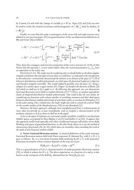
10 P. D. TAFTI AND M. UNSER
by Lemma 2.4 and with the change of variable ρ = A T ω. Eqns (2.5) and (2.6) can now
−γ
be used to verify the rotation invariance and homogeneity of (− `∆) (and, by duality, of
−ξ
−γ
(− ´∆) ).
−ξ
Finally, we note that the scalar counterparts of the vector left and right inverses were
defined in our previous paper [51] (as generalizations of the one-dimensional definitions of
Blu and Unser [4]) as follows:
⎡
⎤
∫
(− `∆) −γ : f → (2π) −d e j〈x,ω〉 ‖ω‖ −2γ ⎢
⎣ ˆf (ω) −
∑ f (k) (0)ω k
⎥
d k! ⎦ dω;
|k|≤⌊2γ− d 2 ⌋
⎡
⎤
(2.17)
∫
(− ´∆) −γ : f → (2π) −d ⎢
⎣ ej〈x,ω〉 −
∑ j |k| x k ω k
⎥
d k! ⎦ ‖ω‖−2γ ˆf (ω) dω.
|k|≤⌊2γ− d 2 ⌋
They share the conjugacy and inversion properties of the vector inverses (cf. (2.10), (2.16)).
Notice that the operand, f , is now scalar-valued. Also, the vectorial parameters ξ irr ,ξ sol have
no equivalent in the scalar case.
DIGRESSION 2.6. The reader may be wondering why we should bother at all about singular
integrals and distinct left and right inverses when we could have—as indicated in the introduction
to this subsection—conveniently characterized the solution as an element of the space ( d ) ′ /Π of
Schwartz distributions modulo polynomials, on which space the fractional Laplacian is bijective
and therefore uniquely invertible. This would indeed be possible, since the space d , being a
0
subspace of a nuclear space, is again nuclear [41, Chapter 5]; therefore the theorems of Minlos [26,
36] which we shall use in §3.1 apply to it. By following this approach, one can characterize
fractional Brownian vector fields as random elements of ( d ) ′ /Π (i.e. as random equivalence
classes of tempered distributions modulo polynomials). One could in fact do even better, by
considering test functions with a finite number of vanishing moments and their dual spaces
(Schwartz distributions modulo polynomials of some finite order), as was done by Dobrushin [11]
in the scalar setting. (On a related note, the reader might also wish to consult the work of Vedel
on the wavelet analysis of the Mumford process [59]; see also Bourdaud [5].)
However, the latter approach—although more straightforward from a technical point of
view—does not provide us, at least immediately, with as complete a characterization of the
stochastic solutions to (2.2) as those we shall see in the sequel.
As far as the spaces of solutions are concerned, another possibility would be to use fractional
Sobolev spaces, as proposed by Ruiz-Medina & al.[45] and Kelbert & al.[23]. It appears that
this approach would work especially well when considering Gaussian self-similar vector fields.
Working with spaces of generalized functions, on the other hand, allows us to use the method of
characteristic functionals [26, 36, 43], which shows its versatility when extending the work to
the study of non-Gaussian random models.
3. Vector fractional Brownian motion. A classical definition of the scalar isotropic
fractional Brownian motion field with Hurst exponent H (denoted B H , with 0 < H < 1)
goes as follows: B H is a zero-mean Gaussian field satisfying B H (0) = 0, with stationary
(Gaussian) increments whose variance depends on the step size as per
E{|B H (x) − B H (y)| 2 } = 2α‖x − y‖ 2H . (3.1)
This is a generalization of Lévy’s characterization of multi-parameter Brownian motion
[30], to which it reduces for H = 1 . The above expectation, as a function of x and y, is also
2
known as the variogram of the field B H (denoted here by Vario[B H ](x, y)).