3. Basic probability concepts

proportion of that outcome that we observe in a sample of observations. The long-run relative
frequency is the proportion that we observe as the sample becomes very large. In most
circumstances, as the sample size increases toward infinity, the relative frequency of the outcome
in the sample will converge on its true value in the population. After estimating the long-run
relative frequency, we then turn the situation around and interpret the frequency as the
probability of observing the outcome of interest by sampling a single observation from the
population.
Say that we want to estimate the allele frequencies of individuals for the MN blood group in
a particular human population. The three possible genotypes are MM, MN, and NN. We could
sample a number of individuals (the more, the better for this purpose, as long as the sample is
representative of the population) and determine the genotype of each. From these we could in
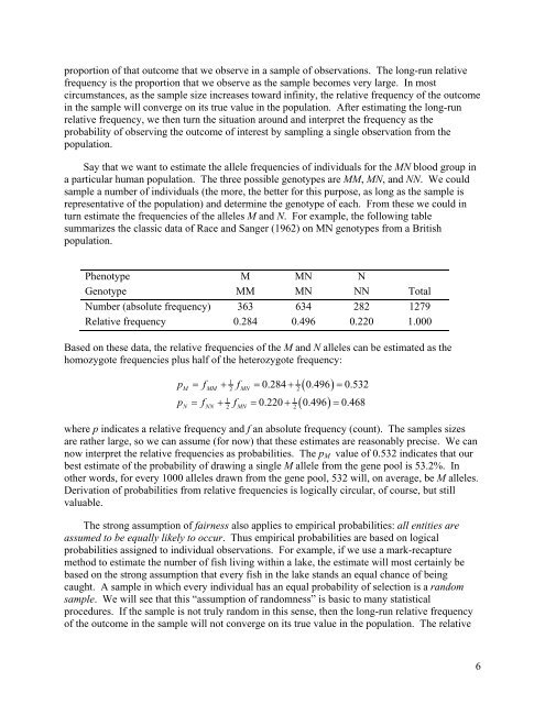
turn estimate the frequencies of the alleles M and N. For example, the following table
summarizes the classic data of Race and Sanger (1962) on MN genotypes from a British
population.
Phenotype M MN N
Genotype MM MN NN Total
Number (absolute frequency) 363 634 282 1279
Relative frequency 0.284 0.496 0.220 1.000
Based on these data, the relative frequencies of the M and N alleles can be estimated as the
homozygote frequencies plus half of the heterozygote frequency:
1 1
M MM 2 MN
2
1 1
N NN 2 MN
2
( )
( )
p = f + f = 0.284 + 0.496 = 0.532
p = f + f = 0.220 + 0.496 = 0.468
where p indicates a relative frequency and f an absolute frequency (count). The samples sizes
are rather large, so we can assume (for now) that these estimates are reasonably precise. We can
now interpret the relative frequencies as probabilities. The p M value of 0.532 indicates that our
best estimate of the probability of drawing a single M allele from the gene pool is 53.2%. In
other words, for every 1000 alleles drawn from the gene pool, 532 will, on average, be M alleles.
Derivation of probabilities from relative frequencies is logically circular, of course, but still
valuable.
The strong assumption of fairness also applies to empirical probabilities: all entities are
assumed to be equally likely to occur. Thus empirical probabilities are based on logical
probabilities assigned to individual observations. For example, if we use a mark-recapture
method to estimate the number of fish living within a lake, the estimate will most certainly be
based on the strong assumption that every fish in the lake stands an equal chance of being
caught. A sample in which every individual has an equal probability of selection is a random
sample. We will see that this “assumption of randomness” is basic to many statistical
procedures. If the sample is not truly random in this sense, then the long-run relative frequency
of the outcome in the sample will not converge on its true value in the population. The relative
6