Math 4330 Sec. 1, Matlab Assignment # 1, March 24, 2006 Name 1 ...

Math 4330 Sec. 1, Matlab Assignment # 1,
March 24, 2006 Name
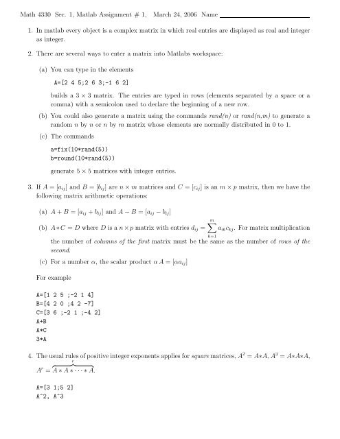
1. In matlab every object is a complex matrix in which real entries are displayed as real and integer
as integer.
2. There are several ways to enter a matrix into Matlabs workspace:
(a) You can type in the elements
A=[2 4 5;2 6 3;-1 6 2]
builds a 3 × 3 matrix. The entries are typed in rows (elements separated by a space or a
comma) with a semicolon used to declare the beginning of a new row.
(b) You could also generate a matrix using the commands rand(n) or rand(n,m) to generate a
random n by n or n by m matrix whose elements are normally distributed in 0 to 1.
(c) The commands
a=fix(10*rand(5))
b=round(10*rand(5))
generate 5 × 5 matrices with integer entries.
3. If A = [a ij ] and B = [b ij ] are n × m matrices and C = [c ij ] is an m × p matrix, then we have the
following matrix arithmetic operations:
(a) A + B = [a ij + b ij ] and A − B = [a ij − b ij ]
(b) A ∗C = D where D is a n ×p matrix with entries d ij =
m∑
a ik c kj . For matrix multiplication
the number of columns of the first matrix must be the same as the number of rows of the
second.
(c) For a number α, the scalar product α A = [αa ij ]
For example
A=[1 2 5 ;-2 1 4]
B=[4 2 0 ;4 2 -7]
C=[3 6 ;-2 1 ;-4 2]
A+B
A*C
3*A
4. The usual rules of positive integer exponents applies for square matrices, A 2 = A∗A, A 3 = A∗A∗A,
r
{ }} {
A r = A ∗ A ∗ · · · ∗ A.
A=[3 1;5 2]
A^2, A^3
k=1

5. In general, division of matrices makes no sense. But for nonsingular square matrices is it is
possible to make an interpretation of matrix division. If A is nonsingular, then it has an inverse,
i.e., a matrix A −1 satisfying A ∗ A −1 = A −1 ∗ A = I where I is the identity matrix with ones on
the main diagonal and zeros elsewhere. The identity matrix plays the same role as the number 1
does for multiplication A ∗I = I ∗A = A. In Matlab the identity matrix is given by eye(n) where
n is an integer. If A is nonsingular, then the inverse in matlab is given by inv(A) or A^(-1).
In this case we can think of division as B ∗ A −1 just as we do with numbers bdiva = b ∗ a −1 for
numbers with a ≠ 0.
6. More generally, in this case, you can compute C=A^(-r).
A=[3 1;5 2]
A^(-1), inv(A)
A*A^(-1)
A=[3 1;5 2]
C=A^(-2)
C*A^2
7. A matrix has an inverse if and only if its determinant is not zero. Recall the determinant for
a square matrix is a number. You can find the definition of the number in most college algebra
books. In Matlab it is easy to compute determinants using the command det.
A=[3 1;5 2]
d=det(A)
8. Recall for a 2 × 2 matrix
[ ]
a11 a
det 12
= a
a 21 a 11 a 22 − a 12 a 21 .
22
9. The problem of determining when a square matrix has an inverse is not easy to answer. The answer
is that precisely the nonsingular matrices have inverses. There are several other characterizations
of nonsingular given below. We will consider these properties with two examples
A=[3 1;5 2]
B=[3 1;6 2]
A matrix A is nonsingular if and only if any one of the following hold:
(a) det A ≠ 0
det(A)
det(B)
(b) The row reduced echelon form of A is the identity
rref(A)
rref(B)

(c) A has an inverse
inv(A)
inv(B)
(d) The only solution of the equation Ax = 0 is x = 0, i.e., the null space is the zero vector.
The Matlab command “null” computes a basis for the null space. Note It does not list the
zero vector.
null(A)
null(B)
(e) The matrix A has full rank. If A is n × n then the rank of A is n.
rank(A)
rank(B)
10. Since we can do powers, scalar products and sums of matrices we can consider matrix polynomials.
Here is an example. Suppose A is an n ×n matrix, c is a (m+1) component row vector, then the
matrix polynomial expression f = c(m + 1) ∗ A m + c(m) ∗ A m−1 + · · · + c(2) ∗ A + c(1) ∗ eye(n).
11. Here is an example
A=[3 1;5 2]
c=[-3 2 -1 5]
f=c(4)*A^3+c(3)*A^2+c(2)*A+c(1)*eye(2)
g=A*(A*(c(4)*A+c(3)*eye(2))+c(2)*eye(2)) +c(1)*eye(2)
%Horner’s method or synthetic division
12. Recall that a system of n linear equations in n unknowns has the form
⎧
a 11 x 1 + a 12 x 2 + · · ·a 1n x n = b 1
⎪⎨ a 21 x 1 + a 22 x 2 + · · ·a 2n x n = b 2
which can also be written in matrix form as
⎪⎩
.
a n1 x 1 + a n2 x 2 + · · ·a nn x n = b n
Ax = b
where
⎡
⎤ ⎡ ⎤ ⎡ ⎤
a 11 a 12 · · · a 1n x 1 b 1
a 21 a 22 · · · a 2n
A = ⎢
⎣
.
. . ..
⎥ . ⎦ , x = x 2
⎢ ⎥
⎣ . ⎦ , b = b 2
⎢ ⎥
⎣ . ⎦ .
a n1 a n2 · · · a nn x n b n
13. A system of equations in this form can be solved in Matlab several different ways. One way is to
use the “backslash” syntax x = A\b.

A=[3 1;5 2]
b=[2;-9]
x=A\b
A*x-b
% setup A
% setup b
% solve Ax=b
% check the result
14. This system can also be solved by writing the augmented matrix [A b] and computing the row
reduced echleon form. The last column is the solution.
A=[3 1;5 2]
b=[2;-9]
C=[A b]
rref(C)
% setup A
% setup b
% setup augmented matrix
% compute row reduced echleon form
15. We now show how difficult solving a system of equations accurately can be. We do this using the
Hilbert matrix.
For each positive integer n the n × n Hilbert matrix is
⎡
1
1
2
H n =
1
3
.
⎢
⎣1
n
1 1 1
⎤
· · ·
2 3 n
1 1 1
· · ·
3 4 (n + 1)
1 1 1
· · ·
4 5 (n + 2)
.
. .. . .. . .. .
⎥
1 1 1 ⎦
· · ·
(n + 1) (n + 2) (2n − 1)
Let us consider a problem where we start with an answer x. Then we set b = H n x and finally try
to solve for x. Thus we set ⎡ ⎤
1
1
x =
1
, b = H n x,
⎢ ⎥
⎣.
⎦
1
We are also interested in the effect of slightly perturbing the values in b. We would guess that
this would result in a very small change in the values of x - but this is not the case.
⎡ ⎤
ǫ 1
ǫ 2
b ǫ = b +
ǫ 3
, |ǫ j | ≤ 10 −8 .
⎢ ⎥
⎣ . ⎦
ǫ n

On the left we solve the resulting system H n x = b. Notice that as N increases the errors get
larger. On the right we have added very small perturbations (less than 10 −8 ) to the right hand
side vector b. Notice what a dramatic effect in the column error which gives the deviation from
the values of x with all ones.
N error cond(H n )
5.000000 0.000000 5 × 10 5
6.000000 0.000000 1 × 10 7
7.000000 0.000000 5 × 10 8
8.000000 0.000000 2 × 10 10
9.000000 0.000005 5 × 10 11
10.000000 0.000259 2 × 10 13
11.000000 0.015063 5 × 10 14
12.000000 0.236949 2 × 10 16
N error b cond(H n )
5.000000 0.000580 5 × 10 5
6.000000 0.024407 1 × 10 7
7.000000 0.197698 5 × 10 8
8.000000 22.485693 2 × 10 10
9.000000 868.368857 5 × 10 11
10.000000 31600.401054 2 × 10 13
11.000000 697526.222439 5 × 10 14
12.000000 4766960.006120 2 × 10 16
Hilbert exact
Hilbert perturbed
In Matlab the above calculations could be carried out as follows:
n=10;
A=hilb(N);
x=ones(N,1);
b=A*x;
x_approx=A\b;
error =norm(x-x_approx,inf);
c=cond(A);
be=b+10^(-8)*rand(N,1);
x_approx_b=A\be;
error_b=norm(x-x_approx_b,inf);

1. Enter the matrices
and carry out the following:
A =
ASSIGNMENT 1
[ ] 2 4
, B =
1 3
(a) Verify that (A + B) + C = A + (B + C)
[ ] −2 1
, C =
0 4
[ ] 3 1
2 1
(A + B) + C = A + (B + C) =
(b) Verify that (AB)C = A(BC)
(AB)C = A(BC) =
(c) Decide whether AB is equal to BA
AB = BA =
(d) Find (A + B) 2 , (A 2 + 2AB + B 2 ) and (A 2 + AB + BA + B 2 )
(A + B) 2 = (A 2 + 2AB + B 2 ) =
(e) Find A 2 − B 2 , (A − B)(A + B)
A 2 − B 2 = (A − B)(A + B) =
2. Enter
and do the following:
A =
[ ] 1/2 1/2
, B =
1/2 1/2
[ 1/2
] −1/2
−1/2 1/2
(a) Compute
A 2 = , A 3 = , etc.
Can you say what A n will be Explain why this is true.
(b) Compute B 2 =
, Can you explain why this is true. What does
this tell you about matrix multiplication that is different from squaring numbers

(c) Find AB = and BA = . What do
you learn from this that is not true for multiplication of numbers (hint: if a and b are real
numbers and ab = 0, then a = 0 or b = 0).
3. Find the inverse of the matrices (if they exist) and check that the result is correct by multiplying
the matrix times its inverse.
[ ]
−1 1
(a) A = , A
1 0
−1 = ,
(b) B =
[ ] 2 5
, B
1 3
−1 = ,
⎡ ⎤
2 0 5
(c) C = ⎣0 3 0⎦, C −1 = ,
1 0 3
⎡ ⎤
−1 −3 −3
(d) D = ⎣ 2 6 1 ⎦, D −1 = ,
3 8 3
[ ]
1 −1
4. Consider the A δ = depending on a parameter δ. The determinant of A
1 −1 + δ
δ is δ so when
δ is small it is clear that the close to having a zero eigenvalue. This does not necessarily mean
the matrix has a large condition number but it raises a red flag. Using Maple I compute the
condition number using the command ConditionNumber(A_d); to get
(∣ ) ∣∣∣ −1 + δ
max
δ ∣ + (|δ|)−1 , 2 (|δ|) −1 max (2, 1 + |−1 + δ|)
Notice here is an example where Maple is preferably since I want the answer in terms of δ.
[
1
Set x = and set b
1]
δ = A d x. We consider δ = 10 −1 and δ = 10 −5 .
(a) For each δ find the eigenvalues and condition numbers of A δ .
(b) For each δ solve A δ x δ = b.
(c) Consider the error obtained between x and x δ .
Now let us perturb the right hand side a little bit.
,
,
,

(a) For each δ (above) set b_e= 10^(-4)*rand(2,1); then solve A δ x δ,ǫ = b e .
(b) Consider the error obtained between x and x δǫ .
,
(c) Repeat parts (a) and (b) above withb_e= 10^(-5)*rand(2,1);
,
5. Given the matrices
solve the matrix equations:
(a) AX + B = C,
A =
[ ]
5 3
, B =
3 2
[ ]
6 2
, C =
2 4
[ ]
4 −2
,
−6 3
(b) AX + B = X,
(c) XA + B = C,
(d) XA + C = X.
6. Let A = round(10 ∗ rand(6)). Change the sixth column as follows. Set
B=A’
% (take the transpose of $A$)
now type
A(:,6)=-sum(B(1:5,:))’
(a) Explain what this last command does

(b) Compute det(A)
(c) Compute rref(A)
(d) Compute rank(A)
7. Explain why A is singular
8. Let A = round(10 ∗ rand(5)) and B = round(10 ∗ rand(5)). Compare the following pairs of
numbers.
(a) det(A) and det(A ′ ).
(b) det(A + B) and det(A) + det(B).
(c) det(AB) and det(A) det(B).
(d) det(A −1 ) and 1/ det(A).
9. Look at help on magic and then compute det(magic(n)) for n = 3, 4, 5, · · · , 10. What seems to
be happening Check n = 24 and 25 to see if the patterns still holds. By pattern I mean try to
describe in words what seems to be happening to these determinants.