6 Variational Methods

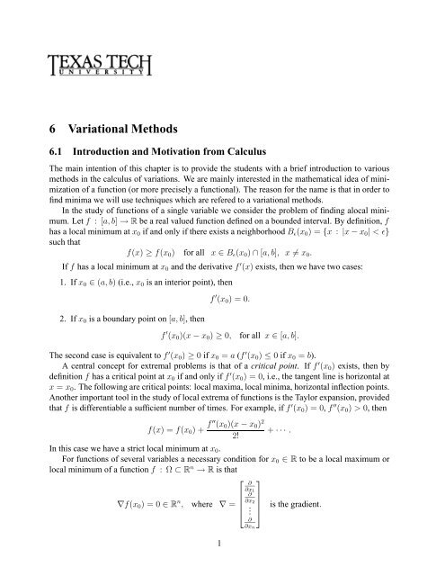
6 Variational Methods6.1 Introduction and Motivation from CalculusThe main intention of this chapter is to provide the students with a brief introduction to variousmethods in the calculus of variations. We are mainly interested in the mathematical idea of minimizationof a function (or more precisely a functional). The reason for the name is that in order tofind minima we will use techniques which are refered to a variational methods.In the study of functions of a single variable we consider the problem of finding alocal minimum.Let f :[a, b] → R be a real valued function defined on a bounded interval. By definition, fhas a local minimum at x 0 if and only if there exists a neighborhood B ɛ (x 0 )={x : |x − x 0 | 0, thenf(x) =f(x 0 )+ f ′′ (x 0 )(x − x 0 ) 2+ ··· .2!In this case we have a strict local minimum at x 0 .For functions of several variables a necessary condition for x 0 ∈ R to be a local maximum orlocal minimum of a function f :Ω⊂ R n → R is that⎡∇f(x 0 )=0∈ R n , where ∇ = ⎢⎣1⎤∂∂x 1∂∂x 2⎥. ⎦∂∂x nis the gradient.

Geometrically, f(x 0 ) is the largest value taken on by f(x) (near x 0 , if for any y ≠0and α ≠0(small enough) we have f(x 0 ) >f(x 0 + αy). Now using taylor’s theorem we havef(x 0 + αy) =f(x 0 )+α∇f(x 0 ) · y + α 2 terms bounded by a constant.Now for small α,if∇f(x 0 ) ≠0, there must be a direction y for which ∇f(x 0 ) · y ≠0. But then achange of signs of α would change the sign of f(x 0 ) − f(x 0 + αy) which is impossible. Thereforewe must have ∇f(x 0 )=0.The main problem in the calculus of variations is to minimize (or maximize) not functions butfunctionals. For example, suppose we have a function F (x, y, z) and we wish to find a functiony(x) which minimizesJ(y) =∫ 10F (x, y(x),y ′ (x)) dx (6.1.1)over the set of C 1 functions, i.e., y ∈ C 1 [0, 1] with y(0) = y 0 and y(1) = y 1 . The class offunctions, C 1 [0, 1] in this case, is called the class of admissible functions for this problem. Supposenow that ỹ ∈ C 1 [0, 1] minimizes J and η(x) is any admissible function with η(0) = η(1)=0.Forany scalar α,wehave∂J∂α (ỹ + αη)∣ ∣α=0=0.By the chain rule this holds if and only if0= ∂J∂α (ỹ + αη)∣ ∣α=0=+ ∂F=∫ 10∫ 10( ∂F∂y (x, (ỹ + αη), (ỹ′ + αη ′ )) ∣ ∣α=0η∂y (x, (ỹ + αη), ′ (ỹ′ + αη ′ )) ∣ )α=0η ′ dx[ ∂F∂y − d ( )] [ ∂F∂Fηdx+dx ∂y ′]∣ ∣∣∣x=1∂y η . (6.1.2)′Here, to obtain the last equality, we have assumed that it is justified, in the second term, tocarry out an integration by parts. We have then set α =0. Assuming that y(0) = y 0 and y(1) = y 1are prescribed, then we need η(0) = η(1)=0. We obtain0=∫ 10[ ∂F∂y − ddxx=0( ∂F∂y ′ )]η dx.This must hold for all admissible η satisfying η(0) = η(1)=0.At this point we obtain an interesting point in mathematical history. Euler, using dubious rigor,concluded that from the above, we can conclude∂F∂y − d ∂F=0. (6.1.3)dx ∂y ′Realizing that Euler had not carefully justified this step gave an alternative derivation by concludingthat if the above integral vanishes for all admissible η vanishing at the end points then thecoefficient of η must vanish. He did not supply a proof of this though and was in turn criticizedby Euler for this shortcoming. It was all put to rest by Dubois Reymond who proved the followingresult called the Fundamental Lemma of the Calculus of Variations.2

Lemma 6.1. If M ∈ C[a, b] and∫ baM(x)η(x) dx =0for all η ∈ S = {ϕ ∈ C 1 [a, b] :ϕ(0) = ϕ(1)=0}, thenM(x) =0 for all x ∈ [a, b].by contradiction. Suppose there exists an x 0 ∈ (a, b) so that M(x 0 ) ≠0. Then we can, withoutloss of generality, assume that M(x 0 > 0. Since M ∈ C[a, b], there exists a B ɛ (x 0 ) ⊂ (a, b) suchthat M(x) > 0 for all x ∈ B ɛ (x 0 ).Let{(x − x 0 − ɛ) 2 (x − x 0 + ɛ) 2 for x ∈ B ɛ (x 0 )η(x) =0 for x ∉ B ɛ (x 0 ).With this choice of admissible η we have∫ baM(x)η(x) dx =∫ (x−x0 +ɛ)(x−x 0 −ɛ)M(x)(x − x 0 − ɛ) 2 (x − x 0 + ɛ) 2 dx > 0,which contradicts our hypothesis. Thus we have M(x) =0for all x ∈ (a, b). By continuity wealso must have M(a) =M(b) =0.Remark 6.1.1. The equation (6.1.3) is called the Euler-Lagrange equation.2. A solution of the Euler-Lagrange equation is called an extremal.3. An extremal that satisfies the end conditions is called a stationary function. Such a functionstill may or may not be a maximum or minimum for j.4. We note that in the derivatives ∂F∂yand∂F∂y ′ we treat x, y and y ′ as independent variables.5. Since ∂F is, in general, a function of x explicitly and also implicitly through y and y ′ , the∂y ′second term in (6.1.3) can be written in expanded form as∂∂x( ∂F∂y ′ )+ ∂ ∂yThus the Euler-Lagrange equation can be eritten as( ∂F∂y ′ ) dydx + ∂∂y ′ ( ∂F∂y ′ ) dy′dx .d 2 yF y ′ y ′ dx + F dy2 y ′ ydx +(F y ′ x − F y )=0. (6.1.4)6. The equation is of second order in y unless F y ′ y ′ = ∂2 F∂y ′ 2=0so that, in general, there aretwo constants of integration available to satisfy the two end conditions.3

7. The equation (6.1.4) is equivalent to[1 dy ′ dx(F − ∂F∂y ′ dydx8. There are some special cases of (6.1.3) and (6.1.5):(a) From (6.1.5) we see that if F does not depend explicitly on x, i.e.,J =∫ ba)− ∂F ]=0 (6.1.5)∂xF (y, y ′ ) dxthenF − y − ddx F y ′ = F y − F y ′ yy ′ − F y ′ y ′y′′ .Multiplying by y ′ we haveF y y ′ − F y ′ y(y ′ ) 2 − F y ′ y ′y′ y ′′ = ddx (F − y′ F y ′) .Thus we have∂F∂F=0 ⇒ F − = c.∂x ∂y ′(b) From (6.1.5) we see that if F does not depend explicitly on y, i.e.,J =∫ baF (x, y ′ ) dxthen In this case Euler’s equation becomesddx F y ′ =0which gives F y ′ =0where F does not contain y. This is a first order Euler equationand solving for y ′ we havey ′ = f(x, c)which can be solved by quadrature. Thus∂F∂y=0 ⇒∂F∂y ′ = c.(c) From (6.1.5) we see that if F does not depend explicitly on y ′ , i.e.,J =∫ baF (x, y) dxthen Euler’s equation becomesF y (x, y) =0and hence it is not a differential equation but simply an equation whose solution consistsof one or more curves.4

9. In many problems the functional J has the special formJ =∫ baf(x, y) √ 1+(y ′ ) 2 dx,representing the integral of a function f(x, y) with respect to arclength s (so ds = √ 1+(y ′ ) 2 dx).In this case Euler’s equation can be transformed into∂F∂y − d ∂F= fdx ∂y ′ ( x, y) √ []1+(y ′ ) 2 − dy ′f(x, y) √dx 1+(y′ ) 2Thus we obtain√ y ′= f y 1+(y′ ) 2 − f x √1+(y′ ) − f (y ′ ) 22 y √1+(y′ ) − f y ′′2 (1 + (y ′ ) 2 ) 3/2=)1√(f y − f x y ′ y ′′− f.1+(y′ ) 2 (1 + (y ′ ) 2 )y ′′f y − f x y ′ − f(1 + (y ′ ) 2 )(6.1.6)6.1.1 Simple ExamplesLet us begin with a simple exampleExample 6.1. Find the minimal surface of revolution passing through two given points (x 1 ,y 1 ),(x 2 ,y 2 ) in the plane. This leads to minimizing the integralJ =2π∫ x2x 1y(1 + (y ′ ) 2 ) 1/2 dx. (6.1.7)The surface area ∆S of a small surface of revolution formed by revolving the curve y = y(x)from x = x 1 to x = x 2 about the x-axis approximately equals the circumference 2yπ times thearclength of the curve from y(x) to y(x +∆x), denoted by ∆s:∆S =2πy∆s.5

Now recall that infinitesimal arc length is given by√∆s ≈ √ (∆x) 2 +(∆y) 2 =1+( ) 2 ∆y∆x.∆xThus we obtain∫ x2S =(2π) y(x) √ 1+(y ′ (x)) 2 dx.x 1Thus we haveF (x, y, y ′ )=2πy √ 1+(y ′ ) 2and the Euler equation (6.1.3) becomes[]d yy ′− (1+(y ′ ) 2 ) 1/2 =0.dx (1+(y ′ ) 2 ) 1/2If we use (6.1.5) then we getTo solve this equation we letyy ′′ − (y ′ ) 2 − 1=0.p = y ′ so that y ′′ = dpdx = dp dydy dx = pdp dyand this givespy dpdy = p2 +1.This equation is separable, and is integrated as followspdpp 2 +1 = dyy⇒1 2 ln(p2 + 1) = ln(y)+C.Exponentiating both sides we getSolving for dy/dx we get(y = α 1+( ) ) 2 1/2dy.dxdydx = ( y2α − 1 ) 1/2,6

and separating variables again, we getdy√(y/α)2 − 1 = dx.Now let y = α cosh(t) so that (y/α) 2 − 1 = cosh 2 (t) − 1 = sinh 2 (t), and dy = α sinh(t) dt.∫ ∫∫sinh(t) dtdx = α = α dt = αt + csinh(t)(x − b)so x = αt + β which implies t =α( ) x − βy = α cosh .αThus the minimal surface, if it exists, is a cantenary. It remains to be seen whether the arbitraryconstants α and β can be chosen that the curve passes through the points (x 1 ,y 1 ) and (x 2 ,y 2 ).This can be done for any two points in the upper half plane. In general, the determine of the twoconstants involves the solution os a transcendental equation which possess two, one or no solutions,depending on y(x 1 ) and y(x 2 ).Let us fix the initial point (x 1 ,y 1 ) to be (0, 1). We show that there are point which cannot bereached to solve the extremal problem, i.e., the boundary value problem has no soultion.First since we need y(0)=1we haveLet us denote λ = β/α so we have( β1=α cosh( , or α =α)1cosh(β/α) .cosh(x cosh(λ) − λ)y = y(x, λ) = .cosh(λ)Since y ′ = sinh(x cosh(λ) − λ) we have y ′ (0) = − sinh(λ). Thus as λ varies over all realnumbers we get all possible slopes. Now we try to find λ so that the curve passes through thesecond point which we now denote as (b, y b ). So we need to solve the equationcosh(b cosh(λ) − λ)y(b, λ) = = y b .cosh(λ)We now show that (b, y b ) can be chosen so that this equation has no solution.First note thatcosh(t) = 1 2 (et + e −t ) ≥|t| for all t.hencecosh(b cosh(λ) − λ)cosh(λ)≥(b cosh(λ) − λ)∣ cosh(λ)=∣ b − λcosh(λ) ∣7≥|b|−|λ|cosh(λ)∣

it is easy to see thatmaxλλ∣cosh(λ)∣ = |λ| 0cosh(λ 0 )where λ 0 is the positive root of the equationThus we haveand finallycosh(λ 0 ) − λ 0 sinh(λ 0 )=0.|b|−y(b, λ) ≥|b|−λcosh(λ) ≥|b|− 1sinh(λ 0 ) ,1, for all λ.sinh(λ 0 )So if b is chosen so that1|b|−sinh(λ 0 ) = B>0and y b is then chosen so that y b 0) and the final point is y(b) =0. We assume thatthe speed of travel in the particular medium is given at each point by c(x, y). Thendsc(x, y)dtwhere ds is incrmental arclength. Then the total time of travel is∫ b√1+(y′ )T =2 dx.0 c(x, y)Since the particle is at rest at height y 0 , and since the potential plus kenetic energies is a constant,the speed at height y is c = √ 2g(y 0 − y) where g is the gravitational constant.Put another way, if s represents distance on the curve y = y(x) measured from (0,y 0 ), thendsdt = vwhere t represents time and v is the velocity of the particle. Since the motion, by assumption, isfrictionless with initial velocity v 0 =0and is influenced only by gravity, the principle of conservationof energy implies12 mv2 = mg(y 0 − y)8

where y is the vertical distance, and m is the mass of the particle.This impliesv = √ 2gy.Hencedsdt = √ 2g(y 0 − y) or dt =√ds√2g(y0 − y) = 1+(y′ ) 2 dx√2g(y0 − y) .Therefore the time T that the particle takes to get from (0,y 0 ) to (b, 0) along the curve y = y(x) isgiven byT = √ 1 ∫ b√1+(y′ ) 2 dx√ .2g 0 (y0 − y)The problem is to find y(x) to minimize T .In our notation we have√F (x, y, y ′ 1+(y)=′ ) 2(y 0 − y) .Note that F does not depend on x explicitly, so the Euler equation has the formy ′ ∂F∂y ′ − F = c 0or ((y0 − y)(1+(y ′ ) 2 ) ) 1/2= c0 .From this we obtain a first order ODE(dy c2dx = − 0 − (y 0 − y)(y 0 − y)with c 0 an arbitrary constant of integration. To solve this equation we introduce a parametricsubstitutiony = y 0 + c 2 0(cos(t) − 1)/2.It follows thatand) 1/2y − y 0 = c 2 0(cos(t) − 1)/2( )dy c2dx = − 0 + c 2 1/2 ( )0(cos(t) − 1)/2c2 1/2= − 0 (1 + (cos(t) − 1)/2)c 2 0(1 − cos(t))/2c 2 0(1 − cos(t))/2( ) 1/2 ( ) 1/2 ( ) (cos(t)+1)/2(1 + cos(t))(1 − cos(t) 2 1/2)= −= −= −(1 − cos(t))/2(1 − cos(t))(1 − cos(t)) 2( ) sin 2 1/2 ( )(t)sin(t)= −= −(1 − cos(t)) 2 (1 − cos(t))9

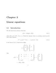
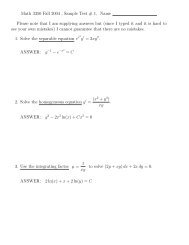
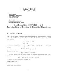
Thus we obtainand sincewe havedxdtFrom this we obtain(1 − cos(t)) dy=− sin(t) dtdydx =−sin(t)(1 − cos(t))dydt = c2 0(− sin(xt))2(1 − cos(t)) c 2=0(− sin(t))− sin(t) 2= c2 0(1 − cos(t)).2x = 1 2 c2 0(t − sin(t)), y = y 0 + c 2 0(cos(t) − 1)/2. (6.1.8)The constant c 0 must be chosen so that y =0when x = b. Set x = b and y =0in in (6.1.8),then solve each of the equations for c 2 0c 2 0 =2bt − sin(t) , c2 0 =Next we equate these expressions, eliminating c 2 0, to obtainorh(t) ≡bt − sin(t) = y 01 − cos(t)( ) 1 − cos(t)=t − sin(t)2y 01 − cos(t) .( y0).bAs t varies from 0 to +∞, the left hand side of this last expression, i.e., h(t), varies from ∞ to0. So for any positive values y 0 and b we can find a value T 0 so that( y0)h(T 0 )= .bFrom this we can determine c 0 by√2y 0c 0 =1 − cos(T 0 ) .In this way we can obtain the solution which describes a cycloid curve parameterized by{(x(t),y(t)):0≤ t ≤ T 0 }.The following numerical example corresponds to y 0 =2and b =1.10

2y 0= 2 b = 11.5y10.500 0.2 0.4 0.6 0.8 1xWe now give an example to show that the extremal function may not be C 1 .Example 6.3. Consider the problem of minimizingsubject to the boundary conditionsJ =∫ 1−1y 2 (1 − (y ′ ) 2 ) dx (6.1.9)y(−1)=0,y(1)=1.It is obvious that y =0and y = x both give minimal values for J, namely J =0. But it turnsout that neither of these satisfies the end conditions. In order to obtain a solution that satisifiesthese conditions we must build a piecewise smooth solution. The function{0 for − 1 ≤ x

then at all points x = c where y 0 ′ is discontinuous (with a jump discontinuity), the Weierstrass-Erdmann Corner Conditions∣f y ′∣x=c −= f y ′and∣x=c +must be satisfied.(y ′ f y ′ − f) ∣ ∣x=c −=(y ′ f y ′ − f) ∣ ∣x=c +Functionals of Several Unknown Functions:Suppose we want to find the extremal of a functional of several unknown functionsJ =∫ baF (x, y 1 ,y ′ 1,y 2 ,y ′ 2, ··· ,y k ,y ′ k) dx. (6.1.10)We proceed to derive Euler equations by introducing functions η j and assume that y ∗ j are extremalfunctions. Then we introduce the admissible functions y j = y ∗ j + α j η j , j =1, 2, ··· ,k where α jare scalar. We require that∣∂J ∣∣∣αj=0, j =1, 2, ··· ,k, for all functions η j .∂α j =0This gives us the system of k Euler-Lagrange equations∂F− d∂y j dx∂F∂y ′ j=0, j =1, 2, ··· ,k.Functionals with Higher Order Derivatives:Suppose we wish to minimize (or maximize) a functional involving higher order derivatives.Consider, for example,J =∫ bHere we suppose that the values ofaF(x, y, dy)dx , d2 ydx ··· , dk ydx. (6.1.11)2 dx ky, dydx , d2 ydx 2 ··· , d(k−1) ydx (k−1)are specified at x = a and x = b. Again we introduce admissible functionsy = y ∗ + αη,12

where y ∗ is an extremal and η satisifesη(a) =η(b) = dη (a) =dηdx dx (b) =···= d(k−1) ηdx (a) η(k−1) =d(k−1) (b) =0.dx(k−1)Repeating the usual procedure we obtainF y − ddx F y ′ + d2dx F dk2 y ′′ + ···+(−1)kdx F k y (k) =0.Natural Boundary Conditions:One other important consideration is that for some problems we are not given fixed endpointconditions. In this case the procedure changes some. Suppose we want to minimumize (or maximize)∫ 1J = F (x, y, y ′ ) dx0but without specifying values of y at x = 0 or x = 1. In this case the difference, αη of theminimimum y and the varied function y + αη need not be zero at the ends (since no end conditionsare required of y). However, the integral term in (6.1.2) must still vanish, since among all possibleadmissible functions η are those which vanish at the end points and we can apply Lemma 6.1 toobtain the Euler equation. Now since the fisrt term is zero we now find that[ ∂F∂y ′ η ]∣∣∣∣x=1−[ ∂F∂y ′ η ]∣∣∣∣x=0=0for all admissible η, which in turn means for all values of η(0) and η(1) if y is not prescribed ateither end. In this case we have the additional requirements[ ∂F∂y ′ ]∣∣∣∣x=0=0,[ ∂F∂y ′ ]∣∣∣∣x=1=0 (6.1.12)Further, if y(0) is not prescribed then the first identity in (6.1.12) must hold and if y(1) is notprescribed then the second identity in (6.1.12) must hold. The conditions in (6.1.12) are called thenatural boundary conditions.In some cases it may also happen that the integrand F or ∂Fand/or (d/dx)∂F∂y ′ are discontin-∂yuous at one or more points inside the interval (0, 1) but the conditions assumed above are satisifedin each subinterval separated by these points. For example, suppose there is one point of discontinuityx = c. Then the integral (6.1.1) must be expressed as two integrals, one over (0,c − ) and theother over (c + , 1):∂J∂α = ∂∂α( ∫ c −F (x, y + αη, y ′ + αη ′ ) dx +0)F (x, y + αη, y ′ + αη ′ ) dxc +∫ 1(6.1.13)13

We obtain∫ c − ( ∂F0=0 ∂y − d ) ∫∂F1ηdx+dx ∂y ′( [∂F ]∣ ∣∣∣c − [ ]∣ )∂F ∣∣∣1+∂y η −′0∂y η .′c +c + ( ∂F∂y − ddx)∂Fηdx∂y ′If we require that the minimizing function y be continuous on (0, 1) (in particular at x = c),then then we also need all admissible functions y + αη to also be continuous. It follows thatη(c − )=η(c + )=η(c).From this we can write∫ c − ( ∂F0=0 ∂y − d ) ∫∂F1( ∂Fηdx+dx ∂y ′ c ∂y − d )∂Fηdxdx ∂y + ′[ ]∣ [ ]∣ ([ ]∣ [ ]∣ )∂F ∣∣∣1 ∂F ∣∣∣0 ∂F ∣∣∣c ∂F ∣∣∣c+ η(1) − η(0) − − η(c).∂y ′ ∂y ′ ∂y ′ + ∂y ′ −Now since η(0), η(1) and η(c) are arbitrary we can conclude that Euler equation( ∂F∂y − d )∂F=0dx ∂y ′must hold in each subinterval (0,c − ) and (c + , 1). We also see that ∂F must vanish at any endpoint∂y′for which y has not been prescribed. Finally, the natural transition conditions must hold:y(c + )=y(c − ∂F ∂F), lim = limx→c + ∂y ′ x→c − ∂y . (6.1.14)′These conditions require that y be continuous but that y ′ may be discontinuous at x = c.Example 6.4. Consider finding the stationary∫ 1(J = T (y ′ ) 2 − ρω 2 y 2) dx (6.1.15)0where T , ρ, and ω are given constants (or functions of x).The Euler equation becomes(dT dy )+ ρω 2 y =0,dx dxregardless of what is presecribed at the endpoints of the interval.If, for example, T , ρ and ω are positive constants, then the extremals are of the form)y = c 1 cos(αx)+c 2 sin(αx),(α 2 = ρω2 .T14

1. If y(0)=0and y(1) = 1 are prescribed then c 1 =0, and c 2 sin(α) =1which impliesy = sin(αx) for α ≠ π, 2π, ··· .sin(α)2. If y(1)=1is prescribed but y(0) is not prescribed then from[ ]∣ ( ) ∣ ∂F ∣∣∣0 ∂[T (y ′ ) 2 + ρω 2 y 2 ] ∣∣∣x=0==0,∂y ′ ∂y ′we obtainTy ′ (0)=0and hencey = cos(αx) for α ≠ π cos(α)2 , 3π 2 , ··· .3. If neither y(0) or y(1) is prescribed then the conditions requireTy ′ (0) = 0, Ty ′ (1)=0and we otain{0 (α ≠ π, 2π, ···)y =c 1 cos(αx) (α = π, 2π, ···) ,where c 1 is an arbitrary constant.In the exceptional cases above there are no stationary functions. The limiting case α =0mustbe treated as a special case where we replace sin(αx) by sin(αx)/α then pass to the limit.Let us now consider the case in which T and ρ are step functions with constant values onsubintervals (0,c) and (c, 1) with 0

Several Independent Variables:In the case of functions of more than one variable we might encounter an extremal problem ofthe form∫ (J = F x 1 ,x 2 , ··· ,x k ,y, ∂y , ∂y , ··· , ∂y )dx 1 dx 1 ···dx k , (6.1.16)∂x 1 ∂x 2 ∂x kDwhere D is a region in R k . The usual arguments considered in more detail in the 2-dimensionalcase below lead to the following. We assume that η is a function of (x 1 ,x 2 , ··· ,x k ) that vanisheson the boundary of D. We replace y by y + αη and compute the derivative with respect to α toobtain∫D(∂F∂y +k∑j=1)∂F ∂ηdx 1 dx 1 ···dx k =0,∂z j ∂x jwhere z j = ∂y∂x j.To use integration by parts in higher dimensions we recall the divergence theorem which statesTheorem 6.2. For a vector valued function f∫∫div (f) dV =D∂Df · ⃗nds (6.1.17)where dV is volume measure, ds is surface measure, ⃗n is the outward normal vector to the boundaryof D which is denoted by ∂D.With this we have∫ k∑D j=1(∂η ∂F ) ∫ ([ ∂FdV = η , ··· , ∂F ] )· ⃗n ds,∂x j ∂z j ∂D ∂z 1 ∂z kso that (also using the product rule)∫ ( k∑) ∫ ([∂F ∂η∂FdV = η , ··· , ∂F ] ) ∫· ⃗n ds − ηD ∂zj=1 j ∂x j ∂D ∂z 1 ∂z k DNow we impose the boundary condition η =0on ∂D. Thus we conclude∂F∂y −k∑j=1k∑j=1∂∂x j( ∂F∂z j)dV,∂∂x j( ∂F∂z j)=0, z j = ∂y∂x j. (6.1.18)If the function y is not prescribed a priori on ∂D, then we cannot assume that η =0on ∂D.Instead we have∂F· ⃗n =0,∂z jon the part of the boundary ∂D where y is not prescribed.16z j = ∂y∂x j,

Remark 6.2. It is important that we point out that in this whole discussion we have only considerednecessary conditions for an extrema. That is an extrema will satisfy the Euler-lagrangeequation. Recall that from calculus a necessary condition for a mimimum (or maximum) at x = x 0is that f ′ (x 0 )=0but just from this we cannot conclude that x 0 gives a local extrema (for example,it could give a point of inflection). On the other hand the second derivative test (when itis applicable) does give us sufficient conditions for an extrema (f ′′ (x 0 ) > 0 implies that x 0 is aminimum and f ′′ (x 0 ) < 0 implies that x 0 is a maximum). This is called the second derivativetest. In the calculus of variations there is an analogous sufficient condition that comes from theso-called second variation. Actually this second variation is seldom used in practice. Generallyother methods are used to verify that a stationary value is actually an extrema. These argumentsare generally somewhat more complicated and won’t be considered here.Example 6.5 (Plateau’s Problem). As an example let us consider the problem of finding a surfacepassing through a given closed curve C in space and having minimum surface area bounded by C.If we assume that the surface can be represented as a function z = z(x, y) then the area to beminimized is given by the integral∫∫J =R( )1+z2x + zy2 1/2dxdy (6.1.19)where R, is the region in the xy plane bounded by the projection C 0 of C onto the xy plane andwhere z is given along C 0 , i.e., if (x(t),y(t)) is a parameterization of C 0 , then the values of z on Care prescribed in terms of a further parameteriztion of C given by z(x(t),y(t)) = h(t) where weare given h. WefindF (x, y, z, z x ,z y )= ( )1+zx 2 + zy2 1/2and the Euler equation is[] []∂ z x( )∂x 1+z2x + zy2 1/2+ ∂ z y( )∂y 1+z2x + zy2 1/2=0.After some simplification this can be written asNote this is a partial differential equation.(1 + z 2 y)z xx − 2z x z y z xy +(1+z 2 x)z yy =0.Example 6.6 (Dirichlet Problem). Next we consider an example that arises in a tremendous numberof practical situations – the Dirichlet Problem. In two dimensions we must minimize the functional∫∫D[u] =R( )u2x + u 2 y dxdy (6.1.20)where R, is the region in the xy plane bounded by the projection C 0 of C onto the xy plane andwhere u is given along C 0 :u(x(t),y(t)) = g(t), t ∈ [a, b].17

In this case findF (x, y, u, u x ,u y )=u 2 x + u 2 yand the Euler equation isu xx + u yy =0.This equation is called Laplace’s equation.Problems with Contraints: Lagrange Multipliers:In many problems we not only need to minimize a functional but this must be carried outsubject to some additional constraints. An important method for dealing with problems of thistype is the Method of Lagrange Multipliers. Let us suppose that we want to minimize a functionalJ[y] =∫ 10F (x, y, y ′ ) dx (6.1.21)where y is prescribed at the endpoints by y(0) = y 0 and y(1) = y 1 and y is subject to the extraconstraint thatK =∫ 10G(x, y, y ′ ) dx = l. (6.1.22)We consider a variation of y in the form y + α 1 η 1 + α 2 η 2 where η 1 and η 2 are continuouslydifferentiable and vanish at the endpoints. This we considerJ(α 1 ,α 2 ) ≡ ∫ 1F (x, y + α ⎫0 1η 1 + α 2 η 2 ,y ′ + α 1 η 1 ′ + α 2 η 2) ′ dx ⎬K(α 1 ,α 2 ) ≡ ∫ 1G(x, y + α 0 1η 1 + α 2 η 2 ,y ′ + α 1 η 1 ′ + α 2 η 2) ′ ⎭ ,dxand it must be true that J(α 1 ,α 2 ) takes on a minimum value subject to the constraint K(α 1 ,α 2 )=0when α 1 = α 2 =0. Thus as in multidimensional calculus we want to find a minimum of a functionof (α 1 ,α 2 ) subject to a constraint. One of the most useful tools for solving problems of this typeis the method of Lagrange Multipliers.We consider∂[J(α 1 ,α 2 )+λK(α 1 ,α 2 )] ∣ ∂α α1 =α 2=0, (6.1.23)=0 1∂[J(α 1 ,α 2 )+λK(α 1 ,α 2 )] ∣ ∂α α1 =α 2=0. (6.1.24)=0 2If we carry out the necessary steps and do integration by parts in each of the approriate terms, weend up with the two equations∫ 1[( ∂F∂y − ddx0∫ 10( ∂F∂y ′ ))+ λ( ∂G∂y − d ( ))] ∂Gηdx ∂y ′ 1 dx =0, (6.1.25)[( ∂F∂y − d ( )) ( ∂F ∂G+ λdx ∂y ′ ∂y − d ( ))] ∂Gηdx ∂y ′ 2 dx =0. (6.1.26)18

Generally it can be assumed that the coefficient of λη 2 in (6.1.26) is not identically zero so it canbe assumed that ∫ 1( ∂G0 ∂y − d ( )) ∂Gη 2 dx ≠0.dx ∂y xIn this case we can choose λ so that (6.1.26) is satisfied. Then since η 1 in (6.1.25) is arbitrary itscosefficient in (6.1.25) must vanish. We obtain( )∂d ∂(F + λG) −∂y dx ∂y (F + λG) =0. (6.1.27)′The general solution of this problem will involve the constant parameter λ as well as the twoconstants of integration. This corresponds to the fact that we have two end conditions and oneextra constraint given in (6.1.22).Remark 6.3. In order to maximize (or minimize) an integral∫ b∫aba∫ baFdxsubject to a constraintGdx = l, first write H = F + λG, where λ is a constant, and maximize (or minimize)Hdx subject to no contraint. Carry the Lagrange multiplier λ through the calculation, anddetermine it, together with the constants of integration arising in the solution of Euler’s equation,so that the constraint is satisfied and so that the end conditions are satisfied. a b Gdx= lWhen one of the end conditions (y(0) = y 0 or y(1) = y 1 ) is not imposed then the condition∂H=0must be substituted for it at the end in question.∂y ′Example 6.7. Consider the problem of determining the curve of fixed length l which passesthrough the points (0, 0) and (0, 1) and for which the area between the curve and the x axis isa maximum. We are thus lead to maximize the integralJ[y] =∫ 10ydx (6.1.28)subject to the end constraints y(0)=0and y(1)=0and also subject to the constraintK =∫ 1The corresponding Euler equation for0(1+(y ′ ) 2) 1/2dx = l.H = y + λ ( 1+(y ′ ) 2) 1/2is[]λ d y ′(dx 1+(y′ ) 2) 1/2− 1=0.19

After integraion and simplification(y ′ ) 2 =Solving for y ′ and integrating again we find(x − c 1 ) 2[λ 2 − (x − c 1 ) 2 ] .y = ± [ λ 2 − (x − c 1 ) 2] 1/2+ c2 .Rearranging terms we find (as you would expect)(x − c 1 ) 2 +(y − c 2 ) 2 = λ 2corresponding to arcs of a circle. The constants c 1 , c 2 and λ are to be determined so that the arcpasses through (0, 0), (1, 0) and has length l.Example 6.8 (Sturm-Liouville Problems). The problem of finding the eigenvalues and eigenvectorsof a Sturm-Liouville problem can be formulated as a variational problem. Consider thefunctional∫ 1(J[y] = p(x)(y ′ (x)) 2 + q(x)y(x) 2) dx (6.1.29)subject to a constraint0K[y] =∫ 10ω(x)y(x) 2 dx =1, (6.1.30)where the functions p, q and ω are positive on the interval 0 ≤ x ≤ 1.We propose to minimize (6.1.29) subject to (6.1.30), which using Lagrange multiplyiers isequivalent to minimizingH[y] =J[y]+λK[y].The Euler-Lagrange equation is(p(x)y ′ ) ′ − q(x)y + λω(x)y =0,subject to any set of boundary conditions for which1p(x)y ′ η∣ =0,where η(x) is any admissible function.If y is the minimizer of J subject to K =1, then λ is an eigenvalue with eigenfunction y.For example, if we have specified y(0) = y 0 and y(1) = y 1 , then we need η(0) = η(1)=0.If η is not specified at 0 and 1 then we must have the natrual boundary conditions y ′ (0) = 0 andy ′ (1) = 0. These correspond to Neumann and Dirichlet boundary conditions. For more generalboundary conditions we must replace J with∫ 1(J[y] = p(x)(y ′ (x)) 2 + q(x)y(x) 2) dx + σ(1)p(1)y 2 (1) + σ(0)p(0)y 2 (0) (6.1.31)0020

still subject to (6.1.30). The Euler-Lagrange equation is againbut now the natural boundary conditions are(p(x)y ′ ) ′ − q(x)y + λω(x)y =0,−y ′ (0) + σ(0)y(0)=0,y ′ (1) + σ(1)y(1)=0.The conclusions in Example (6.8) lead to an important point in the history of mathematics.Minimum Principle1. If y renders J[y] minimal subject to the restriction K[y] = 1, then (p(x)y ′ ) ′ − q(x)y +λω(x)y =0and the minimal value J[y] =λ.2. Suppose the first k eigenfunctions y 1 ,y 2 , ··· ,y k of(p(x)y ′ ) ′ − q(x)y + λω(x)y =0 with λ 1 ≤ λ 2 ≤···≤λ k known.Then the (k +1)st eigenpair (y (k+1) ,λ (k+1) isdetermined as the solution of the minimum ofJ[y] minimal subject to the restriction K[y] =1and the k additional constraints∫ 10y(x)y j (x) dx =0,j =1, 2, ··· ,k.Furthermore we haveis the (k +1)st eigenvalue.J[y (k+1) ]=λ (k+1) ≥ λ k ,Assignment Chapter 61. Consider finding a continuously differentiable function y(x) which minimizesJ[y] =∫ 10(1+(y ′ ) 2 ) dx,y(0)=0, y(1)=1.(a) Obtain the relevant Euler equation, and show that the stationary function is y = x.(b) With y(x) =x and the special choice η(x) =x(1 − x), calculateJ(α) =J[y + αη] =∫ 1and verify directly that dJdα (α)∣ ∣α=0=0.0F (x, y(x)+αη(x),y ′ (x)+αη ′ (x)) dx21

(c) By writing y(x) =x + u(x), show that the problem becomesJ =2+∫ 10(u ′ (x)) 2 dx = minimum,where u(0) = u(1) = 0. Use this result to deduce that y(x) = x is the requiredminimum.2. Find extremal curves for J =3. Find extremal curves for J =∫ ba∫ ba(y 2 − (y ′ ) 2 − 2y cos(x)) dx(y ′ ) 2x 3dx4. Find the extrema for J =∫ 21√1+(y′ ) 2dx,xy(1)=0, y(2)=1.5. Find the extrema for J =∫ ba(x − y) 2 dx.6. Find the arc with the shortest distance between the two points (0,a) and (1,b). Here you canassume that the solution can be expressed as a function of one variable y = y(x).7. Find the curve y(x), 0 ≤ x ≤ 1,withy(0) = y(1)=0and fixed arclength 3π/4 that gives amaximum area∫ 1A = y(x) dx.0Note that this is the Example 6.7. Thus this problem amounts to filling in all the details (i.e.,solving the differential equation, finding the constants, etc.) for Example 6.7 with a specificl.∫ 1( 18. Which curve minimizes0 2 (y′ ) 2 + yy ′ + y ′ + y)dx when y(0) and y(1) are notspecified.9. Determine the stationary functions associated with the integralwhere α and β are constants:(a) y(0)=0and y(1)=1,(b) y(0)=0(c) y(1)=1(d) No end conditions.Note any exceptional cases.J =∫ 10((y ′ ) 2 − 2αyy ′ − 2βy ′) dx,22

10. Find the stationary solutions for the variational problem with constraint: Minimizesubject to the constraintReferencesJ[y] =∫ π0(y ′ ) 2 dx, y(0)=0, y(π) =0,∫ π0y 2 dx =1.[1] G.A. Bliss, “Lectures on the Calculus of Variations,” Unmiv. of chicago Press, 1946.[2] G.M. Ewing, “Calculus of Variations with Applications,” Dover, 1985.[3] I.M. Gelfand, S.V, Fomin, “Calculus of Variations,” Prentice Hall, 1963.[4] F.B. Hildebrand, “Methods of Applied mathematics,” Dover, 1992.[5] J. Keener, “Principles of Applied mathematics,” Addison-Wesley, 1988.[6] H. Sagan, “Introduction to the calculus of variations,” Dover, 1992.[7] D.R. Smith, “Variational Methods in Optimization,” Dover, 1998.[8] I. Stakgold, “Green’s Functions and Boundary Value Problems,” Wiley-Interscience, 1979.[9] E. Zeidler, “Nonlinear Functional Analysis and its Applications III: Variantional Methodsand Optimization,” Springer-Verlag, 1985.23