6 Variational Methods

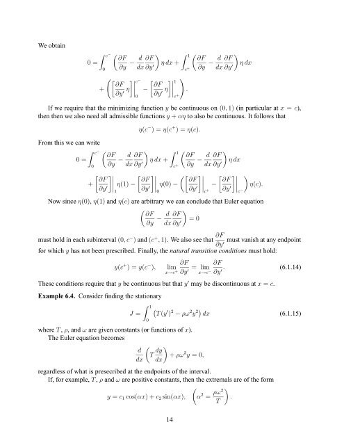
We obtain∫ c − ( ∂F0=0 ∂y − d ) ∫∂F1ηdx+dx ∂y ′( [∂F ]∣ ∣∣∣c − [ ]∣ )∂F ∣∣∣1+∂y η −′0∂y η .′c +c + ( ∂F∂y − ddx)∂Fηdx∂y ′If we require that the minimizing function y be continuous on (0, 1) (in particular at x = c),then then we also need all admissible functions y + αη to also be continuous. It follows thatη(c − )=η(c + )=η(c).From this we can write∫ c − ( ∂F0=0 ∂y − d ) ∫∂F1( ∂Fηdx+dx ∂y ′ c ∂y − d )∂Fηdxdx ∂y + ′[ ]∣ [ ]∣ ([ ]∣ [ ]∣ )∂F ∣∣∣1 ∂F ∣∣∣0 ∂F ∣∣∣c ∂F ∣∣∣c+ η(1) − η(0) − − η(c).∂y ′ ∂y ′ ∂y ′ + ∂y ′ −Now since η(0), η(1) and η(c) are arbitrary we can conclude that Euler equation( ∂F∂y − d )∂F=0dx ∂y ′must hold in each subinterval (0,c − ) and (c + , 1). We also see that ∂F must vanish at any endpoint∂y′for which y has not been prescribed. Finally, the natural transition conditions must hold:y(c + )=y(c − ∂F ∂F), lim = limx→c + ∂y ′ x→c − ∂y . (6.1.14)′These conditions require that y be continuous but that y ′ may be discontinuous at x = c.Example 6.4. Consider finding the stationary∫ 1(J = T (y ′ ) 2 − ρω 2 y 2) dx (6.1.15)0where T , ρ, and ω are given constants (or functions of x).The Euler equation becomes(dT dy )+ ρω 2 y =0,dx dxregardless of what is presecribed at the endpoints of the interval.If, for example, T , ρ and ω are positive constants, then the extremals are of the form)y = c 1 cos(αx)+c 2 sin(αx),(α 2 = ρω2 .T14