Chapter 6 Partial Differential Equations
Chapter 6 Partial Differential Equations
Chapter 6 Partial Differential Equations

You also want an ePaper? Increase the reach of your titles
YUMPU automatically turns print PDFs into web optimized ePapers that Google loves.
<strong>Chapter</strong> 6<br />
<strong>Partial</strong> <strong>Differential</strong> <strong>Equations</strong><br />
6.1 Introduction<br />
Let R denote the real numbers, C the complex numbers, and n-dimensional Euclidean space<br />
is denoted by R n with points denoted by x (or sometimes by ⃗x) as tuples x =(x 1 , ··· ,x n ).<br />
Often in the case of R 2 or R 3 we will use (x, y)or(x, y, z) to denote points instead of subscript<br />
notation. Ocassionally when we are dealing with dynamical problems where time is one of<br />
the variables we will also use notations like (x, t), (⃗x, t), (x, y, t), or (x, y, z, t). The usual<br />
Euclidean inner product is given by ⃗x · ⃗z = ∑ n<br />
j=1 x jy j and the norm generated by this inner<br />
product we denote by single bars just like the absolute value, i.e., |⃗x| = √ ⃗x · ⃗x.<br />
An n-tuple α =(α 1 , ··· ,α n ) of nonnegative integers is called a multi-index. We define<br />
|α| =<br />
n∑<br />
k=1<br />
α k ,α!=α 1 ! ···α n !, ∀ x ∈ R n , x α = x α 1<br />
1 ···x αn<br />
n .<br />
We will use several notations for partial derivatives of a function u of x ∈ R n :<br />
u j = ∂ j u = ∂u<br />
∂x j<br />
,<br />
for fist order partials and for higher order partials we have<br />
u α = ∂ α u =(∂ 1 ) α1 ···(∂ n ) αn u =<br />
∂ |α| u<br />
∂x α .<br />
1<br />
1 ···∂x αn<br />
n<br />
In particular when α = ⃗0 then ∂ α is the identity operator. We will agree to order the set of<br />
multi-indices α =(α 1 , ··· ,α n ), by requiring that α comes before β if |α| ≤|β| or |α| = |β|<br />
and α i
2 CHAPTER 6. PARTIAL DIFFERENTIAL EQUATIONS<br />
A partial differential equation of order k is an equation of the form<br />
F (x 1 ,x 2 , ··· ,x n ,u,∂ 1 u,...,∂ n u, ∂ 2 1u, ··· ,∂ k nu) = 0 (6.1.1)<br />
relating a function u of x =(x 1 , ··· ,x n ) ∈ R n and its partial derivatives of order ≤ k.<br />
Given numbers a α with |α| ≤k, we denote by (a α ) |α|≤k . the element in R N(k) given by<br />
ordering the α’s in any fashion, where N(k) is the cardinality of {α : |α| ≤k}. Similarly, if<br />
S ⊂{α : |α| ≤k} we can consider the ordered (card S)-tuple (a α ) α∈S .<br />
NowletΩbeanopensetinR n , and let F be a function of the variables x ∈ Ω and<br />
(u α ) |α|≤k . Then we can write the partial differential equatio of order k as<br />
F (x, (u α ) |α|≤k )=0. (6.1.2)<br />
A function u is called a classical solution of this equation if ∂ α u exists for each α in F , and<br />
F (x, (u α (x)) |α|≤k )=0, for every x ∈ Ω.<br />
We denote by C(Ω) the space of continuous functions on Ω. If Ω is open and k is a<br />
positive integer, C k (Ω) will denote the space of functions possessing continuous derivatives<br />
up to order k on Ω, and C k (Ω) will denote the space of all u ∈ C k (Ω) such that ∂ α u extends<br />
continuously to the closure of Ω denoted by Ω for all 0 ≤|α| ≤k. We also define<br />
C ∞ (Ω) = ∩ ∞ k=1C k (Ω),<br />
C ∞ (Ω) = ∩ ∞ k=1C k (Ω).<br />
If Ω ⊂ R n is open, a function u ∈ C ∞ (Ω) is said to analytic in Ω if it can be expanded<br />
in a convergent power series about every point of Ω. That is, u is analytic in Ω if for each<br />
x ∈ Ω there exist an r>0 so that for all y ∈ B r (x) ={y : |y − x|
6.1. INTRODUCTION 3<br />
In this case we define the differential operator L = ∑ |α|≤k a α(x)∂ α and write Lu = f. More<br />
generally, we have the quasi-linear equations which have the form<br />
∑<br />
a α (x, (∂ β u) |β|≤(k−1) )∂ α u = b(x, (∂ β u) |β|≤(k−1) ). (6.1.4)<br />
|α|≤k<br />
Thus the partial differential equation is linear if u and all of its derivatives appear in a<br />
linear fashion. For example, the general form of a linear 2 nd order partial differential equation<br />
is<br />
Au xx + Bu xy + Cu yy + Du x + Eu y + Fu = G<br />
For instance,<br />
yu xx + u yy + u x =0<br />
is linear and<br />
uu xx + u yy + u x =0<br />
is nonlinear but quasi-linear. If G = 0 the equation is homogeneous.<br />
Some general concerns in the study of partial differential equation’s are:<br />
1. existence of solutions,<br />
2. uniqueness of solutions,<br />
3. dependence of solutions on the ‘data’,<br />
4. smoothness, or regularity of the solution, and<br />
5. representations for solutions and behavior of solutions.<br />
The first three of these issues are related to the notion of a well-posed problem. In<br />
particular, a problem is well posed in the sense of Hadamard if there exists a unique solution<br />
that depends continuously on the data.<br />
Consider the following examples in R 2 ,<br />
1. The general solution of ∂ 1 u =0isu(x 1 ,x 2 )=f(x 2 ) where f is arbitrary. Thus the<br />
equations gives complete information about the behavior of the solution with respect<br />
to x 1 (it is a constant) but it gives no information with respect to the x 2 variable.<br />
2. The general solution of ∂ 1 ∂ 2 u =0isu(x 1 ,x 2 )=f(x 1 )+g(x 2 ) where f and g are<br />
arbitrary. Thus, other that the fact that the dependences on x 1 and x 2 are “uncoupled”<br />
we learn nothing about the dependence on the variables.<br />
3. Any complex valued solution u of the “Cauchy-Riemann” equation ∂ 1 u + i∂ 2 u = 0 is a<br />
holomorphic function of z = x 1 + ix 2 . Thus they are in particular C ∞ . The equation<br />
imposes very strong conditions on all derivatives of the solutions.
4 CHAPTER 6. PARTIAL DIFFERENTIAL EQUATIONS<br />
Linear partial differential equation’s are often classified as being of elliptic, hyperbolic, or<br />
parabolic type. What follows is a brief and heuristic discussion of some of the features that<br />
characterize these classifications of partial differential equations. Most of what is presented<br />
in this introduction will be made precise in subsequent chapters.<br />
Elliptic <strong>Equations</strong><br />
An example of an elliptic partial differential equation is Laplace’s equation,<br />
div grad u =0<br />
If u = u(x 1 , ··· ,x n ) and (x 1 , ··· ,x n ) are rectangular Cartesian coordinates, and w(x) =<br />
(w 1 , ··· ,w n ),<br />
grad u = ∇u =(u x1 , ··· ,u xn )<br />
div ⃗w = ∂w + ···+ ∂w<br />
∂x 1 ∂x n<br />
and so<br />
div grad u = ∇·∇u = ∇ 2 u =∆u = u x1 x 1<br />
+ ···+ u xnx n<br />
=0.<br />
The Laplacian of u, ∆u, provides a comparison of values of u at a point with values at<br />
neighboring points. To illustrate this idea consider the simplest case that u = u(x) and<br />
assume u xx (x) > 0. Let ũ denote the tangent line approximation to u. For h>0 and<br />
sufficiently small,<br />
u(x + h) > ũ(x + h) =u(x)+u ′ (x)h<br />
u(x − h) > ũ(x − h) =u(x) − u ′ (x)h<br />
and so<br />
u(x + h)+u(x − h)<br />
>u(x).<br />
2<br />
Roughly stated, u(x) is smaller than its average value at nearby points if u xx (x) > 0. In<br />
higher dimensions, say n = 2, the analogous statement is that if ∆u(x, y) > 0, then the<br />
average value of u at neighboring points, say on a circle about (x, y), is greater than u(x, y).<br />
If ∆u(x, y) < 0, then u(x, y) is greater than the average value of u on a circle about (x, y).<br />
If ∆u(x, y) = 0 then u(x, y) is equal to its average value on a circle about (x, y). (We<br />
will subsequently prove a theorem that makes these ideas rigorous.) More generally, if<br />
∆u(x) =0,x∈ Ω ⊂ R n , then u is equal to its average value at neighboring points everywhere<br />
in Ω. In a certain sense, this says that if u satisfies Laplace’s equation then u represents a<br />
state of equilibrium.
6.1. INTRODUCTION 5<br />
Solutions to Laplace’s equation ∆u(x) = 0 are said to be harmonic. Suppose f(z) =<br />
f(x + iy) =u(x, y)+iv(x, y) is analytic. The Cauchy-Riemann equations state that<br />
∂u<br />
∂x = ∂v<br />
∂y ,<br />
∂u<br />
∂y = −∂v ∂x<br />
and so<br />
u xx + u yy =0, v xx + v yy =0.<br />
Thus the real and imaginary parts of an analytic function are harmonic. There is a converse<br />
statement of this result known as Weyl’s Theorem that depends on the notion of a weak<br />
solution. Roughly stated, ∆u(x) = 0 in a weak sense if for all smooth functions φ with<br />
compact support in Ω, ∫<br />
u(x)(∆φ)(x) dx =0.<br />
We will not prove this next result.<br />
Ω<br />
Weyl’s Theorem If u is a weak solution of ∆u(x) = 0 on Ω, then u ∈ C ∞ (Ω) and u<br />
satisfies Laplace’s equation in a classical sense.<br />
The so-called Cauchy problem for Laplace’s equation,<br />
u xx + u yy =0, |x| < ∞,y >0<br />
u(x, 0) = f(x),<br />
u y (x, 0) = g(x),<br />
is not well-posed. Indeed, consider the specific problem<br />
u xx + u yy =0, |x| < ∞,y >0<br />
cos nx<br />
u(x, 0) =<br />
n<br />
u y (x, 0)=0<br />
with the solution<br />
u n (x, y) = 1 cosh(ny) cos(nx).<br />
n<br />
For n sufficiently large, the data of this problem can be made uniformly small. However,<br />
lim u n(x, y) =∞.<br />
n→∞<br />
In other words, small changes in the data do not correspond to small changes in a solution.
6 CHAPTER 6. PARTIAL DIFFERENTIAL EQUATIONS<br />
Another general feature of elliptic problems is that solutions are smoother that data. For<br />
instance, we will develop the following solution of Poisson’s equation ∆u(x) =f(x), x∈ R 3 ,<br />
u(x) = −1<br />
4π<br />
∫<br />
R 3<br />
f(y)<br />
|x − y| dy.<br />
(Here |x| = √ ∑ x<br />
2<br />
i .) From this representation of the solution, we see that the effect of<br />
integrating the data f against the kernel, 1/|x − y|, mollifies, or smoothes the data and so<br />
we expect that a lack of regularity in f(x) would be eliminated. This is indeed the case and<br />
in the spirit of Weyl’s Theorem, we will show that the solution u is in fact C ∞ .<br />
Hyperbolic <strong>Equations</strong><br />
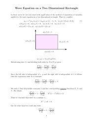
One of the simplest examples of a hyperbolic equation is the wave equation,<br />
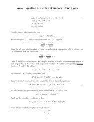
u xx = u tt , −∞
6.1. INTRODUCTION 7<br />
t<br />
u=0<br />
u=1/2<br />
u=1/2<br />
u=0 u=1<br />
x<br />
u=0<br />
The propagation of a disturbance in dimension 1.<br />
In general, for hyperbolic equations<br />
1. solutions are no smoother than data,<br />
2. there is a finite speed of propagation,<br />
3. solutions exhibit a strong dependence on spatial dimension,<br />
4. many quantities are preserved, and<br />
5. the Cauchy problem is well-posed.<br />
Parabolic <strong>Equations</strong><br />
The heat equation,<br />
u t (x, t) =∆u(x, t), x ∈ R n ,t>0<br />
is an example of a parabolic equation. If we think of u(x, t) as being the temperature at a<br />
point x at time t, this equation describes the flow or diffusion of heat. In view of our earlier<br />
discussion of the interpretation of the Laplacian, we see that if say, ∆u(x, t) < 0, then the<br />
temperature at position x is greater than that at surrounding points. From Fourier’s Law of<br />
Cooling, heat would ‘flow’ away from the position x, and from the differential equation we<br />
see that u t < 0, corresponding to the decrease in temperature at that point.<br />
The Cauchy problem for the heat equation on R n is<br />
u t =∆u(x, t), |x| < ∞, t>0.<br />
u(x, 0) = f(x).
8 CHAPTER 6. PARTIAL DIFFERENTIAL EQUATIONS<br />
The solution may be expressed as<br />
u(x, t) =<br />
∫<br />
1<br />
(4πt) n/2<br />
e −|x−y|2<br />
4t<br />
R n<br />
f(y) dy.<br />
From this formula, it is reasonable to expect the solution u(x, t) to be infinitely differentiable.<br />
In addtion, we see that if even if the data f is compactly supported, the temperature u(x, t)<br />
will be positive for all x when t > 0. These observations suggest the following general<br />
features of parabolic equations:<br />
1. solutions are smooth, and<br />
2. there is an infinite speed of conduction.<br />
6.2 Linear and Quasilinear equations of First Order<br />
|α|≤k<br />
In the study of linear partial differential equations a measure of the “strength” of a differential<br />
operator in a certain direction is provided by the notopn of charafcteristics. If<br />
L = ∑<br />
a α (x)∂ α is a linear differential operator of order k onΩinR n , then its characteristic<br />
form (or principal symbol) atx ∈ Ω is the homogeneous polynomial of degree k on R n<br />
defined by<br />
χ L (x, ξ) = ∑<br />
a α (x)ξ α .<br />
A vector ξ is characteristic for L at x if<br />
|α|=k<br />
χ L (x, ξ) =0.<br />
The characteristic variety is the set of all characteristic vectors ξ, i.e.,<br />
Char x (L) ={ξ ≠0:χ L (x, ξ) =0}.<br />
Definition 6.2.1. A hypersurface of class C k (1 ≤ k ≤∞) is a subset S ⊂ R n such that<br />
for each x 0 ∈ S there exists an open neighborhood V ⊂ R n of x 0 and a real-valued function<br />
ϕ ∈ C k (V ) such that ∇ϕ(x) ≠0for all x ∈ S ∩ V where<br />
S ∩ V = {x ∈ V : ϕ(x) =0}.<br />
Remark 6.2.2. Since, by definition, for each x 0 ∇ϕ(x 0 ) ≠ 0 we can apply the implicit<br />
function theorem (without loss of generality let us assume that ∂ xn ϕ(x 0 ) ≠0) to solve ϕ(x) =<br />
0 for x n = ψ(x ′ ) where x ′ =(x 1 , ··· ,x n−1 ) near x 0 . Thus a neighborhood of x 0 can be mapped<br />
to a piece of the hyperplane x n =0by x ↦→ (x ′ ,x n − ψ(x ′ )). The same neighborhood can be
6.2. LINEAR AND QUASILINEAR EQUATIONS OF FIRST ORDER 9<br />
also be represented in parametric form as the image of an open set in R n−1 (with coordinates<br />
x ′ ) under the map<br />
x ′ ↦→ (x ′ ,ψ(x ′ )).<br />
Thus x ′ can be thought of as giving local coordinates on S near x 0 .<br />
A hypersurface S is called characteristic for L at x if the normal vector ν(x) is in Char x (L)<br />
and S is called non-characteristic if it is not characteristic at any point.<br />
An important property of the characteristic variety is contained in the following:<br />
Let F be a smooth one-to-one mapping of Ω onto Ω ′ ⊂ R n and set y = F (x).<br />
Assume that the Jacobian matrix<br />
[ ] ∂yi<br />
J x = (x)<br />
∂x j<br />
is nonsingular for x ∈ Ω, so that {y 1 ,y 2 , ··· ,y n } is a coordinate system on Ω ′ .<br />
We have<br />
∂<br />
n∑ ∂y i ∂<br />
=<br />
∂x j ∂x j ∂y i<br />
i=1<br />
which we can write symbolically as ∂ x = Jx T ∂ y , where Jx<br />
T is the transpose of<br />
J x . The operator L is then transformed into<br />
L ′ = ∑ (<br />
a α F −1 (y) ) ( α<br />
J T F −1 (y) y) ∂ on Ω ′ .<br />
|α|≤k<br />
When this expression is expanded out, there will be some differentiations of J T F −1 (y) but<br />
such derivatives are only formed by “using up” some of the ∂ y on J T F −1 (y), so they do not<br />
enter in the computation of the principal symbol in the y coordinates, i.e., they do not enter<br />
the highest order terms. We find that<br />
χ L (x, ξ) = ∑<br />
( ) α<br />
a α (F −1 (y)) J T F −1 (y) ξ .<br />
|α|=k<br />
Now since F −1 (y) =x, on comparing with the expression<br />
χ L (x, ξ) = ∑<br />
a α (x)ξ α<br />
|α|=k<br />
we see that Char x (L) is the image of Char y (L ′ ) under the linear map J T F −1 (y) .
10 CHAPTER 6. PARTIAL DIFFERENTIAL EQUATIONS<br />
Note that if ξ ≠ 0 is a vector in the x j -direction (i.e., ξ i = 0 for i ≠ j), then ξ ∈ Char x (L)<br />
if and only if the coefficient of ∂j<br />
k in L vanishes at x. Now, given any ξ ≠ 0, by a rotation<br />
of coordinates we can arrange for ξ to lie in a coordinate direction. Thus the condition<br />
ξ ∈ Char x (L) means that, in some sense, L fails to be “genuinely kth order” in the ξ<br />
direction at x.<br />
L is said to be elliptic at x if Char x (L) =∅ and elliptic on Ω if it elliptic at each x ∈ Ω.<br />
Elliptic operators exert control on all derivatives of all order.<br />
Example 6.2.3. The first three examples are in R 2 as discussed above.<br />
1. L = ∂ 1 : Char x (L) ={ξ ≠0:ξ 1 =0}.<br />
2. L = ∂ 1 ∂ 2 : Char x (L) ={ξ ≠0:ξ 1 =0 or ξ 2 =0}.<br />
3. L = 1 2 (∂ 1 + i∂ 2 ): L is elliptic on R 2 .<br />
4. L =<br />
n∑<br />
∂j 2 (Laplace Operator): L is elliptic on R n .<br />
j=1<br />
n∑<br />
5. L = ∂ 1 − ∂j 2 (Heat Operator): Char x (L) ={ξ ≠0:ξ j =0, for j ≥ 2}.<br />
j=2<br />
6. L = ∂ 2 1 −<br />
n∑<br />
∂j<br />
2<br />
j=2<br />
(Wave Operator): Char x (L) ={ξ ≠0:ξ 2 j = ∑ n<br />
j=2 ξ2 j }.<br />
Remark 6.2.4. In the notation introduced in Definition 6.2.1 we say that a surface S is<br />
oriented if for each s ∈ S we have made a choice of a vector ν(x) which is orthogonal to S<br />
and is a continuously varying function of x. Such a vector is called a normal vector to S at<br />
x. OnS ∩ V = {x : ϕ(x) =0} we have<br />
ν(x) =± ∇ϕ(x)<br />
|∇ϕ(x)| .<br />
Thus ν(x) is a C k−1 function on S. If S is the boundary of a domain Ω then we usually<br />
choose the orientation so that ν points out of Ω.<br />
At this point we can also define the normal derivative by<br />
.<br />
∂ ν u = ν ·∇u.
6.2. LINEAR AND QUASILINEAR EQUATIONS OF FIRST ORDER 11<br />
Definition 6.2.5. A hypersurface S is called characteristic for L at x ∈ S if the normal<br />
vector ν(x) to S at x is in Char x (L), and S is called non-characteristic if it is not charateristic<br />
at any x in S.<br />
We now turn to the development for real first order systems. First recall the basic problem<br />
in ODEs is the IVP:<br />
Given a function F on say R 3 and (t 0 ,u 0 ) ∈ R 2 , find a function u(t) defined<br />
in a neighborhood of t 0 such that F (t, u, u ′ )=0and u(t 0 )=u 0 .<br />
In this disscussion we will consider the analog of this which is the initial value problem<br />
for a first order partial differential equation. We will focus on the linear and quasi-linear<br />
cases.<br />
Let us first consider the linear equation<br />
n∑<br />
a j ∂ j u + bu = f(x). (6.2.1)<br />
j=1<br />
where a j , b and f are assumed to be C 1 functions of x. If we denote by A the vector field<br />
then we have<br />
A(x) =(a 1 (x), ··· ,a n (x),<br />
Char x (L) ={ξ ≠0:A(x) · ξ =0}.<br />
That is, Char x (L) ∪{0} is the hyperplane orthogonal to A(x). From this we see that:<br />
A hypersurface S is characteristic at x if and only if A(x) is tangent to S at x.<br />
INITIAL VALUE PROBLEM: Find a solution u to (6.2.1) with given initial values<br />
u = ϕ on a given hypersurface S.<br />
If S is characteristic at a point x 0 , then the quantity ∑ a j (x 0 )∂ j u(x 0 ) is completely<br />
determined as a certain directional derivative of ϕ along S at x 0 . For this reason it may<br />
not be possible to make it equal to f(x 0 ) − b(x 0 )u(x 0 ). As an example, if the equation is<br />
∂ 1 u = 0 and S is the hyperplane x n = 0, we cannot have u = ϕ on S unless ∂ 1 ϕ =0.<br />
Namely, consider the case of R 2 . The general solution is given by u(x 1 ,x 2 )=f(x 2 ) where f<br />
is arbitrary. But if S corresponds to x 2 = 0 then the solution must satisfy u(x 1 , 0) = φ(x 1 )<br />
and the only choice is that ϕ ≡ 0.<br />
Thus to make the initial value problem well behaved, we must assume that S is noncharacteristic.<br />
It turns out that to solve for u it is useful to compute the integral curves of<br />
the vector field A(x).
12 CHAPTER 6. PARTIAL DIFFERENTIAL EQUATIONS<br />
Definition 6.2.6. The integral curves of the vector field A(x) are, by definition, the parameterized<br />
curves x(t) that satisfy the system of ODEs<br />
dx<br />
dt = A(x), i.e., dx j<br />
dt = a j(x), j =1, 2, ··· ,n. (6.2.2)<br />
Along such a curve a soution u of the equation (6.2.1) must satisfy<br />
du<br />
dt =<br />
n∑<br />
j=1<br />
∂u<br />
∂x j<br />
dx j<br />
dt = ∑ a j ∂ j u = f − bu. (6.2.3)<br />
That is, along such a curve a solution u of the equation (6.2.1) will satisfy the ODE<br />
du<br />
= f − bu. (6.2.4)<br />
dt<br />
By the fundamental existence uniqueness theorem from ODEs, through each point x 0 of S<br />
there passes a unique integral curve x(t) ofA, namely the solution of (6.2.2) with x(0) =<br />
x 0 . Along this curve the solution u of (6.2.1) must also be a solution of the ODE (6.2.4)<br />
with u(0) = ϕ(x 0 ). Moreover, since A is non-characteristic, x(t) ∉ S (at least for |t| ≠0<br />
sufficiently small) and the curves x(t) fill out a neighborhood of S. The same result as stated<br />
in Theorem 6.2.7 is given in the simpler case of R 2 in Subsection 6.2.1 (see, in particular,<br />
Theorem 6.2.14).<br />
Theorem 6.2.7. Assume that S is a hypersurface of class C 1 which is non-characteristic<br />
for (6.2.1), and that the functions a j , b, f, and ϕ are C 1 and real-valued. Then for any<br />
sufficiently small neighborhood Ω of S in R n there is a unique solution u ∈ C 1 of (6.2.1) that<br />
satisfies u = ϕ on S.<br />
This theorem is a special case of the corresponding result for quasi-linear equations so<br />
we will defer the proof of this result to the proof of the following more general result (see<br />
Theorem 6.2.7).<br />
Consider a first order quasi-linear equation<br />
n∑<br />
a j (x, u)∂ j u = b(x, u). (6.2.5)<br />
j=1<br />
In this case, we consider variables (x 1 , ··· ,x n ,u) ∈ R n+1 and note that if u is a function<br />
of x, then the normal to the graph of u (i.e., (x, u(x)) ∈ R n+1 )inR n+1 is proportional to<br />
⃗v =(∂ 1 u, ···∂ n u, −1). So (6.2.5) says that<br />
A(x, u) =(a 1 (x, u), ··· ,a n (x, u),b(x, u))
6.2. LINEAR AND QUASILINEAR EQUATIONS OF FIRST ORDER 13<br />
is tangent to the graph of y = u(x) at any point (since it is orthogonal to ⃗v).<br />
This suggests that we look at the integral curves of the vector field A(x, u) inR n+1 given<br />
by solving the equations<br />
dx j<br />
dt = a j(x, y), j=1, ··· ,n,<br />
dy<br />
dt<br />
= b(x, y). (6.2.6)<br />
As you will see, any graph y = u(x) inR n+1 which is the union of an (n − 1)-parameter<br />
family of these integral curves will define a solution of (6.2.5). Conversely, suppose that u is<br />
a solution of (6.2.5). If we solve the equations<br />
dx j<br />
dt = a j(x, u(x)),<br />
x j (0)=(x 0 ) j<br />
to obtain a curve x(t) passing through x 0 , and then set y = u(x(t)), we have<br />
dy<br />
dt =<br />
n∑<br />
j=1<br />
∂ j u dx j<br />
dt =<br />
n∑<br />
a j (x, u)∂ j u = b(x, u).<br />
j=1<br />
Thus if the graph y = u(x) intersects an integral curve of A in one point (x 0 ,u(x 0 )), it<br />
contains the whole curve.<br />
Suppose we are given intial data u = ϕ on a hypersurface S in R n . If we form the<br />
submanifold<br />
S ∗ = {(x, ϕ(x)) : x ∈ S}<br />
of R n+1 , the graph of the solution should be the hypersurface (in R n+1 ) generated by the integral<br />
curves of A passing through S ∗ . Again, we need to assume that S is non-characteristic<br />
in some sense. This is more complicated than the linear case because a j depend on u as well<br />
as x. We need the following geometric interpretation:<br />
For x ∈ S, the vector field A(x, ϕ(x)) = ( a 1 (x, ϕ(x)), ··· ,a n (x, ϕ(x)) ) should not<br />
be tangent to S at x. Note that this condition involves ϕ as well as S.<br />
If S is represented parametrically by a mapping g : R n−1 → R n and we take coordinates<br />
s =(s 1 , ··· ,s n−1 ) ∈ R n−1 , so that g(s) =(g 1 (s), ··· ,g n (s)) , then the above condition can<br />
be expressed as<br />
⎛<br />
⎞<br />
∂g 1 ∂g 1<br />
··· a 1 (g(s),φ(g(s)))<br />
∂s 1 ∂s n−1<br />
det<br />
⎜ . .<br />
.<br />
⎟ ≠0. (6.2.7)<br />
⎝∂g n ∂g n<br />
⎠<br />
··· a n (g(s),φ(g(s)))<br />
∂s 1<br />
∂s n−1
14 CHAPTER 6. PARTIAL DIFFERENTIAL EQUATIONS<br />
Theorem 6.2.8. Suppose that S is a C 1 hypersurface and a j , b and φ are C 1 real valued<br />
functions. Suppose that the vector field V =(a 1 (x, φ(x)), ··· ,a n (x, φ(x))) is not tangent to<br />
S at any x ∈ S (this is the noncharacteristic condition). Then there is a unique solution<br />
u ∈ C 1 of<br />
n∑<br />
a j (x, u)∂ j u = b(x, u)<br />
j=1<br />
in a neighborhood Ω of S such that u = φ on S.<br />
The proof of this result is constructive.<br />
Proof. The uniqueness follows from the discussion above which states that u must be the<br />
union of integral curves of A in Ω passing through S ∗ .<br />
Now any hypersurface S can be covered by by open sets on which it admits a parametric<br />
representation x = g(s), with s ∈ R n−1 . If we solve the problem on each such open set,<br />
by uniqueness the local solutions must agree on the overlap of the open sets and hence<br />
patch together to give a solution for all of S. It therefore suffices to assume that S is given<br />
parametrically by x = g(s) with s ∈ R n−1 .<br />
For each s ∈ R n−1 , consider the initial value problem<br />
∂x j<br />
∂t (s, t) =a j(x, y), j=1, ··· ,n,<br />
∂y<br />
(s, t) =b(x, y), (6.2.8)<br />
∂t<br />
x j (s, 0) = g j (s),<br />
y(s, 0) = ϕ(g(s)).<br />
Here s is a parameter vector, so we have a system of ODEs in t. By the fundamental existence<br />
uniqueness theorem for ODEs, there exists a unique solution (x, y) defined for small t, and<br />
(x, y) isaC 1 function of s and t jointly. By the non-characteristic condition (6.2.7) and the<br />
inverse mapping theorem, the mapping (s, t) ↦→ (x, t) is invertible on some neighborhood Ω<br />
of S, yielding s and t as C 1 functions of x on Ω such that t(x) =0andg(s(x)) = x when<br />
x ∈ S. Now set<br />
u(x) =y(s(x),t(x)).<br />
We have u = ϕ on S, and we claim that u satisfies (6.2.5). By the chain rule and the
6.2. LINEAR AND QUASILINEAR EQUATIONS OF FIRST ORDER 15<br />
fact that ∂s k<br />
∂t = 0, since s k and t are functionally independent, and ∂t<br />
∂t<br />
(<br />
n∑ ∂u<br />
n∑ n−1<br />
)<br />
∑ ∂u ∂s k<br />
a j = a j + ∂u ∂t<br />
∂x<br />
j=1 j ∂s<br />
j=1<br />
k ∂x j ∂t ∂x j<br />
k=1<br />
This completes the proof.<br />
=<br />
=<br />
=<br />
∑n−1<br />
k=1<br />
∑n−1<br />
k=1<br />
∑n−1<br />
k=1<br />
∂u<br />
∂s k<br />
∂u<br />
∂s k<br />
n∑<br />
j=1<br />
n∑<br />
j=1<br />
∂u<br />
∂s k<br />
∂s k<br />
=0+ ∂u<br />
∂t = b.<br />
∂s k<br />
a j + ∂u<br />
∂x j ∂t<br />
∂s k ∂x j<br />
∂x j ∂t + ∂u<br />
∂t<br />
∂t + ∂u ∂t<br />
∂t ∂t<br />
n∑<br />
j=1<br />
a j<br />
∂t<br />
∂x j<br />
n∑<br />
j=1<br />
∂x j<br />
∂t<br />
∂t<br />
∂x j<br />
= 1 we have<br />
Example 6.2.9. In R 3 solve the linear initial value problem Lu = x 1 ∂ 1 u+2x 2 ∂ 2 +∂ 3 u =3u<br />
with u = ϕ(x 1 ,x 2 ) on the plane x 3 =0.<br />
Solvability: We could observe that the solvability condition is satisfied by considering The<br />
vector field A(x) =(x 1 , 2x 2 , 1) and the characteristic manifold<br />
Char x (L) ={ξ =(ξ 1 ,ξ 2 ,ξ 3 ) ≠0:A(x) · ξ =0}.<br />
We note that the initial surface S in this case is x 3 = 0 with constant normal vector ν =<br />
(0, 0, 1). In the present case we see that<br />
A(x) · ν =1≠0<br />
so the surface is non-characteristic.<br />
We could also note that with s =(s 1 ,s 2 ) ∈ R 3−1 and<br />
g(s) =(g 1 (s),g 2 (s),g 3 (s))=(s 1 ,s 2 , 0)<br />
paramterizing the surface S we have for (6.2.7)<br />
⎛<br />
1 0 s 1<br />
⎞<br />
det ⎝0 1 2s 2<br />
⎠ = ϕ(s 1 ,s 2 ).<br />
0 0 ϕ(s 1 ,s 2 )
16 CHAPTER 6. PARTIAL DIFFERENTIAL EQUATIONS<br />
So under the assumption that ϕ(s 1 ,s 2 ) ≠ 0 we can solve the problem.<br />
Solution:In the present case the initial value problem (6.2.2) (see also (6.2.6) and (6.2.8))<br />
gives<br />
dx 1<br />
dt = x dx 2<br />
1,<br />
dt =2x dx 3<br />
2,<br />
dt =1, du<br />
dt =3u,<br />
with initial conditions<br />
(x 1 ,x 2 ,x 3 ,u) ∣ t=0<br />
=(s 1 ,s 2 , 0,φ(s 1 ,s 2 )).<br />
Solving this system of ODEs yields<br />
x 1 = s 1 e t ,x 2 = s 2 e 2t ,x 3 = t, u = ϕ(s 1 ,s 2 )e 3t .<br />
The next step is to invert the first three equations to obtain s 1 , s 2 and t<br />
t = x 3 , s 1 = x 1 e −x 3<br />
, s 2 = x 2 e −2x 3<br />
.<br />
Thus we find that<br />
u = ϕ(x 1 e −x 3<br />
,x 2 e −2x 3<br />
) e 3x 3<br />
.<br />
Example 6.2.10. Let us now consider a quasi-linear example in R 2 and we want to solve<br />
u∂ 1 u + ∂ 2 u = 1 with u = 1 2 s on the segment x 1 = x 2 = s, 0
6.2. LINEAR AND QUASILINEAR EQUATIONS OF FIRST ORDER 17<br />
6.2.1 Special Case: Quasilinear <strong>Equations</strong> in R 2<br />
As a special case let us consider n = 2, i.e., let us consider first order quasi-linear (or linear)<br />
equations in two variables in the form<br />
a(x, y, u) ∂u + b(x, y, u)∂u<br />
∂x ∂y<br />
= c(x, y, u). (6.2.9)<br />
For this example we adhere to common practice and refer to the variables as x and y or x<br />
and t, depending on the given problem, instead of x 1 and x 2 . Also in this case it is often<br />
useful to use the notations<br />
u x = ∂u<br />
∂x ,u y = ∂u<br />
∂y ,u t = ∂u<br />
∂t , etc.<br />
for the various partial derivatives.<br />
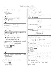
Let u = u(x, y) be a solution (also refered to as a solution surface. The vector (u x ,u y , −1)<br />
is normal to the surface u(x, y) − u = 0 and the equation (6.2.9) expresses the orthogonality<br />
condition<br />
A(x, y, u) · (u x ,u y , −1)=0, A(x, y, u) ≡ (a(x, y, u),b(x, y, u),c(x, y, u)). (6.2.10)<br />
u<br />
(u x ,u y , −1)<br />
(a, b, c)<br />
u = u(x, y)<br />
y<br />
x<br />
Solution Surface<br />
To solve (6.2.9) amounts to constructing a surface such that the normal to the surface<br />
satisfys the orthogonality condition (6.2.10). This is the same as saying that we seek a<br />
surface u = u(x, y) such that the tangent plane to the surface at (x, y, u) contains the<br />
vector (a(x, y, u),b(x, y, u),c(x, y, u)). More specifically, since we are really interested in the
18 CHAPTER 6. PARTIAL DIFFERENTIAL EQUATIONS<br />
initial value problem, we seek a solution of (6.2.9) that contains a given curve, say C 0 given<br />
parametrically by ( x 0 (s),y 0 (s),u 0 (s) ) . Recall that a three dimensional surface (in our case<br />
the solution surface u = u(x, y)) can be represented (at least locally) parametrically as a two<br />
parameter family<br />
(<br />
x(s, t),y(s, t),u(s, t)<br />
)<br />
.<br />
In this way we see that a solution surface is built-up from a two parameter family of curves<br />
(<br />
x(s, t),y(s, t),u(s, t)<br />
)<br />
. And , in order that the initial values be achieved we need<br />
(<br />
x(s, 0),y(s, 0),u(s, 0)<br />
)<br />
=<br />
(<br />
x0 (s),y 0 (s),u 0 (s) ) .<br />
If these curves lie on a solution surface, then tangent vectors to the curves must lie in the<br />
tangent plane to the surface at the point. This means that for a fixed s the curves (in t)<br />
must satisfy the equations<br />
dx<br />
(s, t) =a(x, y, u),<br />
dt x(s, 0) = x 0(s),<br />
dy<br />
dt (s, t) =b(x, y, u), y(s, 0) = y 0(s), (6.2.11)<br />
du<br />
(s, t) =c(x, y, u),<br />
dt u(s, 0) = u 0(s).<br />
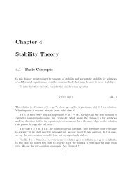
(<br />
x0 (s),y 0 (s),u 0 (s) )<br />
u<br />
(u x ,u y , −1)<br />
( x(s, τ),y(s, τ ),u(s, τ )<br />
)<br />
(a, b, c)<br />
y<br />
x<br />
characteristic<br />
(<br />
x0 (s),y 0 (s) )<br />
Solution Surface and Characteristic<br />
If the vector field A were tangent to the curve C 0 , then a solution of (6.2.11) would<br />
coincide with C 0 and our method for constructing a surface would fail. We will see that this<br />
problem can be avoided by not perscribing data on the curve with<br />
dx<br />
dt = a,<br />
dy<br />
dt = b.
6.2. LINEAR AND QUASILINEAR EQUATIONS OF FIRST ORDER 19<br />
Such a curve is called a characteristic curve. To construct a solution surface we first find<br />
x = x(s, t), y = y(s, t), u = u(s, t)<br />
and then solve the two equations x = x(s, t) and y = y(s, t) for s and t in terms of x and y.<br />
In order to guarantee that this can be done requires a result from advanced calculus – the<br />
inverse function theorem which states:<br />
If x = x(s, t) and y = y(s, t) are C 1 maps in a neighborhood of a point (s 0 ,t 0 ),<br />
the Jacobian<br />
⎛ ⎞<br />
∂x ∂x<br />
⎜ ⎟∣<br />
|J| = det ⎜ ∂t<br />
⎝∂y<br />
∂t<br />
∂s⎟<br />
∂y⎠<br />
∣<br />
∂s<br />
∣<br />
(s0 ,t 0 )<br />
≠0.<br />
and, in addition, x 0 = x(s 0 ,t 0 ) and y 0 = y(s 0 ,t 0 ), then there exists a neighborhood<br />
R of (s 0 ,t 0 ) and there exists unique C 1 mappings<br />
and<br />
s = s(x, y), t = t(x, y)<br />
s = s(x 0 (s),y 0 (s)),<br />
0=t(x 0 (s),y 0 (s))<br />
With this we can construct our solution surface as<br />
and<br />
u = u(s, t) =u(s(x, y),t(x, y)) = u(x, y),<br />
u 0 (s) =u(s, 0) = u(s(x 0 (s),y 0 (s)),t(x 0 (s),y 0 (s))) = u(x 0 ,y 0 ).<br />
Example 6.2.11. Solve<br />
We first seek solutions of<br />
xu x +(x + y)u y = u +1, u(x, 0) = x 2 .<br />
dx<br />
dt = x,<br />
In this case we can parameterize C 0 by<br />
dy<br />
dt = x + y,<br />
du<br />
dt = u +1.<br />
x 0 (s) =s, y 0 (s) =0, u 0 (s) =s 2
20 CHAPTER 6. PARTIAL DIFFERENTIAL EQUATIONS<br />
and the initial conditions are<br />
x(s, 0) = x 0 (s) =0,y(s, 0) = y 0 (s) =0,u(s, 0) = u 0 (s) =s 2 .<br />
Thus we solve<br />
x ′ = x<br />
x(s, 0) = s<br />
}<br />
⇒<br />
x(s, t) =se t<br />
y ′ − y = se t<br />
y(s, 0)=0<br />
}<br />
⇒<br />
y(s, t) =ste t<br />
du<br />
u +1 = dt<br />
u(s, 0) = s 2 ⎫<br />
⎬<br />
⎭ ⇒ u(s, t) =(1+s2 )e t − 1.<br />
Since x = se t and y = ste t we see that t = y x and hence s = xe−y/x .Thus<br />
u(x, y) =(1+x 2 e −2y/x )e y/x − 1=e y/x + x 2 e −y/x − 1, for x ≠0.<br />
Example 6.2.12. (Unidirectional Wave Motion) In this linear example we seek a function<br />
u = u(x, t) such that<br />
∂u<br />
∂t + c∂u =0, (6.2.12)<br />
∂x<br />
u(x, 0) = F (x). (6.2.13)<br />
We first seek solutions of<br />
dx<br />
dτ = c,<br />
dt<br />
dτ =1,<br />
du<br />
dτ =0,<br />
subject to<br />
x(s, 0) = s, t(s, 0)=0, u(s, 0) = F (s).<br />
Thus we obtain<br />
x = cτ + s, t = τ, u = F (s).<br />
Solving for s and τ in terms of x and t we have<br />
We then get<br />
s = x − ct,<br />
τ = t<br />
u(x, t) =u(s(x, t),τ(x, t)) = F (x − ct).
6.2. LINEAR AND QUASILINEAR EQUATIONS OF FIRST ORDER 21<br />
Example 6.2.13. Let us now consider an example in which data is prescribed on characteristics.<br />
In this linear example we seek a function u = u(x, y) such that<br />
We first seek solutions of<br />
subject to<br />
Thus we obtain<br />
dx<br />
dt = x,<br />
x ∂u<br />
∂x + y ∂u<br />
∂y = u + 1 (6.2.14)<br />
u(x, x) =x 2 . (6.2.15)<br />
dy<br />
dt = y,<br />
du<br />
dt = u +1,<br />
x(s, 0) = s, y(s, 0) = s, u(s, 0) = s 2 .<br />
x = se t , y = se t , u = s 2 e t + e t − 1.<br />
In this example it is not possible to solve for s and t in terms of x and y. Not that A(x, y) =<br />
(x, y) and the characteristic manifold<br />
Char (x,y) (L) ={ξ =(ξ 1 ,ξ 2 ) ≠0:A(x, y) · ξ =0}.<br />
We note that the initial curve S in this case is x = y with constant normal vector ν =(1, −1).<br />
In the present case we see that<br />
so the curve is a characteristic.<br />
A(x, x) · ν = x − x =0<br />
Within the context of these examples in R 2<br />
solvability condition (6.2.7) as<br />
we can restate Theorem 6.2.8 with the<br />
Theorem 6.2.14. Suppose a(x, y, u), b(x, y, u), c(x, y, u) are C 1 in Ω ⊂ R 3 , C 0 is C 1 initial<br />
curve given by (x 0 (s),y 0 (s),u 0 (s)) ⊂ Ω and<br />
( )<br />
a(x0 (s),y<br />
det<br />
0 (s),u 0 (s)) x ′ 0(s)<br />
b(x 0 (s),y 0 (s),u 0 (s)) y 0(s)<br />
′ ≠0.<br />
Then there exists a unique C 1 solution of<br />
a(x, y, u)u x + b(x, y, u)u y = c(x, y, u),<br />
with<br />
u(x 0 (s),y 0 (s)) = u 0 (s).
22 CHAPTER 6. PARTIAL DIFFERENTIAL EQUATIONS<br />
Proof. Our regularity assumptions guarantee that the initial value problem<br />
dx<br />
dt<br />
dy<br />
dt<br />
du<br />
dt<br />
= a(x, y, u), x(s,<br />
= b(x, y, u), y(s,<br />
= c(x, y, u), u(s,<br />
0) = x 0(s)<br />
0) = y 0(s)<br />
0) = u 0(s)<br />
has a unique local solution that is C 1 in t and s. By our hypotheses<br />
⎛ ⎞<br />
∂x ∂x<br />
|J| = det ⎜ ∂t ∂s<br />
⎟<br />
⎝∂y<br />
∂y⎠<br />
=<br />
∣ a(x 0(s),y 0 (s),u 0 (s)) x ′ 0(s)<br />
b(x 0 (s),y 0 (s),u 0 (s)) y 0(s)<br />
′<br />
∣<br />
∂t ∂s t=0<br />
∣ ≠0<br />
Thus |J| ≠ 0 in a neighborhood of the initial curve C 0 and by the inverse function theorem<br />
we can solve for<br />
s = s(x, y), t = t(x, y)<br />
and s = s(x 0 (s),y 0 (s)),<br />
0=t(x 0 (s),y 0 (s)), so we can define<br />
u = u(x, y) =u(s(x, y),t(x, y)).<br />
We first note that u satisfies the initial conditions:<br />
u(x 0 (s),y 0 (s)) = u(s, 0) = u 0 (s).<br />
Furthermore, by the chain rule<br />
(<br />
)<br />
∂s<br />
au x + bu y = a u s<br />
∂x + u ∂t<br />
t<br />
∂x<br />
(<br />
∂s<br />
+ b u s<br />
=(as x + bs y )u s +(at x + bt y ))u t .<br />
)<br />
∂y + u ∂t<br />
t<br />
∂y<br />
Now by our construction of x, y, and since x t = a, y t = b, wehave<br />
and<br />
as x + bs y = s x x t + s y y t = ∂s<br />
∂t =0,<br />
at x + bt y = s x x t + t y y t = ∂t<br />
∂t =1
6.2. LINEAR AND QUASILINEAR EQUATIONS OF FIRST ORDER 23<br />
and so<br />
au x + bu y = c.<br />
Recall that in the case of a differential equation in R 2 a solution surface is a surface in<br />
R 3 which (at least locally) can be parameterized by a two parameter family. Thus what<br />
we have shown is that the collection of all characteristic curves thorugh C 0 gives a solution<br />
surface. Uniqueness will follow by arguing that any solution surface is essentially a collection<br />
of characteristic curves. In particular let u(x, y) be a solution of the equation and fix a point<br />
P 0 (x 0 ,y 0 ,z 0 ) on the surface. Let γ :(x(t),y(t),z(t)) be the curve through P 0 determined by<br />
dx<br />
dt = a(x, y, u(x, y)), x(0) = x 0<br />
dy<br />
dt = b(x, y, u(x, y)), y(0) = y 0<br />
z(t) =u(x, y), z(0) = z 0 .<br />
Then along this curve<br />
dz<br />
dt = u dx<br />
x<br />
dt + u dy<br />
y<br />
dt = au x + bu y = c<br />
since u is a solution. Thus we see that γ is the characteristic curve through P 0 . In other<br />
words, a solution is always a union of characteristic curves. Through any point on a solution<br />
surface there is a unique characteristic curve.<br />
Therefore if C 0 is not a characteristic curve, there is a unique solution surface that<br />
contains it. If, on the other hand, C 0 is a characteristic curve then<br />
x ′ 0(s) =a(x 0 (s),y 0 (s),ϕ ( s))<br />
y 0(s) ′ =b(x 0 (s),y 0 (s),ϕ ( s))<br />
which contradicts |J| ≠0.<br />
Remark 6.2.15. The above discussion shows that if C 0 were a characteristic curve we could<br />
construct infinitely many solutions containing C 0 . Namely, take any curve C 1 that meets C 0<br />
in a point P 0 and such that |J| ≠0on C 1 . Then construct the solution surface through C 1 .<br />
As discussed above, this solution surface must contain the characteristic curve C 0 .
24 CHAPTER 6. PARTIAL DIFFERENTIAL EQUATIONS<br />
P 0<br />
C 0<br />
C 1<br />
Example 6.2.16. Recall the Example 6.2.12<br />
Solution Surface for Each Curve C 1<br />
u t + cu x =0,<br />
u(x, 0) = F (x)<br />
with solution given by<br />
u(x, t) =F (x + ct).<br />
We note that the initial surface is t = 0 and the characteristics are determined by<br />
dx<br />
dτ = c, x(s, 0) = s, dt<br />
=1,t(s, 0)=0, ⇒ t(s, τ) =τ, x(s, τ) =cτ + s, ⇒ x − ct = s.<br />
dτ<br />
Thus we see that the solution is constant along characterisitics, i.e., (x, t) on a characteristic<br />
means that x − ct = s = constant and the solution is given by u(x, t) =F () and u is<br />
constant on a characteristic, i.e., a line x − ct = s for s ∈ R.<br />
A generalization of this problem is the case in which c = c(x, t). Then the characteristics<br />
are determined by<br />
and along this curve<br />
dx<br />
dτ<br />
= c(x, t), x(s,<br />
0) = s, dt<br />
dτ<br />
=1,t(s, 0)=0,<br />
du<br />
dt (x(t),t)=u dx<br />
x<br />
dt + u dt<br />
t<br />
dt = u xc(x(t),t)+u t ≡ 0.
6.2. LINEAR AND QUASILINEAR EQUATIONS OF FIRST ORDER 25<br />
Hence u is constant on a characteristic.<br />
Consider, for example,<br />
The characteristics are determined by<br />
which yields the parabolas<br />
u t +2tu x =0, u(x, 0) = e −x2 .<br />
dx<br />
dt =2t<br />
x = t 2 + k, k constant .<br />
The characteristic through a point (ξ,0) is x = t 2 + ξ. Since u is constant on this curve we<br />
have<br />
u(x, t) = exp(−ξ 2 )=e −(x−t2 ) 2 .<br />
Example 6.2.17. In the study of fluid flow an important physical characteristic is the<br />
formation of shock waves. The simplest example of the formation of shocks can be witnessed<br />
in the study of certain quasi-linear equations in R 2 called hyperbolic conservation laws.<br />
These are equations of the form<br />
subject to initial conditions<br />
The characteristics are determined by<br />
Along this curve<br />
u t + c(u)u x =0, x ∈ R, t>0 (6.2.16)<br />
u(x, 0) = ϕ(x), x ∈ R. (6.2.17)<br />
dx<br />
dt = c(u)<br />
du<br />
dt (x(t),t)=u x(x(t),t) dx<br />
dt + u t(x(t),t) dt<br />
dt = u xc(u)+u t ≡ 0.<br />
Hence u is constant on a characteristic. The characteristics are straight lines since<br />
d 2 x<br />
dt 2<br />
= d dt<br />
( ) dx<br />
= d dt dt c(u) =c′ (u) du<br />
dt =0,
26 CHAPTER 6. PARTIAL DIFFERENTIAL EQUATIONS<br />
which implies that x = C 1 t + C 2 . Now since u is constant on a characteristic, then on a<br />
characteristic, say the characteristic passing through (ξ,0),<br />
dx<br />
dt<br />
= c(u(x(t),t)) = c(u(ξ,0)) = c(ϕ(ξ)).<br />
Thus we see that the slope of the characteristics depend on c(u) and the initial data. The<br />
equation for the characteristic passing through (ξ,0) is given by<br />
and the solution on this line is given by<br />
where x = c ( ϕ(ξ) ) t + ξ.<br />
x = c ( ϕ(ξ) ) t + ξ,<br />
u(x, t) =ϕ(ξ) =ϕ(x − c(ϕ(ξ))t)<br />
t<br />
(x, t)<br />
(ξ,0)<br />
x<br />
Characteristic through (ξ,0)<br />
Example 6.2.18. One particularly famous example of a hyperbolic conservation law which<br />
is often used as a one dimensional model for the Navier-Stokes equations is the Burgers’<br />
equation given by<br />
Let us consider (6.2.18) subject to initial conditions<br />
u t + uu x =0, x ∈ R, t>0. (6.2.18)<br />
⎧<br />
⎨ 2, x < 0<br />
u(x, 0) = ϕ(x) = 2 − x, 0 ≤ x ≤ 1 . (6.2.19)<br />
⎩<br />
1, x > 1<br />
For x1 the slope is 1.
6.2. LINEAR AND QUASILINEAR EQUATIONS OF FIRST ORDER 27<br />
Let us demonstrate that u − ϕ(x − c(u)t) = 0 implicitly defines a solution u(x, t) ofthe<br />
equation. First, differentiating with respect to x, wehave<br />
u x = ϕ ′ (x − c(u)t) [ x − c(u)t ] = x ϕ′ (x − c(u)t) [ 1 − c ′ (u)u x t ]<br />
and we can solve for u x<br />
u x =<br />
ϕ ′ (x − c(u)t)<br />
1+tc ′ (u)ϕ ′ (x − c(u)t) . (6.2.20)<br />
Now we differentiate with respect to t, to obtain<br />
u t = ϕ ′ (x − c(u)t) [ x − c(u)t ] = t −ϕ′ (x − c(u)t) [ tc ′ (u)u t + c(u) ]<br />
and we can solve for u t<br />
u t = −c(u)ϕ′ (x − c(u)t)<br />
1+tc ′ (u)ϕ ′ (x − c(u)t) . (6.2.21)<br />
So, combining (6.2.20) and (6.2.21), we have<br />
u t + c(u)u x =<br />
−c(u)ϕ′ (x − c(u)t)<br />
1+tc ′ (u)ϕ ′ (x − c(u)t) + c(u) ϕ ′ (x − c(u)t)<br />
1+tc ′ (u)ϕ ′ (x − c(u)t)<br />
= −c(u)ϕ′ (x − c(u)t)+c(u)ϕ ′ (x − c(u)t)<br />
=0.<br />
1+tc ′ (u)ϕ ′ (x − c(u)t)<br />
and<br />
u(x, 0) = ϕ(x − 0) = ϕ(x).<br />
t<br />
t =1<br />
(ξ,0)<br />
x<br />
Solution Exists Only for t1 since the characteristics<br />
cross beyond that line and the values on u on the intersecting characteristics are different –
28 CHAPTER 6. PARTIAL DIFFERENTIAL EQUATIONS<br />
thus, as a function, u is not well defined. More specifically, recall that our solution is defined<br />
by<br />
u(x, t) =ϕ(ξ) where x = ϕ(ξ)t + ξ.<br />
The characteristics are described by<br />
⎧<br />
⎨ 2t + ξ, ξ < 0<br />
x = (2 − ξ)t + ξ, 0 ≤ ξ ≤ 1 .<br />
⎩<br />
t + ξ, ξ > 1<br />
We can compute that the characteristics intersect at<br />
((2 − ξ)t + ξ) ∣ ∣<br />
ξ=0<br />
=(t + ξ) ∣ ∣<br />
ξ=1<br />
,<br />
or 2t =1+t, i.e., t =1. Fort1)<br />
t<br />
t =1<br />
x = t +1<br />
x =2t<br />
u =2<br />
(ξ,0)<br />
u =1<br />
x<br />
Solution<br />
If 0 ≤ ξ ≤ 1 the characteristic passing through (ξ,0) is x =(2− ξ)t + ξ which implies<br />
ξ =(x − 2t)/(1 − t) and so<br />
( ) x − 2t<br />
u(x, t) =2− = 2 − x , 2t ≤ x ≤ t +1, t < 1.<br />
1 − t 1 − t<br />
u<br />
t =1<br />
u =2<br />
t<br />
u =1<br />
x
6.2. LINEAR AND QUASILINEAR EQUATIONS OF FIRST ORDER 29<br />
Solution<br />
At t = 1 refered to as the “breaking time,” a “shock” develops. As an exercise you will<br />
show that for general c(u), the breaking time is given by<br />
t b = min<br />
ξ<br />
−1<br />
ϕ ′ (ξ)c ′ (ϕ(ξ)) ,t b > 0,<br />
at which<br />
1+c ′ (ϕ(ξ))ϕ ′ (ξ)t =0.
30 CHAPTER 6. PARTIAL DIFFERENTIAL EQUATIONS<br />
Exercise Set 1: First Order Linear and Quasi-Linear <strong>Equations</strong><br />
1. Solve the initial value problems<br />
(a) yz x − xz y =2xyz for z = t 2 on C: x = t, y = t, t>0.<br />
(b) zz x + yz y = x with z =2t on C: x = t, y = t, t ∈ R.<br />
2. Solve ∂ x u + ∂ y u = u with u = cos(x) when y =0.<br />
3. Solve x 2 ∂ x u + y 2 ∂ y u = u 2 with u = 1 when y =2x.<br />
4. Solve u∂ x u + ∂ y u = 1 with u = 0 when y = x. What happens in this problem if we<br />
replace u =0byu =1<br />
5. Solve u x + u y = u 2 with the initial condition u(x, 0) = h(x).<br />
6. Show that for the initial value problem,<br />
u t + c(u)u x =0,x∈ R, t > 0,<br />
u(x, 0) = φ(x)<br />
the breaking time will occur at the minimum value of t for which<br />
−1<br />
t b = min<br />
φ ′ (ξ)c ′ (φ(ξ))<br />
for which<br />
1+φ ′ (ξ)c ′ (φ(ξ))t =0.<br />
7. (a) Solve the initial value problem<br />
uu x + u t =0, u(x, 0) = f(x).<br />
(b) If f(x) =x, show that the solution exists for all t>0.<br />
(c) If f(x) =−x, show that a shock develops, that is, the solution blows up in finite<br />
time.<br />
⎧<br />
8. Let D be a constant and H the Heaviside function. Solve<br />
⎪⎨ u t + cu x =0,x∈ R,t>0,<br />
⎪⎩<br />
u(x, 0) = −H(−x)xe x/D<br />
if (c 0 is a constant)<br />
a) c(x) =c 0 (1 − x/L)<br />
b) c(x, t) =c 0 (1 − x/L − t/T ).
6.3. CHARACTERISTICS AND HIGHER ORDER EQUATIONS 31<br />
6.3 Characteristics and Higher Order <strong>Equations</strong><br />
6.3.1 Characteristics and Classification of 2nd Order <strong>Equations</strong><br />
L =<br />
n∑ ∂ 2<br />
a ij (x)<br />
(6.3.1)<br />
∂ xi ∂ xj<br />
i,j=1<br />
where a ij are real valued functions in Ω ⊂ R n and a ij = a ji . Fix a point x 0 ∈ Ω. The<br />
characteristic polynomial is given by<br />
We say that the operator L is:<br />
σ x0 (L, ξ) =<br />
n∑<br />
a ij (x 0 )ξ i ξ j (6.3.2)<br />
i,j=1<br />
1. Elliptic at x 0 if the quadratic form (6.3.2) is non-singular and definite, i.e., can be<br />
reduced by a real linear transformation to the form<br />
n∑<br />
ã i ξi 2 + l. o. t.<br />
i=1<br />
2. Hyperbolic at x 0 if the quadratic form (6.3.2) is non-singular and indefinite and can be<br />
reduced by a real linear transformation to a sum of n squares, (n − 1) of the same sign,<br />
i.e., to the form<br />
n∑<br />
ξ1 2 − ã i ξi 2 + l. o. t.<br />
i=2<br />
3. Ultra-Hyperbolic at x 0 if the quadratic form (6.3.2) is non-singular and indefinite and<br />
can be reduced by a real linear transformation to a sum of n squares, (n ≥ 4) with<br />
more than one terms of either sign.<br />
4. Parabolic at x 0 if the quadratic form (6.3.2) is singular, i.e., can be reduced by a real<br />
linear transformation to a sum of fewer than n squares, (not necessarily of the same<br />
sign).<br />
It can be shown that in the constant coefficient case a reduction to one of these forms is<br />
always possible with a simple constant matrix transformation of coordinates.<br />
The case of two independent variables and non-constant coefficients can also be analyzed.<br />
a ∂2 u<br />
∂x 2 +2b ∂2 u<br />
∂x∂y + c∂2 u<br />
∂y 2 + F (x, y, u, u x,u y ) = 0 (6.3.3)
32 CHAPTER 6. PARTIAL DIFFERENTIAL EQUATIONS<br />
where a = a(x, y), b = b(x, y), c = c(x, y) are C 2 real valued functions in Ω ⊂ R 2 and (a, b, c)<br />
doesn’t vanish at any point. Let us restrict to the linear case<br />
a ∂2 u<br />
∂x +2b ∂2 u<br />
2 ∂x∂y + u<br />
c∂2 ∂y + d∂u<br />
2 ∂x + e∂u + fu = g (6.3.4)<br />
∂y<br />
Example 6.3.1. Consider the one dimensional wave equation<br />
Let<br />
u xx − u yy =0.<br />
α = ϕ(x, y) =x + y, β = ψ(x, y) =x − y.<br />
So we have<br />
(α + β)<br />
(α − β)<br />
x =Φ(α, β) = , y =Ψ(α, β) = .<br />
2<br />
2<br />
We can express the solutions in terms of the (x, y) or(α, β) coordinates<br />
By the chain rule we have<br />
Thus we have<br />
u(x, y) =u(Φ(α, β), Ψ(α, β)) = U(α, β).<br />
u x = U α ϕ x + U β ψ x = U α + U β , (6.3.5)<br />
u xx = U αα +2U αβ + U ββ , (6.3.6)<br />
u y = U α ϕ y + U β ψ y = U α − U β , (6.3.7)<br />
u yy = U αα − 2U αβ + U ββ . (6.3.8)<br />
0=u xx − u yy =4U αβ , or U αβ =0.<br />
The general solution of this equation is given by<br />
which, in turn, implies<br />
U(α, β) =G(α)+F (β)<br />
u(x, y) =G(x + y)+F (x − y).<br />
This solution represents a pair of waves traveling at the same speed but in opposite directions.<br />
Returning to (6.3.4), if we introduce a nonsingular C 1 coordinate transformation<br />
{ α = ϕ(x, y)<br />
β = ψ(x, y),
6.3. CHARACTERISTICS AND HIGHER ORDER EQUATIONS 33<br />
i.e., the Jacobian is not zero<br />
|J| = det<br />
⎡<br />
⎢<br />
⎣<br />
∂α<br />
∂x<br />
∂β<br />
∂x<br />
⎤<br />
∂α<br />
∂y<br />
⎥<br />
∂β ⎦ ≠0.<br />
∂y<br />
Applying the chain rule we have<br />
u x = u α ϕ x + u β ψ x , u y = u α ϕ y + u β ψ y ,<br />
u xx = u αα ϕ 2 x +2u αβ ϕ x ψ x + u ββ ψx 2 + u α ϕ xx + u β ψ xx ,<br />
u yy = u αα ϕ 2 y +2u αβ ϕ y ψ y + u ββ ψy 2 + u α ϕ yy + u β ψ yy ,<br />
u xy = u αα ϕ x ϕ y + u αβ (ϕ x ψ y + ϕ y ψ x )+u ββ ψ x ψ y + u α ϕ xy + u β ψ xy .<br />
Then the equation (6.3.4) is transformed into a new equation of exactly the same form<br />
where<br />
ã ∂2 u<br />
∂α +2˜b ∂2 u<br />
2 ∂α∂β + ˜c ∂2 u ∂u<br />
+ ˜d<br />
∂β2 ∂α + ẽ ∂u<br />
∂β + ˜fu = ˜g (6.3.9)<br />
1. ã = aα 2 x +2bα x α y + cα 2 y<br />
2. ˜b = aα x β x + b(α x β y + α y β x )+cα y β y<br />
3. ˜c = aβx 2 +2bβ x β y + cβy<br />
2 (6.3.10)<br />
4. ˜d = aαxx +2bα xy + cα yy + dα x + eα y<br />
5. ẽ = aβ xx +2bβ xy + cβ yy + dβ x + eβ y<br />
6. ˜f = f and ˜g = g<br />
Furthermore, we have the following extremely important invariance<br />
˜D =(˜b 2 − ã˜c) =(b 2 − ac)J 2 = DJ 2 .<br />
With this we then obtain the following theorem. The proof is constructive.<br />
Theorem 6.3.2. D is positive, negative or zero if and only if ˜D is. Furthermore, we have<br />
1. D>0 implies Hyperbolic
34 CHAPTER 6. PARTIAL DIFFERENTIAL EQUATIONS<br />
2. D =0implies Parabolic<br />
3. D0 implies ã = ˜c =0<br />
2. D =0implies ã = ˜b =0<br />
3. D 0. If a = c = 0 we are done so we assume<br />
without loss of generality that a ≠ 0. We seek α = ϕ(x, y) and β = ψ(x, y) so that ã<br />
and ˜c are zero. We first note that the calculations (6.3.10) suggest that we consider an<br />
expression of the form<br />
av 2 x +2bv x v y + cv 2 y = 0 (6.3.11)
6.3. CHARACTERISTICS AND HIGHER ORDER EQUATIONS 35<br />
where v could represent either ϕ or ψ. We note that (6.3.11) can be factored into<br />
[ ( √ ) ][ ( √ ) ]<br />
−b + b2 − ac<br />
−b − b2 − ac<br />
a v x −<br />
v y v x −<br />
v y . (6.3.12)<br />
a<br />
a<br />
Thus from (6.3.12) we seek ϕ and ψ so that, for example,<br />
[ ( √ ) ]<br />
−b + b2 − ac<br />
ϕ x −<br />
ϕ y =0, (6.3.13)<br />
a<br />
and<br />
[<br />
ψ x −<br />
( √ ) ]<br />
−b − b2 − ac<br />
ψ y =0. (6.3.14)<br />
a<br />
With these choices (6.3.11) is satisfied with v given by ϕ and ψ. In addition we must<br />
impose a noncharacteristic solvability condition<br />
∣<br />
∂(ϕ, ψ) ∣∣∣∣<br />
∂(x, y) = ϕ x<br />
ψ x<br />
ϕ y<br />
ψ y<br />
∣ ∣∣∣∣<br />
( √ )<br />
−b + b2 − ac<br />
=<br />
ϕ y ψ y −<br />
a<br />
( −b −<br />
√<br />
b2 − ac<br />
a<br />
)<br />
ϕ y ψ y<br />
= 2 a<br />
√<br />
b2 − ac ϕ y ψ y ≠0. (6.3.15)<br />
A solution of (6.3.13) is found by solving<br />
dx<br />
dt =1,<br />
( √ )<br />
dy −b +<br />
dt = − b2 − ac<br />
,<br />
a<br />
dϕ<br />
dt =0.<br />
For this problem we take the initial conditions<br />
x 0 (s) =x 0 ,y 0 (s) =y 0 + s,<br />
ϕ 0 (s) =s.<br />
With this choice we find (in our earlier notation we used a and b which are not the<br />
same as those occuring in the present problem)<br />
∣ ∣∣∣∣∣∣ a x ′ 1 0<br />
0(s)<br />
∣b<br />
y 0(s)<br />
′ ∣ = ( √ )<br />
b − b2 − ac<br />
≠0. (6.3.16)<br />
1<br />
a ∣
36 CHAPTER 6. PARTIAL DIFFERENTIAL EQUATIONS<br />
Moreover,<br />
and so<br />
ϕ(s, t) =s<br />
ϕ s =1=ϕ x x s + ϕ y y s .<br />
If ϕ y = 0, then it follows from (6.3.13) that ϕ x = 0, a contradiction. Now, as we have<br />
learned in our earlier work, the condition (6.3.16) guarantees that we can solve for<br />
(s, t) in terms of (x, y) to obtain ϕ(x, y).<br />
Similarly, we can obtain ψ(x, y) by solving<br />
dx<br />
dt =1,<br />
( √ )<br />
dy b +<br />
dt = b2 − ac<br />
,<br />
a<br />
For this problem we take the initial conditions<br />
dψ<br />
dt =0.<br />
x 0 (s) =x 0 ,y 0 (s) =y 0 + s,<br />
ψ 0 (s) =s.<br />
Again, ψ(s, t) =s and as above ψ y ≠0. ThusJ ( (ϕ, ψ)/(x, y) ) ≠0.<br />
In summary we have found a change of coordinates α = ϕ(x, y), β = ψ(x, y) that<br />
reduces the equation to<br />
2˜bu αβ + l.o.t. = 0.<br />
It is easy to show that<br />
˜b =2<br />
( ac − b<br />
2<br />
a<br />
)<br />
ϕ y ψ y (6.3.17)<br />
and so ˜b ≠ 0 and we can divide by it to put (6.3.17) into the normal form<br />
Remark 6.3.4.<br />
u αβ = F (α, β, u, u α ,u β ).<br />
(a) The reduction to normal form is a local result.<br />
(b) The special initial curve can be replaced by any curve (x 0 (s),y 0 (s),ϕ 0 (s)) with<br />
ϕ 0 (s) =s and (x 0 (s),y 0 (s)) that specifies a curve in the xy-plane where the PDE<br />
is hyperbolic.<br />
(c) The curves ϕ(x, y) = constant, ψ(x, y) = constant are called characteristics of<br />
(6.3.4). Further, equation (6.3.11) is called the characteristic equation for the<br />
PDE.
6.3. CHARACTERISTICS AND HIGHER ORDER EQUATIONS 37<br />
(d) Note that the characteristics for the first order PDE’s for ϕ and ψ are determined<br />
by<br />
( √ )<br />
dx<br />
dt =1, dy b ±<br />
dt = b2 − ac<br />
a<br />
or<br />
( √ )<br />
dy b ±<br />
dx = b2 − ac<br />
.<br />
a<br />
But if ϕ(x, y) = constant and ϕ solves (6.3.13), then<br />
and so<br />
dy<br />
dx = −ϕ x<br />
ϕ y<br />
=<br />
ϕ x + ϕ y<br />
dy<br />
dx =0<br />
( b −<br />
√<br />
b2 − ac<br />
a<br />
)<br />
. (6.3.18)<br />
Hence the characteristics for a 2nd order PDE (6.3.4) coincide with the characteristics<br />
of the associated 1st order PDE (6.3.13) (Similarly for ψ).<br />
(e) In order to obtain the other hyperbolic form we set<br />
ξ = α + β,<br />
η = α − β<br />
so that<br />
and<br />
Thus we have<br />
α = ξ + η<br />
2 , β = ξ − η<br />
2 ,<br />
u α = u η η α + u ξ ξ α = u η + u ξ , u β = u η η β + u ξ ξ β = −u η + u ξ .<br />
u αβ =(−u ηη + u ηξ )+(−u ξη + u ξξ )=u ξξ − u ηη .<br />
Example 6.3.5. Consider the equation y 2 u xx − x 2 u yy = 0, x > 0, y > 0. Here<br />
b 2 − ac = x 2 y 2 > 0. The characteristics are given by ( see (6.3.18))<br />
( √ )<br />
dy b +<br />
dx = b2 − ac<br />
= x a y ,<br />
and<br />
( √ )<br />
dy b −<br />
dx = b2 − ac<br />
= − x a<br />
y .
38 CHAPTER 6. PARTIAL DIFFERENTIAL EQUATIONS<br />
Thus the characteristic curves are given by<br />
y 2 − x 2 = constant,<br />
y 2 + x 2 = constant.<br />
We take<br />
α = ϕ(x, y) =x 2 + y 2 , β = ψ(x, y) =x 2 − y 2 .<br />
We solve for x, y to obtain<br />
If we use (6.3.10) we find<br />
√ √<br />
α + β α − β<br />
x = , y = .<br />
2<br />
2<br />
˜b =8x 2 y 2 =2(α 2 − β 2 )<br />
˜d =2(y 2 − x 2 )=−2β<br />
ẽ =2(y 2 + x 2 )=2α<br />
and also<br />
u αβ =<br />
2β<br />
4(α 2 − β 2 ) u 2β<br />
α −<br />
4(α 2 − β 2 ) u β<br />
= βu a − αu β<br />
2(α 2 − β 2 ) .<br />
Example 6.3.6. Suppose that a, b, c, d, e, f in (6.3.4) are constants. Then the characteristics<br />
are given by<br />
dy<br />
dx = b ± √ b 2 − ac<br />
≡ ν ± .<br />
a<br />
Thus the characteristics are straight lines<br />
α = ϕ(x, y) =y − ν + x,<br />
β = ψ(x, y) =y − ν − x.<br />
In this case we get ã = ˜c = 0 and<br />
˜b = aϕx ψ x + b(ϕ x ψ y + ϕ y ψ x )+cϕ y ψ x<br />
= aν + ν − − b(⃗u + + ν − )+c<br />
= 2(ac − b2 )<br />
.<br />
a
6.3. CHARACTERISTICS AND HIGHER ORDER EQUATIONS 39<br />
For the first order terms we have<br />
˜d = aϕ xx +2bϕ xy + cϕ yy + dϕ x + eϕ y = dν + + e ≡ d ′ ,<br />
ẽ = aψ xx +2bψ xy + cψ yy + dψ x + eψ y = dν − + e ≡ e ′ .<br />
Recalling that there is a 2 timdes the ˜b term and multiplying by K, the transformed<br />
equation is<br />
u αβ + Kd ′ u α + Ke ′ u β + Kfu = Kg<br />
where<br />
K =<br />
a<br />
4(ac − b 2 ) .<br />
We note that a further reduction is always possible in this case. Namely we can remove<br />
the first order terms. Let<br />
u = e λα+µβ v.<br />
Then we have<br />
u α = e λα+µβ (λv + v α )<br />
u β = e λα+µβ (µv + v β )<br />
u αα = e λα+µβ (v αα +2λv α + λ 2 v)<br />
u ββ = e λα+µβ (v ββ +2µv β + µ 2 v)<br />
u αβ = e λα+µβ (v αβ + λv β + µv a + λµv).<br />
If we choose µ = −d ′ K, λ = −e ′ K and define<br />
f 1 = Kf + K 2 d ′ e ′ ,<br />
g 1 = e −(λα+µβ) Kg,<br />
then the equation can be written in terms of v as<br />
v αβ + f 1 v = g 1 .<br />
II. Parabolic Case: Assume that D = b 2 − ac = 0. In this case, if a = 0, then b = 0 and<br />
we are done since c ≠ 0 (otherwise the equation is not truely second order). Thus we<br />
assume that a ≠ 0 and the characteristic equation (6.3.11) factors as<br />
(<br />
a v x + b 2<br />
y)<br />
a v =0. (6.3.19)
40 CHAPTER 6. PARTIAL DIFFERENTIAL EQUATIONS<br />
Thus we need to find a solution ϕ(x, y) of (6.3.19) and then select ψ(x, y) so that<br />
∣<br />
∂(ϕ, ψ) ∣∣∣∣<br />
∂(x, y) = ϕ x<br />
ψ x<br />
ϕ y<br />
ψ y<br />
∣ ∣∣∣∣<br />
= ϕ x ψ y − ψ x ϕ y<br />
= − b a ϕ yψ y − ψ x ϕ y<br />
= −ϕ y<br />
(ψ x + b )<br />
a ψ y ≠0.<br />
We may, for example, take ψ = x and prescribe inital conditions for (6.3.18) so that<br />
ϕ y ≠ 0. With these choices, ã = 0 (since ϕ satisfies (6.3.18)) and from (6.3.10) we find<br />
˜b = aϕx ψ x + b(ϕ x ψ y + ϕ y ψ x )+cϕ y ψ y<br />
(<br />
= a − b ) [(<br />
a ϕ y ψ x + b − b ) ]<br />
a ϕ y ψ y + ϕ y ψ x + cϕ y ψ x<br />
[<br />
]<br />
= ϕ y −bψ x − b2<br />
a ψ y + bψ x + cψ y<br />
[ ]<br />
= −ϕ y ψ y − b2<br />
a + c =0.<br />
Thus with α = ϕ(x, y), β = ψ(x, y), (6.3.4) becomes<br />
˜cu ββ + ˜du α + ẽu β + ˜fu = ˜g.<br />
Furthermore, since b 2 = ac, and with the choice ψ = x we have<br />
(<br />
˜c = aψx 2 +2bψ x ψ y + cψy 2 = a ψ x + b 2<br />
y)<br />
a ψ = a ≠0.<br />
Therefore we can divide by ˜c = a to get the desired form.<br />
If ϕ(x, y) is a solution of (6.3.19) and ϕ(x, y) = constant, then it follows from (6.3.18)<br />
that the characteristics could be obtained from<br />
dy<br />
dx = b a .<br />
Example 6.3.7. Let us transform the equation<br />
u xx − 2xu xy + x 2 u yy − 2u y =0
6.3. CHARACTERISTICS AND HIGHER ORDER EQUATIONS 41<br />
into canonical form. Here we have b 2 −ac = x 2 −x 2 = 0, so the equation is of parabolic<br />
type and the characteristics are found from<br />
or<br />
Take<br />
dy<br />
dx = b a = −x,<br />
y = − x2<br />
2 + c.<br />
ϕ(x, y) =y + x2<br />
2 ,<br />
ψ(x, y) =x.<br />
Then<br />
˜d = aϕ xx +2bϕ xy + cϕ yy + dϕ x + eϕ y = (1)(1)+0+0+0+(−2)(1) = −1,<br />
ẽ = aψ xx +2bψ xy + cψ yy + dψ x + eψ y =0,<br />
and so<br />
u ββ − u α =0.<br />
III. Elliptic Case: Assume that D = b 2 − ac < 0. For this case we choose to proceed<br />
in a purely formal fashion. This problem turns out to be rather messy and lengthy<br />
to carry out in detail. For a detailed treatment we refer to the text by Garabedian<br />
[6]. In particular, we will assume that a, b and c are analytic functions near the<br />
point in question (x 0 ,y 0 ). This can be avoided but not without great difficulty. The<br />
characteristic equation (6.3.18) factors in this case into<br />
a<br />
(<br />
v x −<br />
[ −b + i<br />
√<br />
ac − b<br />
2<br />
a<br />
]<br />
v y<br />
)(<br />
v x −<br />
[ √ ] )<br />
−b − i ac − b<br />
2<br />
v y =0.<br />
a<br />
We seek a solution of the characteristic equation solving, for example,<br />
( [ √ ] )<br />
−b + i ac − b<br />
2<br />
v x −<br />
v y =0.<br />
a<br />
Let us suppose that we find z(x, y) =ϕ(x, y)+iψ(x, y) so that<br />
Note that in the present case we must have ac < 0 which means that a and c have the<br />
same sign and are not zero. We seek a holomorphic function ϕ = ϕ 1 + iϕ 2 such that<br />
aϕ x +<br />
(b + i √ )<br />
ac − b 2 ϕ y =0,
42 CHAPTER 6. PARTIAL DIFFERENTIAL EQUATIONS<br />
or<br />
a (ϕ 1x + iϕ 2x )+<br />
(<br />
b + √ )<br />
ac − b 2 )(ϕ 1y + iϕ 2y ) =0.<br />
Note that, since we have assumed that a, b, c are real the solution ψ of<br />
aψ x +<br />
(b − i √ )<br />
ac − b 2 ψ y =0,<br />
is given by ψ = ϕ = ϕ 1 − iϕ 2 .<br />
To argue that these complex equations are solvable we collecting real and imaginary<br />
parts in the equation for ϕ to obtain a first order linear system of partial differential<br />
equations<br />
or<br />
aϕ 1x + bϕ 1y − √ (ac − b 2 ) ϕ 2y =0<br />
aϕ 2x + bϕ 2y + √ (ac − b 2 ) ϕ 1y =0.<br />
( )<br />
∂ ϕ1<br />
= 1 (<br />
−b<br />
∂x ϕ 2 a − √ (ac − b 2 )<br />
If we prescribe any Cauchy initial data<br />
(<br />
ϕ1<br />
ϕ 2<br />
)<br />
(0,y)=<br />
√ ) (ac − b2 ) ∂<br />
−b ∂y<br />
( )<br />
g1 (y)<br />
g 2 (y)<br />
(<br />
ϕ1<br />
ϕ 2<br />
)<br />
.<br />
this system has a unique solution by the Cauchy-Kovalevski Theorem.<br />
We now introduce the real transformations<br />
and note that<br />
ξ = ϕ 1 =Reϕ,<br />
η = ϕ 2 =Imϕ<br />
( )<br />
ϕ1x ϕ<br />
det J = det<br />
1y<br />
ϕ 2x ϕ 2y<br />
⎛<br />
= 1 a det ⎝ −bϕ 1y + √ ⎞<br />
(ac − b 2 )ϕ 2y ϕ 1y<br />
2<br />
− √ ⎠<br />
(ac − b 2 )ϕ 1y − bϕ 2y ϕ 2y<br />
( )<br />
ϕ1x ϕ<br />
= det<br />
1y<br />
ϕ 2x ϕ 2y<br />
(√ ) 2 ( )<br />
(ac − b2 ) ϕ2y ϕ<br />
=<br />
det<br />
1y<br />
a<br />
−ϕ 1y ϕ 2y<br />
(√ ) 2<br />
(ac − b2 ) (ϕ )<br />
2<br />
=<br />
a<br />
2y + ϕ 2 1y ≠0.
6.3. CHARACTERISTICS AND HIGHER ORDER EQUATIONS 43<br />
Thus, by our construction of ϕ, wehave<br />
which implies<br />
aϕ 2 x +2bϕ x ϕ y + cϕ 2 y =0<br />
a (ϕ 1x + iϕ 2x ) 2 +2b (ϕ 1x + iϕ 2x )(ϕ 1y + iϕ 2y )+c (ϕ 1y + iϕ 2y ) 2 =0.<br />
Collecting the real parts we have<br />
a ( ϕ 2 1x − ϕ 2 2x)<br />
+2b (ϕ1x ϕ 1y − ϕ 2x ϕ 2y )+c ( ϕ 2 1y − ϕ 2 2y)<br />
=0.<br />
We now collect the terms involving ξ = ϕ 1 on the left and those involving η = ϕ 2 on<br />
the right to get<br />
aξ 2 x +2bξ x ξ y + cξ 2 y = aη 2 x +2bη x η y + cη 2 y<br />
which from (6.3.10) gives<br />
ã = ˜c.<br />
Next we collect the imaginary parts to get<br />
2<br />
(aϕ 1x ϕ 2x + b ( )<br />
)<br />
ϕ 2x ϕ 1y + ϕ 2y ϕ 1x + cϕ1y ϕ 2y =0,<br />
which implies<br />
˜b = aξx η x + b ( ξ y η x + ξ x η y<br />
)<br />
+ cξy η y =0.<br />
Also, since ˜b = 0, we know from invariance that<br />
−ã˜c = ˜b 2 − ã˜c 0, y > 0,<br />
into canonical form.<br />
In this case we have<br />
dy<br />
dx = iy x = b + i√ ac − b 2<br />
a
44 CHAPTER 6. PARTIAL DIFFERENTIAL EQUATIONS<br />
or<br />
We take<br />
Then<br />
− ln(x) =i ln(y)+K, K a constant.<br />
α = ϕ 1 (x, y) = ln(x), β = ϕ 2 (x, y) = ln(y).<br />
ã = x 2 ( 1<br />
x 2 )<br />
+2b 1 x (0)+0=1=˜c,<br />
˜b =0,<br />
(<br />
˜d = x 2 − 1 )<br />
+0+y 2 (0) = −1,<br />
x 2 ( ) −1<br />
ẽ = x 2 (0)+0+y 2 = −1.<br />
y 2<br />
Thus we have<br />
u αα + u ββ − u α − u β =0.<br />
We conclude this discussion by considering another example. The main point of this<br />
example is to illustrate that the classification of a differential equation is a local result.<br />
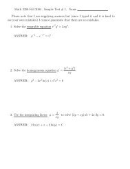
Example 6.3.9. The Tricomi Equation.<br />
u yy − yu xx =0.<br />
For this equation, D = b 2 − ac = y. So when y0<br />
the equation is hyperbolic and when y = 0 the equation is parabolic.<br />
For this example a = −y, b = 0 and c = 1 so the characteristic equation<br />
dy<br />
dx = b ± √ b 2 − ac<br />
a<br />
reduces to<br />
√<br />
dy −ac<br />
dx = ± a<br />
= ± 1 √ y<br />
.<br />
Since<br />
For y>0 the equation is hyperbolic and the characteristic curves are are given by<br />
3x ± 2y 3/2 = constant
6.3. CHARACTERISTICS AND HIGHER ORDER EQUATIONS 45<br />
The transformations<br />
ξ =3x − 2y 3/2 , η =3x +2y 3/2 ,<br />
reduce the equation to the normal form<br />
u ξη − 1 u ξ − u η<br />
6 ξ − η =0.<br />
y<br />
hyperbolic<br />
0<br />
elliptic<br />
Characteristics for Tricomi Equation<br />
x<br />
parabolic<br />
Return to Characteristics for Higher Order <strong>Equations</strong><br />
Let us return to the general notation for linear differential operators and characteristics<br />
introduced at the begining of the chapter. Namely, a kth order linear equation on Ω in R n<br />
is given by<br />
L = ∑<br />
a α (x)∂ α .<br />
|α|≤k<br />
The principal part of the equation is consists of all kth order terms<br />
P = ∑<br />
a α (x)∂ α .<br />
|α|=k<br />
Let us consider some examples For the Laplacian in two variables we have equation and<br />
principal part are the same and given by<br />
L = P = ∂ (2,0)<br />
1 + ∂ (0,2)<br />
2 = ∂2<br />
+ ∂2<br />
.<br />
∂x 2 1 ∂x 2 2
46 CHAPTER 6. PARTIAL DIFFERENTIAL EQUATIONS<br />
For the wave equation in R 2 we again have the equation and principal part are the same<br />
L = P = ∂ (2,0)<br />
1 − ∂ (0,2)<br />
2 = ∂2<br />
− ∂2<br />
.<br />
∂x 2 1 ∂x 2 2<br />
For the heat operator in R 2 we have the equation and principal part which in this case<br />
are not the same<br />
L = ∂ (2,0)<br />
1 − ∂ (0,1)<br />
2 = ∂2<br />
−<br />
∂ ,<br />
∂x 2 1 ∂x 2<br />
and<br />
P = ∂ (2,0)<br />
1 = ∂2<br />
.<br />
∂x 2 1<br />
The characteristic form (or principal symbol) atx ∈ Ω is the homogeneous polynomial<br />
of degree k defined for ξ ∈ R n by<br />
χ L (x, ξ) = ∑<br />
a α (x)ξ α .<br />
|α|=k<br />
A vector ξ is characteristic or is called a characteristic direction, for L at x if<br />
χ L (x, ξ) =0.<br />
The characteristic variety is the set of all characteristic vectors ξ, i.e.,<br />
Char x (L) ={ξ ≠0:χ L (x, ξ) =0}.<br />
As we already have defined, a surface (or curve) S is said to be characteristic with respect<br />
to L at x 0 if the normal vector ν(x 0 )atx 0 defines a characteristic directions.<br />
Example 6.3.10. Consider<br />
L = a(x, y) ∂<br />
∂x + b(x, y) ∂ ∂y = a (1,0)∂ (1,0) + a (0,1) ∂ (0,1) .<br />
The characteristic form is<br />
χ L (x, ξ) =a(x, y)ξ 1 + b(x, y)ξ 2 .<br />
Let C be a characteristic curve given parametrically by (x(t),y(t)). The tangent to this<br />
curve is (x ′ (t),y ′ (t)) and the normal is (y ′ (t), −x ′ (t)). Since C is a characteristic curve we<br />
must have<br />
a(x(t),y(t))y ′ (t) − b(x(t),y(t))x ′ (t) =0.<br />
Thus the characteristic curve can be found from<br />
dx<br />
dt = a(x(t),y(t)), dy<br />
dt = b(x(t),y(t))<br />
just as we defined them earlier.
6.3. CHARACTERISTICS AND HIGHER ORDER EQUATIONS 47<br />
Example 6.3.11. Reconsider the wave equation in R 2<br />
Lu = ∂ (2,0)<br />
1 u − ∂ (0,2)<br />
2 u = ∂2 u<br />
− ∂2 u<br />
=0.<br />
∂x 2 1 ∂x 2 2<br />
If ξ =(ξ 1 ,ξ 2 ) defines a characteristic direction, then we must have<br />
ξ 2 1 − ξ 2 2 =0.<br />
Now if C : (x(t),y(t)) is a characteristic curve, let<br />
ξ 1 = dy<br />
dt ,<br />
ξ 2 = − dx<br />
dt<br />
denote a normal to C. Then we have<br />
( ) 2 ( ) 2 ( dy dx dy<br />
− =<br />
dt dt dt − dx )( dy<br />
dt dt + dx )<br />
=0<br />
dt<br />
This equation is satisfied if we take<br />
or<br />
dy<br />
dx = ±1,<br />
y − x = c, y + x = c,<br />
and we see that the characteristic curves are straight lines (just as we saw earlier).<br />
Example 6.3.12. For the equation (6.3.4), the principal part is<br />
A characteristic curve (x(t),y(t)) has normal<br />
Pu = a ∂2 u<br />
∂x 2 +2b ∂2 u<br />
∂x∂y + c∂2 u<br />
∂y 2 .<br />
that satisfies<br />
or<br />
or<br />
a<br />
( ) 2 dy<br />
− 2b<br />
dt<br />
ξ 1 = dy<br />
dt ,<br />
ξ 2 = − dx<br />
dt<br />
aξ 2 1 +2bξ 1 ξ 2 + cξ 2 2 =0,<br />
( dy<br />
dt<br />
)( ) dx<br />
+ c<br />
dt<br />
ady 2 − 2bdydx + cdx 2 =0,<br />
( ) 2 dx<br />
=0,<br />
dt
48 CHAPTER 6. PARTIAL DIFFERENTIAL EQUATIONS<br />
or<br />
[ ( √ ) ][ ( √ ) ]<br />
b + b2 − ac<br />
b − b2 − ac<br />
a dy −<br />
dx dy −<br />
dx =0.<br />
a<br />
a<br />
Hence the characteristic curves can be found by solving<br />
( √ )<br />
dy b ±<br />
dx = b2 − ac<br />
,<br />
a<br />
just as we saw earlier.<br />
In an attempt to further illustrate the significance of characteristics consider the following<br />
example.<br />
Example 6.3.13. Consider the Cauchy problem that we looked at earlier<br />
Lu = ∂u<br />
∂x =0, u(x, 0) = f(x), (x, y) ∈ R2 .<br />
From the PDE we must have u(x, y) =F (y) and the initial condition gives u(x, 0) =<br />
f(x) =F (0) so that f must be a constant or the problem has no solution. If f(x) =c is a<br />
constant then we can take any F (y) such that F (0) = c so we get infinitely many solutions.<br />
Note that the characteristics for this example are determined by<br />
dy<br />
dx<br />
=0, ⇒ y = constant.<br />
So we have prescribed our initial data along a characteristic curve. Note that y is constant<br />
on a characteristic.<br />
6.3.2 The Cauchy Problem for Higher Order <strong>Equations</strong><br />
Let S be a hypersurface of class C k .Ifu ∈ C k−1 defined near S, then the Cauchy data of u<br />
on S is the set<br />
{u, ∂ ν u, ··· ,∂ν<br />
k−1 u}.<br />
We observe that we can consider the so-called Cauchy problem in a neighborhood of a<br />
single point and then introduced a change of variables to transform the problem so that S<br />
contains the origin and near the origin S coincides with the hyperplane x n =0. Thusit<br />
is often the case when treating higher order initial value problems that we distinguish the<br />
variable x n and denote it by t and then define x =(x 1 , ··· ,x n−1 ) ∈ R n−1 . Also we then<br />
consider ∂ t and ∂ x and multi-indices α =(α 1 , ··· ,α n−1 ). With this the Cauchy Problem is:
6.3. CHARACTERISTICS AND HIGHER ORDER EQUATIONS 49<br />
Given functions {φ j (x)} k−1<br />
j=0 solve<br />
F ( x, t, (∂ α x ∂ j t u) |α|+j≤k<br />
)<br />
=0<br />
with<br />
∂ j t u(x, 0) = φ j (x), 0 ≤ j ≤ (k − 1).<br />
This problem is far to general since the Cauchy data determine many derivatives on S.<br />
Indeed, up to order k the only unknown is ∂t k u. For the Cauchy problem to be well-posed it<br />
must be assumed that F = 0 can be solved for ∂t k . This is a characteristic condition on S.<br />
Numerous examples were given to illustrate this situation.<br />
We could embark on an in-depth treatment of the Quasi-linear case. In particular, we<br />
could consider the notion of noncharacteristic surface for the Cauchy problem: An initial<br />
value problem<br />
∑ ( )<br />
a α,j x, t, ((∂<br />
β<br />
x ∂tu) i |β|+i≤k−1 ∂<br />
α<br />
x ∂ j t u = b ( )<br />
x, t, (∂x β ∂tu) i |β|+i≤k−1<br />
|α|+j=k<br />
∂ j t u(x, 0) = φ j (x), 0 ≤ j ≤ (k − 1)<br />
is called non-characteristic if<br />
a 0,k<br />
(<br />
x, 0, (∂<br />
α<br />
x ∂ j t u) |α|+j≤k<br />
)<br />
≠0<br />
With this we could be in a position to prove the main fundamental existence and uniqueness<br />
result (such as it is) for PDE’s with analytic data. Rather that take such a deep<br />
excursion we will simple state the main result – the Cauchy-Kovalevski Theorem.<br />
Theorem 6.3.14. If G, {φ j } k−1<br />
j=0 are analytic near the origin, the Cauchy problem<br />
⎧ (<br />
)<br />
⎨ ∂t k u = G x, t, (∂x α ∂ j t u) |α|+j≤k<br />
j
50 CHAPTER 6. PARTIAL DIFFERENTIAL EQUATIONS<br />
Theorem 6.3.15. Suppose that a α , f, ϕ 1 , ··· ,ϕ k and the surface S are analytic (note that<br />
to say S is analytic means that if S is given by F (x 1 , ··· ,x n )=0then F is an analytic<br />
function). Suppose further that the initial surface S is not characteristic at x 0 ∈ S, i.e.,<br />
∑<br />
a α (x 0 ) [ ν(x 0 ) ] α<br />
≠0,<br />
|α|≤k<br />
where ν(x 0 ) is the normal to S at x 0 . Then the Cauchy problem has a solution u(x) in a<br />
neighborhood of x 0 . This solution is unique in the class of analytic solutions.<br />
Remark 6.3.16. 1. The Cauchy-Kovalevski theorem says that under certain conditions<br />
we can seek a solution in the form of a power series. While sometimes useful, this is<br />
not a very practical method of solution.<br />
2. The Cauchy-Kovalevski theorem guarantees that the Cauchy problem<br />
∆u(x, y) =0, |x| < ∞, y > 0,<br />
u(x, 0) = f(x), |x| < ∞,<br />
∂u<br />
(x, 0) = g(x), |x| < ∞<br />
∂x<br />
has a unique solution for every analytic f and g. It does not, however, say that the<br />
problem is well posed. Recall the Hadamard example we discussed earlier.<br />
At this point we mention that there are numerous related topics that should be considered<br />
if we had the time.<br />
Additional topics in this area include<br />
1. Holmgren uniqueness theorem<br />
2. Non-continuous dependence example of Hadamard<br />
3. Classical Lewy example of an equation with no solution of class C 1 for any C ∞ (not<br />
analytic) right hand side<br />
4. Malgrange-Ehrenpreis theorem on local solvability for constant coefficient operators.<br />
Unfortunately, with our time constraints the best we can do is to state some of these<br />
results for completeness.<br />
The first is the Holgren Uniqueness Theorem which says that analyticity is not required<br />
in the Cauchy-Kovalevski theorem to guarantee uniqueness.<br />
Theorem 6.3.17 (Holmgren’s Uniqueness Theorem). Under the same assumptions as<br />
the Cauchy-Kovalevski theorem, any two C k solutions in a neighborhood of x 0 must coincide<br />
in a perhaps smaller neighborhood of x 0 .
6.3. CHARACTERISTICS AND HIGHER ORDER EQUATIONS 51<br />
The next theorem due to Malgrange and Ehrenpreis gives an existence theorem for general<br />
constant coefficient equations.<br />
Theorem 6.3.18 (Malgrange-Ehrenpreis Theorem). If<br />
L = ∑<br />
a α ∂ α ,<br />
|α|≤k<br />
is a kth order linear differential equation with constant coefficients on R n and f ∈<br />
C0 ∞ (R n ) (the space of infinitely differentiable functions with compact support), then there<br />
exists a u ∈ C ∞ (R n ) such that Lu = f.<br />
On the flip side we should also mention the classical nonexistence example due to Hans<br />
Lewy (1957). This result shattered all hopes of generalizing the Cauchy-Kovalevski theorem<br />
to the non-analytic case.<br />
Consider the differential operator L defined in R 3 with coordinates (x, y, t) given by<br />
L = ∂<br />
∂x + i ∂ ∂y − 2i(x + iy) ∂ ∂t .<br />
Theorem 6.3.19 (Hans Lewy Theorem). Let f be a continuous real-valued function depending<br />
only on t. If there is a C 1 function u of (x, y, t) satisfying Lu = f in some neighborhood<br />
of the origin, then f must actually be analytic.<br />
Once this result is known, it is possible to show that there are C ∞ functions g on R 3<br />
such that the equation Lu = g has no solution u ∈ C 1+α (α>0) in any neighborhood of<br />
any point.
52 CHAPTER 6. PARTIAL DIFFERENTIAL EQUATIONS<br />
Exercise Set 2: Classification and Canonical Forms<br />
1. Classify the operators and find the characteristics (if any) through the point (0, 1):<br />
(a) u tt + u xt + u xx =0<br />
(b) u tt +4u xt +4u xx =0<br />
(c) u tt − 4u xt + u xx =0<br />
2. Find where the operators are hyperbolic, parabolic and elliptic:<br />
(a) Lu = u tt + tu xx + xu x<br />
(b) Lu = x 2 u tt − u xx + u<br />
(c) Lu = tu tt +2u xt + xu xx + u x<br />
3. Transform the equation to canonical form: 2u xx − 4u xy − 6u yy + u x =0.<br />
4. Transform the equations to canonical form:<br />
(a) e 2x u xx +2e x+y u xy + e 2y u yy + u x =0.<br />
(b) x 2 u xx + y 2 u yy = 0 for x>0, y>0.<br />
5. Transform the equations to canonical form:<br />
(a) u xx +2u xy +17u yy =0.<br />
(b) 4u xx +12u xy +9u yy − 2u x + u =0.<br />
6. Find the characteristics of Lu = u tt − tu xx through the point (0, 1).<br />
7. Determine where the following equation is hyperbolic or parabolic.<br />
yu xx +(x + y)u xy + xu yy =0<br />
Where the equation is hyperbolic, show that the general solution may be written as<br />
u(x, y) = 1 ∫<br />
f(β) dβ + g(y − x).<br />
y − x<br />
where β = y 2 − x 2<br />
8. Classify the following equation and find the canonical form, u xx − 2u xt + u tt =0. Show<br />
that the general solution is given by u(x, t) =tf(x + t)+g(x + t).<br />
9. Show that (1 + x 2 )u xx +(1+y 2 )u yy + xu x + yu y = 0 is elliptic and find the canonical<br />
form of the equation.
Bibliography<br />
[1] R. Dautray and J.L. Lions, Mathematical analysis and numerical methods for science<br />
and technology,<br />
[2] G. Folland, Introduction to partial differential equations,<br />
[3] A. Friedman, Generalized functions and partial differential equations,<br />
[4] A. Friedman, <strong>Partial</strong> differential equations,<br />
[5] K.E. Gustafson <strong>Partial</strong> differential equations,<br />
[6] P.R. Garabedian, <strong>Partial</strong> <strong>Differential</strong> <strong>Equations</strong>, New York, John Wiley & Sons, 1964.<br />
[7] I.M. Gel’fand and G.E. Shilov, Generalized functions, v. 1,<br />
[8] G. Hellwig, <strong>Partial</strong> differential equations, New York, Blaisdell Publ. Co. 1964.<br />
[9] L. Hörmander, Linear partial differential operators,<br />
[10] F. John, <strong>Partial</strong> differential equations,<br />
[11] J. Kevorkian, <strong>Partial</strong> differential equations,<br />
[12] P. Lax, Hyperbolic systems of conservation laws and the mathematical theory of shocks,<br />
[13] I.G. Petrovsky, Lectures on partial differential equations, Philadelphia, W.B. Saunders<br />
Co. 1967.<br />
[14] M. Pinsky, Introduction to partial differential equations with applications,<br />
[15] W. Rudin, Functional analysis,<br />
[16] F. Treves, Basic <strong>Partial</strong> <strong>Differential</strong> <strong>Equations</strong>, New York, Academic Press, 1975.<br />
[17] F. Treves, Linear <strong>Partial</strong> <strong>Differential</strong> <strong>Equations</strong> with Constant Coefficients, New York,<br />
Gordon & Breach, 1966.<br />
53
54 BIBLIOGRAPHY<br />
[18] K. Yosida, Functional analysis,<br />
[19] Generalized functions in mathematical physics, V.S. Vladimirov<br />
[20] H.F. Weinberger, <strong>Partial</strong> differential equations, Waltham, Mass., Blaisdel Publ. Co.,<br />
1965.<br />
[21] E.C. Zachmanoglou and D.W. Thoe, Introduction to partial differential equations with<br />
applications,<br />
[22] A.H. Zemanian, Distribution theory and transform analysis,