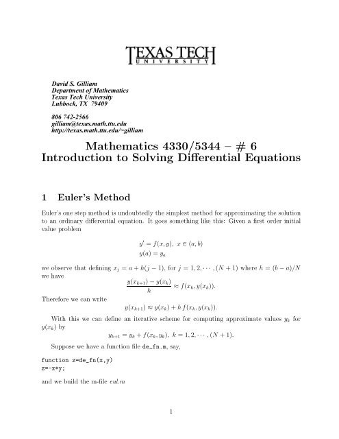
Matlab Lesson 6 for Math 4330 and 5344 - Texas Tech University

David S. Gilliam
Department of Mathematics
Texas Tech University
Lubbock, TX 79409
806 742-2566
gilliam@texas.math.ttu.edu
http://texas.math.ttu.edu/~gilliam
Mathematics 4330/5344 –#6
Introduction to Solving Differential Equations
1 Euler’s Method
Euler’s one step method is undoubtedly the simplest method for approximating the solution
to an ordinary differential equation. It goes something like this: Given a first order initial
value problem
y ′ = f(x, y), x∈ (a, b)
y(a) =y a
we observe that defining x j = a + h(j − 1), for j =1, 2, ··· , (N + 1) where h =(b − a)/N
we have
y(x k+1 ) − y(x k )
≈ f(x k ,y(x k )).
h
Therefore we can write
y(x k+1 ) ≈ y(x k )+hf(x k ,y(x k )).
With this we can define an iterative scheme for computing approximate values y k for
y(x k )by
y k+1 = y k + f(x k ,y k ),k=1, 2, ··· , (N +1).
Suppose we have a function file de_fn.m, say,
function z=de_fn(x,y)
z=-x*y;
and we build the m-file eul.m
1

clear
% this program calls the function file de_fn.m
a=input(’left end point a = ’);
b=input(’right end point b = ’);
N=input(’ number of sub-intervals, N = ’);
ya=input(’initial value at x=a, ya= ’);
h=(b-a)/N;
x=a+h*(1:(N+1));
lx=length(x);
y(1)=ya;
for j=1:N
y(j+1)=y(j)+h*f(x(j),y(j));
end
plot(x,y)
This method can also be applied to higher dimensional problems as demonstrated in the
following example. Consider the second order initial value problem
y ′′ = f(x, y, y ′ ), x ∈ [a, b]
y(a) =y a
y ′ (a) =y pa
If we set w = y and z = y ′ , then the system can be written as
[ ] [ ]
d w z
=
dx z f(x, w, z)
w(a) =y a
z(a) =y pa
The numerical approximation can now be carrried out just as above. Suppose we have a
function file de2_fn.m, say,
function z=de2_fn(x,y,yp)
z=-x*y/(yp^2+1);
Now we build an m-file eul2.m to solve the problem.
clear
% this program calls the function file de2_fn.m
a=input(’left end point a = ’);
b=input(’right end point b = ’);
N=input(’ number of sub-intervals, N = ’);
ya=input(’initial value at x=a, y(a)= ’);
yap=input(’initial value at x=a, y’’(a)= ’);
h=(b-a)/N;
2

x=a+h*(1:(N+1));
lx=length(x);
w(1)=ya;
z(1)=ypa;
for j=1:N
w(j+1)=w(j)+h*z(j);
z(j+1)=z(j)+h*de2_fn(x(j),w(j),z(j));
end
y=w;
plot(x,y)
There are many variations on the Euler method. Some of them are given in the first
exercise in this lesson.
2 Matlab Builtin ODE Solvers
In addition there are many other methods for approximating solutions to ordinary differential
equations, but due to a lack of time left in the semester I will just introduce you to Matlabs
builtin Runge-Kutta solver ode45 and show you how it works. I will also give you a copy
of a more recent version of the ode45 solver which comes from a collection of files in the
ode suite which were written by researchers at SMU in Dallas. This new version is now the
standard version in the newest Matlab version 5.
Here is the help file for the solver in your current version of Matlab.
ODE45 Solve differential equations, higher order method.
ODE45 integrates a system of ordinary differential equations using
4th and 5th order Runge-Kutta formulas.
[T,Y] = ODE45(’yprime’, T0, Tfinal, Y0) integrates the system of
ordinary differential equations described by the M-file YPRIME.M,
over the interval T0 to Tfinal, with initial conditions Y0.
[T, Y] = ODE45(F, T0, Tfinal, Y0, TOL, 1) uses tolerance TOL
and displays status while the integration proceeds.
INPUT:
F - String containing name of user-supplied problem description.
Call: yprime = fun(t,y) where F = ’fun’.
t - Time (scalar).
y - Solution column-vector.
yprime - Returned derivative column-vector; yprime(i) = dy(i)/dt.
t0 - Initial value of t.
tfinal- Final value of t.
y0 - Initial value column-vector.
tol - The desired accuracy. (Default: tol = 1.e-6).
trace - If nonzero, each step is printed. (Default: trace = 0).
3

OUTPUT:
T - Returned integration time points (column-vector).
Y - Returned solution, one solution column-vector per tout-value.
The result can be displayed by: plot(tout, yout).
You should compare this with the help file from the new ode45.m solver from the ode
suite.
ODE45 Solve non-stiff differential equations, medium order method.
[T,Y] = ODE45(’ydot’,TSPAN,Y0) with TSPAN = [T0 TFINAL] integrates
the system of first order differential equations y’ = ydot(t,y) from
time T0 to TFINAL with initial conditions Y0. Function ydot(t,y)
must return a column vector. Each row in solution matrix Y
corresponds to a time returned in column vector T. To obtain
solutions at the specific times T0, T1, ..., TFINAL (all increasing
or all decreasing), use TSPAN = [T0 T1 ... TFINAL].
[T,Y] = ODE45(’ydot’,TSPAN,Y0,OPTIONS) solves as above with default
integration parameters replaced by values in OPTIONS, an argument
created with the ODESET function. See ODESET for details. Commonly
used options are scalar relative error tolerance ’rtol’ (1e-3 by
default) and vector of absolute error tolerances ’atol’ (all
components 1e-6 by default).
It is possible to specify tspan, y0 and options in ydot. If TSPAN
or Y0 is empty, or if ODE45 is invoked as ODE45(’ydot’), ODE45 calls
[tspan,y0,options] = ydot([],[]) to obtain any values not supplied
at the command line.
As an example, the commands
options = odeset(’rtol’,1e-4,’atol’,[1e-4 1e-4 1e-5]);
ode45(’rigid’,[0 12],[0 1 1],options);
solve the system y’ = rigid(t,y) with relative error tolerance 1e-4
and absolute tolerances of 1e-4 for the first two components and
1e-5 for the third. When called with no output arguments, as in
this example, ODE45 calls the default output function ODEPLOT to
plot the solution as it is computed.
Lets look at a couple of other examples. One version of the van der Pohl oscillator is
given by the following second order initial value problem on an interval (0,T), for T>0.
4

d 2 z
dt + 2 µ(z2 − 1) dz
dt + z =0
dz
z(0) = z 0 ,
dt (0) = z 1
We transform this problem to a first order system by introducing y 1 = z and y 2 = dz
[ ]
dt
y1
and defining y = . With this we can write
y 2
[ ]
d y1
dt y 2
y(0) =
[
=
]
z 1
[
z0
]
y 2
µ(1 − y1)y 2 2 − y 1
To solve this problem numerically we build a function file named vdpde.m
function yp = vdpde(t,y)
global MU
yp(1)=y(2);
yp(2)=MU*y(2).*(1-y(1).^2)-y(1);
Now we build an m-file run_vdp.m to setup and run the problem. In this case I am going
to use the new ode45.m routine from the ode suite. When you run the program you can pick
various values of MU. You might start with MU=1. As you change this value, you will notice
that the “limit cycle” can change considerably. Run the problem for several different initial
conditions for the same MU and you will see why we speak of a limit cycle.
clear
clear global
global MU
t0=input(’ initial time t0 = ’);
T=input(’ final time T = ’);
MU=input(’ parameter MU = ’);
v=input(’ vector of initial conditions v = [v1,v2] ’);
[n,m]=size(v);
if m>1
v=v’;
end
tvec=t0:.025:T;
[t,y]=ode45(’vdpde’,tvec,v);
plot(y(:,1),y(:,2))
5

As another example consider the famous Lorenz equations whose solution exhibits the
so-called lorenz attractor.
dy 1
dt = 10(y 2 − y 1 );
dy 2
dt = (28 − y 3)y 1 − y 2 ;
dy 3
dt = y 1y 2 − (8/3)y 3 ;
Build a function file lorenzde.m
function dy=lorenzde(t,y)
dy=[10*(y(2)-y(1)); (28-y(3)).*y(1)-y(2); y(1).*y(2)-(8/3)*y(3)];
clear
Now build a file run_lorenz.m to run the problem
t0=input(’ initial time t0 = ’);
T=input(’ final time T = ’);
% initial condition; e.g. [1 -1 2]’
v=input(’ vector of initial conditions v = [v1,v2,v3] ’);
[n,m]=size(v);
if m>1
v=v’;
end
tvec=t0:.025:T;
[t,y]=ode45(’lorenzde’,tvec,v);
h1=figure
plot(y(:,1),y(:,2))
h2=figure
plot(y(:,1),y(:,3))
h3=figure
plot(y(:,2),y(:,3))
ASSIGNMENT 6 – Math 4330 and 5344
1. This problem is concerned with several variations on the Euler’s method. I want you
to modify your Euler program by adding each of these methods and then compare
the resulting accuracy by finding the maximum of the absolute value of the difference
of the solution for each method and the exact solution on a vector of x values
x=linspace(a,b). Make a table to print out the results.
6

(a) Euler y 1 = ya, y j+1 = y j + hf(x j ,y j )
(b) Midpoint y 1 = ya, y j+1 = y j + hf ( x j + h 2 ,y j + h 2 f(x j,y j ) )
(c) Modified Euler y 1 = ya, y j+1 = y j + h [
f(xj ,y j )+f(x j ,y j + hf(x j ,y j )) ]
2
(d) Huen y 1 = ya, y j+1 = y j + h [
f(xj ,y j )+3f(x j + 2h 4
3 ,y j + 2h 3 f(x j,y j )) ]
For this comparison take N = 50 and 100 and apply to the follwing differential equations:
(a) y ′ = −y + x +1, 0 ≤ x ≤ 1, y(0) = 1, exact: y = x + e −x
(b) y ′ = y + x, 0 ≤ x ≤ 2, y(0) = −1, exact: y = −x − 1
(c) y ′ = x −2 − x −1 y, 1 ≤ x ≤ 2, y(1) = −1, exact: y = log(x) − 1 x x
(d) y ′ = y − xy 3 e −2x , 0 ≤ x ≤ 1, y(0) = 1, exact: y =(x 2 +1) −1/2 e x
In the table, include a column giving the values of h =(b − a)/N .
2. Use ode45.m to solve the harmonic oscillator problem
d
dt y 1 =2y 2
d
dt y 2 = −2y 1
y 1 (0)=0,
y 2 (0)=1
Plot (y 1 ,y 2 ), (t, y 1 ) and (t, y 2 ).
I would use t0 =0andT =4π with t = linspace(t0,T,300).
7