Matlab Lesson 6 for Math 4330 and 5344 - Texas Tech University
Matlab Lesson 6 for Math 4330 and 5344 - Texas Tech University
Matlab Lesson 6 for Math 4330 and 5344 - Texas Tech University

Create successful ePaper yourself
Turn your PDF publications into a flip-book with our unique Google optimized e-Paper software.
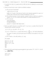
clear<br />
% this program calls the function file de_fn.m<br />
a=input(’left end point a = ’);<br />
b=input(’right end point b = ’);<br />
N=input(’ number of sub-intervals, N = ’);<br />
ya=input(’initial value at x=a, ya= ’);<br />
h=(b-a)/N;<br />
x=a+h*(1:(N+1));<br />
lx=length(x);<br />
y(1)=ya;<br />
<strong>for</strong> j=1:N<br />
y(j+1)=y(j)+h*f(x(j),y(j));<br />
end<br />
plot(x,y)<br />
This method can also be applied to higher dimensional problems as demonstrated in the<br />
following example. Consider the second order initial value problem<br />
y ′′ = f(x, y, y ′ ), x ∈ [a, b]<br />
y(a) =y a<br />
y ′ (a) =y pa<br />
If we set w = y <strong>and</strong> z = y ′ , then the system can be written as<br />
[ ] [ ]<br />
d w z<br />
=<br />
dx z f(x, w, z)<br />
w(a) =y a<br />
z(a) =y pa<br />
The numerical approximation can now be carrried out just as above. Suppose we have a<br />
function file de2_fn.m, say,<br />
function z=de2_fn(x,y,yp)<br />
z=-x*y/(yp^2+1);<br />
Now we build an m-file eul2.m to solve the problem.<br />
clear<br />
% this program calls the function file de2_fn.m<br />
a=input(’left end point a = ’);<br />
b=input(’right end point b = ’);<br />
N=input(’ number of sub-intervals, N = ’);<br />
ya=input(’initial value at x=a, y(a)= ’);<br />
yap=input(’initial value at x=a, y’’(a)= ’);<br />
h=(b-a)/N;<br />
2