Chapter 6 Partial Differential Equations

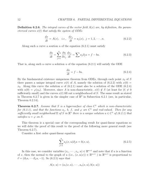
12 CHAPTER 6. PARTIAL DIFFERENTIAL EQUATIONS
Definition 6.2.6. The integral curves of the vector field A(x) are, by definition, the parameterized
curves x(t) that satisfy the system of ODEs
dx
dt = A(x), i.e., dx j
dt = a j(x), j =1, 2, ··· ,n. (6.2.2)
Along such a curve a soution u of the equation (6.2.1) must satisfy
du
dt =
n∑
j=1
∂u
∂x j
dx j
dt = ∑ a j ∂ j u = f − bu. (6.2.3)
That is, along such a curve a solution u of the equation (6.2.1) will satisfy the ODE
du
= f − bu. (6.2.4)
dt
By the fundamental existence uniqueness theorem from ODEs, through each point x 0 of S
there passes a unique integral curve x(t) ofA, namely the solution of (6.2.2) with x(0) =
x 0 . Along this curve the solution u of (6.2.1) must also be a solution of the ODE (6.2.4)
with u(0) = ϕ(x 0 ). Moreover, since A is non-characteristic, x(t) ∉ S (at least for |t| ≠0
sufficiently small) and the curves x(t) fill out a neighborhood of S. The same result as stated
in Theorem 6.2.7 is given in the simpler case of R 2 in Subsection 6.2.1 (see, in particular,
Theorem 6.2.14).
Theorem 6.2.7. Assume that S is a hypersurface of class C 1 which is non-characteristic
for (6.2.1), and that the functions a j , b, f, and ϕ are C 1 and real-valued. Then for any
sufficiently small neighborhood Ω of S in R n there is a unique solution u ∈ C 1 of (6.2.1) that
satisfies u = ϕ on S.
This theorem is a special case of the corresponding result for quasi-linear equations so
we will defer the proof of this result to the proof of the following more general result (see
Theorem 6.2.7).
Consider a first order quasi-linear equation
n∑
a j (x, u)∂ j u = b(x, u). (6.2.5)
j=1
In this case, we consider variables (x 1 , ··· ,x n ,u) ∈ R n+1 and note that if u is a function
of x, then the normal to the graph of u (i.e., (x, u(x)) ∈ R n+1 )inR n+1 is proportional to
⃗v =(∂ 1 u, ···∂ n u, −1). So (6.2.5) says that
A(x, u) =(a 1 (x, u), ··· ,a n (x, u),b(x, u))