Chapter 6 Partial Differential Equations

6.2. LINEAR AND QUASILINEAR EQUATIONS OF FIRST ORDER 17
6.2.1 Special Case: Quasilinear Equations in R 2
As a special case let us consider n = 2, i.e., let us consider first order quasi-linear (or linear)
equations in two variables in the form
a(x, y, u) ∂u + b(x, y, u)∂u
∂x ∂y
= c(x, y, u). (6.2.9)
For this example we adhere to common practice and refer to the variables as x and y or x
and t, depending on the given problem, instead of x 1 and x 2 . Also in this case it is often
useful to use the notations
u x = ∂u
∂x ,u y = ∂u
∂y ,u t = ∂u
∂t , etc.
for the various partial derivatives.
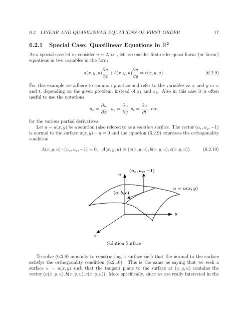
Let u = u(x, y) be a solution (also refered to as a solution surface. The vector (u x ,u y , −1)
is normal to the surface u(x, y) − u = 0 and the equation (6.2.9) expresses the orthogonality
condition
A(x, y, u) · (u x ,u y , −1)=0, A(x, y, u) ≡ (a(x, y, u),b(x, y, u),c(x, y, u)). (6.2.10)
u
(u x ,u y , −1)
(a, b, c)
u = u(x, y)
y
x
Solution Surface
To solve (6.2.9) amounts to constructing a surface such that the normal to the surface
satisfys the orthogonality condition (6.2.10). This is the same as saying that we seek a
surface u = u(x, y) such that the tangent plane to the surface at (x, y, u) contains the
vector (a(x, y, u),b(x, y, u),c(x, y, u)). More specifically, since we are really interested in the