Simplified recursive algorithm for Wigner 3j and 6j symbols - iucaa

PHYSICAL REVIEW E VOLUME 57, NUMBER 6
JUNE 1998
Simplified recursive algorithm for Wigner 3j and 6j symbols
James H. Luscombe
Department of Physics, Naval Postgraduate School, Monterey, California 93943
Marshall Luban
Ames Laboratory and Department of Physics and Astronomy, Iowa State University, Ames, Iowa 50011
Received 8 January 1998
We present a highly accurate, ab initio recursive algorithm for evaluating the Wigner 3 j and 6 j symbols.
Our method makes use of two-term, nonlinear recurrence relations that are obtained from the standard threeterm
recurrence relations satisfied by these quantities. The use of two-term recurrence relations eliminates the
need for rescaling of iterates to control numerical overflows and thereby simplifies the widely used recursive
algorithm of Schulten and Gordon. S1063-651X9802506-9
PACS numbers: 02.70.c, 31.15.p, 03.65.w
The Wigner 3 j and 6 j symbols arise frequently in contexts
involving the coupling of angular momenta in quantum
mechanics and other applications of the rotation group.
While one can utilize the explicit expressions of Wigner 1
and Racah 1 to calculate specific values of these quantities,
computationally the direct approach is often impractical, especially
for large quantum numbers. As has long been recognized,
a convenient alternative numerical approach is to
make use of the three-term recurrence relations see Eq. 1
satisfied by these quantities. In 1975, Schulten and Gordon
SG 2developed an ab initio recursive algorithm that has
come to be widely used. A particular advantage of the SG
method is that it produces, as the result of the same calculation,
not just the value of a single 3 j or 6 j symbol, as is the
case with the direct approach, but values for an entire family
of symbols whereby one quantum number is allowed to
range over its allowed values with the other parameters of
the symbol held fixed. From a computational point of view,
however, a limitation of the SG method is that it readily
leads to numerical overflows. Existing implementations of
the SG method are designed to test for the occurrence of
overflows and periodically rescale the iterates so as to keep
them of a manageable magnitude to ensure numerical accuracy.
The purpose of this article concerns the limitation of the
SG recursive method: overflows and the need for countermeasures.
We show that this feature can be avoided entirely.
Now, each of the 3 j or 6 j symbols f ( j), g(m), or h(j),
listed in Table I, separately obeys a recurrence relation of the
form
X nn1Y nnZ nn10,
n min nn max ,
where (n) signifies either f ( j), g(m), or h(j), with the
index n denoting j or m together with its allowed range of
values, n min nn max . We also list in Table I the functions
X , Y , and Z that appear in the recurrence relation for
each symbol, as well as the minimum and maximum values
of the variable j or m. We propose to solve Eq. 1, a linear,
three-term recurrence relation, by working with a pair of
1
nonlinear, two-term recurrence relations, each equivalent to
Eq. 1, which are defined in terms of the ratios of successive
values of (n). The first is given in terms of the ratios
r (n)(n)/(n1),
Z n
r n
Y nX nr n1 , nn max1. 2
Note that Eq. 2 defines a backwards recurrence scheme,
where, since X (n max 1)0 for each of the symbols in
Table I, the starting value r (n max )Z (n max )/Y (n max )is
known. As an example, the version of Eq. 2 associated with
the 3 j symbol f ( j) is, using the information in Table I, given
by r f ( j)(j1)A(j)/B(j)jA(j1)r f (j1). The
second recurrence relation is defined in terms of the ratios
s (n)(n)/(n1), which are suitable for forward iteration.
In terms of these quantities, Eq. 1 is equivalent to
X n
s n
Y nZ ns n1 , nn min1, 3
where, since Z (n min )0, the starting value is known,
s (n min )X (n min )/Y (n min ). The numerical advantage of
making such transformations on Eq. 1 is that r (n) and
s (n) maintain values of order unity throughout the iteration,
which eliminates the possibility of overflows. The reason
for considering separate backward and forward iteration
schemes pertains to issues of numerical stability that are discussed
below. Before delving into these issues, however, it
will be instructive to illustrate the use of Eqs. 2 and 3.
We illustrate the use of Eqs. 2 and 3 upon assuming
that the (n) remain nonzero throughout the allowed range.
We first employ a backward iteration on Eq. 2 from n
n max down to nn mid 1, where n mid is some convenient
midpoint, e.g., n mid 1 2 (n min n max ). One will thus have generated
the sequence of iterates r (n max ),r (n max
1),...,r (n mid 1). It is then straightforward to obtain (n)
for n mid 1nn max ,
n mid kn mid r n mid p,
p1
k
1063-651X/98/576/72744/$15.00 57 7274 © 1998 The American Physical Society

57 SIMPLIFIED RECURSIVE ALGORITHM FOR WIGNER ...
7275
TABLE I. Parameters for, and constituents of, the three-term recurrence relations satisfied by the 3 j and 6 j symbols, as represented by
Eq. 1. In each case, all parameters except the variable j or m are held fixed. Also listed are the normalization condition and sign convention
for each symbol. We use the notation of Ref. 2.
3 j or 6 j
symbol
fj
j j 2 j 3
m 2 m 3 m 2
m 3
gm j 1
j 2
m 1 m
j 3
mm 1
hj j
l 1
j 2
l 2
j 3
l 3
Variable j m j
X jA(j1) C(m1) jE(j1)
Y B(j) D(m) F(j)
Z (j1)A(j) C(m) (j1)E(j)
Ajj 2 j 2 j 3 2 j 2 j 3 1 2 j 2
Cmj 2 m1j 2 m
E j j 2 j 2 j 3 2
j 2 m 2 m 3 2 1/2
j 3 mm 1 1
j 2 j 3 1 2 j 2
j 3 mm 1 1/2
j 2 l 2 l 3 2
Functions
B j2 j1m 2 m 3
Dmj 2 j 2 1j 3 j 3 1
l 2 l 3 1 2 j 2 1/2
Fj2j1jj1jj1
j 2 j 2 1j 3 j 3 1
j 1 j 1 1
j 2 j 2 1j 3 j 3 1
m 2 m 3 jj1
2mmm 1
2l 1 l 1 1l 2 l 2 1
jj1j 2 j 2 1
j 3 j 3 1l 3 l 3 1
jj1j 2 j 2 1
j 3 j 3 1
End points j min max(j 2 j 3 ,m 2 m 3 ) m min max(j 2 ,j 3 m 1 ) j min max(j 2 j 3 ,l 2 l 3 )
j max j 2 j 3 m max min(j 2 ,j 3 m 1 ) j max min(j 2 j 3 ,l 2 l 3 )
Normalization
j
max
jjmin2j1f
2 m
j1 2j 1 1 max
mmming
2 m1 (2l 1 1) jjmin(2j1)h
2 (j)1
j max
Sign sgnf(j max )(1) j 2 j 3 m 2 m 3 sgng(m max )(1) j 2 j 3 m 1 sgnh(j max )(1) j 2 j 3 l 2 l 3
1kn max n mid .
Of course, the value of (n mid ) is presently unknown; it will
be determined shortly through normalization. We now iterate
Eq. 3 from nn min up to nn mid 1; this produces the
iterates s (n min ),s (n min 1),...,s (n mid 1). From these
quantities we obtain (n) for n min nn mid 1,
n mid kn mid s n mid p,
p1
1kn mid n min .
With the combined equations 4 and 5, we have thus determined
the (n) up to an unknown multiplicative factor
(n mid ). The magnitude of this factor is readily determined
by imposing the normalization conditions given in Table I.
We then utilize the phase information listed in Table I to
completely determine (n) for all n. As an example, we
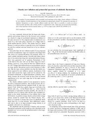
show in Fig. 1 the result of applying this simple algorithm to
obtain the family of 3 j symbols,
k
4
5
f j
j
15
100
70
60
,
55
which remains nonzero over the allowed range 40 j160.
The 3 j and 6 j symbols, of course, can and do vanish for
selected values of their parameters. If, say, (n 0 )0,
r (n 0 1) and s (n 0 1) are undefined. We must therefore
modify the above algorithm to account for this possibility,
and we will be guided by the following observations. Examining
Fig. 1, we note the resemblance between f ( j) and a
one-dimensional bound quantum eigenstate. This is a generic
feature of the 3 j and 6 j symbols; we use f ( j) merely as an
illustration. Now, it is known, from the semiclassical theory
of the 3 j and 6 j symbols 3, that the range of allowed
quantum numbers, n min nn max , can be divided into the
following subranges: a ‘‘classical’’ region n I nn II and
two complementary ‘‘nonclassical’’ regions n min nn I and
n II nn max . The classical region is defined as the set of
quantum numbers for which it is possible to construct a vector
diagram showing the coupling of the angular momentum
vectors; in the nonclassical regimes, such vector diagrams do
not exist 4. The limits of the classical region, n I and n II ,

7276 JAMES H. LUSCOMBE AND MARSHALL LUBAN
57
FIG. 1. Values for the family of 3 j symbols, f ( j)
j 100
( 15 70
60 55 ), over the entire range of allowed j values, 40 j
160. In the classical region, j I j j II , where here j I 49 and
j II 98 shown as dashed lines, f ( j) has an oscillatory character; in
the nonclassical regions, f ( j) decays monotonically. There are are
25 orders of magnitude difference between the largest and smallest
values in this family of 3 j symbols.
are determined as the roots of a certain determinant, known
as the Cayley determinant 3. For the parameters of Fig. 1,
these are shown as dashed lines. The important point is that,
in analogy with a bound eigenstate, in the classical region the
3 j and 6 j symbols have an oscillatory character, whereas in
the nonclassical regions, they are monotonically decaying
3. Depending on the width of the nonclassical regions,
there can be many orders of magnitude difference between
the smallest values of (n) found at n max and n min and
the largest values, which occur in the classical region. In Fig.
1, for example, there are some 25 orders of magnitude difference
between the largest and smallest values in this family
of 3 j symbols.
These considerations are relevant for the following reasons.
In numerical treatments of the one-dimensional Schrödinger
equation, one employs the standard finite-difference
approximation to replace the continuous differential equation
by a three-term recurrence relation. We note that, conversely,
as discussed in Ref. 2, the three-term recurrence relations
satisfied by the 3 j and 6 j symbols can be shown to originate
from eigenvalue problems. Now, as is well known, threeterm
recurrence relations possess two linearly independent
solutions. If the desired physical solution of a recurrence
relation is monotonically decreasing, as with the decay of
(n) in its nonclassical regions, it is simple to show that the
other, linearly independent solution will be monotonically
increasing. Indeed, the source of the numerical instability
associated with three-term recurrence relations is that 5 if
one attempts to calculate a decaying solution of the recurrence
relation by forward iteration, the slightest round-off
error will trigger the growth of the unwanted, linearly independent,
diverging solution.
Therefore, in the nonclassical regions one must iterate the
recurrence relation in the direction of increasing (n) to
avoid the instability. These are also just the regions where
overflows can develop. By contrast, in the classical region,
where the solutions to the recurrence relation are oscillatory,
there is no source of instability and one may safely iterate in
either direction. The problem we seek to avoid in our ratiobased
method is that of encountering an identically zero
value of . The zeros of , however, if they occur, occur
only in the classical region, where (n) is oscillatory. We
therefore adopt a hybrid approach. We utilize the two-term
recurrence relations 2 and 3 in the respective nonclassical
regions and the three-term recurrence relation 1 in the classical
region.
For our purposes, however, precisely where one draws the
line between the classical and nonclassical regions is not
crucial; all that is important is that we stop iterating with
Eqs. 2 and 3 somewhere in the classical region, before we
encounter a zero of (n). We will therefore adopt the following
convention. In iterating Eqs. 2 and 3, starting
from n max and n min , respectively, we note that both r (n)
and s (n) initially maintain values less than unity. Only
when we reach the first local extremum of (n) dor and s
first exceed unity. This provides a natural criterion for the
locations of the boundaries and one that is simple to implement
algorithmically. We will denote the values of n where
r (n) and s (n) first exceed unity having started from n max
and n min by n and n , respectively. Specifically, we have
r (n )1, but r (n 1)1.
The modifications of Eqs. 4 and 5 then become
and
n kn r n p,
p1
1kn max n ,
n kn s n p,
p1
1kn n min ,
k
k
4
5
where, as before, r and s are obtained from Eqs. 2 and
3, now for n nn max and n min nn , respectively. At
this point, we have the unknown quantities in Eqs. (4) and
(5), (n ) and (n ). We can eliminate one of these
unknowns in terms of the other as follows. Let us define two
auxiliary sequences (n)(n)/(n ) and (n)
(n)/(n ). These quantities obviously satisfy the same
three-term recurrence relation 1. One can then use Eq. 1
to iterate (n) in the forward direction starting from n
n , using the initial values (n 1)s (n 1) and
(n )1, up to some value of n, n c n , say. For convenience,
we can take n c n if desired. Likewise, we can
use Eq. 4 to iterate (n) in the backward direction starting
from nn , using the initial values (n 1)
r (n 1) and (n )1, down to nn c . The value of
(n c ) derived from these two sequences must obviously be
identical. This yields the connection between (n ) and
(n ), (n )/(n ) (n c )/ (n c ). Multiplying the
(n) which have now been evaluated unambiguously for
n min nn c by (n )/(n ) thus leaves us with (n)
for n min nn max ; i.e., we have determined (n) uptothe

57 SIMPLIFIED RECURSIVE ALGORITHM FOR WIGNER ...
7277
unknown multiplicative factor (n ). As before, we determine
this factor by applying the normalization conditions
and sign conventions given in Table I.
In conclusion, we have presented a recursive algorithm to
compute the Wigner 3 j and 6 j symbols that simplifies the
well-known SG method. Our method is based on the use of
nonlinear, two-term recurrence relations that are obtained
from the standard three-term recurrence relations obeyed by
the 3 j and 6 j symbols. By eliminating the programming
overhead of having to check for near overflows and keeping
track of rescaling factors, our algorithm provides a highly
accurate, yet significantly simpler framework, with which to
calculate these quantities.
ACKNOWLEDGMENTS
Ames Laboratory is operated for the U.S. Department of
Energy by Iowa State University under Contract No. W-
7405-Eng-82. We would like to acknowledge useful conversations
with Scott Davis, I. Y. Lee, Xavier Maruyama, Frank
Stevens, and Don Walters.
1 E. P. Wigner, Group Theory Academic Press, New York,
1959, p. 191; G. Racah, Phys. Rev. 62, 438 1942. A useful
summary of the 3 j and 6 j symbols and the Wigner-Racah
formulas is given by A. Messiah, Quantum Mechanics North-
Holland, Amsterdam, 1962, Vol. II, Appendix C.
2 K. Schulten and R. G. Gordon, J. Math. Phys. 16, 1961 1975.
While the various three-term recurrence relations satisfied by
the 3 j and 6 j symbols have been derived previously by several
authors, Schulten and Gordon provide a useful, unified derivation
of these recurrence relations.
3 Semiclassical approximations are discussed in detail by G.
Ponzano and T. Regge, in Spectroscopic and Group Theoretical
Methods in Physics, edited by F. Bloch et al. North-
Holland, Amsterdam, 1968, pp. 1–58. Additional semiclassical
results are derived by K. Schulten and R. G. Gordon, J.
Math. Phys. 16, 1971 1975. Early work on the classical limits
of the 3 j and 6 j symbols includes that of Wigner 1, Chap.
27, and P. J. Brussaard and H. A. Tolhoek, Physica Amsterdam
23, 955 1957.
4 For many quantum-mechanically allowed 3 j and 6 j symbols,
there do not exist vector diagrams showing the coupling of the
angular momentum vectors. For example, consider
2 j j j
( 0 j j); this is but one example of a well-defined 3 j symbol
of value (2 j)!/(4j1)! for which a vector addition
diagram does not exist for j 2. 1 The ‘‘classical region’’ of
the 3 j and 6 j symbols is defined as the set of quantum numbers
for which vector diagrams do exist.
5 See, for example, the discussion given by M. Luban and J. H.
Luscombe, Phys. Rev. B 35, 9045 1987 and by W. H. Press,
S. A. Teukolsky, W. T. Vetterling, and B. P. Flannery, Numerical
Recipes Cambridge University Press, Cambridge, England,
1992, pp. 179–181.