Closet non-Gaussianity of anisotropic Gaussian fluctuations

PHYSICAL REVIEW D VOLUME 56, NUMBER 815 OCTOBER 1997Closet non-Gaussianity of anisotropic Gaussian fluctuationsPedro G. FerreiraCenter for Particle Astrophysics, University of California, Berkeley, California 94720-7304João MagueijoThe Blackett Laboratory, Imperial College, Prince Consort Road, London SW7 2BZ, United KingdomReceived 7 April 1997; revised manuscript received 9 June 1997In this paper we explore the connection between anisotropic Gaussian fluctuations and isotropic non-Gaussian fluctuations. We first set up a large angle framework for characterizing non-Gaussian fluctuations:large angle non-Gaussian spectra. We then consider anisotropic Gaussian fluctuations in two differentsituations. First we look at anisotropic space-times and propose a prescription for superimposed Gaussianfluctuations; we argue against accidental symmetry in the fluctuations and that therefore the fluctuations shouldbe anisotropic. We show how these fluctuations display previously known non-Gaussian effects both in theangular power spectrum and in non-Gaussian spectra. Secondly we consider the anisotropic Grischuk-Zel’dovich effect. We construct a flat space time with anisotropic, nontrivial topology and show how Gaussianfluctuations in such a space-time look non-Gaussian. In particular we show how non-Gaussian spectra mayprobe superhorizon anisotropy. S0556-28219707220-2PACS numbers: 98.80.Cq, 98.70.Vc, 98.80.HwI. INTRODUCTIONAnisotropic models of the Universe have been often consideredin the past e.g., 1,2. In recent times globally anisotropicspace-times have attracted attention for theirthought provoking value, as primordial anisotropy would appearto contradict inflation 3. It is therefore important tofind experimental evidence for, or constraints on, primordialanisotropy. The cosmic microwave background CMB is thecleanest and most accurate experimental probe in currentcosmology. Thus it makes sense to explore the impact ofanisotropic expansion on the CMB. For homogeneous spacetimes this was largely done in 4–6. In the more sophisticatedanalysis in 6 the effects of the unperturbed anisotropicexpansion were combined with a spectrum of superposedGaussian fluctuations. An admitted shortcoming ofthis analysis is the assumption that while the unperturbedmodel leaves an anisotropic pattern in the sky, the Gaussianfluctuations around it are isotropic. Should the Gaussian fluctuationsin such models be anisotropic one may expect amore stringent statistical bound on anisotropy, if the Universeis indeed isotropic. One can consider another class ofmodels where the background space-time is homogeneousand isotropic but anisotropic topological identifications leadto anisotropic Gaussian fluctuations. Some of these universeshave been considered before 7 and an example of the patternsin an open universe has been presented in 8.The apparently unrelated issue of large-angle CMB non-Gaussianity has also been considered recently, both as anexperimental matter 9, and as a possible prediction in topologicaldefect theories 10–16. In10, in particular, anoutline is given of a comprehensive formalism for encodinglarge angle non-Gaussianity based on the spherical harmoniclcoefficients a m in the expansionTnTl0l a l m Y l m n.ml1In 10 it is also stated that ‘‘any non-Gaussian theory is tosome extent anisotropic, favoring particular directions in thesky and some m’s over others.’’ The converse statement follows:that Gaussian anisotropic fluctuations will appear asnon-Gaussian fluctuations from the standpoint of an isotropictheory. This establishes an interesting link between thesearch for cosmological anisotropy and the search for non-Gaussian signatures.Let us consider Gaussian theories which favor an axis,where are angles defining this axis. Then the probabilitydistribution conditional to this axis P(a l m ) is Gaussian.Isotropy is violated, but the resulting theory is Gaussianwithin the reduced set of symmetries the theory now mustsatisfy. However from an isotropic point of view the fullensemble is made up of all the ensembles which favor anaxis, but allowing the axis to be uniformly distributed. Sucha superensemble would undoubtedly be isotropic, but itwould also be non-Gaussian. Marginalizing with respect tothe axis reveals a non-Gaussian theory, that islPa m dPPa l m ,P sin 4is non-Gaussian. This identifies the origin of the Gaussian/non-Gaussian switch. Conditionalizing to an axis renders thetheory Gaussian and anisotropic. Marginalizing with respectto the axis reveals a non-Gaussian theory but an isotropicensemble.This phenomenon turns out to be a particular case of thegeneral phenomenon discussed in connection with the textureanalytical model in 11,12. In that model it is found thatthe temperature anisotropies are very non-Gaussian. Thetheory has C l cosmic variance error bars above their Gaussianvalue, and there are strong correlations among C l . It20556-2821/97/568/457814/$10.00 56 4578 © 1997 The American Physical Society

56 CLOSET NON-GAUSSIANITY OF ANISOTROPIC ...4579turns out, however, that these large-angle non-Gaussian effectsare largely due to the last texture as in the textureclosest to us, or the texture at lower redshift. The culpritidentified, one then notices that conditionalizing the theory tothe last texture redshift z 1 reveals a Gaussian ensemble, thatis, the probability distribution P(a m l z 1 ) is Gaussian. Marginalizingwith respect to z 1 , however, produces a non-Gaussian ensemble, that is the probabilityPa ml dz 1 Pz 1 Pa m l z 1 is non-Gaussian.The picture is then clear 17. We come up with a constructionwhere the full ensemble is made up of subensembleswhich are Gaussian. Each subensemble is howeverlabeled by an index which from the point of view of the fullensemble is a random variable. Marginalizing with respect tothis variable reveals a non-Gaussian ensemble. Conditionalizingwith respect to this index renders the theory Gaussian.Such an index was called in 12 the random index, and itwas conjectured 1 in that paper that non-Gaussianity couldoften be characterized by a set of such indices labelingGaussian ensembles. Within such a construction the strategyfor predicting experiment must be modified. One should nownot provide a direct statistical description of the full ensemblethat is, marginal distributions, which would beplagued by all sorts of non-Gaussian effects. Rather it makesmore sense to supply information on all the Gaussian subensembles,plus the distribution function of their random indices.Hence we may use a subclass of the comprehensive formalismfor encoding large-angle non-Gaussianity outlined in10 to describe anisotropic Gaussian fluctuations. This isessentially a large-angle generalization of 19 and is describedin Sec. II. The idea is to complement the angularpower spectrum C l with a set of multipole shape spectra B mdescribing how the power is distributed among the m’s for agiven scale l. The B m encode information on the shape oflarge angle structures. They are uniformly distributed in aGaussian isotropic theory, meaning its fluctuations areshapeless. However, as we shall see in Sec. V, preferredshapes emerge in non-Gaussian isotropic theories, as well asin Gaussian anisotropic theories, where the B m are not uniformlydistributed. Non-Gaussian spectra then appear as anatural predictive tool for these theories.In this paper we study the disguised non-Gaussianity ofanisotropic Gaussian fluctuations along two lines. Firstly, inSec. III, we propose a simple method for defining anisotropicGaussian fluctuations. Breaking isotropy essentially amountsto choosing an alternative symmetry group under which thecovariance matrix should be invariant, and which picks afavored direction in the sky. We can then write down themost general form for the covariance matrix of the theorysimply by studying the representation theory of the symmetrygroup. We argue that the accidental symmetry allowinganisotropic fluctuations to be isotropic is a model dependent1 This conjecture can in fact be promoted to a mathematical theorem;see 18.3and unnatural assumption. Hence Gaussian fluctuations inanisotropic universes should be anisotropic too. Although weconcentrate on anisotropic fluctuations with an SO2 symmetry,the definition and considerations given in Sec. II arequite general, as explained in more detail in Appendix A.We then show how anisotropic Gaussian theories inducewell known non-Gaussian effects in the relation between theobserved and the predicted angular power spectrum C l .These effects include larger cosmic variance error bars, andalso the phenomenon of cosmic covariance, that is correlationsbetween the observed C l . Cosmic covariance allowsfor more structure to exist in each realization than in thepredicted average power spectrum and complicates comparisonbetween theory and experiment. These effects are shownto be present for anisotropic Gaussian theories in Sec. IV.Then, in Sec. V, we show how anisotropic Gaussian fluctuationsrender non-Gaussian spectra nonuniformly distributed,as announced above. We also find the most generalclass of isotropic non-Gaussian theories into which anisotropicGaussian fluctuations may be mapped. As a concreteexample in Sec. VI we proceed to characterize the non-Gaussian spectra for the relevant, globally anisotropic spacetimes.Along a totally different line in Sec. VIII we construct asimple example of a topologically nontrivial space time andshow how the non-Gaussian spectra will indicate anisotropictopological identifications. We propose this as an anisotropicGrischuk-Zel’Dovich effect: from subhorizon, large angleobservables we can characterize super-horizon anisotropies.In Sec. IX we discuss the implications of our results andtheir practical implementation.II. LARGE-ANGLE NON-GAUSSIANITYWe now set up a formalism for describing large-anglelnon-Gaussianity which is based on 19, but makes use of a mcoefficients rather than Fourier components, and so is suitablefor mapping large-angle non-Gaussianity. Again theidea is to map the a l m into a set of spectra which for aGaussian isotropic theory are independent random variables.One of these spectra is the angular power spectrum C l , and2should be a 2l1 for a Gaussian isotropic theory. The othervariables make up non-Gaussian spectra which should beuniformly distributed for a Gaussian isotropic theory.The transformation proposed is defined as follows. Firstwe split the complex modes into moduli and phasesa 0 l s 0 l 0 l ,a l m lm l& ei m ,where s l 0 1 is simply the sign of a l 0 . The fact that them0 mode is real introduces a slight modification to theconstruction in 19. There are now l1 moduli, but thereare only l phases the index m starts at 1 for the phases.Working out the Jacobian of the transformation shows thatl lfor a Gaussian theory the distribution of the m , m ,s l 0 is4

4580 PEDRO G. FERREIRA AND JOÃO MAGUEIJO56F ml, ml,s 0 l 2 exp 0l 2 m2C l2 1/2 C ll1/2 1l m12 l 12 . 5lThe phases m are uniformly distributed in 0,2. The signll 2s 0 has a uniform discrete distribution. The moduli m are 2ldistributed except for 0 which is 2 1 distributed. Since 0now does not appear in the Jacobian of the transformation,the only way one can proceed with the construction in 19 isby ordering the ’s by decreasing order of m, and then introducepolars: l l r cos 1 ,l l1 r sin 1 cos 2 ,••• 1 l r sin 1 ...cos l , 0 l r sin 1 ...sin l .Again, working out the Jacobian of the transformation impliesthat for a Gaussian isotropic theory the distribution ofthese variables isFr, m ,s l 0 , m expr2 /2C l r 2l/2 1/2 l1/2C l1lOne can then define shape spectra B mlcos m sin m 2li 1 2asB m l sin m 2lm1so that for a Gaussian isotropic theory one has12 l .lFr,B m ,s l expr 2 /2Cll r 2l 1 10 , m /2 1/2 C l1/2 l 2l1!! 2 2 l .9The angular power spectrum C l seen as a random variable isthen related to r by2and is a 2l1lobtained from the moduli mr2C l 2l1. The multipole shape spectra B mlB m l according to l2l2m1••• 0 l2 l2m ••• 0m1/267810may be11land are uniformly distributed in 0,1. Finally the phases mlare uniformly distributed in 0,2, and the sign s 0 is a discreteuniform distribution over 1,1.As in 19 we define non-Gaussian structure in terms ofdepartures from uniformity and independence in the, l m . Gaussian theories can only allow for modulation,that is, a nonconstant power spectrum. The most generalpower spectrum has as much information as Gaussian theoriescan carry. White noise is the only type of fluctuationswhich is more limited in terms of structure than Gaussianfluctuations. 2 In isotropic Gaussian theories there is no structurein the B m , l m since these are independent and uni-llformly distributed. By allowing the B m to be not uniformlydistributed, or to be constrained by correlations amongstthemselves and with the power spectrum, one adds shape tolthe multipoles. This is because the B m tell us how the powerin multipole l given by C l or r is distributed among thevarious m modes, which reflect the shape of the fluctuations.Indeed the m0 mode zonal mode has no azimuthaldependence. It corresponds to fluctuations with strict cylindricalsymmetry rather than statistical symmetry. The m0 modes correspond to the various azimuthal frequenciesallowed for the scale l. Each of these modes represent a wayin which strict cylindric symmetry may be broken. The relativeintensities of all the m modes carry information on theshape of the random structures at least as seen by the scale l.In a Gaussian theory all the m modes must have the sameintensity, something which can be rephrased by the statementlthat the B m are independent and uniformly distributed.Hence Gaussian fluctuation display shapeless multipoles.lAny departure from this distribution in the B m may then beregarded as a evidence for more or less random shape in thefluctuations.lOn the other hand the phases m transform under azimuthalrotations. Therefore they carry information on thelocalization of the fluctuations. If the phases are independentand uniformly distributed then the perturbations are delocalized.Finally there may be correlations between the variousscales defined by l. In the language of 19 this is what iscalled connectivity of the fluctuations. These correlationsmeasure how much coherent interference is allowed betweendifferent scales, a phenomenon required for the rather abstractshapes and localization on each scale to become somethingvisually recognizable as shapeful or localized. As in19 this may be cast into inter-l correlators. As we shall seethese are in fact quite complicated for general anisotropicGaussian theories. Therefore we have chosen not to dwell onthis aspect of large-scale non-Gaussianity in this paper.B mlIII. A POSSIBLE METHODFOR INTRODUCING GAUSSIAN FLUCTUATIONSIN ANISOTROPIC UNIVERSESWe now present a possible way of introducing Gaussianfluctuations in anisotropic universes such as the Bianchimodels. In Sec. VIII we will present another context in2 It is curious to note that white noise has less structure than genericGaussian fluctuations, but it also has more symmetry. It istempting to associate reduction of symmetry and addition of structure.Anisotropic fluctuations have less symmetry than isotropicfluctuations, but they also have more structure, reflected in theirnon-Gaussian structure.

56 CLOSET NON-GAUSSIANITY OF ANISOTROPIC ...4581which anisotropy appears: periodic universes. There we shallpresent more specific calculations of anisotropic Gaussianperturbations. Here we shall however use a method whichrelies simply on inspecting the reduced symmetry group anisotropicGaussian perturbations must satisfy. This is asimple, if somewhat phenomenological, way of introducingthe most general Gaussian perturbation which can live in ananisotropic background. Without actually performing a detailedperturbation analysis of these spacetimes, one can refinethe analysis of 6 by using this prescription and possiblyfind more stringent constraints.Let an all-sky temperature anisotropy map be decomposedinto spherical harmonics as in Eq. 1. Then, for algeneral Gaussian theory, the a m are Gaussian random variablesspecified by a covariance matrix which must satisfy thesymmetries of the underlying theory. In Friedman models thesymmetry group is SO3, but the symmetry group may besmaller. Anisotropic Gaussian fluctuations may be defined asGaussian fluctuations with a covariance matrix satisfying asymmetry group which picks a favoured direction in the sky.We concentrate on anisotropic fluctuations with an SO2symmetry, that is, with cylindrical symmetry.The general form of the covariance matrix may be obtainedjust from the representation theory of the symmetrygroup. The symmetry group breaks the a l m space into irreduciblerepresentations irreps. The a m may then be reex-lpressed in a basis adapted to these irreps. Using Schur’sLemmas 20 one knows see Appendix A for more detailthat the covariance matrix of the theory must be a multiple ofthe identity within each irrep. 3 Furthermore correlations betweendifferent a m can only occur for elements of differentlbut equivalent irreps. Hence, for any Gaussian theory subjectto a symmetry which does not lead to equivalent irreps, thespherical harmonic coefficients, expressed in a basis adaptedto the partition into irreps, must be independent random variables,and their variance must be a function only of the irrepthey belong to. As we shall see it may happen that the varianceis the same for a set of irreps. This degeneracy thenleads to an accidental enlarged symmetry. If some of theirreps are equivalent then in principle one may also havecorrelations between coefficients belonging to different butequivalent irreps.As an example consider an isotropic theory. Then thea l m for each l are an irrep of the symmetry group SO3represented by the D matricesR,,a l lm D mml,,a m , 12where ,, are Euler angles. None of these irreps isequivalent, as indeed none of them have the same dimension.lHence for a Gaussian isotropic theory the a m must have acovariance matrix of the form3 Schurs’ Lemma only applies to finite dimensional representations,such as the ones offered by the a m . If one instead looks at thelreal space maps T/T, then the representation space is S 2 . This isinfinite dimensional, and indeed the covariance matrix of Gaussiantheories is not diagonal, and is specified by the two-point correlationfunction C().a l m a l m* ll mm C l .13If the angular power spectrum C l happens to be a constantwhite-noise over a certain section of the spectrum then thisdegeneracy increases the symmetry group of the theory: rotationsamong different l’s are now an extra symmetry. Thisis an accidental symmetry resulting from the degeneracy displayedby the particular model considered white noise andnot required by the underlying theory.Now suppose that the symmetry group is SO2, that is,the unperturbed model supporting the fluctuations is cylindricallysymmetric. Then there is a favored axis in the universeand with respect to this axis the symmetry transformationsareRa m l e im a ml. 14The irreps are now indexed by l,m with m0. They areone-dimensional complex irreps for m0, and one dimensionalreal and trivial irreps for m0. For the same mirreps with different l are equivalent irreps. For each l wehave a single irrep of SO3 which splits into l1 irreps ofSO2. The covariance matrix of the theory now has the generalforma l m a l m* mm Cllm15and we may call the diagonal terms C lm of Cllm the cylindricalpower spectrum. It may now happen that Cllm ll lC m , and furthermore that a given model displays thedegeneracy C lm C l , that is the cylindrical power spectrumis white noise in m. In this case the SO3 symmetry isaccidentally restored. However this is no different from thewhite-noise model C l const referred to above. It is merelyan accidental enlarged symmetry displayed by a concretemodel and not a fundamental symmetry imposed by the underlyingmodel.Accidental symmetries e.g., family symmetry in particlephysics are always regarded with horror. If they happen toexist, sooner or later a fundamental principle is sought whichwill promote them from accidental to fundamental symmetries.If they do not happen to exist a priori, such as in thecase of fluctuations in anisotropic models, then better notpostulate them in the first place.IV. NON-GAUSSIAN EFFECTSON THE ANGULAR POWER SPECTRUMGaussian anisotropic theories display many of the noveltiespresent in non-Gaussian theories, such as the texturemodels considered in 11,12. They trade their added predictivityin terms of non-Gaussian spectra for larger cosmicvariance error bars in the angular power spectrum. Also theobserved C l may be correlated, a phenomenon called cosmiccovariance and present in the texture models in 11,12. Cosmiccovariance or C l aliasing induces great mess whencomparing predicted and observed power spectra. Correlationsallow for each observed power spectrum to have morestructure than the average power spectrum. This may resultin the average power spectrum corresponding to nothing that

4582 PEDRO G. FERREIRA AND JOÃO MAGUEIJO56any observer ever sees. More subtle methods for predictingpower spectra are then necessary. Two prescriptions aregiven in 12.A. Cosmic variance surplusFor a Gaussian isotropic theory the angular power spectrumhas the varianceC l 12l1la l m 2ml 2 C l 2C 2l2l1 .1617Here we use the notation C l to denote the random variableand C l to denote its ensemble average. For a Gaussian anisotropictheory this variance is2 2 C l l2l1 2 C 2 lm . 18mlIf we define the average cylindrical power spectrum bythenC l 12l1lC lm ,ml 2 C l 2C 2l2l1 .1920It is a simple analysis exercise to prove this inequality andshow that it is saturated only when C lm C l , that is whenthe fluctuations are isotropic.Generally we may interpret this result as a reduction inthe number of degrees of freedom in the 2 induced by anisotropy.Suppose, for instance, that a theory is strongly anisotropicso that only a few m modes among the available2l1 contribute to the power spectrum C l , for a given l.Then, effectively, the observed power spectrum C l is theresult of these few modes. Since these are still Gaussianvariables the observed power spectrum is a 2 , but with aneffective number of degrees of freedom equal to the numberof predominant modes. If for example all the power is concentrateon the m0 mode, then the C l is a 2 1 . If all thepower is in a m0 mode, the C l is a 2 2 .We may use the ratio between the actual cosmic varianceof the theory and its Gaussian prediction to quantify howanisotropic the fluctuations are. Quantitatively let us call anisotropyin the multipole l to the quantityA l GA2 C l 2 GI C l 1l2l1 C 2lmml C l , 21which varies between A l 1 for isotropic theories to A l2l1 for cylindrically symmetric multipoles for whichall the power is in the m0 mode.B. Cosmic covarianceThere are also correlations between different C l . For ll we have thatcovC l ,C l 1 cova l2l12l1 m 2 ,alm2 .m,m22For two possibly correlated complex Gaussian randomvariables z 1 and z 2 with uncorrelated real and imaginaryparts, it can be shown that covz 1 2 ,z 2 2 z 1 z 2* 2z 1 z 2 2 , and socovC l ,C l 1 2l12l1 mC m ll2 ,23where m in the summation runs from min(l,l) to min(l,l).The off-diagonal elements in l,l in C mll therefore inducecorrelations among the various observed C l . A possible, butmodel dependent, way to do away with these correlations isto rotate the C l among themselves so as to diagonalize thecovariance matrix 23. These rotated C l will then be independent,and so their average value is a good prediction forwhat each observer will see. Also, as shown in 12, intherotated basis the cosmic variance error bars tend to besmaller and approach their Gaussian minimum. Thereforecosmic covariance, and larger cosmic variance error bars canbe dealt with by means of this trick. However this trick doesdepend on each particular model, and is not a universal prescriptionapplicable to every model.V. THE NON-GAUSSIAN STRUCTURES EXHIBITEDBY ANISOTROPIC GAUSSIAN THEORIESAnisotropic Gaussian theories also display non-Gaussianstructure in the senses given at the end of Sec. II, that is theyproduce nontrivial non-Gaussian spectra. Here we shall findthe most general type of isotropic non-Gaussian structurewhich can be mapped from these theories.We shall consider the anisotropic covariance matrix inmore detail. Let the matrix Cllm be split into its diagonal andits off-diagonal Xllm partsC mll ll C lm X mll .24Then X mll Clm , and so the bilinear form in the exponent ofthe Gaussian distributionislFa m exp ml,la m l M mll aml25Mll ll1m Cm ll X llm26C lm C l C land so the distribution factorizes into a factor which revealsthe structure inside each multipole, and a factor which revealscorrelations between different multipoles. We shallanalyze these two factors in turn.

56 CLOSET NON-GAUSSIANITY OF ANISOTROPIC ...4583Let us first assume that X mll 0. Repeating the transformationpresented in Sec. II but using a covariance matrix ofthe form 15 one ends up with a rather complex distributionwhich has the formFC l ,B ml,s l l0 , m FC l l,B m 1 12 2 l .27lUnless C lm C l , the B m are not uniformly distributed. Alsothe C l2will in general not be a 2l1 , and the functionF(C l ,B l m ) will not factorize. This means that not only willllcorrelations exist between the B m but the B m will also belcorrelated with the angular power spectrum. The phases mon the other hand will still be uniformly distributed and independent.The phases tell us nothing about Gaussian anisotropicfluctuations.Hence anisotropic Gaussian fluctuations, when seen fromthe point of view of an isotropic formalism, are an exampleof delocalized shapeful fluctuations explored in some detailin 19. In the next two sections we will explore in moredetail the particular type of non-Gaussian effects whichGaussian anisotropic fluctuations may induce. The shapesexhibited by these theories are not the most general shapes,lbecause there must be a scale transformation in the m whichlwould render the B m uniformly distributed again. Clearly notall shapes have this property.On top of this if Xllm 0 the distribution l F(am ) does notfactorize into factors which only depend on one l. Correlationsbetween the different l will then appear, which in thelanguage of 19 amount to the emergence of connectedstructures: different scales are allowed to interfere constructively.In this paper we will not explore this side of theproblem in depth. Nevertheless we have identified the non-Gaussian structures into which anisotropic Gaussian fluctuationsare mapped. These are the delocalized shapeful andpossibly connected structures defined in 19, or rather, asubclass thereof.We should note that although the C l l,B m , l m decompositionis not SO3 invariant, the C l ,B l m already are SO2invariant. 4 Since the phases contain no information whatsoeveron Gaussian anisotropic fluctuations they do not countas a device for making predictions in these theories as muchlas one does not compute B m for Gaussian isotropic theories.Hence the set of variables C l ,B l m is suitable for representinginvariantly the most general form of non-Gaussian fluctuationwhich can be mapped from Gaussian anisotropicfluctuations.VI. GLOBALLY ANISOTROPIC UNIVERSESA useful set of models in which to explore these conceptsare the homogeneous, anisotropic cosmologies, also know asthe Bianchi models 1. One can describe Bianchi cosmologiesin terms of the metricg n n a 2 exp2 AB e A e B ,28where n is the normal to spatial hypersurfaces of homogeneity,a is the conformal scale factor, AB is a three matrixonly dependent on cosmic time, t, and e A are invariant covectorfields on the surfaces of homogeneity, which obey thecommutation relationse A; e A; C BCA e B e C . 29AThe structure constants C BC can be used to classify the differentmodels. We shall focus on open or flat models whichare asymptotically Friedman. These can be obtained by takingdifferent limits of the type VII h model which has structureconstantsC 2 31 C 3 21 1, C 2 21 C 3 31 h. 30It is convenient to define the parameter xh/(1 0 ),which determines the scale on which the principal axes ofshear and rotation change orientation. By taking combinationsof limits of and x one can obtain Bianchi type-I, V,and VII 0 cosmologies.We are interested in large-scale anisotropies so it sufficesto evaluate the peculiar redshift a photon will feel from theepoch of last scattering ls until now 0:T A rˆ rˆ iui 0 rˆ iui ls ls0rˆ jrˆ kjk d,31where rˆ(cossin,sinsin,cos) is the direction vector ofthe incoming null geodesic, u is the spatial part of the fluidfour-velocity vector and to first order, the shear is ij ij . To evaluate expression 31, one must first of alldetermine a parameterization of geodesics on this spacetime.This is given bytan 2 tan 02 exp 0 h, 0 0 , 1h ln sin 2 02 cos 2 02 exp2 0 h. 32Solving Einstein’s equations and assuming that matter is apressureless fluid one can determine u and ij . A generalexpression for Eq. 31 was determined in 5:21 0 0 sin 0 cos 0T A rˆ H0sin ls cos ls 1z ls 4 We are assuming that not only the universe is anisotropic but thatwe know, a priori, what its symmetry axis is; e.g., by the detectionof a Hubble-size coherent magnetic field. Alternatively we leave theEuler angles of this axis free, to be estimated by some MaximumLikelihood Estimator.0 3h1 0 sin2cosls 0sindsinh 4 h/2 .33

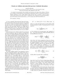
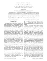
4584 PEDRO G. FERREIRA AND JOÃO MAGUEIJO56A useful discussion of the different cosmic microwavebackground CMB patterns imprinted by the unperturbedanisotropic expansion is presented in 5. The patterns can beroughly said to be constructed out of two ingredients: afocusing of the quadrupole when 1 and a spiral patternwhen x is finite. The Bianchi type-VII h is most general formof homogeneous, anisotropic universes in an 1 which areasymptotically Friedmann-Robertson-Walker. The pattern isof the formTT f 1cos˜.34In each const circle the pattern has a dependence in ofthe form cos(˜). The phase ˜ depends on , and hencethe spiralling of the simple cold and hot bump induced by thecos dependence. The functions f 1 () and ˜() are rathercomplicated functions which have to be evaluated numerically,and depend on various details of the particular Bianchimodel within the type we have chosen. It is curious to note,however, that only the power spectrum C l and the phases are sensitive to these details. All the spirals imprinted byBianchi type-VII h models have moduli of the form m l m1 f 2 l,x.Therefore their shape spectra will always beB m l 1,for 2ml,35B m l 0, for m1. 36The background patterns in Bianchi type-VII h models are alllocalized, shapeful, and connected structures. Depending onthe model they will however have different positions, powerspectra, and connectivity. Nevertheless, their shape spectra isalways the same exact shape, of form 36, without any cosmicvariance error bars. Confusion with a Gaussian is zero.Confusion with the shape of a perfect texture hot spot is zeroas well. These have a non-Gaussian spectrum of the formB m l 1, for 1ml. 37lAlthough the shape spectrum is the same up to the last B m ,the confusion between the two theories is zero. Of coursereal textures are not perfect circular spots. Cosmic variancein their irregularities will further complicate the problem.lNevertheless some sort of peak around this B m predictionshould exist in real life.VII. ANISOTROPIC GAUSSIAN FLUCTUATIONSIN BIANCHI MODELSIn the previous section we explored the fact that in Bianchimodels the CMB is not isotropic even before fluctuationsare introduced. A rather non-Gaussian spiral pattern of form34 is imprinted by the universal rotation on the CMB. Thispattern is obviously non-Gaussian and is a localized feature.It is therefore not hard to place tight constraints on anisotropyon the grounds of this prediction. A possibility remainshowever that anisotropy might manifest itself in a moresubtle way. Anisotropic expansion would certainly affect theFIG. 1. An isotropic Gaussian map as seen with a resolution ofabout 20°. The power spectrum was assumed to be scale invariant.production of Gaussian fluctuations. From what we have saidin Sec. V it is clear that anisotropic Gaussian fluctuationscould escape detection much more easily. They are delocalizednon-Gaussian features, and most non-Gaussian tests, includingour eyes, target localization. As shown in 19 delocalizedfeatures escape traditional methods of non-Gaussiandetection. These include skewness and kurtosis, the threepointcorrelation function, density of peaks above a givenheight, genus number of isotemperature lines, and the ubiquitousplotting of pixel histograms. We will reiterate thispoint here with one class of anisotropic Gaussian fluctuations.Let us consider anisotropic Gaussian fluctuations with acovariance matrix of forma l m a l m* mm ll C lm .38These theories are characterized by an angular power spectrumwhich is now a function of two indices, l and m. IsotropicGaussian theories may be regarded in this context as aparticular type of spectrum in the m dimension: they arewhite noise in m that is, the power is constant as a functionof m. Anisotropy manifests itself in the form of departuresfrom white noise in the m dimension of the power spectrum.These departures may in principle take any functional form,but for simplicity let us consider a linear dependence, that is,we merely tilt the white noise spectrum. ThenC lm C l nm,39where is defined so that C l is indeed the angular powerspectrum. We call n the m-tilt. An isotropic theory has zerom-tilt. A positive m-tilt will favor high azimuthal frequencies,a negative tilt will favor modes which disrupt strictcylindrical symmetry the least, that is low m modes. Thelarger the m-tilt the more anisotropic the fluctuations are. Forevery l a critical tilt n* exists beyond which some m modesdo not receive any power. We may consider exceeding thistilt unreasonable.In Fig. 1 we produced an isotropic Gaussian map with aresolution of 20° and a scale-invariant power spectrum. InFig. 2 we produced an anisotropic Gaussian map with thesame power spectrum, and using the same random numbers.The tilt is the critical negative tilt n*. It is curious to notehow similar the two maps are. The point is that it is thephases that determine what the maps look like and they arethe same random phases in both maps. Clearly it will be

56 CLOSET NON-GAUSSIANITY OF ANISOTROPIC ...4585FIG. 2. An anisotropic Gaussian map obtained with the samerandom numbers as in Fig. 1. However this theory is maximallytilted in m in all scales. Since the azimuthal phases are random, andthey are the same in both realizations the outcome looks the same,although this map is extremely anisotropic, or, from the point ofview of an isotropic formalism, extremely non-Gaussian.difficult to identify the anisotropy, or equivalently the non-Gaussianity, of m-tilted maps. They will look very Gaussianand isotropic even for the large tilt n*.One would have to do something extreme, such as considern, for the anisotropy of m-tilted theories to becomeobvious. The map in Fig. 3 has the same power spectrumand random number as the two previous maps but it hasn. This means that the mode m0 receives all thepower for any l. The surprise now is that the map obtained isGaussian at all, in some sense. The features shown in thismaps appear to be not only blatantly anisotropic, but alsovery non-Gaussian.It should not come as a surprise that for any theory with areasonable m-tilt classic Gaussian tests will fail to detect thenon-Gaussianity. We exemplify this with skewness 3 andkurtosis 4 . In all anisotropic Gaussian theories with nn* the average 3 and 4 are always well within the cosmicvariance error bar for a Gaussian. In no case could weFIG. 3. A theory with exact cylindrical symmetry in all realizationsis an extreme case of Gaussian anisotropic fluctuation. Thismap has still the same random numbers as before. Now it doesbecome obvious that the theory is non-Gaussian isotropic, or anisotropicin the first place.decide between isotropic and anisotropic Gaussian theorieson the grounds of their 3 and 4 . The situation is evenworse if n is not too much larger then n*/2. Then the distributionsof 3 and 4 are in practice the same for isotropicand anisotropic Gaussian fluctuations. We show this fact inFig. 4, where we plotted histograms of skewness and kurtosisfrom an isotropic Gaussian theory, and an anisotropic Gaussiantheory with the same power spectrum and m-tilt nn*/2/2. This plot shows that not only that 3 and 4 cannotbe used to distinguish between the theories, but also thethe theories are statistically the same as far as 3 and 4 areconcerned.lIn spite of the failure of classical tests, the B m should stilldetect the non-Gaussianity in m-tilted maps. They contain alllldegrees of freedom in the a m apart from the phases mwhich are Gaussian in these theories. Therefore if the initiallla m are non-Gaussian the B m have to accuse their nonlGaussianity. In Fig. 5 we plot B m spectra for an isotropicGaussian theory and for a theory with nn*/2. We choseFIG. 4. Histograms of skewness left and kurtosis right obtained from 8000 realizations for an isotropic Gaussian theory line and ananisotropic Gaussian theory with half the maximal transverse tilt n* on all scales.

4586 PEDRO G. FERREIRA AND JOÃO MAGUEIJO56FIG. 5. The B 10 m spectra with errorbars for an isotropic Gaussian theory and for an anisotropic Gaussian theory with nn*/2. The errorlbars are misleading as the distributions may not be peaked. In particular the B m distribution in the Gaussian case is simply uniform.lNevertheless it should be obvious that a peaked distribution is emerging in some B m in the bottom plot. These correspond to the emergenceof preferred shapes in these theories.multipole l10 and in analogy with C l spectra plotted ourresults in the form of an average and a 1 error bar. Thismay be misleading. For instance in the isotropic Gaussiancase the distributions are simply uniform distributions, forwhich the average 1/2 does not represent any favored valuewhere the distribution peaks. Also the distributions for anisotropicGaussian theories are very skewed and tend to bemore peaked than their error bars suggest. Hence this methodover rates confusion with a Gaussian. Even so it is clear thatdepartures from uniformity are being observed, at least insome m’s. Peaked distributions are emerging and concept oflB m spectrum is acquiring a meaning, in the same way C lspectra are meaningful.lIn Fig. 6 we plot histograms of various B m for a tiltedFIG. 6. The distributions of B 10 9 line, left, B 10 7 dash, left, B 10 5 line, right, and B 10 1 dash, right, for a tilted theory with nn*/2.lAlthough for small m the B m are still very Gaussian, for m close to l the distributions peak around 1. Recall that for an isotropic Gaussianltheory all B m should be uniformly distributed.

56 CLOSET NON-GAUSSIANITY OF ANISOTROPIC ...4587theory with nn*/2. These show much more clearlywhere the peak value is obtained and what the error barllshould be for the B m . For m close to l the B m distributionspeak at 1, falling off more steeply the closer to l the m. Itisonly for low m that the distributions become again very closeto uniform.Although we have chosen nn*/2 in the above discussionthe method described applies for lower values of transversetilt. It is important to realize that the B m contain all thellnon-Gaussian degrees of freedom in the a m for anisotropicGaussian theories, and therefore they have to detect non-Gaussianity should there be any. One must realize that thelB m are not a single statistic but a whole spectrum of statistics,and that even a faint signal in only some of the l and mwould combine into a rather powerful signal when the wholespectrum is taken into account.VIII. AN ANISOTROPIC GRISCHUK-ZEL’DOVICHEFFECTWe shall now consider an example of a flat homogeneousand isotropic universe with topological identification alongone axis. This example is simpler than most of those consideredin the literature but illustrates one of the key features ofsuch models: the breaking of statistical isotropy in the fluctuations.Let us consider a universe with a topological identificationalong the z axis. All functions defined on such aspace satisfyx,y,zx,y,zL.40By considering a flat universe we can restrict ourselves tocalculating the Sachs-Wolfe effect. The temperature anisotropyfrom the surface of last scattering will be given byTT n 1 2H 02c 2e d 2 kjin–q kjq 2 , 41where 0 ls is radius of the surface of last scatter andqkcos,ksin,2( j/L).The a lm’ s are given bya lm il2H 02c 2 d 2 kj kjj l qq 2 Y lm* qˆ. 424ill H 0a lm* a l m 4 c 4 mm kdkjP˜lmqˆpˆ l m qˆ.j l qj l qq 345It is convenient to define k and j 2 j where /L, i.e., the ration of our horizon to the topological identificationscale. If we now define y j / 2 j 2 the expressionsimplifies toill H 4 j0 1a lm* a l m 4 c 4 mm dy0l jyj l jyjP˜lmyP˜lm y. j46In the limit where the identification scale goes to infinitywe get the standard result1lim a lm* a l m dyjl→002 1 y ll mm 1 l 2 ll mm ,47i.e., a scale invariant, diagonal covariance matrix. In the caseof finite this is not the case. Consider the quadrupole. Thering spectra has two components, B 1 and B 2 with a probabilitydistribution functionFr,B 1 ,B 2 /2 1/2 3 2 3!! expr2 /2 2 2 c 0 B 2 3/21 B 2where we have definedr 4c 1 B 2 3/2 1B 1 2 c 2 1B 3/2 , 2 2 a 20 2 a 21 2 a 22 2 1/3 ,c i 22a 2i 2 .4849By exploring the dependence of c 0 , c 1 , and c 2 on we cansee how the probability distribution function of the B’schange with topology scale; to a very good approximationwe findWe now assume statistical homogeneity and isotropy of and a scale invariant power spectrumc 0 1522122 2 ,c 1 1328152 8 , kj* k j 2 kk jj q 1 qk 2 2j/L 2 43This leads to the covariance matrix for the a lm ’s:4ill H 0 ja lm* a l m 4 c 4 d 2 kl qj l qj q 3Y lm* qˆY l m qˆ.44Expressing Y lm (n)P˜lm(cos)e im and performing theazimuthal integral, one immediately finds that the covariancematrix is diagonal in m, so one hasc 2 17221102 2 .50We can see the signature for non-Gaussianity arising here.For a nonzero there are correlations between the threestatistical quantities. The probability distribution function forB 1 and B 2 defined on 0,10,1 becomes peaked at 1.We have focused on the quadrupole where the effect is easyto see. The method is systematic however, and one can constructthe probability distribution function of the high orderring spectra in the same way.To exemplify the strength of the technique we shall contrastit with two standard measures of non-Gaussianity, the

4588 PEDRO G. FERREIRA AND JOÃO MAGUEIJO56FIG. 7. A comparison of the probability distribution function of skewness left panel and kurtosis right panel for an anisotropicensemble solid line with 1 and am isotropic, Guassian ensemble dashed line with the same power spectrum.skewness, 3 , and kurtosis, 4 . Unlike with our method,where one can calculate the probability distribution functionanalytically, for these more conventional methods one has toresort to Monte Carlo simulations. The procedure for generatingtopologically anisotropic skies is a slight modificationof the one proposed in 21 for generating isotropic skies. Inthe latter, one generates an uncorrelated set of a lm the covariancematrix is diagonal. Given a nondiagonal covariancematrix C ii a lm* a l m where il(l1)m1 il(l1)m1, one can Cholesky decompose it, CLL T . One can then generate a set of uncorrelated randomnumbers, r from a Gaussian distribution with 0 mean andunit variance. The vector sLr will satisfy s i s i C ii andtherefore is a set of a lm with the correct covariance matrix.In Fig. 7 we show the results for two ensembles of 1000realizations. In one ensemble A we generate skies with an2, each realization having a random orientation. The rival,Gaussian ensemble I has as many Gaussian realizationsof skies with the same power spectrum as ensemble A.Clearly we are well within the region where the probabilitydistribution function for the shape spectra deviates fromunity c 0 5/2, c 2 3/5, and c 1 7/10. In Fig. 7, we plot thehistograms for 3 and 4 . Although 3 for ensemble A hasa marginally larger variance than ensemble B it is clear thatin practice it is difficult to disentangle the two. The probabilitydistribution functions for 4 are, in practice, indistinguishable.This to be compared to Fig. 8 where we plot theratio of the joint probability distribution function for a fixedr of the completely anisotropic case relative to the completelyisotropic case. There is a clear departure from uniformity.This a curious application of the idea put forward in 22,an anisotropic Grischuk-Zel’Dovich effect. By looking at theshape of the low l multipole moments we can constrain thedegree of statistical anisotropy outside the current horizon.Note that, already for 1 there are deformations in thecovariance matrix which may be statistically significant withcurrent data. This will be pursued in a future publication23.IX. CONCLUSIONSIn this paper we have presented a new technique for quantifyingnon-Gaussianity on large scales. It is the extension ofthe non-Gaussian spectra developed in 19 to the surface ofthe two sphere. As we have shown in Sec. II the constructionis slightly different to take into account the particularities ofFIG. 8. A comparison of the joint probability distribution functionof B 1 and B 2 for the isotropic and completely anisotropic case.For r 2 /(2 2 2 )1 we plot ratio of the anisotropic likelihood functionto the isotropic likelihood function. Recall that for an isotropictheory the B’s are uniformly distributed.

56 CLOSET NON-GAUSSIANITY OF ANISOTROPIC ...4589the spherical harmonic basis. However the qualititative interpretationof the different levels of non-Gaussianity followsthrough, exactly as in 19. One can identify the informationcontained in the ring, interring and phase spectra with shape,connectivity and localization.An interesting and untapped application is to universeswith statistically anisotropic fluctuations. Developing theidea put forward in 10 we explain how statistical anisotropyand non-Gaussianity are intimately related. From thisone can infer some novel properties of the covariance matrixof fluctuations in statistically anisotropic spacetimes. In particular,features which appear in non-Gaussian theories ofstructure formation, like textures 11,12 will appearhere: a surplus of cosmic variance and cosmic covarianceof the power spectra.There are a number of situations where these results areapplicable. One is in the case of anisotropic universes, i.e.,universes which are not Friedmann-Robertson-Walker universes.There are a number of known examples 1,2. Withoutactually doing perturbation theory on them we argue fora natural prescription for adding fluctuations in the CMB tosuch models. It consists of finding the reduced symmetrygroup of the temperature patterns and constructing anisotropicGaussian random fields with such properties in whichthe covariance matrix satisfies those symmetries, and notmore. In fact it can be shown that these symmetries can bededuced from the geodesic structure of the space time 24.This can be a first step in extending the prescription used in6 for constraining general anisotropic models with the CosmicBackground Explorer COBE four year data. A briefanalysis is made of the relevant Bianchi models for whichwe present the non-Gaussian spectra.Another, different application is the case of homogeneousisotropic models where an anisotropic topological identificationhas been imposed. As an example we identify one directionin space. One finds that statistical isotropy is broken.This can be easily from the following: if we look along theaxis of identification, and the identification scale is smallerthan our horizon, one will find strong correlations betweenpatches of the microwave sky which are reflected about theuncompactified plane 7. By looking at the structure of thecovariance matrix one can see that this anisotropy will manifestitself by inducing not only non-Gaussian ring spectra butalso inter-ring spectra. This non-Gaussian manifestation maypersist if we consider the identification scale to be large thanour horizon. We name this effect the anisotropic Grischuk-Zel’Dovich effect.Although we now have a high quality measurement ofanisotropies on large angular scales we are confronted withthe hardships of the real world. Galactic contamination leadsone to consider an anisotropic rendition of the sky and considerablycomplicates the analysis of the COBE four yeardata. It is well known that one of the consequences is that thequadrupole measurement should be viewed with scepticism.Unfortunately it is the quadrupole which could supply uswith a probe of primordial CMB on the largest angularscales. There may be ways around these shortcomings. Onecan try and reformulate our non-Gaussian spectra on thelargest angular scales using the techniques put forward in25. This would involve a proper likelihood analysis and tomake the problem tractable one would need to find an adequateparametrization of the non-Gaussian spectra. The factthat we have devised a consistent method for characterizingnon-Gaussianity on all scales may allow us to use the cumulativeinformation of all l2 to infer the behavior on largescales; all modes will be affected to some extent by largescale anisotropy. Finally it would be interesting to analyze inmore detail the observability of the anisotropic Grischuk-Zel’Dovich effect, taking into consideration issues of cosmicvariance.ACKNOWLEDGMENTSWe would like to thank T Kibble for pointing out andcorrecting a serious mistake at the heart of this paper. J.M.thanks MRAO-Cambridge for use of computer facilitieswhile this paper was being prepared. P.G.F. gratefully acknowledgesinsightful comments from A. Anderson, C. Balland,J. Levin, A. Jaffe, and J. Silk. We thank A. Jaffe forsuggesting the numerical technique used in Sec. VIII. P.G.F.was supported by the Center for Particle Astrophysics, aNSF Science and Technology Center at UC Berkeley, underCooperative Agreement No. AST 9120005. J.M. was supportedby the Royal Society.APPENDIX A: GAUSSIAN FLUCTUATIONSWITH A SYMMETRYIn this appendix we detail the group theory argumentsketched in Sec. III. This argument is not necessary in theSO2 case targeted in this paper, where the covariance matrixmay be easily derived directly. However, it opens doorsto more general anisotropic symmetry groups. It also showshow the general form of the covariance matrix depends noton the symmetry group, but only on its irreducible representationsirreps.Fluctuations Gaussian or not in any universe must besubject to the symmetries of the underlying cosmologicalmodel. However, due to the random nature of the fluctuations,they must satisfy these symmetries only statistically.By this we mean that the statistical ensemble of fluctuations,and not each realization, should be subject to the symmetries.If a symmetry transformation is applied to each member ofthe ensemble, then each member may change, but the ensembleshould remain the same. For instance, for the SO3symmetry group only realizations containing only a monopolel0 are left unchanged by rotations. Nevertheless muchmore general fluctuations respect statistical isotropy. Similarly,only the m0 modes are cylindrically symmetric, butmore general fluctuations are SO2 statistically invariant. 5Gaussian fluctuations are fully specified by their covariancematrixlC 1 l 2 l 1 l am1m1a 2*m 2 m2,A15 Some texture models exhibit approximate SO2 symmetry atlow l in each realization. Then an axes system exists in which them0 mode has much more power than any other. This is of coursea very non-Gaussian effect which cannot be simply reproduced byanisotropic Gaussian fluctuations.

4590 PEDRO G. FERREIRA AND JOÃO MAGUEIJO56which may be seen as a bilinear form on the a l m space.Hence the statistical symmetries of a Gaussian theory areequivalent to the requirement that the covariance matrix isleft unchanged by any symmetry transformation. Let G bethe symmetry group of the underlying cosmological modelas projected on the sky. Let us first suppose that G breaks thea l m into a set on nonequivalent irreps. Then, let us find anew basis a LM adapted to G, where L now labels the irrep thebasis element belongs to, and M the actual element. Then GLis represented by a set of matrices G MMacting on a LM asã L M Ga L LM G MMThe covariance matrix for the a M L ,La M . A2LC 1 L 2 LMa 1 L1 M 2 Ma 2*1 M,A32must remain unchanged by the transformation A2, so thatLC˜ 1 L 2 Lã 1 LM 1 M 2 Mã 2*L 1 L1 MG2 M 1 M G 2* L1 M 2 M C 1 L 2 L2 MC 1 L 21 M 2 M,1 M 2A4which for unitary representations amounts to the commutationrelationG L 1C L 1 L 2C L 1 L 2G L 2.A5Let us now recall Schur’s Lemmas 20.Schur’s Lemma 1. Let and be two irreps of a groupG with dimensions d and d, and let there be a dd matrixA such thatgAAgA6for all group elements g. Then either A0 or dd anddet A0.It follows that if A0 then and are equivalent.Schur’s Lemma 2. If is a d-dimensional irrep of a groupG and B is a dd matrix such thatgBBgA7for all group elements g, then B1.Combining the two Lemmas we can then find that thecovariance matrix must take the formLC 1 L 2 LMã 1 L1 M 2 Mã 2*1 M L 1 L 2 M 21 M 2C L1 .A8An interesting result is that if G breaks the a m l space intonon-equivalent irreps spanned by a M L , then these must beindependent random variables with a variance which canonly depend on the irrep they belong to. This argument appliesfor instance if the symmetry group is SO3, in whichcase Ll and Mm.The argument just present breaks down however, if someof the irreps defined by G are equivalent. Let the a m l spacenow be spanned by an adapted basis a M LD , where L labelseach class of equivalent representations, D labels the actualirrep within this class, and M labels the elements within eachIrrep. Then, from the second Schur’s Lemma we know thatwithin the same irrep we still havea LD M a LD 1 M2* M1 M 2C LD ,A9but for different but equivalent irreps (D 1 D 2 ) we nowhaveLDa 1 LDMa 2* LD1M2C 1 D 2M1 M A102with det C0, whereas for nonequivalent irreps (L 1 L 2 )we still haveLa 1 D 1 LMa 2 D 2*1 M0.A112Therefore, although the a LD M are independent within each irrepand among different non-equivalent irreps, correlationsmay exist between different but equivalent irreps. Of courseone may always rotate the a LD M within each class of equivalentirreps so as to diagonalize the covariance matrix. Howeversuch a rotation is model dependent, and cannot be determinedfrom the symmetries. This situation happens forinstance in the case of SO2, with Lm and Dl no Mindex, since the irreps are one dimensional. Each m providesa class of equivalent representations, with the same mbut different l. Then the covariance matrix takes the generalformla 1 lm1a 2* lm2 m1 m 2C 1 l 2m1A12and as we see although correlations among different m arenot allowed, now we may have correlations between differentl, for the same m. We could rotate the a m in l for eachlfixed m so as to diagonalize the covariance matrix, but suchprocedure naturally would depend on the covariance matrixone starts from, and would therefore be model dependent.1 G. Ellis and M. MacCallum, Commun. Math. Phys. 12, 1081969.2 A. Krasinski, Inhomogeneous Cosmological Models CambridgeUniversity Press, Cambridge, England, 1996.3 J. Barrow private communication.4 C. B. Collins and S. W. Hawking, Mon. Not. R. Astron. Soc.162, 307 1973.5 J. D. Barrow, R. Juszkiewicz, and D. Sonoda, Mon. Not. R.Astron. Soc. 213, 917 1985.6 E. Bunn, P. Ferreira, and J. Silk, Phys. Rev. Lett. 77, 28831996.7 A. De Oliveira Costa, G. Smoot, and A. Starobinsky, Astrophys.J. 468, 457 1996.8 J. J. Levin, J. D. Barrow, E. F. Bunn, and J. Silk, Phys. Rev.Lett. 79, 974 1997.9 J. Kogut et al., astro-ph/9601062.10 J. Magueijo, Phys. Lett. B 342, 321995; 352, 499 E 1995.11 J. Magueijo, Phys. Rev. D 52, 689 1995.

56 CLOSET NON-GAUSSIANITY OF ANISOTROPIC ...459112 J. Magueijo, Phys. Rev. D 52, 4361 1995.13 D. Coulson, P. Ferreira, P. Graham, and N. Turok, NatureLondon 368, 271994.14 U. Pen, D. Spergel, and N. Turok, Phys. Rev. D 49, 6921994.15 N. Turok, Astrophys. J. 473, L51996.16 B. Allen et al., Phys. Rev. Lett. 77, 3061 1996.17 A simple example is supplied in 12: an inflationary theorywhich predicts a random tilt.18 C. Cheung and J. Magueijo, ‘‘Unpredictable explosions’’ inpreparation.19 P. G. Ferreira and J. Magueijo, Phys. Rev. D 55, 3358 1997.20 J. F. Cornwell, Group Theory in Physics Academic Press,London, 1990.21 J. Bond and G. Efstathiou, Mon. Not. R. Astron. Soc. 226, 6651987.22 L. P. Grishchuk and Ya. B. Zel’Dovich, Astron. Zh. 55, 2091978.23 P. G. Ferreira and J. Magueijo in preparation.24 J. D. Barrow and J. J. Levin, astro-ph/9704041.25 K. M. Gorski et al., astro-ph/9601063.