LISALISA - iucaa

LISA
Laser Interferometer Space Antenna: A Cornerstone
Mission for the Observation of Gravitational Waves
System and Technology Study Report

LISA
Laser Interferometer Space Antenna
A Cornerstone Mission for the observation of
gravitational waves
System and Technology Study Report
ESA-SCI(2000)11 July 2000

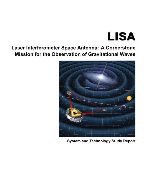
Front cover figure :
Artist’s concept of the LISA configuration, bathing in the gravitational waves emitted from a
distant cosmic event.
Three spacecraft, each with a Y-shaped payload, form an equilateral triangle with sides of
5 million km in length. The two branches of the Y at one corner, together with one branch
each from the spacecraft at the other two corners, form one of up to three Michelson-type
interferometers, operated with infrared laser beams. The interferometers are designed to measure
relative path changes δl/l due to gravitational waves, so-called strains in space, down to 10 −23 ,
for observation times of the order of 1 year.
The diameters of the spacecraft are about 2.5 m, the distances between them 5×10 9 m.
Rear cover figure :
Schematic diagram of LISA configuration, with three spacecraft in an equilateral triangle. The
plane of this triangle is tilted by 60 ◦ out of the ecliptic. The center of this triangle moves around
the Sun in an Earth-like orbit, about 20 ◦ behind the Earth, with the plane of the LISA formation
revolving once per year on a cone of 30 ◦ half-angle.
The drawing is not to scale, the triangular formation of the LISA interferometer, with sides of
5 million km, is blown up by a factor of 5.
13-9-2000 11:47 ii Corrected version 1.04

LISA Mission Summary
Objectives:
Payload:
Orbit:
Launcher:
Detection of low-frequency (10 −4 to 10 −1 Hz) gravitational radiation with
a strain sensitivity of 4×10 −21 / √ Hz at 1 mHz.
Abundant sources are galactic binaries (neutron stars, white dwarfs, etc.);
extra-galactic targets are supermassive black hole binaries (SMBH-SMBH
and BH-SMBH), SMBH formation, and cosmic background gravitational
waves.
Laser interferometry with six electrostatically controlled drag-free reference
mirrors housed in three spacecraft; arm lengths 5×10 6 km.
Each spacecraft has two lasers (plus two spares) which operate in a phaselocked
transponder scheme.
Diode-pumped Nd:YAG lasers: wavelength 1.064 µm, output power 1 W,
Fabry-Perot reference cavity for frequency-stability of 30 Hz/ √ Hz.
Quadrant photodiode detectors with interferometer fringe resolution,
corresponding to 4×10 −5 λ/ √ Hz.
30 cm diameter f/1 Cassegrain telescope (transmit/receive), λ/10 outgoing
wavefront quality.
Drag-free proof mass (mirror): 40 mm cube, Au-Pt alloy of extremely low
magnetic susceptibility (< 10 −6 ); Ti-housing at vacuum < 10 −6 Pa;
six-degree-of-freedom capacitive sensing.
Each spacecraft orbits the Sun at 1 AU. The inclinations are such that
their relative orbits define a circle with radius 3×10 6 km and a period of
1 year. The plane of the circle is inclined 60 ◦ with respect to the ecliptic.
On this circle, the spacecraft are distributed at three vertices, defining
an equilateral triangle with a side length of 5 × 10 6 km (interferometer
baseline).
This constellation is located at 1 AU from the Sun, 20 ◦ behind the Earth.
Delta II 7925 H, 10 ft fairing, housing a stack of three composites consisting
of one science and one propulsion module each.
Each spacecraft has its own jettisonable propulsion module to provide a
∆V of 1300 m/s using solar-electric propulsion.
Spacecraft:
mass:
propulsion module:
propellant:
total launch mass:
power:
power:
3-axis stabilized drag-free spacecraft (three)
274 kg, each spacecraft in orbit
142 kg, one module per spacecraft
22 kg, for each propulsion module
1380 kg
940 W, each composite during cruise
315 W, each spacecraft in orbit
Drag-free performance: 3×10 −15 m/s 2 (rms) in the band 10 −4 to 3×10 −3 Hz, achieved with 6×4
Cs or In FEEP thrusters
Pointing performance: few nrad/ √ Hz in the band 10 −4 Hz to 1 Hz
Payload, mass: 70 kg, each spacecraft
power:
72 W, each spacecraft
Science data rate: 672 bps, all 3 spacecraft
Telemetry:
7 kbps, for about 9 hours inside two days
Ground stations: Deep Space Network
Mission Lifetime:
2 years (nominal); 10 years (extended)
Corrected version 1.04 iii 13-9-2000 11:47

13-9-2000 11:47 iv Corrected version 1.04

Foreword
The first mission concept studies for a space-borne gravitational wave observatory began 1981
at the Joint Institute for Laboratory Astrophysics (JILA) in Boulder, Colorado. In the following
years this concept was worked out in more detail by P.L. Bender and J.Faller and in 1985 the
first full description of a mission comprising three drag-free spacecraft in a heliocentric orbit was
proposed, then named Laser Antenna for Gravitational-radiation Observation in Space (LAGOS).
LAGOS already had many elements of the present-day Laser Interferometer Space Antenna
(LISA) mission.
In May 1993, the center of activity shifted from the US to Europe when LISA was proposed
to ESA in response to the Call for Mission Proposals for the third Medium-Size Project (M3)
within the framework of ESA’s long-term space science programme “Horizon 2000”. The proposal
was submitted by a team of US and European scientists coordinated by K.Danzmann, Max-
Planck-Institut für Quantenoptik and Universität Hannover. It envisaged LISA as an ESA/NASA
collaborative project and described a mission comprising four spacecraft in a heliocentric orbit
forming an interferometer with a baseline of 5×10 6 km.
The SAGITTARIUS proposal, with very similar scientific objectives and techniques, was proposed
to ESA at the same time by another international team of scientists coordinated by
R.W. Hellings, JPL. The SAGITTARIUS proposal suggested placing six spacecraft in a geocentric
orbit forming an interferometer with a baseline of 10 6 km.
Because of the large degree of commonality between the two proposals ESA decided to merge
them when accepting them for a study at assessment level in the M3 cycle. It was one of the main
objectives of the Assessment Study to make an objective trade-off between the heliocentric and
the geocentric option. The Study Team decided to adopt the heliocentric option as the baseline
because it has the advantage that it provides for reasonably constant arm lengths and a stable
environment that gives low noise forces on the proof masses, and because neither option offered
a clear cost advantage.
Because the cost for an ESA-alone LISA (there was no expression of interest by NASA in a
collaboration at that time) exceeded the M 3 cost limit, it became clear quite early in the
Assessment Study that LISA would not be selected for a study at Phase A level in the M 3 cycle.
In December 1993, LISA was therefore proposed as a cornerstone project for “Horizon 2000 Plus”,
involving six spacecraft in a heliocentric orbit. Both the Fundamental Physics Topical Team
and the Survey Committee realised the enormous discovery potential and timeliness of the LISA
Project and recommended it as a cornerstone of “Horizon 2000 Plus”.
Being a cornerstone in ESA’s space science programme implies that, in principle, the mission is
approved and that funding for industrial studies and technology development is provided right
away. The launch year, however, is dictated by the availability of funding.
In 1996 and early 1997, the LISA team made several proposals how to drastically reduce the
cost for LISA without compromising the science in any way, most importantly to reduce the
number of spacecraft from six to three, where each of the new spacecraft would replace a pair
of spacecraft at the vertices of the triangular configuration, with essentially two instruments in
each spacecraft. With these and a few other measures the total launch mass could be reduced
from 6.8 t to 1.4 t.
Perhaps most importantly, it was proposed by the LISA team and by ESA’s Fundamental Physics
Advisory Group (FPAG) in February 1997 to carry out LISA in collaboration with NASA. A
launch in the time frame 2010 would be ideal from the point of view of technological readiness of
the payload and the availability of second-generation detectors in ground-based interferometers
Corrected version 1.04 v 13-9-2000 11:47

Foreword
making the detection of gravitational waves in the high-frequency band very likely.
In January 1997, a candidate configuration of the three-spacecraft mission was developed by
the LISA science team, with the goal of being able to launch the three spacecraft on a Delta-
II. The three-spacecraft LISA mission was studied by JPL’s Team-X in January, 1997 . The
purpose of the study was to assist the science team, represented by P.L. Bender and R.T. Stebbins
(JILA/University of Colorado), and W.M. Folkner (JPL), in defining the necessary spacecraft
subsystems and in designing a propulsion module capable of delivering the LISA spacecraft into
the desired orbit. The result of the Team-X study was that it appeared feasible to fly the threespacecraft
LISA mission on a single Delta-II 7925 H launch vehicle by utilizing a propulsion
module based on a solar-electric propulsion, and with spacecraft subsystems expected to be
available by a 2001 technology cut-off date.
In June 1997, a LISA Pre-Project Office was established at JPL with W.M. Folkner as the Pre-
Project Manager and in December 1997, an ad-hoc LISA Mission Definition Advisory Team was
formed by NASA. Representatives from ESA’s LISA Study Team are invited to participate in
the activities of the LISA Mission Definition Team.
The revised version of LISA (three spacecraft in a heliocentric orbit, ion drive, Delta-II launch
vehicle; NASA/ESA collaborative) has been endorsed by the LISA Science Team and served as
the basis for a detailed payload definition study by the LISA team. After a payload review in
April 1998, ESA’s Fundamental Physics Advisory Group (FPAG) concluded that the payload
had reached a sufficient level of maturity and recommended to enter into the industrial study
phase.
This industrial System and Technology Study was performed by a consortium consisting of
Dornier Satellitensysteme (Germany) as the prime and Alenia (Italy) and Matra (France) as
subcontractors with intensive involvement of the LISA Science Team throughout the study. The
System and Technology Study was begun in June 1999 and the final report delivered to ESA in
June 2000. It is based on a collaborative ESA/NASA mission with equal shares and a launch
in 2010. This is the baseline scenario that is now also part of NASA’s Strategic Plan.
The industrial study was performed by the following team members:
Industrial Team Manager :
A. Hammesfahr, Dornier Satellitensysteme
Industrial Team :
H. Faulks, K. Gebauer, K. Honnen, U. Johann, G. Kahl, M. Kersten, L. Morgenroth,
M. Riede, and H.-R. Schulte from Dornier Satellitensysteme,
M. Bisi and S. Cesare from Alenia Aerospazio,
O. Pierre, X. Sembely, and L. Vaillon from Matra Marconi Space,
D. Hayoun, S. Heys, and B.J. Kent from Rutherford Appleton Laboratory,
F. Rüdenauer from Austrian Research Center Seibersdorf,
S. Marcuccio and D. Nicolini from Centrospazio,
L. Maltecca from Laben S.p.A. and
I. Butler from University of Birmingham.
ESOC Support:
Jose Rodriguez-Canabal
13-9-2000 11:47 vi Corrected version 1.04

Foreword
The ESA personnel from the Directorate of the Scientific Programme assiociated with the study
were :
R. Reinhard (acting Study Scientist and ESA-HQ Fundamental Physics Missions
Coordinator)
T. Edwards(Study Manager under contract to ESA, Rutherford Appleton Laboratory)
LISA Study Team :
P. Bender, Joint Institute for Laboratory Astrophysics, Boulder, Colorado, USA
A. Brillet, Observatoire de la Côte d’Azur, Nice, France
A.M. Cruise, University of Birmingham, UK
C. Cutler, Albert-Einstein Institut, Potsdam, Germany
K. Danzmann, Max-Planck-Institut für Quantenoptik and Universität Hannover, Germany
F. Fidecaro, INFN, Pisa, Italy
W.M. Folkner, Jet Propulsion Laboratory, Pasadena, California, USA
J. Hough, University of Glasgow, UK
P. McNamara, University of Glasgow, UK
M. Peterseim, Max-Planck-Institut für Quantenoptik, Hannover, and LZH, Germany
D. Robertson, University of Glasgow, UK
M. Rodrigues, ONERA, France
A. Rüdiger, Max-Planck-Institut für Quantenoptik, Garching, Germany
M. Sandford, Rutherford Appleton Laboratory, Chilton, UK
G. Schäfer, Universität Jena, Germany
R. Schilling, Max-Planck-Institut für Quantenoptik, Garching, Germany
B. Schutz, Albert-Einstein Institut, Potsdam, Germany
C. Speake, University of Birmingham, UK
R.T. Stebbins, Joint Institute for Laboratory Astrophysics, Boulder, Colorado, USA
T. Sumner, Imperial College, London, UK
P. Touboul, ONERA, France
J.-Y. Vinet, Observatoire de la Côte d’Azur, Nice, France
S. Vitale, Università di Trento, Italy
H. Ward, University of Glasgow, UK
W. Winkler, Max-Planck-Institut für Quantenoptik, Garching, Germany
For further information please contact Karsten Danzmann
Corrected version 1.04 vii 13-9-2000 11:47

13-9-2000 11:47 viii Corrected version 1.04

Contents
Mission Summary Table
Foreword
iii
v
Executive Summary 1
The nature of gravitational waves . . . . . . . . . . . . . . . . . . . . . . . . . . . . . 1
Sources of gravitational waves . . . . . . . . . . . . . . . . . . . . . . . . . . . . . . . 2
Complementarity with ground-based observations . . . . . . . . . . . . . . . . . . . . 3
The LISA mission . . . . . . . . . . . . . . . . . . . . . . . . . . . . . . . . . . . . . . 4
1 Scientific Objectives 7
1.1 Theory of gravitational radiation . . . . . . . . . . . . . . . . . . . . . . . . . . 7
1.1.1 General relativity . . . . . . . . . . . . . . . . . . . . . . . . . . . . . . . 7
1.1.2 The nature of gravitational waves in general relativity . . . . . . . . . . 12
1.1.3 Generation of gravitational waves . . . . . . . . . . . . . . . . . . . . . . 14
1.1.4 Other theories of gravity . . . . . . . . . . . . . . . . . . . . . . . . . . . 16
1.2 Low-frequency sources of gravitational radiation . . . . . . . . . . . . . . . . . 18
1.2.1 Galactic binary systems . . . . . . . . . . . . . . . . . . . . . . . . . . . 21
1.2.2 Massive black holes in distant galaxies . . . . . . . . . . . . . . . . . . . 25
1.2.3 Primordial gravitational waves . . . . . . . . . . . . . . . . . . . . . . . 31
2 Different Ways of Detecting Gravitational Waves 35
2.1 Detection on the ground and in space . . . . . . . . . . . . . . . . . . . . . . . 35
2.2 Ground-based detectors . . . . . . . . . . . . . . . . . . . . . . . . . . . . . . . 36
2.2.1 Resonant-mass detectors . . . . . . . . . . . . . . . . . . . . . . . . . . . 36
2.2.2 Laser Interferometers . . . . . . . . . . . . . . . . . . . . . . . . . . . . 37
2.3 Pulsar timing . . . . . . . . . . . . . . . . . . . . . . . . . . . . . . . . . . . . . 39
2.4 Spacecraft tracking . . . . . . . . . . . . . . . . . . . . . . . . . . . . . . . . . . 40
2.5 Space interferometer . . . . . . . . . . . . . . . . . . . . . . . . . . . . . . . . . 40
2.6 Early concepts for a laser interferometer in space . . . . . . . . . . . . . . . . . 41
2.7 Heliocentric versus geocentric options . . . . . . . . . . . . . . . . . . . . . . . 43
3 The LISA Concept – An Overview 45
3.1 The LISA flight configuration . . . . . . . . . . . . . . . . . . . . . . . . . . . . 45
3.2 The LISA orbits . . . . . . . . . . . . . . . . . . . . . . . . . . . . . . . . . . . 45
3.3 The three LISA spacecraft . . . . . . . . . . . . . . . . . . . . . . . . . . . . . . 46
3.4 The payload . . . . . . . . . . . . . . . . . . . . . . . . . . . . . . . . . . . . . . 48
Corrected version 1.04 ix 13-9-2000 11:47

Contents
3.4.1 The proof mass . . . . . . . . . . . . . . . . . . . . . . . . . . . . . . . . 49
3.4.2 The inertial sensor . . . . . . . . . . . . . . . . . . . . . . . . . . . . . . 49
3.4.3 The optical bench . . . . . . . . . . . . . . . . . . . . . . . . . . . . . . 49
3.4.4 The telescope . . . . . . . . . . . . . . . . . . . . . . . . . . . . . . . . . 50
3.4.5 The support structure . . . . . . . . . . . . . . . . . . . . . . . . . . . . 50
3.4.6 The thermal shield . . . . . . . . . . . . . . . . . . . . . . . . . . . . . . 50
3.4.7 The star trackers . . . . . . . . . . . . . . . . . . . . . . . . . . . . . . . 50
3.5 Lasers . . . . . . . . . . . . . . . . . . . . . . . . . . . . . . . . . . . . . . . . . 51
3.6 Data extraction . . . . . . . . . . . . . . . . . . . . . . . . . . . . . . . . . . . . 51
3.7 Drag-free and attitude control . . . . . . . . . . . . . . . . . . . . . . . . . . . . 52
3.8 Ultrastable structures . . . . . . . . . . . . . . . . . . . . . . . . . . . . . . . . 52
3.9 System options and trade-off . . . . . . . . . . . . . . . . . . . . . . . . . . . . 53
3.10 Summary tables . . . . . . . . . . . . . . . . . . . . . . . . . . . . . . . . . . . 53
4 Measurement Sensitivity 57
4.1 Interferometer response . . . . . . . . . . . . . . . . . . . . . . . . . . . . . . . 57
4.2 Noises and error sources . . . . . . . . . . . . . . . . . . . . . . . . . . . . . . . 59
4.2.1 The noise effects . . . . . . . . . . . . . . . . . . . . . . . . . . . . . . . 59
4.2.2 The noise types . . . . . . . . . . . . . . . . . . . . . . . . . . . . . . . . 59
4.2.3 Shot noise . . . . . . . . . . . . . . . . . . . . . . . . . . . . . . . . . . . 60
4.2.4 Optical-path noise budget . . . . . . . . . . . . . . . . . . . . . . . . . . 60
4.2.5 Acceleration noise budget . . . . . . . . . . . . . . . . . . . . . . . . . . 62
5 The Interferometer 65
5.1 Introduction . . . . . . . . . . . . . . . . . . . . . . . . . . . . . . . . . . . . . . 65
5.2 Phase locking and heterodyne detection . . . . . . . . . . . . . . . . . . . . . . 65
5.3 Interferometric layout . . . . . . . . . . . . . . . . . . . . . . . . . . . . . . . . 66
5.3.1 The optical bench of PPA2 . . . . . . . . . . . . . . . . . . . . . . . . . 67
5.3.2 Optical bench, revisited . . . . . . . . . . . . . . . . . . . . . . . . . . . 68
5.3.3 Telescope assembly . . . . . . . . . . . . . . . . . . . . . . . . . . . . . . 72
5.4 System requirements . . . . . . . . . . . . . . . . . . . . . . . . . . . . . . . . . 72
5.4.1 Laser power and shot noise . . . . . . . . . . . . . . . . . . . . . . . . . 72
5.4.2 Beam divergence . . . . . . . . . . . . . . . . . . . . . . . . . . . . . . . 72
5.4.3 Efficiency of the optical chain . . . . . . . . . . . . . . . . . . . . . . . . 72
5.4.4 Shot noise limit . . . . . . . . . . . . . . . . . . . . . . . . . . . . . . . . 73
5.5 Laser system . . . . . . . . . . . . . . . . . . . . . . . . . . . . . . . . . . . . . 73
5.5.1 Introduction . . . . . . . . . . . . . . . . . . . . . . . . . . . . . . . . . 73
5.5.2 Laser system components . . . . . . . . . . . . . . . . . . . . . . . . . . 75
5.6 Laser performance . . . . . . . . . . . . . . . . . . . . . . . . . . . . . . . . . . 76
5.6.1 Laser frequency noise . . . . . . . . . . . . . . . . . . . . . . . . . . . . 76
5.6.2 Laser power noise . . . . . . . . . . . . . . . . . . . . . . . . . . . . . . 77
13-9-2000 11:47 x Corrected version 1.04

Contents
5.6.3 On-board frequency reference . . . . . . . . . . . . . . . . . . . . . . . . 77
5.7 Beam pointing . . . . . . . . . . . . . . . . . . . . . . . . . . . . . . . . . . . . 78
5.7.1 Pointing stability . . . . . . . . . . . . . . . . . . . . . . . . . . . . . . . 78
5.7.2 Pointing acquisition . . . . . . . . . . . . . . . . . . . . . . . . . . . . . 79
5.7.3 Final focusing and pointing calibration . . . . . . . . . . . . . . . . . . . 79
5.7.4 Point-ahead angle . . . . . . . . . . . . . . . . . . . . . . . . . . . . . . 79
5.8 Thermal stability . . . . . . . . . . . . . . . . . . . . . . . . . . . . . . . . . . . 82
6 Inertial Sensor and Drag-Free Control 85
6.1 The inertial sensor . . . . . . . . . . . . . . . . . . . . . . . . . . . . . . . . . . 85
6.1.1 Overview . . . . . . . . . . . . . . . . . . . . . . . . . . . . . . . . . . . 85
6.1.2 CAESAR sensor head . . . . . . . . . . . . . . . . . . . . . . . . . . . . . 86
6.1.3 Electronics configuration . . . . . . . . . . . . . . . . . . . . . . . . . . . 87
6.1.4 Evaluation of performances . . . . . . . . . . . . . . . . . . . . . . . . . 90
6.1.5 Sensor operation modes . . . . . . . . . . . . . . . . . . . . . . . . . . . 91
6.1.6 Proof-mass charge control . . . . . . . . . . . . . . . . . . . . . . . . . . 91
6.2 Drag-free/attitude control system . . . . . . . . . . . . . . . . . . . . . . . . . . 92
6.2.1 Description . . . . . . . . . . . . . . . . . . . . . . . . . . . . . . . . . . 92
6.2.2 DFACS controller modes . . . . . . . . . . . . . . . . . . . . . . . . . . . 93
6.2.3 Autonomous star trackers . . . . . . . . . . . . . . . . . . . . . . . . . . 94
6.3 Accelerations directly affecting the proof-mass . . . . . . . . . . . . . . . . . . . 95
7 Signal Extraction and Data Analysis 97
7.1 Signal extraction . . . . . . . . . . . . . . . . . . . . . . . . . . . . . . . . . . . 97
7.1.1 Phase measurement . . . . . . . . . . . . . . . . . . . . . . . . . . . . . 97
7.2 Frequency-domain cancellation of laser noise . . . . . . . . . . . . . . . . . . . . 97
7.2.1 Laser noise . . . . . . . . . . . . . . . . . . . . . . . . . . . . . . . . . . 97
7.2.2 Clock noise . . . . . . . . . . . . . . . . . . . . . . . . . . . . . . . . . . 99
7.2.3 Other approaches . . . . . . . . . . . . . . . . . . . . . . . . . . . . . . . 100
7.3 Time-domain cancellation of laser phase noise . . . . . . . . . . . . . . . . . . . 100
7.4 Alternative laser-phase and optical-bench noise-canceling methods . . . . . . . 101
7.4.1 Notation and geometry . . . . . . . . . . . . . . . . . . . . . . . . . . . 102
7.4.2 Gravitational wave signal transfer function to single laser link . . . . . . 104
7.4.3 Noise transfer function to single laser link . . . . . . . . . . . . . . . . . 104
7.4.4 Combinations that eliminate laser noises and optical bench motions . . 104
7.4.5 Gravitational wave sensitivities . . . . . . . . . . . . . . . . . . . . . . . 109
7.5 Data analysis . . . . . . . . . . . . . . . . . . . . . . . . . . . . . . . . . . . . . 112
7.5.1 Data reduction and filtering . . . . . . . . . . . . . . . . . . . . . . . . . 113
7.5.2 Angular resolution . . . . . . . . . . . . . . . . . . . . . . . . . . . . . . 115
7.5.3 Polarization resolution and amplitude extraction . . . . . . . . . . . . . 121
7.5.4 Results for MBH coalescence . . . . . . . . . . . . . . . . . . . . . . . . 123
Corrected version 1.04 xi 13-9-2000 11:47

Contents
7.5.5 Estimation of background signals . . . . . . . . . . . . . . . . . . . . . . 124
8 Payload Design 127
8.1 Payload structure design concept . . . . . . . . . . . . . . . . . . . . . . . . . . 127
8.2 Payload structural components . . . . . . . . . . . . . . . . . . . . . . . . . . . 128
8.2.1 Optical assembly . . . . . . . . . . . . . . . . . . . . . . . . . . . . . . . 128
8.2.2 Optical bench . . . . . . . . . . . . . . . . . . . . . . . . . . . . . . . . . 128
8.2.3 Payload thermal shield . . . . . . . . . . . . . . . . . . . . . . . . . . . . 130
8.3 Mass estimates . . . . . . . . . . . . . . . . . . . . . . . . . . . . . . . . . . . . 130
8.4 Payload thermal requirements . . . . . . . . . . . . . . . . . . . . . . . . . . . . 131
8.5 Payload thermal design . . . . . . . . . . . . . . . . . . . . . . . . . . . . . . . 132
8.6 Thermal analysis . . . . . . . . . . . . . . . . . . . . . . . . . . . . . . . . . . . 133
8.7 Telescope assembly . . . . . . . . . . . . . . . . . . . . . . . . . . . . . . . . . . 135
8.7.1 General remarks . . . . . . . . . . . . . . . . . . . . . . . . . . . . . . . 135
8.7.2 Telescope concept . . . . . . . . . . . . . . . . . . . . . . . . . . . . . . 135
8.7.3 Telescope development . . . . . . . . . . . . . . . . . . . . . . . . . . . . 136
8.8 Payload processor and data interfaces . . . . . . . . . . . . . . . . . . . . . . . 136
8.8.1 Payload processor . . . . . . . . . . . . . . . . . . . . . . . . . . . . . . 136
8.8.2 Payload data interfaces . . . . . . . . . . . . . . . . . . . . . . . . . . . 137
9 Spacecraft Design 139
9.1 The Pre-Phase A spacecraft design . . . . . . . . . . . . . . . . . . . . . . . . . 139
9.1.1 The spacecraft . . . . . . . . . . . . . . . . . . . . . . . . . . . . . . . . 139
9.1.2 Propulsion module . . . . . . . . . . . . . . . . . . . . . . . . . . . . . . 140
9.1.3 Launch configuration . . . . . . . . . . . . . . . . . . . . . . . . . . . . . 141
9.2 Spacecraft subsystem design . . . . . . . . . . . . . . . . . . . . . . . . . . . . . 141
9.2.1 Structure . . . . . . . . . . . . . . . . . . . . . . . . . . . . . . . . . . . 141
9.2.2 Thermal control . . . . . . . . . . . . . . . . . . . . . . . . . . . . . . . 142
9.2.3 Coarse attitude control . . . . . . . . . . . . . . . . . . . . . . . . . . . 142
9.2.4 On-board data handling . . . . . . . . . . . . . . . . . . . . . . . . . . . 143
9.2.5 Tracking, telemetry and command . . . . . . . . . . . . . . . . . . . . . 143
9.2.6 Power subsystem and solar array . . . . . . . . . . . . . . . . . . . . . . 143
9.3 The revised spacecraft design . . . . . . . . . . . . . . . . . . . . . . . . . . . . 144
9.3.1 The constraints . . . . . . . . . . . . . . . . . . . . . . . . . . . . . . . . 144
9.4 Structure and Mechanisms . . . . . . . . . . . . . . . . . . . . . . . . . . . . . . 150
9.4.1 Requirements . . . . . . . . . . . . . . . . . . . . . . . . . . . . . . . . . 150
9.4.2 Structure Design . . . . . . . . . . . . . . . . . . . . . . . . . . . . . . . 151
9.4.3 Structure Performance . . . . . . . . . . . . . . . . . . . . . . . . . . . . 154
9.4.4 Mechanism Design . . . . . . . . . . . . . . . . . . . . . . . . . . . . . . 154
9.5 Thermal control . . . . . . . . . . . . . . . . . . . . . . . . . . . . . . . . . . . 155
9.5.1 Requirements . . . . . . . . . . . . . . . . . . . . . . . . . . . . . . . . . 155
13-9-2000 11:47 xii Corrected version 1.04

Contents
9.5.2 Thermal design . . . . . . . . . . . . . . . . . . . . . . . . . . . . . . . . 155
9.5.3 Thermal performance . . . . . . . . . . . . . . . . . . . . . . . . . . . . 157
9.5.4 LISA spacecraft system options and trade-off . . . . . . . . . . . . . . . 159
9.6 Spacecraft electrical subsystems . . . . . . . . . . . . . . . . . . . . . . . . . . . 163
9.6.1 System electrical architecture . . . . . . . . . . . . . . . . . . . . . . . . 164
9.6.2 Electrical power subsystem . . . . . . . . . . . . . . . . . . . . . . . . . 166
9.6.3 Command and data handling/avionics . . . . . . . . . . . . . . . . . . . 169
9.6.4 RF communications . . . . . . . . . . . . . . . . . . . . . . . . . . . . . 173
9.6.5 Electromagnetic compatibility . . . . . . . . . . . . . . . . . . . . . . . . 175
9.7 Micronewton ion thrusters . . . . . . . . . . . . . . . . . . . . . . . . . . . . . . 176
9.7.1 History of FEEP development . . . . . . . . . . . . . . . . . . . . . . . . 177
9.7.2 The Field Emission Electric Propulsion System . . . . . . . . . . . . . . 177
9.7.3 Advantages and critical points of FEEP systems . . . . . . . . . . . . . . 178
9.7.4 Alternative solutions for FEEP systems . . . . . . . . . . . . . . . . . . 179
9.7.5 Current status . . . . . . . . . . . . . . . . . . . . . . . . . . . . . . . . 180
9.8 Mass and power budgets . . . . . . . . . . . . . . . . . . . . . . . . . . . . . . . 182
10 Mission Analysis 185
10.1 Orbital configuration . . . . . . . . . . . . . . . . . . . . . . . . . . . . . . . . . 185
10.2 Launch and orbit transfer . . . . . . . . . . . . . . . . . . . . . . . . . . . . . . 185
10.3 Injection into final orbits . . . . . . . . . . . . . . . . . . . . . . . . . . . . . . . 186
10.4 Orbit configuration stability . . . . . . . . . . . . . . . . . . . . . . . . . . . . . 187
10.5 Orbit determination and tracking requirements . . . . . . . . . . . . . . . . . . 189
10.6 Launch phase . . . . . . . . . . . . . . . . . . . . . . . . . . . . . . . . . . . . . 191
10.6.1 Launcher and launcher payload . . . . . . . . . . . . . . . . . . . . . . . 191
10.6.2 Analysis of launch phase . . . . . . . . . . . . . . . . . . . . . . . . . . . 192
10.7 Operational orbit injection and composite separation . . . . . . . . . . . . . . . 193
10.7.1 Composite spacecraft . . . . . . . . . . . . . . . . . . . . . . . . . . . . 193
10.7.2 Analysis of injection into operational orbit . . . . . . . . . . . . . . . . . 193
10.7.3 Analysis of composite separation . . . . . . . . . . . . . . . . . . . . . . 195
10.8 Evolution of the operational orbit . . . . . . . . . . . . . . . . . . . . . . . . . . 195
11 Technology Demonstration in Space 199
11.1 SMART 2 technology demonstration flight . . . . . . . . . . . . . . . . . . . . . 199
11.1.1 Introduction . . . . . . . . . . . . . . . . . . . . . . . . . . . . . . . . . 199
11.1.2 Mission goals . . . . . . . . . . . . . . . . . . . . . . . . . . . . . . . . . 199
11.1.3 Background requirements . . . . . . . . . . . . . . . . . . . . . . . . . . 200
11.2 SMART 2 mission profile . . . . . . . . . . . . . . . . . . . . . . . . . . . . . . . 202
11.2.1 Orbit – baseline option . . . . . . . . . . . . . . . . . . . . . . . . . . . 202
11.2.2 De-scoped option . . . . . . . . . . . . . . . . . . . . . . . . . . . . . . . 202
11.2.3 Coarse attitude control . . . . . . . . . . . . . . . . . . . . . . . . . . . 202
Corrected version 1.04 xiii 13-9-2000 11:47

Contents
11.3 SMART 2 technologies . . . . . . . . . . . . . . . . . . . . . . . . . . . . . . . . 203
11.3.1 Capacitive sensor . . . . . . . . . . . . . . . . . . . . . . . . . . . . . . . 203
11.3.2 Laser interferometer . . . . . . . . . . . . . . . . . . . . . . . . . . . . . 203
11.3.3 Ion thrusters . . . . . . . . . . . . . . . . . . . . . . . . . . . . . . . . . 203
11.3.4 Drag-free control . . . . . . . . . . . . . . . . . . . . . . . . . . . . . . . 204
11.4 SMART 2 satellite design . . . . . . . . . . . . . . . . . . . . . . . . . . . . . . . 204
11.4.1 Power subsystem . . . . . . . . . . . . . . . . . . . . . . . . . . . . . . . 205
11.4.2 Command and Data Handling . . . . . . . . . . . . . . . . . . . . . . . 205
11.4.3 Telemetry and mission operations . . . . . . . . . . . . . . . . . . . . . 205
12 Science and Mission Operations 207
12.1 Science operations . . . . . . . . . . . . . . . . . . . . . . . . . . . . . . . . . . 207
12.1.1 Relationship to spacecraft operations . . . . . . . . . . . . . . . . . . . . 207
12.1.2 Scientific commissioning . . . . . . . . . . . . . . . . . . . . . . . . . . . 207
12.1.3 Scientific data acquisition . . . . . . . . . . . . . . . . . . . . . . . . . . 208
12.2 Mission operations . . . . . . . . . . . . . . . . . . . . . . . . . . . . . . . . . . 208
12.3 Operating modes . . . . . . . . . . . . . . . . . . . . . . . . . . . . . . . . . . . 209
12.3.1 Ground-test mode . . . . . . . . . . . . . . . . . . . . . . . . . . . . . . 209
12.3.2 Launch mode . . . . . . . . . . . . . . . . . . . . . . . . . . . . . . . . . 209
12.3.3 Orbit acquisition . . . . . . . . . . . . . . . . . . . . . . . . . . . . . . . 209
12.3.4 Attitude acquisition . . . . . . . . . . . . . . . . . . . . . . . . . . . . . 209
12.3.5 Science mode . . . . . . . . . . . . . . . . . . . . . . . . . . . . . . . . . 210
12.3.6 Safe mode . . . . . . . . . . . . . . . . . . . . . . . . . . . . . . . . . . . 210
12.4 Operational strategy . . . . . . . . . . . . . . . . . . . . . . . . . . . . . . . . . 210
12.4.1 Nominal operations concept . . . . . . . . . . . . . . . . . . . . . . . . . 210
12.4.2 Advanced operations concept . . . . . . . . . . . . . . . . . . . . . . . . 210
12.4.3 Autonomy . . . . . . . . . . . . . . . . . . . . . . . . . . . . . . . . . . . 211
12.4.4 Failure detection, isolation and recovery . . . . . . . . . . . . . . . . . . 212
12.4.5 Ground control . . . . . . . . . . . . . . . . . . . . . . . . . . . . . . . . 213
12.5 Mission phases . . . . . . . . . . . . . . . . . . . . . . . . . . . . . . . . . . . . 213
12.6 Operating modes and mode transitions . . . . . . . . . . . . . . . . . . . . . . . 215
12.7 Ground segment . . . . . . . . . . . . . . . . . . . . . . . . . . . . . . . . . . . 218
13 International Collaboration, Management, Schedules, Archiving 221
13.1 International collaboration . . . . . . . . . . . . . . . . . . . . . . . . . . . . . . 221
13.2 Science and project management . . . . . . . . . . . . . . . . . . . . . . . . . . 222
13.3 Schedule . . . . . . . . . . . . . . . . . . . . . . . . . . . . . . . . . . . . . . . . 222
13.4 Archiving . . . . . . . . . . . . . . . . . . . . . . . . . . . . . . . . . . . . . . . 223
Appendix 225
A.1 Detailed Noise Analysis . . . . . . . . . . . . . . . . . . . . . . . . . . . . . . . 225
13-9-2000 11:47 xiv Corrected version 1.04

Contents
A.1.1 Overview . . . . . . . . . . . . . . . . . . . . . . . . . . . . . . . . . . . 225
A.1.2 Pathlength Difference Measurement . . . . . . . . . . . . . . . . . . . . 228
A.1.3 Residual Proof Mass Acceleration . . . . . . . . . . . . . . . . . . . . . 249
A.1.4 Optical Path-Noise Budget . . . . . . . . . . . . . . . . . . . . . . . . . 250
A.1.5 Conclusion . . . . . . . . . . . . . . . . . . . . . . . . . . . . . . . . . . 255
A.2 Proof-mass charging by energetic particles . . . . . . . . . . . . . . . . . . . . . 257
A.2.1 Disturbances arising from electrical charging . . . . . . . . . . . . . . . 257
A.2.2 Modelling the charge deposition . . . . . . . . . . . . . . . . . . . . . . 258
A.2.3 Lorentz forces . . . . . . . . . . . . . . . . . . . . . . . . . . . . . . . . . 261
A.2.4 Coulomb forces . . . . . . . . . . . . . . . . . . . . . . . . . . . . . . . . 263
A.2.5 Summary of charge limits . . . . . . . . . . . . . . . . . . . . . . . . . . 264
A.2.6 Charge measurement using force modulation . . . . . . . . . . . . . . . 265
A.2.7 Momentum transfer . . . . . . . . . . . . . . . . . . . . . . . . . . . . . 266
A.3 Disturbances due to minor bodies and dust . . . . . . . . . . . . . . . . . . . . 267
A.4 Alternative Proof-Mass Concepts . . . . . . . . . . . . . . . . . . . . . . . . . . 271
A.4.1 Single (spherical) proof mass . . . . . . . . . . . . . . . . . . . . . . . . 271
A.4.2 IRS optical read out . . . . . . . . . . . . . . . . . . . . . . . . . . . . . 272
A.4.3 IRS internal all optical control . . . . . . . . . . . . . . . . . . . . . . . 273
A.4.4 Laser metrology harness . . . . . . . . . . . . . . . . . . . . . . . . . . . 274
A.4.5 Single proof mass as accelerometer . . . . . . . . . . . . . . . . . . . . . 274
A.5 Laser Assembly Concepts . . . . . . . . . . . . . . . . . . . . . . . . . . . . . . 275
A.5.1 Laser requirements . . . . . . . . . . . . . . . . . . . . . . . . . . . . . . 275
A.5.2 Single-frequency solid state laser alternatives . . . . . . . . . . . . . . . 275
A.5.3 Laser components identification and trades . . . . . . . . . . . . . . . . 280
A.5.4 Photodiodes . . . . . . . . . . . . . . . . . . . . . . . . . . . . . . . . . . 283
A.6 Telescope . . . . . . . . . . . . . . . . . . . . . . . . . . . . . . . . . . . . . . . 285
A.6.1 Telescope design drivers . . . . . . . . . . . . . . . . . . . . . . . . . . . 285
A.6.2 Review of possible optical and mechanical telescope designs . . . . . . . 285
A.6.3 Selection of the telescope optical design . . . . . . . . . . . . . . . . . . 292
A.6.4 Design and performance summary . . . . . . . . . . . . . . . . . . . . . 293
A.7 Line-of-Sight Orientation Mechanism . . . . . . . . . . . . . . . . . . . . . . . . 295
A.7.1 Configuration . . . . . . . . . . . . . . . . . . . . . . . . . . . . . . . . . 295
A.7.2 Pointing mechanism requirements . . . . . . . . . . . . . . . . . . . . . 296
A.7.3 Mechanism design drivers . . . . . . . . . . . . . . . . . . . . . . . . . . 297
A.7.4 Location of the centre of rotation. . . . . . . . . . . . . . . . . . . . . . 298
A.7.5 Candidate technologies . . . . . . . . . . . . . . . . . . . . . . . . . . . 300
A.7.6 Mechanism concept . . . . . . . . . . . . . . . . . . . . . . . . . . . . . 300
A.7.7 Dynamic simulations . . . . . . . . . . . . . . . . . . . . . . . . . . . . . 303
A.7.8 Conclusion . . . . . . . . . . . . . . . . . . . . . . . . . . . . . . . . . . 304
Corrected version 1.04 xv 13-9-2000 11:47

Contents
References 307
Acronyms 316
13-9-2000 11:47 xvi Corrected version 1.04

Executive Summary
The primary objective of the Laser Interferometer Space Antenna (LISA) mission is to detect
and observe gravitational waves from massive black holes and galactic binaries in the frequency
range 10 −4 to 10 −1 Hz. This low-frequency range is inaccessible to ground-based interferometers
because of the unshieldable background of local gravitational noise and because ground-based
interferometers are limited in length to a few kilometres.
The nature of gravitational waves
In Newton’s theory of gravity the gravitational interaction between two bodies is instantaneous,
but according to Special Relativity this should be impossible, because the speed of light represents
the limiting speed for all interactions. If a body changes its shape the resulting change
in the force field will make its way outward at the speed of light. It is interesting to note that
already in 1805, Laplace, in his famous Traité de Mécanique Céleste stated that, if Gravitation
propagates with finite speed, the force in a binary star system should not point along the line
connecting the stars, and the angular momentum of the system must slowly decrease with time.
Today we would say that this happens because the binary star is losing energy and angular momentum
by emitting gravitational waves. It was no less than 188 years later in 1993 that Hulse
and Taylor were awarded the Nobel prize in physics for the indirect proof of the existence of
Gravitational Waves using exactly this kind of observation on the binary pulsar PSR1913+16.
A direct detection of gravitational waves has not been achieved up to this day.
Einstein’s paper on gravitational waves was published in 1916, and that was about all that was
heard on the subject for over forty years. It was not until the late 1950s that some relativity
theorists, H. Bondi in particular, proved rigorously that gravitational radiation was in fact a
physically observable phenomenon, that gravitational waves carry energy and that, as a result,
a system that emits gravitational waves should lose energy.
General Relativity replaces the Newtonian picture of Gravitation by a geometric one that is very
intuitive if we are willing to accept the fact that space and time do not have an independent
existence but rather are in intense interaction with the physical world. Massive bodies produce
“indentations” in the fabric of spacetime, and other bodies move in this curved spacetime taking
the shortest path, much like a system of billiard balls on a springy surface. In fact, the Einstein
field equations relate mass (energy) and curvature in just the same way that Hooke’s law relates
force and spring deformation, or phrased somewhat poignantly: spacetime is an elastic medium.
If a mass distribution moves in an asymmetric way, then the spacetime indentations travel outwards
as ripples in spacetime called gravitational waves. Gravitational waves are fundamentally
different from the familiar electromagnetic waves. While electromagnetic waves, created by the
acceleration of electric charges, propagate IN the framework of space and time, gravitational
waves, created by the acceleration of masses, are waves of the spacetime fabric ITSELF.
Unlike charge, which exists in two polarities, masses always come with the same sign. This is
why the lowest order asymmetry producing electro-magnetic radiation is the dipole moment of
the charge distribution, whereas for gravitational waves it is a change in the quadrupole moment
of the mass distribution. Hence those gravitational effects which are spherically symmetric will
not give rise to gravitational radiation. A perfectly symmetric collapse of a supernova will
produce no waves, a non-spherical one will emit gravitational radiation. A binary system will
always radiate.
Gravitational waves distort spacetime, in other words they change the distances between free
macroscopic bodies. A gravitational wave passing through the Solar System creates a time-
Corrected version 1.04 1 13-9-2000 11:47

Executive Summary
varying strain in space that periodically changes the distances between all bodies in the Solar
System in a direction that is perpendicular to the direction of wave propagation. These could be
the distances between spacecraft and the Earth, as in the case of ULYSSES or CASSINI (attempts
were and will be made to measure these distance fluctuations) or the distances between shielded
proof masses inside spacecraft that are separated by a large distance, as in the case of LISA.
The main problem is that the relative length change due to the passage of a gravitational wave
is exceedingly small. For example, the periodic change in distance between two proof masses,
separated by a sufficiently large distance, due to a typical white dwarf binary at a distance
of 50 pc is only 10 −10 m. This is not to mean that gravitational waves are weak in the sense
that they carry little energy. On the contrary, a supernova in a not too distant galaxy will
drench every square meter here on earth with kilowatts of gravitational radiation intensity. The
resulting length changes, though, are very small because spacetime is an extremely stiff elastic
medium so that it takes extremely large energies to produce even minute distortions.
Sources of gravitational waves
The two main categories of gravitational waves sources for LISA are the galactic binaries and
the massive black holes (MBHs) expected to exist in the centres of most galaxies.
Because the masses involved in typical binary star systems are small (a few solar masses), the
observation of binaries is limited to our Galaxy. Galactic sources that can be detected by LISA
include a wide variety of binaries, such as pairs of close white dwarfs, pairs of neutron stars,
neutron star and black hole (5 –20 M ⊙ ) binaries, pairs of contacting normal stars, normal star
and white dwarf (cataclysmic) binaries, and possibly also pairs of black holes. It is likely that
there are so many white dwarf binaries in our Galaxy that they cannot be resolved at frequencies
below 10 −3 Hz, leading to a confusion-limited background. Some galactic binaries are so well
studied, especially the X-ray binary 4U1820-30, that it is one of the most reliable sources. If LISA
would not detect the gravitational waves from known binaries with the intensity and polarisation
predicted by General Relativity, it will shake the very foundations of gravitational physics.
The main objective of the LISA mission, however, is to learn about the formation, growth, space
density and surroundings of massive black holes (MBHs). There is now compelling indirect
evidence for the existence of MBHs with masses of 10 6 to 10 8 M ⊙ in the centres of most galaxies,
including our own. The most powerful sources are the mergers of MBHs in distant galaxies,
with amplitude signal-to-noise ratios of several thousand for 10 6 M ⊙ black holes. Observations
of signals from these sources would test General Relativity and particularly black-hole theory to
unprecedented accuracy. Not much is currently known about black holes with masses ranging
from about 100 M ⊙ to 10 6 M ⊙ . LISA can provide unique new information throughout this mass
range.
13-9-2000 11:47 2 Corrected version 1.04

Executive Summary
Figure 1 LISA Sensitivity to binary star systems in our Galaxy and black holes in
distant galaxies. The heavy black curve shows the LISA detection threshold, giving
the noise amplitude of 5σ after a 1-year observation. At frequencies below 3 mHz,
binaries in the Galaxy are so numerous that LISA will not resolve them, and they
form a noise background; this is also indicated at its expected 5σ level, coloured
dark yellow. In lighter yellow is the region where LISA should resolve thousands of
binaries that are closer to the Sun than most or that radiate at higher frequencies.
The signals expected from two known binaries are indicated by the green triangles.
Many other systems are known to be observable, but are not indicated here. The
blue shaded area is where signals are expected from coalescences of massive black
holes in galaxies at redshifts of order z = 1. These signals are complex and may
last less than 1 year, so the region is drawn to indicate the expected signal-to-noise
ratio above the LISA instrumental noise. Two signals are indicated, for coalescences
of binaries consisting of two 10 6 M ⊙ and two 10 4 M ⊙ black holes. These show how
sensitive LISA will be, reaching amplitude signal-to-noise ratios exceeding several
thousand. While such events may occur only once per year, signals from small black
holes falling into larger ones should be very common. Their strength is indicated by
giving one example, where a 10M ⊙ black hole falls into a 10 6 M ⊙ black hole at z = 1.
Complementarity with ground-based observations
The ground-based interferometers LIGO, VIRGO, TAMA 300 and GEO600 and the LISA interferometer
in space complement each other in an essential way. Just as it is important to complement
the optical and radio observations from the ground with observations from space at
submillimetre, infrared, ultraviolet, X-ray and gamma-ray wavelengths, so too is it important
to complement the gravitational wave observations done by the ground-based interferometers in
the high-frequency regime (10 to 10 3 Hz) with observations in space in the low-frequency regime
(10 −4 Hz to 1Hz).
Ground-based interferometers can observe the bursts of gravitational radiation emitted by galactic
binaries during the final stages (minutes and seconds) of coalescence when the frequencies are
high and both the amplitudes and frequencies increase quickly with time. At low frequencies,
Corrected version 1.04 3 13-9-2000 11:47

Executive Summary
which are only observable in space, the orbital radii of the binary systems are larger and the
frequencies are stable over millions of years. Coalescences of MBHs are only observable from
space. Both ground- and space-based detectors will also search for a cosmological background of
gravitational waves. Since both kinds of detectors have similar energy sensitivities their different
observing frequencies are ideally complementary: observations can provide crucial spectral
information.
The LISA mission
The LISA mission comprises three identical spacecraft located 5×10 6 km apart forming an equilateral
triangle. LISA is basically a giant Michelson interferometer placed in space, with a third
arm added to give independent information on the two gravitational wave polarizations, and for
redundancy. The distance between the spacecraft – the interferometer arm length – determines
the frequency range in which LISA can make observations; it was carefully chosen to allow for
the observation of most of the interesting sources of gravitational radiation. The centre of the
triangular formation is in the ecliptic plane, 1 AU from the Sun and 20 ◦ behind the Earth. The
plane of the triangle is inclined at 60 ◦ with respect to the ecliptic. These particular heliocentric
orbits for the three spacecraft were chosen such that the triangular formation is maintained
throughout the year with the triangle appearing to rotate about the centre of the formation
once per year.
While LISA can be described as a big Michelson interferometer, the actual implementation in
space is very different from a laser interferometer on the ground and is much more reminiscent
of the technique called spacecraft tracking, but here realized with infrared laser light instead of
radio waves. The laser light going out from the center spacecraft to the other corners is not
directly reflected back because very little light intensity would be left over that way. Instead,
in complete analogy with an RF transponder scheme, the laser on the distant spacecraft is
phase-locked to the incoming light providing a return beam with full intensity again. After
being transponded back from the far spacecraft to the center spacecraft, the light is superposed
with the on-board laser light serving as a local oscillator in a heterodyne detection. This gives
information on the length of one arm modulo the laser frequency. The other arm is treated the
same way, giving information on the length of the other arm modulo the same laser frequency.
The difference between these two signals will thus give the difference between the two arm
lengths (i.e. the gravitational wave signal). The sum will give information on laser frequency
fluctuations.
Each spacecraft contains two optical assemblies. The two assemblies on one spacecraft are each
pointing towards an identical assembly on each of the other two spacecraft to form a Michelson
interferometer. A 1 W infrared laser beam is transmitted to the corresponding remote spacecraft
via a 30-cm aperture f/1 Cassegrain telescope. The same telescope is used to focus the very
weak beam (a few pW) coming from the distant spacecraft and to direct the light to a sensitive
photodetector where it is superimposed with a fraction of the original local light. At the heart
of each assembly is a vacuum enclosure containing a free-flying polished platinum-gold cube,
4 cm in size, referred to as the proof mass, which serves as an optical reference (“mirror”)
for the light beams. A passing gravitational wave will change the length of the optical path
between the proof masses of one arm of the interferometer relative to the other arm. The
distance fluctuations are measured to sub-Ångstrom precision which, when combined with the
large separation between the spacecraft, allows LISA to detect gravitational-wave strains down
to a level of order ∆l/l = 10 −23 in one year of observation, with a signal-to-noise ratio of 5 .
The spacecraft mainly serve to shield the proof masses from the adverse effects due to the solar
13-9-2000 11:47 4 Corrected version 1.04

Executive Summary
radiation pressure, and the spacecraft position does not directly enter into the measurement.
It is nevertheless necessary to keep all spacecraft moderately accurately (10 −8 m/ √ Hz in the
measurement band) centered on their respective proof masses to reduce spurious local noise
forces. This is achieved by a “drag-free” control system, consisting of an accelerometer (or
inertial sensor) and a system of electrical thrusters.
Capacitive sensing in three dimensions is used to measure the displacements of the proof masses
relative to the spacecraft. These position signals are used in a feedback loop to command
micro-Newton ion-emitting proportional thrusters to enable the spacecraft to follow its proof
masses precisely. The thrusters are also used to control the attitude of the spacecraft relative
to the incoming optical wavefronts, using signals derived from quadrant photodiodes. As the
three-spacecraft constellation orbits the Sun in the course of one year, the observed gravitational
waves are Doppler-shifted by the orbital motion. For periodic waves with sufficient signal-tonoise
ratio, this allows the direction of the source to be determined (to arc minute or degree
precision, depending on source strength).
Each of the three LISA spacecraft has a launch mass of about 400 kg (plus margin) including the
payload, ion drive, all propellants and the spacecraft adapter. The ion drives are used for the
transfer from the Earth orbit to the final position in interplanetary orbit. All three spacecraft
can be launched by a single Delta II7925H. Each spacecraft carries a 30 cm steerable antenna
used for transmitting the science and engineering data, stored on board for two days, at a rate
of 7 kb/s in the X-band to the 34-m network of the DSN. Nominal mission lifetime is two years.
LISA is envisaged as a NASA/ESA collaborative project, with NASA providing the launch vehicle,
the X-band telecommunications system on board the spacecraft, mission and science operations
and about 50 % of the payload, ESA providing the three spacecraft including the ion drives,
and European institutes, funded nationally, providing the other 50 % of the payload. The
collaborative NASA/ESA LISA mission is aimed at a launch in the 2010 time frame.
Based on the LISA Pre-Phase A Report [1], a Technical Study had been performed, under the
auspices of Dornier Satellitensysteme (DSS). Also involved in this study were Matra Marconi
Space (MMS) and Alenia Aerospazio and various subcontractors.
Their Final Technical Report (FTR, ESTEC Contract no. 13631/99/NL/MS, Report No. LI-RP-
DS-009) has been made available to ESA Headquarters in June 2000. In the following System
and Technology Study Report, this FTR will be cited as Reference [2].
The FTR has deepened, verified, corroborated, and optimised findings given in [1], and has
shown up various options for improvements and alternatives. The trade-offs given in FTR will
allow the LISA Study Team and associated institutions to make informed choices between the
alternatives offered.
In the report at hand, some of the alternatives will still be shown side by side. As will become
apparent, the differences are not large, and minor advantages may sway the final decision one
way or the other. The very encouraging result of the FTR was that at no place in the Pre-Phase A
Study had claims been made that could not be confirmed in the subsequent FTR study.
Corrected version 1.04 5 13-9-2000 11:47

13-9-2000 11:47 6 Corrected version 1.04

1 Scientific Objectives
By applying Einstein’s theory of general relativity to the most up-to-date information from
modern astronomy, physicists have come to two fundamental conclusions about gravitational
waves:
• Both the most predictable and the most powerful sources of gravitational waves emit their
radiation predominantly at very low frequencies, below about 10 mHz.
• The terrestrial Newtonian gravitational field is so noisy at these frequencies that gravitational
radiation from astronomical objects can only be detected by space-based instruments.
The most predictable sources are binary star systems in our galaxy; there should be thousands
of resolvable systems, including some already identified from optical and X-ray observations.
The most powerful sources are the mergers of supermassive black holes in distant galaxies; if
they occur their signal power can be more than 10 7 times the expected noise power in a spacebased
detector. Observations of signals involving massive black holes (MBHs) would test general
relativity and particularly black-hole theory to unprecedented accuracy, and they would provide
new information about astronomy that can be obtained in no other way.
This is the motivation for the LISA Cornerstone Mission project. The experimental and mission
plans for LISA are described in Chapters 3 –13 below. The technology is an outgrowth of that developed
for ground-based gravitational wave detectors, which will observe at higher frequencies;
these and other existing gravitational wave detection methods are reviewed in Chapter 2. In the
present Chapter, we begin with a non-mathematical introduction to general relativity and the
theory of gravitational waves. We highlight places where LISA’s observations can test the fundamentals
of gravitation theory. Then we survey the different expected sources of low-frequency
gravitational radiation and detail what astronomical information and other fundamental physics
can be expected from observing them.
1.1 Theory of gravitational radiation
1.1.1 General relativity
There are a number of good textbooks that introduce general relativity and gravitational waves,
with their astrophysical implications [3, 4, 5, 6]. We present here a very brief introduction to
the most important ideas, with a minimum of mathematical detail. A discussion in the same
spirit that deals with other experimental aspects of general relativity is in Reference [7].
Foundations of general relativity.
General relativity rests on two foundation stones: the equivalence principle and special relativity.
By considering each in turn, we can learn a great deal about what to expect from general
relativity and gravitational radiation.
• Equivalence principle. This originates in Galileo’s observation that all bodies fall in a
gravitational field with the same acceleration, regardless of their mass. From the modern
Corrected version 1.04 7 13-9-2000 11:47

Chapter 1 Scientific Objectives
point of view, that means that if an experimenter were to fall with the acceleration of
gravity (becoming a freely falling local inertial observer), then every local experiment
on free bodies would give the same results as if gravity were completely absent: with
the common acceleration removed, particles would move at constant speed and conserve
energy and momentum.
The equivalence principle is embodied in Newtonian gravity, and its importance has been
understood for centuries. By assuming that it applied to light — that light behaved
just like any particle — eighteenth century physicists predicted black holes (Michell and
Laplace) and the gravitational deflection of light (Cavendish and von Söldner), using only
Newton’s theory of gravity.
The equivalence principle leads naturally to the point of view that gravity is geometry. If
all bodies follow the same trajectory, just depending on their initial velocity and position
but not on their internal composition, then it is natural to associate the trajectory with
the spacetime itself rather than with any force that depends on properties of the particle.
General relativity is formulated mathematically as a geometrical theory, but our approach
to it here will be framed in the more accessible language of forces.
The equivalence principle can only hold locally, that is in a small region of space and
for a short time. The inhomogeneity of the Earth’s gravitational field introduces differential
accelerations that must eventually produce measurable effects in any freely-falling
experiment. These are called tidal effects, because tides on the Earth are caused by the
inhomogeneity of the Moon’s field. So tidal forces are the part of the gravitational field
that cannot be removed by going to a freely falling frame. General relativity describes
how tidal fields are generated by sources. Gravitational waves are time-dependent tidal
forces, and gravitational wave detectors must sense the small tidal effects.
Ironically, the equivalence principle never holds exactly in real situations in general relativity,
because real particles (e.g. neutron stars) carry their gravitational fields along with
them, and these fields always extend far from the particle. Because of this, no real particle
experiences only the local part of the external gravitational field. When a neutron
star falls in the gravitational field of some other body (another neutron star or a massive
black hole), its own gravitational field is accelerated with it, and far from the system this
time-dependent field assumes the form of a gravitational wave. The loss of energy and
momentum to gravitational radiation is accompanied by a gravitational radiation reaction
force that changes the motion of the star. These reaction effects have been observed in the
Hulse-Taylor binary pulsar[8], and they will be observable in the radiation from merging
black holes and from neutron stars falling into massive black holes. They will allow LISA
to perform more stringent quantitative tests of general relativity than are possible with the
Hulse-Taylor pulsar. The reaction effects are relatively larger for more massive “particles”,
so the real trajectory of a star will depend on its mass, despite the equivalence principle.
The equivalence principle only holds strictly in the limit of a particle of small mass.
This “failure” of the equivalence principle does not, of course, affect the self-consistency of
general relativity. The field equations of general relativity are partial differential equations,
and they incorporate the equivalence principle as applied to matter in infinitesimally small
volumes of space and lengths of time. Since the mass in such regions is infinitesimally small,
the equivalence principle does hold for the differential equations. Only when the effects of
gravity are added up over the whole mass of a macroscopic body does the motion begin
to deviate from that predicted by the equivalence principle.
• Special relativity. The second foundation stone of general relativity is special relativity.
13-9-2000 11:47 8 Corrected version 1.04

1.1 Theory of gravitational radiation
Indeed, this is what led to the downfall of Newtonian gravity: as an instantaneous theory,
Newtonian gravity was recognized as obsolete as soon as special relativity was accepted.
Many of general relativity’s most distinctive predictions originate in its conformance to
special relativity.
General relativity incorporates special relativity through the equivalence principle: local
freely falling observers see special relativity physics. That means, in particular, that
nothing moves faster than light, that light moves at the same speed c with respect to all
local inertial observers at the same event, and that phenomena like time dilation and the
equivalence of mass and energy are part of general relativity.
Black holes in general relativity are regions in which gravity is so strong that the escape
speed is larger than c: this is the Michell-Laplace definition as well. But because nothing
moves faster than c, all matter is trapped inside the black hole, something that Michell and
Laplace would not have expected. Moreover, because light can’t stand still, light trying to
escape from a black hole does not move outwards and then turn around and fall back in,
as would an ordinary particle; it never makes any outward progress at all. Instead, it falls
inwards towards a complicated, poorly-understood, possibly singular, possibly quantumdominated
region in the center of the hole.
The source of the Newtonian gravitational field is the mass density. Because of E = mc 2 ,
we would naturally expect that all energy densities would create gravity in a relativistic
theory. They do, but there is more. Different freely falling observers measure different
energies and different densities (volume is Lorentz-contracted), so the actual source has to
include not only energy but also momentum, and not only densities but also fluxes. Since
pressure is a momentum flux (it transfers momentum across surfaces), relativistic gravity
can be created by mass, momentum, pressure, and other stresses.
Among the consequences of this that are observable by LISA are gravitational
effects due to spin.
These include the Lense-Thirring effect, which is the gravitational analogue of spin-orbit
coupling, and gravitational spin-spin coupling. The first effect causes the orbital plane
of a neutron star around a spinning black hole to rotate in the direction of the spin; the
second causes the orbit of a spinning neutron star to differ from the orbit of a simple
test particle. (This is another example of the failure of the equivalence principle for a
macroscopic “particle”.) Both of these orbital effects create distinctive features in the
waveform of the gravitational waves from the system.
Gravitational waves themselves are, of course, a consequence of special relativity applied
to gravity. Any change to a source of gravity (e.g. the position of a star) must change the
gravitational field, and this change cannot move outwards faster than light. Far enough
from the source, this change is just a ripple in the gravitational field. In general relativity,
this ripple moves at the speed of light. In principle, all relativistic gravitation theories must
include gravitational waves, although they could propagate slower than light. Theories will
differ in their polarization properties, described for general relativity below.
Special relativity and the equivalence principle place a strong constraint on the source of
gravitational waves. At least for sources that are not highly relativistic, one can decompose
the source into multipoles, in close analogy to the standard way of treating electromagnetic
radiation. The electromagnetic analogy lets us anticipate an important result. The
monopole moment of the mass distribution is just the total mass. By the equivalence
principle, this is conserved, apart from the energy radiated in gravitational waves (the
Corrected version 1.04 9 13-9-2000 11:47

Chapter 1 Scientific Objectives
part that violates the equivalence principle for the motion of the source). As for all fields,
this energy is quadratic in the amplitude of the gravitational wave, so it is a second-order
effect. To first order, the monopole moment is constant, so there is no monopole emission
of gravitational radiation. (Conservation of charge leads to the same conclusion in
electromagnetism.)
The dipole moment of the mass distribution also creates no radiation: its time derivative
is the total momentum of the source, and this is also conserved in the same way. (In
electromagnetism, the dipole moment obeys no such conservation law, except for systems
where the ratio of charge to mass is the same for all particles.) It follows that the dominant
gravitational radiation from a source comes from the time-dependent quadrupole moment
of the system. Most estimates of expected wave amplitudes rely on the quadrupole approximation,
neglecting higher multipole moments. This is a good approximation for weakly
relativistic systems, but only an order-of-magnitude estimate for relativistic events, such
as the waveform produced by the final merger of two black holes.
The replacement of Newtonian gravity by general relativity must, of course, still reproduce
the successes of Newtonian theory in appropriate circumstances, such as when describing
the solar system. General relativity has a well-defined Newtonian limit: when gravitational
fields are weak (gravitational potential energy small compared to rest-mass energy) and
motions are slow, then general relativity limits to Newtonian gravity. This can only happen
in a limited region of space, inside and near to the source of gravity, the near zone. Far
enough away, the gravitational waves emitted by the source must be described by general
relativity.
The field equations and gravitational waves.
The Einstein field equations are inevitably complicated. With 10 quantities that can create
gravity (energy density, 3 components of momentum density, and 6 components of stress), there
must be 10 unknowns, and these are represented by the components of the metric tensor in the
geometrical language of general relativity. Moreover, the equations are necessarily nonlinear,
since the energy carried away from a system by gravitational waves must produce a decrease in
the mass and hence of the gravitational attraction of the system.
With such a system, exact solutions for interesting physical situations are rare. It is remarkable,
therefore, that there is a unique solution that describes a black hole (with 2 parameters, for its
mass and angular momentum), and that it is exactly known. This is called the Kerr metric.
Establishing its uniqueness was one of the most important results in general relativity in the
last 30 years. The theorem is that any isolated, uncharged black hole must be described by the
Kerr metric, and therefore that any given black hole is completely specified by giving its mass
and spin. This is known as the “no-hair theorem”: black holes have no “hair”, no extra fuzz to
their shape and field that is not determined by their mass and spin.
If LISA observes neutron stars orbiting massive black holes, the detailed waveform
will measure the multipole moments of the black hole. If they do not conform to
those of Kerr, as determined by the lowest 2 measured moments, then the no-hair
theorem and general relativity itself may be wrong.
There are no exact solutions in general relativity for the 2-body problem, the orbital motion of
two bodies around one another. Considerable effort has therefore been spent over the last 30
years to develop suitable approximation methods to describe the orbits. By expanding about the
Newtonian limit one obtains the post-Newtonian hierarchy of approximations. The first post-
Newtonian equations account for such things as the perihelion shift in binary orbits. Higher
13-9-2000 11:47 10 Corrected version 1.04

1.1 Theory of gravitational radiation
orders include gravitational spin-orbit (Lense-Thirring) and spin-spin effects, gravitational radiation
reaction, and so on. These approximations give detailed predictions for the waveforms
expected from relativistic systems, such as black holes spiralling together but still well separated,
and neutron stars orbiting near massive black holes.
When a neutron star gets close to a massive black hole, the post-Newtonian approximation fails,
but one can still get good predictions using linear perturbation theory, in which the gravitational
field of the neutron star is treated as a small perturbation of the field of the black hole.
This technique is well-developed for orbits around non-rotating black holes (Schwarzschild black
holes), and it should be completely understood for orbits around general black holes within the
next 5 years.
The most difficult part of the 2-body problem is the case of two objects of comparable mass
in a highly relativistic interaction, such as when two black holes merge. This can only be
studied using large-scale numerical simulations. One of the NSF’s Grand Challenge projects for
supercomputing is a collaboration among 7 university groups in the USA to solve the problem
of inspiralling and merging black holes. Within 10 years good solutions could be available.
Mathematically, the field equations can be formulated in terms of a set of 10 fields that are
components of a symmetric 4 × 4 matrix {h αβ , α = 0... 3, β = 0... 3}. These represent
geometrically the deviation of the metric tensor from that of special relativity, the Minkowski
metric. In suitable coordinates the Einstein field equations can be written
[∇ 2 − 1 ∂ 2 ]
c 2 ∂t 2 h αβ = G (source), (1.1)
c4 where “(source)” represents the various energy densities and stresses that can create the field,
as well as the non-linear terms in h αβ that represent an effective energy density and stress for
the gravitational field. This should be compared with Newton’s field equation,
∇ 2 Φ = 4πGϱ, (1.2)
where ϱ is the mass density, or the energy density divided by c 2 . Since ϱ is dimensionally
(source)/c 2 , we see that the potentials h αβ are generalisations of Φ/c 2 , which is dimensionless.
This correspondence between the relativistic h and Newton’s Φ will help us to understand the
physics of gravitational waves in the next section.
Comparing Equation 1.1 with Equation 1.2 also shows how the Newtonian limit fits into relativity.
If velocities inside the source are small compared with c, then we can neglect the
time-derivatives in Equation 1.1; moreover, pressures and momentum densities will be small
compared to energy densities. Similarly, if h is small compared to 1 (recall that it is dimensionless),
then the nonlinear terms in “(source)” will be negligible. If these two conditions hold,
then the Einstein equations reduce simply to Newton’s equation in and near the source.
However, Equation 1.1 is a wave equation, and time-dependent solutions will always have a
wavelike character far enough away, even for a nearly Newtonian source. The transition point is
where the spatial gradients in the equation no longer dominate the time-derivatives. For a field
falling off basically as 1/r and that has an oscillation frequency of ω, the transition occurs near
r ∼ c/ω = λ/2π, where λ is the wavelength of the gravitational wave. Inside this transition is
the “near zone”, and the field is basically Newtonian. Outside is the “wave zone”, where the
time-dependent part of the gravitational acceleration (∇Φ) is given by Φ/λ rather than Φ/r.
Time-dependent gravitational effects therefore fall off only as 1/r, not the Newtonian 1/r 2 .
Corrected version 1.04 11 13-9-2000 11:47

Chapter 1 Scientific Objectives
1.1.2 The nature of gravitational waves in general relativity
Tidal accelerations.
We remarked above that the observable effects of gravity lie in the tidal forces. A gravitational
wave detector would not respond to the acceleration produced by the wave (as given by ∇Φ),
since the whole detector would fall freely in this field, by the equivalence principle. Detectors
work only because they sense the changes in this acceleration across them. If two parts of a
detector are separated by a vector ⃗ L, then it responds to a differential acceleration of order
⃗L · ∇(∇Φ) ∼ LΦ/λ 2 . (1.3)
Since we have seen that Φ ∼ hc 2 (dropping the indices of h αβ in order to simplify this order-ofmagnitude
argument), the differential acceleration is of order Lω 2 h.
If the detector is a solid body, such as the bar detectors described in Section 2.2.1, the differential
acceleration will be resisted by internal elastic stresses, and the resulting mechanical motion can
be complex. Bars are made so that they will “ring” for a long time after a gravitational wave
passes, making detection easier. If the detector consists of separated masses that respond to the
gravitational wave like free particles, then the situation is easier to analyse. This is the case for
interferometers, including LISA.
For two free masses separated by the vector ⃗ L, the differential acceleration given by Equation 1.3
leads to an equation for the change in their separation δ ⃗ L, of order
d 2 δL
dt 2 ∼ Lω 2 h.
Since the time-derivatives on the left-hand-side just bring down factors of ω, we arrive at the
very simple equation δL/L ∼ h. A careful derivation shows that this is exact with a further
factor of 2:
δL
L = 1 h. (1.4)
2
Here we make contact with the geometrical interpretation of general relativity. The distances L
and δL should be interpreted as proper distances, the actual distances that a meter-stick would
measure at a given time. Then we see that h is indeed a metric, a distance measure: as a
gravitational wave passes, it stretches and shrinks the proper distance between two free bodies.
This equation also explains why interferometric detectors should be made large: the technical
problem is always to measure the small distance change δL, and for a given wave amplitude h
this distance change increases in proportion to L.
Polarization of gravitational waves.
We have managed to discover much about gravitational waves by ignoring all the indices and
the full complexity of the field equations, but this approach eventually reaches its limit. What
we cannot discover without indices is how the differential accelerations depend on the direction
to the source of the wave. Here there are two important results that we simply quote without
proof:
• Gravitational waves are transverse. Like electromagnetic waves, they act only in a plane
perpendicular to their direction of propagation. This means that the two separated masses
will experience the maximum relative distance change if they are perpendicular to the
direction to the source; if they lie along that direction there will be no change δL.
13-9-2000 11:47 12 Corrected version 1.04

1.1 Theory of gravitational radiation
• In the transverse plane, gravitational waves are area preserving. This means that if a
wave increases the proper distance between two free masses that lie along a given direction,
it will simultaneously decrease the distance between two free masses lying along the
perpendicular direction in the transverse plane. The consequence of this is illustrated in
the standard polarization diagram, Figure 1.1 .
'+'
0.2
h/2 h
-0.2
t
'×'
Figure 1.1 Illustration of the polarisation of a gravitational wave. Two linearly
independent polarisations of a gravitational wave are illustrated by displaying
their effect on a ring of free particles arrayed in a plane perpendicular to the direction
of the wave. The wave-form is shown between the two sequences, for a wave with the
(large) dimensionless amplitude h = 0.2. Shown to scale are the distortions in the
original circle that the wave produces if it carries the +-polarisation (above) and the
×-polarisation (below). The motion of each particle can be discovered by comparing
it to its original position, shown as the “shadow” circles. In general relativity, there
are only two independent polarisations. The ones shown here are orthogonal to one
another — notice that individual particles move in orthogonal directions in the two
illustrations. These polarisations are transverse to the direction of the wave.
It follows that there are only two independent linear polarizations. It is conventional to take
them as the two area-preserving distortions illustrated in Figure 1.1, which are called “+” and
“×”. The rotation by 45 ◦ from one polarisation to the other makes them orthogonal: notice
that for each particle the motion in one diagram is perpendicular to its motion in the other. In
the language of quantum field theory, one expects only two independent polarisations for a pure
spin-2 massless graviton, because such a particle has only two independent helicity states. But
note that, despite this language, observable gravitational waves are not quantum fields: they
contain such enormous numbers of “gravitons” (10 80 or more for some sources) that they are
completely classical.
Radiation and antenna patterns.
We shall turn in the next section to the way waves are generated by source motions. But again
we will not get directional information from our approach. We fill this gap by noting here that,
happily, the directions of polarization follow closely the mass motions in the source. Suppose for
simplicity that the source consists of two masses moving back and forth along a given line, as
if on a spring; then the polarization ellipse of the waves will align its major axis with this line.
Thus, two detector masses separated along a direction parallel to the separation of the source
masses move back and forth in synchronisation with the source masses, at the same retarded
time (i.e. allowing for the travel time of the wave from source to detector). It follows that the
two oscillating source masses emit no radiation along the direction of the line joining them,
Corrected version 1.04 13 13-9-2000 11:47

Chapter 1 Scientific Objectives
because when seen from this direction they have no transverse motion at all.
It is possible from this information to build up the radiation patterns and antenna patterns of
more complicated sources and detectors. For example, a binary star system will emit circularly
polarised radiation along its orbital angular momentum axis, since from this direction its mass
motions are circular. By contrast, it will emit linearly polarised radiation along directions in
the orbital plane, since from these directions the transverse mass motions are simple linear
oscillations.
By measuring the degree of circular polarization in a wave and its orientation, LISA
can determine the angle of inclination of a binary orbit, and even the direction of
this inclination projected on the sky (to within a 90 ◦ ambiguity).
This information cannot usually be obtained by conventional observations of binary systems,
and is crucial to determining stellar masses. Note also that we see that the frequency of the
gravitational radiation from a binary is twice the frequency of the orbital motion, since after
half an orbital period the two stars have replaced one another and the mass distribution is the
same as at the beginning. (This is true even if the stars have dissimilar masses, at least for the
quadrupole radiation described below.)
Similarly, LISA will be most sensitive to sources located along a line perpendicular to the plane
containing its spacecraft, but it will have some sensitivity to sources in its plane.
As LISA orbits the Sun, its orientation in space changes (see Chapter 3 and especially
Section 7.5). This produces an amplitude modulation in a signal received from
a long-lived source, which gives some information about its direction. Further directional
information comes from LISA’s changing orbital velocity. This results in
a Doppler-induced phase modulation that can, for sufficiently high frequencies, give
very accurate positions.
This is similar to the way radio astronomers determine precise pulsar positions using only single
radio antennas with very broad antenna patterns. These issues are discussed in detail in
Section 7.5 .
For frequencies above about 3 mHz, LISA’s arm length is long enough that it can measure the
differences between the arrival times of the gravitational wave at the different corners. This can
in principle be used to triangulate positions on the sky, provided the telemetry returns enough
information to extract these timing signals. Further study is required to determine whether the
added information justifies providing the extra telemetry bandwidth.
1.1.3 Generation of gravitational waves
We mentioned above the different approximation methods that are used to decide how much
radiation to expect from a given source. The simplest approximation, and the one that is used for
most estimates, is the lowest-order post-Newtonian formula, called the “quadrupole formula”.
Recall that the quadrupole radiation is the dominant radiation, because conservation of energy
and momentum kill off monopole and dipole gravitational radiation. The interested reader can
find a derivation of the quadrupole formula, using only the assumptions and mathematical level
we have adopted here, in Reference [9].
If we define the second moment integral of the mass distribution of the source to be the integral
∫
I jk = ϱx j x k d 3 x, (1.5)
13-9-2000 11:47 14 Corrected version 1.04

1.1 Theory of gravitational radiation
where the integral is over the entire volume of the source, then the standard trace-free quadrupole
tensor is
Q jk = I jk − 1 3 Iδ jk , (1.6)
where I is the trace of the moment tensor. (The tensor Q is sometimes called I– in textbooks.
Note that I jk is not the moment of inertia tensor, despite the notation.) The radiation amplitude
is, for a nonrelativistic source at a distance r,
h = 2G
c 4
¨Q
r , (1.7)
where we have left off indices because we have not been quantitative about the antenna and
radiation patterns. The total luminosity in gravitational waves is given by
〈
L GW = G ∑
( d 3 ) 2
〉
Q jk
c 5 dt 3 , (1.8)
jk
where the angle brackets 〈...〉 denote an average over one cycle of the motion of the source. In
this formula we have put in all the correct factors and indices.
There are simple order-of-magnitude approximations for these formulas, which are both easy to
use and instructive to look at. For example, one can write
∫
∫
Ï jk = d2
dt 2 ϱx j x k d 3 x ∼ ϱv j v k d 3 x.
Now, the quantity v j v k will, by the virial theorem, be less than or of the order of the internal
gravitational potential Φ int . Combining this with Equation 1.7 gives
h ≤ G ∫
Φ int
c 4 ϱd 3 x = Φ ext Φ int
r c 2 c 2 , (1.9)
where Φ ext is the external gravitational potential of the source at the observer’s position, GM/r.
This simple expression provides an upper bound. It is attained for binary systems where all the
mass is participating in asymmetrical motions. The exact formula was first derived by Peters
and Mathews [10]. For a circular orbit the radiation is a sinusoid whose maximum amplitude
can be expressed in terms of the frequency of the emitted waves and the masses of the stars by
( ) f 2/3 ( ) r −1 ( ) M 5/3
h 0 = 1.5×10 −21 10 −3 , (1.10)
Hz 1 kpc M ⊙
where f is the gravitational wave frequency (twice the binary orbital frequency), r is the distance
from source to detector, and M is the so-called “chirp mass”, defined in terms of the two stellar
masses M 1 and M 2 by
M = (M 1M 2 ) 3/5
. (1.11)
(M 1 + M 2 ) 1/5
Equation 1.10 can be derived, to within factors of order unity, by eliminating the orbital radius
from Equation 1.9 in favour of the orbital frequency and the masses using Kepler’s orbit equation.
For equal-mass binaries, for example, one uses
ω orbit =
( GMT
d 3 ) 1/2
, (1.12)
Corrected version 1.04 15 13-9-2000 11:47

Chapter 1 Scientific Objectives
where M T is the total mass and d the orbital diameter. Eccentric binaries emit higher-amplitude
radiation with, of course, a more complicated time-dependence.
The most important use of the luminosity formula is to discover the effect of the loss of energy
on the radiating system. A binary system consisting of two equal masses M in a circular
orbit of radius R emits radiation with angular frequency ω = (GM/R 3 ) 1/2 , amplitude h ∼
(GM/rc 2 )(GM/Rc 2 ) and luminosity L GW ∼ GM 2 R 4 ω 6 /5c 5 . The time-scale for the orbit to
change due to the loss of energy is the orbital energy |E| ∼ 1 2 MR2 ω 2 divided by the luminosity
L GW :
τ GW = |E|
L GW
∼
5c 5
2GMR 2 ω 4
∼
5c5 R 4
2G 3 M 3 , (1.13)
∼ 5 ( c
3
) 5/3
, (1.14)
2ω GMω
where in the last two equations we have alternately eliminated ω or R, respectively, using the
orbit equation.
Now we can draw a very important conclusion:
LISA can measure distances to binaries whose orbits “chirp”, i.e. which change frequency
through gravitational radiation emission during the observation time.
If we combine Equation 1.10 with Equation 1.14, we find
h ∼ c (GMω) 5/3
ωr c 5
∼
c
ω 2 τ GW r . (1.15)
Now, since ω and τ GW are observable, a determination of the amplitude h is enough to determine
the distance r to the binary system. This is a powerful way to determine distances to
supermassive black-hole binaries.
Figure 1.2 summarises the content of the equations of this section in the LISA context.
1.1.4 Other theories of gravity
When using gravitational wave observations to test general relativity, it is important to have
an idea of what alternative predictions are possible. While general relativity has successfully
passed every experimental and observational test so far[7, 11], it is clear that it must fail on
some level, since it is not compatible with quantum mechanics. Direct quantum effects will
not be observable in such powerful gravitational waves, but side-effects of quantizing general
relativity may be. For example, if by unifying gravity with the other interactions one needs to
introduce massless gravitational scalar fields, these can themselves produce observable effects.
One should, therefore, be alert to the possibility that some of the sources will show evidence
that gravity is governed by a scalar-tensor theory.
Black holes are the same in scalar-tensor theories as in general relativity: the “no-hair” theorem
demonstrates that the scalar field is radiated away when the holes are formed. So binary black
holes are unlikely to show such effects, but neutron-star orbits around black holes might, as
could gravitational waves emitted during the formation of a massive black hole. Not only
would the dynamics in such a theory be different, but so would the radiation: scalar waves are
13-9-2000 11:47 16 Corrected version 1.04

'
798;:
< 8>=@?
6
6 5 02143
3
¡ §
1.1 Theory of gravitational radiation
10 13
10 12
¡£
radius R (m)
10 11
10 10
10 9
10 8
10 7
¨ #" !
Sun
LISA band
close NS-NS binary
¢¡¤£¦¥¨§ ©
10 6 M o
BH binary
10 6 M o
BH burst
10 6
10 5
) -/. +
(*),+
10 4
$&%
10 3
10 2
10 -1 10 0 10 1 10 2 10 3 10 4 10 5 10 6 10 7 10 8
mass M (solar masses)
Figure 1.2 Gravitational dynamics. This diagram shows the wide range of
masses and radii of sources whose natural dynamical frequency is in the LISA band.
The two heavy lines delineate the outer limits of sources accessible from space,
at gravitational wave frequencies of 10 −4 Hz and 1Hz. They follow the formula
f GW = (GM/R 3 ) 1/2 /π.
The “black hole line” follows R = 2GM/c 2 ; if general relativity is correct, there
are no systems below it. The “chirp line” shows the upper limit on binary systems
whose orbital frequencies change (due to gravitational-wave energy emission) by a
measurable amount (3×10 −8 Hz) in one year: any circular binary of total mass M
and orbital separation R that lies below this line will “chirp” in LISA’s observations,
allowing LISA to determine its distance. (See text.) The curve labelled “binary
lifetime = 1yr” is the upper limit on binaries that chirp so strongly that they coalesce
during a LISA observation. Any binaries formed of black holes above 10 6 M ⊙ that
are in the LISA band will coalesce as LISA observes them.
At the lower-mass end of LISA’s range we show the Sun and the shortest-period
close neutron-star binary we expect LISA to see, which is on the chirp line but not
the 1-year lifetime line. Near the upper mass limit we illustrate a 10 6 M ⊙ black hole
formation burst and a 10 6 M ⊙ black hole binary chirp (vertical line).
Ground-based detectors operate only in the mass range between the f = 1Hz line
and the black-hole line.
longitudinally polarised, not transverse, and they would show a distinctive antenna pattern as
LISA rotates during an observation. Perhaps the best chance to detect scalar radiation is by
determining the polarization pattern of white-dwarf binaries, which ought to be abundant; some
of them may have signal-to-noise ratios in excess of 1000 .
Corrected version 1.04 17 13-9-2000 11:47

Chapter 1 Scientific Objectives
1.2 Low-frequency sources of gravitational radiation
In this section we survey some of the low-frequency sources that current astrophysical theory
predicts and discuss the information that is likely to come from observations of them. The
expected amplitudes will be compared with the predicted noise characteristics of LISA. The
details of how these noise characteristics are estimated will be given in Chapter 4, which also
discusses how the information can be extracted from the signals.
The specific types of sources that LISA will see or may see signals from are discussed in Sections
1.2.1 and 1.2.2 . However, before discussing the sources, we need to provide some information
on the threshold sensitivity expected for the LISA antenna. This will be done using the
example of the numerous expected signals from compact binaries in our galaxy, as shown in
Figure 1.3 .
-19.5
-20.0
i Boo
-20.5
Log Gravitational Wave Amplitude h
-21.0
-21.5
-22.0
-22.5
WZ Sge
AM CVn Binaries
Binary confusion
noise estimate
5%
95%
CWDBs at
Galactic Centre
LISA Threshold
1 year observation
S/N = 5
4U1820-30
-23.0
-23.5
-4.5 -4.0 -3.5 -3.0 -2.5 -2.0 -1.5 -1.0 -0.5 0.0
Log Frequency (Hz)
Figure 1.3 The signal levels and frequencies are given for a few known galactic
sources, along with the expected LISA threshold sensitivity and an estimate of the
binary confusion noise level. In addition, the range of levels for 90 % of the expected
thousands of resolvable close white dwarf binary signals from our galaxy is shown.
Later figures in this section will show the possible strength of signals from extragalactic sources.
The search for and detailed study of such sources, along with unprecedented tests of gravitational
theory under extreme condition, are the main objectives of the LISA mission. Most of them
involve massive black holes. If massive black holes are indeed present in most galactic nuclei,
it seems likely that signals giving information about them will be observable by LISA out to
cosmological distances.
The solid and roughly U-shaped curve shown in Figure 1.3 is the expected threshold sensitivity
over the main observing range for LISA, which extends from 10 −4 Hz to 1 Hz. A 1-year-long
observing period is assumed. This is a reasonable length of time, but not the maximum: the
nominal mission lifetime is 2 yr, but in principle it might last as long as a decade. The duration
of an observation affects, of course, the effective noise in the observation, provided that the level
13-9-2000 11:47 18 Corrected version 1.04

1.2 Low-frequency sources of gravitational radiation
of spurious signals is sufficiently low. For an observation of length T, the frequency resolution
is just 1/T, and so a longer observation needs to fight against the noise in a smaller bandwidth.
Since noise power is proportional to bandwidth, the rms noise amplitude is proportional to the
square root of the bandwidth, and the result is that the noise at any frequency falls as 1/ √ T. In a
1-year observation, the frequency resolution is 3×10 −8 Hz, and there are (1Hz)/(3×10 −8 Hz) =
3×10 7 resolvable frequencies in the LISA band.
For expected signals due to binaries in our galaxy, the intrinsic wave amplitude h is essentially
constant during a 1-year observation. Such sources are placed in the diagram to show this h on
the vertical scale. But because of LISA’s motion, LISA almost never responds to this maximum
amplitude; rather, the full signal-to-noise ratio SNR over a year is lower by a factor which depends
on the exact position of the source relative to LISA’s orbit. Since the rms antenna sensitivity
for LISA averaged over a year is nearly isotopic [12], we can approximate this effect by using the
reduction factor averaged over the entire sky, which is 1/ √ 5 [6]. This means that, if a source
lies above the 1-σ noise level by a certain factor s, the expected SNR will be typically s/ √ 5.
To be specific, the threshold sensitivity curve in Figure 1.3 is drawn to correspond to a SNR of
5 in a 1-year observation. (Accordingly, it is drawn at a factor of 5 √ 5 ≈ 11 above the 1-year,
1-σ noise level.) This SNR of 5 is a confidence level: for a 1-year observation, the probability
that Gaussian noise will fluctuate to mimic a source at 5 standard deviations in the LISA search
for sources over the whole sky is less than 10 −5 , so one can be confident that any source above
this threshold curve can be reliably detected. To estimate the expected SNR for any long-lived
source in the diagram, one multiplies the factor by which it exceeds the threshold curve by the
threshold level of 5. The threshold curve is drawn on the assumption that the dominant noise is
the 1-σ instrumental noise level. If any of the random gravitational-wave backgrounds described
above are larger, then the threshold must likewise go up, remaining a factor of 5 √ 5 above the
rms gravitational-wave noise.
It is important when looking at Figure 1.3 to realise that even sources near the threshold curve
will be strongly detected: the X-ray binary 4U1820-30 is only a factor of 2 above the curve, but
that implies an expected SNR in amplitude of 10, or in power of 100. Any observation by LISA
above the threshold curve will not only be a detection: there will be enough signal to extract
other information as well, and that will be important in our discussion below.
Note also that sources can be detected below the threshold curve if we have other information
about them. For example, if a binary system is already known well enough to determine its
orbital period and position, then the confidence level can be lowered to something like 3σ,
where the probability would still be less than 10 −4 that (on Gaussian statistics) the noise was
responsible for the observation.
The phase-modulation of a signal produced by LISA’s orbital motion will require that, in the
data analysis, a compensating correction be applied to the data in order to give a signal its
expected SNR as indicated in the diagram. This correction will depend on the assumed location
of the source on the sky. At 0.1 Hz, there may be as many as 10 5 distinguishable locations,
and so there are 10 5 different chances for noise to mimic a source at any level. This factor has
been taken into account in adopting the threshold level of 5 standard deviations in the diagram:
the chances that Gaussian noise will produce a false alarm anywhere in these different locations
at this level is still less than 10 −4 . The data analysis will of course test whether the noise is
Gaussian, and may then set the threshold differently if necessary.
In Chapter 4 we describe in some detail how LISA’s sensitivity is calculated, but here it is
appropriate to note where its main features come from. The best sensitivity is between 3 and
10 mHz. In this range the sensitivity is limited by photon shot noise plus a combination of other
noise sources that are assumed for simplicity to be roughly white, including variations in the
Corrected version 1.04 19 13-9-2000 11:47

Chapter 1 Scientific Objectives
beam pointing. Above 10 mHz, LISA’s sensitivity begins to get worse because the wavelength of
the gravitational wave becomes shorter than 2π times LISA’s arm-length of 5×10 6 km. For such
waves, light does not have time to go up and back along a LISA arm before the wave amplitude
changes sign and begins to reverse its action on the arm. This increasing cancellation, when
averaged over source direction, accounts for the rising threshold sensitivity at high frequencies.
At low frequencies, the noise curve rises because of the effect of spurious forces on the proof
masses. The acceleration noise error budget is taken to be white from 0.1 to 30 mHz, so that
the contribution to the instrumental noise in detecting gravitational wave signals varies as the
inverse square of the frequency. At lower frequencies f, it is intended to keep the acceleration
from rising faster than √ [0.1mHz/f], if possible.
The sensitivities shown in Figure 1.3 are conservative, for three reasons:
1. The error budgets (Section 4.2) have been calculated realistically. Allowances are included
for all of the substantial error sources that have been thought of since early studies of dragfree
systems and since the first one was flown over 25 years ago. In most cases, except for
shot noise, the error allowance is considerably larger than the expected size of the error
and is more like an approximate upper limit. This means that the performance of LISA
could in principle turn out to be significantly better than shown.
2. LISA is likely to have a significantly longer lifetime than one year. The mission is planned
for 2 years, but it could last up to 10 years without exhausting on-board supplies. As
described above, its sensitivity to long-lived sources improves as the square root of the
mission duration. Not only would this lower the noise and threshold curves, but it would
also lower any gravitational-wave noise from white-dwarf binaries, since LISA would resolve
more of those sources and remove them from this confusion-limited background.
3. LISA will actually have three arms, not two. LISA’s third arm provides necessary redundancy
for the success of the mission, but it also has an important scientific benefit: it
allows LISA to detect two distinct gravitational wave observables, which can be thought
of as formed from the signals of two different interferometers, with one arm common to
both. This improves both the sensitivity of LISA and its ability to measure parameters,
particularly the polarisation of the waves. The sensitivity shown in Figure 1.3 is only for
a single interferometer.
The two interferometers are not perfectly orthogonal, since they are not oriented at 45 ◦ to
each other. But they are oriented differently enough so that two distinct, linearly independent
gravitational-wave observables can be formed, with similar signal-to-noise ratios. One is the
difference in arm length for the two arms of the “primary” interferometer. The other is the
length of the third arm minus the average of the lengths of the other two arms.
The fact that the two interfermometers share a common arm means that they will have common
noise. Most of the signals in Figure 1.3 have signal-to-noise ratios that are so large that the
likelihood that the signal is caused by noise will be negligible; in this case, the information
from the two interferometers can be used to obtain extra polarization and direction information.
This will be particularly helpful for observations of relatively short-lived sources, such as the
coalescences of 10 6 M ⊙ black holes, where the signal does not last long enough to take full
advantage of the amplitude and frequency modulation produced by LISA’s orbital motion.
For signals nearer the noise limit, the second observable will still provide some increase in the
confidence of detection. Using three arms could increase the effective signal-to-noise ratio by
perhaps 20 %. And for stochastic backgrounds, the third arm will help to discriminate such
backgrounds as produced by binaries and cosmological effects from anomalous instrumental
noise. This will be considered in detail in Section 7.5 below.
13-9-2000 11:47 20 Corrected version 1.04

1.2 Low-frequency sources of gravitational radiation
The frequency of radiation emitted by a source of mass M and size R will normally be of the
same order as its natural gravitational dynamical frequency, as in Equation 1.12, recalling that
the gravitational wave frequency is twice the orbital frequency 1 :
f GW = 1
2π ω GW = 1 ( ) GM 1/2 ( ) M 1/2 ( )
π R 3 = 3.7×10 −3 R −3/2
1M ⊙ 1×10 8 Hz. (1.16)
m
Therefore, as we can see in Figure 1.2, a source will radiate above 0.1 mHz (the main LISA
band) if either (1) it is a stellar system (solar mass) with a dynamical size of order 10 9 m, about
0.01 AU or 1.4R ⊙ ; or (2) it is supermassive, such as a pair of 5×10 7 M ⊙ black holes, with
a separation of about 5×10 11 m. Since this separation is about seven times the gravitational
radius of a 5×10 7 M ⊙ black hole, detection of signals from higher mass binaries will require
observation at frequencies substancially below 0.1 mHz. Intermediate mass binaries, such as
binaries of 300 – 1000 M ⊙ black holes, may well exist or have existed in many galactic nuclei,
and their coalescences could be observed from cosmological distances.
Stellar-mass sources are weaker emitters of radiation, so they will usually be seen only in the
Galaxy. Signals involving massive black holes are much stronger, and can be seen from very
far away. So we discuss discrete sources in our Galaxy first, and then discrete sources in other
galaxies. After that we go on to discuss primordial gravitational waves.
Oscillations of the Sun disturb its Newtonian gravitational field, and the tidal effects of this
disturbance can affect LISA in the same way as gravitational waves. Estimates of the possible
effects of solar g-mode oscillations on LISA indicate that they might be observable at frequencies
near 0.1 mHz if they are close to the limits set by SOHO observations.
1.2.1 Galactic binary systems
After Mironowskii’s [13] early and pioneering work on gravitational radiation from W UMa stars,
there was a delay of nearly two decades before other studies appeared which estimated the
gravitational radiation luminosity due to various types of binary stars in the galaxy. Iben[14]
first described the expected signal level from close white dwarf binaries, and Hils et al. [15]
presented a brief summary of the later results of Hils, Bender, and Webbink[16], in which
other types of binaries also were included. Lipunov and Postnov [17] modelled the evolution
of galactic low- and moderate-mass systems by Monte Carlo methods and gave the expected
signal strengths, and Lipunov, Postnov, and Prokhorov[18] extended their results to include
white dwarf and neutron star binaries plus the background due to other galaxies. Evans, Iben,
and Smarr[19] gave detailed calculations on white dwarf binaries. The general picture which
has developed is as follows. After an initial period of observations such as 1yr, most frequency
bins below some critical frequency near 1mHz will contain signals from more than one galactic
binary. At higher frequencies, most of the signals from individual binaries can be resolved and
fit to determine the source amplitude, phase, and direction. However, the unresolved sources at
lower frequencies form a confusion-limited background, which makes observations of individual
sources difficult, unless they are particularly strong.
The different types of galactic binaries will be discussed in the following sections. LISA’s observations
of these systems would have interest both for fundamental physics and for astrophysics.
Because LISA is a linearly polarised detector that rotates with a 1-year period, it can measure
not only the amplitude but also the polarisation of the gravitational waves. If known systems
1 An exception is a system which is emitting much less radiation than the upper limit in Equation 1.9, such as
a slowly rotating neutron star with a small lump on it. We do not expect any such sources to be prominent at
low frequencies.
Corrected version 1.04 21 13-9-2000 11:47

Chapter 1 Scientific Objectives
are not seen, or seen with amplitudes or polarisations not predicted by general relativity, then
general relativity must be wrong. If they are seen, the polarisation measurement reveals the
angle of inclination of the orbit and the orientation of the plane of the orbit on the sky. The
inclination angle is usually the crucial missing datum when one tries to infer stellar masses from
optical observations. With it astronomers will have more secure models of these systems and will
in addition be able to estimate the distance to the binary from the gravitational-wave amplitude
and the estimated masses. The orientation angle of the plane of the orbit will be interesting if
other orientation-dependent phenomena are observed, such as jets or optical/radio/X-ray polarisation.
The large majority of galactic binaries will not be known in advance, but can be located
on the sky from the frequency modulation that the motion of LISA produces in their signals,
and to some extent also from the amplitude modulation. This is discussed in Section 7.5 .
Neutron star binaries.
The best-known two-neutron-star (NS-NS) binary is the famous Hulse-Taylor binary pulsar
PSR B1913+16, discovered in 1975 [20, 21]. Its orbital period of 7.68 hrs places it below the
LISA band, but it is important to LISA as the best-studied member of a class of binaries that
should be important sources. The Hulse-Taylor binary is decaying due to the loss of orbital energy
to gravitational waves at exactly the rate predicted by general relativity [8]. PSRB1913+16
will coalesce to a single star in 3×10 8 years. Two other very similar systems are known. By
considering the selection effects in the detection of such systems, a recent detailed study[22]
arrived at a conservative estimate of N ∼ 10 3 such systems in the Galaxy, formed at a rate of
about one per 10 5 yr.
Theoretical calculations of binary evolution give a wide variety of estimates of the number of
such systems. Most of them[23, 24, 25] give rather higher rates than the observational estimates.
It is possible, therefore, that observations give a lower bound on the number of such systems,
but that some fraction of the population does not turn up in pulsar surveys. It may be that
not all neutron stars turn on as pulsars, or even that binaries like PSR B1913+16 may be merely
the long-period tail of a distribution of binaries that are formed with periods as short as an
hour and which decay so rapidly through the emission of gravitational radiation that one would
not expect to see any such systems in pulsar surveys. In this case the formation rate could be
as high as one per 3 000 yr, leading to a total population of N ∼ 3×10 6 systems. Moreover,
recent observations of the binary pulsar PSRJ1012+5307, whose companion is a white dwarf
that is much younger than the apparent age of the pulsar as estimated from its spin-down rate,
have suggested that millisecond pulsar spindown may overestimate the pulsar’s true age [26].
Since binary pulsars tend to be millisecond pulsars, this could also raise the binary neutron-star
birthrate. For a recent overview of this subject, see [27].
Another indication of this population comes from gamma-ray bursts[28]. From optical identifications
of some recent bursts, it is now known that these events occur at immense distances [29].
Although the events are not understood in detail, it seems that they could involve coalescences
of neutron stars with other neutron stars or with black holes. Such events occur at the end
of the gravitational-wave evolution of systems in the population of binaries we are considering
here. Estimates of the size of the population from observations of gamma-ray bursts are
consistent with the observational limits mentioned above. For example, the estimates above
suggest that there could be of order 10 4 neutron-star/neutron-star coalescences per year out to
a redshift of z = 1. About 1000 observable bursts are thought to occur each year, but it seems
probable that bursts are beamed, so that the two rates would be consistent for a 10 % beaming
factor. If bursts are spread to greater distances (one has been seen beyond z = 3), the rates are
not consistent unless the beams are very narrow, or unless the more distant bursts come from
neutron-star/black-hole mergers (see the next section), which could indeed emit stronger bursts,
13-9-2000 11:47 22 Corrected version 1.04

1.2 Low-frequency sources of gravitational radiation
according to popular models.
Progress with ground-based gravitational wave detectors makes it likely that LIGO and VIRGO
will have observed a number of the rare coalescence events by the time LISA is launched. In
this case we will have a much better idea of the rate to expect. But only gravitational wave
observations by LISA would provide a complete census of this population in our Galaxy. This
should provide a springboard for further advances in binary evolution theory.
Black hole binaries in the Galaxy.
The evolutionary scenario that is expected to lead to NS-NS binaries will also form binaries of
a neutron star and a black hole (NS-BH) in some cases. In fact, the formation of a black hole
has much less probability of disrupting a binary system, since less mass is lost. For this reason,
Narayan, Piran, and Shemi[30] estimated that there could be almost as many neutron star –
black hole binaries as there are neutron star – neutron star binaries. Tutukov and Yungelson [23],
considering the process in more detail, estimate that there could be about 10 % as many NS-BH
binaries as NS-NS binaries. However, these estimates are very sensitive to assumptions about
mass loss in giant stars during their pre-supernova evolution. If winds are very high, close
binaries containing black holes may not form at all [31].
Binaries consisting of two black holes are also predicted in scenarios that lead to neutronstar/black-hole
binaries, and it is possible that there are a handful of them in the Galaxy.
A prediction of BH-BH binaries formed in globular clusters also has been made recently [32].
The Virgo cluster has many more galaxies, so the shortest-period one will be faster and more
powerful than expected ones in the Galaxy. If the higher birthrate estimates are correct, then
the shortest-period BH-BH binary expected in Virgo might be just detectable.
Unless the binary system chirps during the LISA observation (i.e. unless it lies below the chirp
line in Figure 1.2), then gravitational wave observations alone will not normally distinguish
between NS-NS binaries and BH-BH binaries of the same orbital period, except statistically.
The black-hole binaries radiate more strongly because of their larger mass, and so they will
be detectable at greater distances. Again, continued work on gamma-ray bursts and future
observations by LIGO and VIRGO may give us a clearer idea of the number of systems LISA
might observe. But only LISA can reveal the Galaxy’s black-hole binary population. Its spatial
distribution would be a clue to the origin of the population.
X-ray and common-envelope binaries.
An important stage of the evolution of close binary systems is the X-ray binary phase, where
one of the stars has become compact (a neutron star or black hole) and the other feeds gas
to it. At the end of this stage, the compact star can enter the envelope of its companion and
disappear from view in X-rays, while remaining a strong emitter of gravitational waves. The
orbits of such systems are larger than the ultimate orbits if they leave behind compact-object
binary systems, so most will be below the main LISA frequency range. But there should be a
number of common-envelope and X-ray systems that are in the LISA range. Indeed, one lowmass
X-ray binary, 4U1820-30, is so well-studied that it is one of the most secure of the known
binary sources: its orbital period, companion mass, and distance are believed to be very reliable.
Its expected signal is shown in Figure 1.3 .
Close white dwarf binaries.
The situation for close white dwarf binaries (CWDBs) unfortunately is rather more complicated
than for neutron-star or black-hole binaries. The normal stellar evolution calculations for close
binaries indicate that such systems pass through at least one and sometimes two stages of
common envelope evolution before CWDBs are formed. However, it is not known how to calculate
Corrected version 1.04 23 13-9-2000 11:47

Chapter 1 Scientific Objectives
the loss in angular momentum during the common evolution stages, and thus the calculated space
density of CWDBs with periods in the range of interest for LISA is more like an upper estimate
than an expected value. These estimates suggest that LISA will suffer an embarrassment of
riches from this population, so many systems that they will not be resolvable by LISA below a
few millihertz frequency, and they will obscure other, rarer systems.
Until recently, searches for this type of binary with orbital periods less than a day have been
unsuccessful, but the total number of known non-interacting CWDBs with periods longer than
1 day jumped not long ago from two to six, and two additional ones with periods of 3.47 hr and
about 4 hr have been found[33, 34]. These last two have lifetimes before merger of roughly a
quarter of the Hubble time, and so further analysis and observations may lead soon to better
understanding of the binary population in the LISA range [35].
In view of the theoretical and observational uncertainties, the detailed estimates of Hils et al. [16]
of the gravitational wave background that could be expected from this population used a space
density for non-interacting CWDBs which was a factor 10 less than the evolutionary rough limit
(see also [36, 27, 37]). These binaries give the dominat contribution to the gravitational-wave
confusion noise level, which is shown in Figure 1.3 based on the factor 10 assumed reduction in
space density. The part of the curve above about 3 mHz, where the level has dropped off sharply,
is due to the estimated integrated effect of CWDBs in all other galaxies (see also [38, 39]. It
should be stressed that the actual confusion noise level might be significantly higher or lower
than the level shown. LISA will be able to distinguish the galactic binary background from a
cosmological background or instrumental noise because there will be a large number of “outliers”
— binaries at high enough frequencies to be individually resolvable. By studying the resolvable
systems, one should be able to predict what the background level is, and infer from it what the
space density of CWDBs is in other parts of the Galaxy.
The strengths of the signals from the resolvable CWDBs at the galactic centre are shown by
the solid curve with that label in Figure 1.3 . The curve rises with respect to a constant slope
curve above 15 mHz as the lighter CWDBs consisting of two He white dwarfs coalesce, and only
the heavier ones consisting of two carbon-oxygen (CO) white dwarfs are left. The dashed curve
labeled 5% gives the rms strength for CWDBs at a distance from the Earth such that only 5 %
of those in the galaxy are closer, and the 95 % curve is defined in a similar way. Thus 90 % of
the galactic CWDBs give signal strengths between the two dashed curves. Based on the CWDB
space density assumed in calculating the binary confusion noise estimate, roughly 5000 CWDBs
would be resolvable at frequencies above about 3mHz.
Helium cataclysmic variables.
These are systems where a low-mass helium star fills its Roche lobe and transfers mass onto
a more massive white dwarf[40]. Such systems have close orbits that place them in the LISA
frequency band. Six HeCVs within about 100 pc of the Earth are known, and all have likely
gravitational-wave frequencies near 1mHz. The He star in these cases has been reduced by
mass transfer to a few hundredths of a solar mass, so that the strength of the signals is quite
low. These sources frequently are called AMCVn binaries, and also interacting white dwarf
binaries, even though the He star may be only semi-degenerate. The estimated signal strengths
for the four which are best understood (AM CVn, V803 Cen, CPEri, and GP Com) are shown
in Figure 1.3 as the unlabelled squares at and above 1mHz. The frequencies are known for
AM CVn and GPCom, and are probable for the other two.
The initial conditions and evolutionary paths that produce HeCVs are not well known. One
plausible assumption [41] is that they evolved through a stage where a CO white dwarf had
formed and the secondary was burning He when it made Roche lobe contact. The orbital period
13-9-2000 11:47 24 Corrected version 1.04

1.2 Low-frequency sources of gravitational radiation
would have shortened rapidly due to gravitational radiation until it reached a minimum of about
600 s when the secondary mass was reduced to roughly 0.2M ⊙ . Later evolution due mainly to
mass transfer would be to longer periods, and the rate of period change would become slower
as the secondary mass decreased.
Hils [42] has estimated the HeCV signal strength under the above scenario. Because of the rapid
evolution of these binaries before they reach the AM CVn stage with low secondary masses, and
the weakness of the signals from then on, the resulting contributions to the rms binary signal
strength as a function of frequency are fairly small. However, the estimated number of such
sources in the frequency range of interest is large, so they fill many of the frequency bins that
otherwise would be open between roughly 1 and 3 mHz.
Another estimate for the HeCV space density based on a different assumption about the nature
of their progenitors has been given by Tutukov and Yungelson [43]. It considers the helium
star secondary to already be degenerate or semi-degenerate at the time of Roche lobe contact.
The resulting estimated space density of AM CVn binaries is much higher than the estimate of
Warner [40]. Hils and Bender [44] have recently made a new estimate based on the Tutukov-and-
Yugelson scenario, but with 10 % of their calculated space density. The results are quite similar
to those from [42]. Until the likelyhood of the different assumptions is better understood, the
uncertainty in the contribution of HeCVs to the confusion noise should be remembered. However,
they will not contribute much at frequencies above about 3mHz in any of the assumed scenarios.
A curve for the confusion noise including the HeCV contribution [42] as well as those from CWDBs
and other binaries is given in Figure 1.3 and in later figures.
Normal detached binaries, contact binaries, and cataclysmic variable binaries.
These three types of binaries have been discussed in some detail [16]. By normal detached
binaries we mean binaries consisting of normal, “unevolved” stars whose Roche lobes are not
in contact. “Unevolved”, as used here, means that the stars have not yet reached a giant
phase or started helium burning. Contact binaries are the WUMa binaries studied first by
Mironowskii [13], which are two unevolved stars with their Roche lobes in contact. A cataclysmic
variable binary consist of a white dwarf which accretes mass spilling over from a low mass
hydrogen-burning secondary.
Some individual binaries of each of these types will be close enough and at high enough frequency,
so their signals will be resolvable. This includes the normal detached binary ι Boo and the
cataclysmic variable WZSge, which are the two lowest-frequency circles shown in Figure 1.3 .
The expected confusion limits for the W UMa and cataclysmic variables are comparable with
the LISA noise budget level over the frequency range from 0.1 to 0.4 mHz. Thus, if the spectral
amplitudes for the CWDBs and helium cataclysmics should turn out to be low enough, the
abundance of these other types of binaries could be determined.
1.2.2 Massive black holes in distant galaxies
It is clear from the preceding sections that LISA will provide valuable information concerning
the populations of various types of binaries in different parts of our galaxy. However, the most
exciting scientific objectives for LISA involve the search for and detailed study of signals from
sources that contain massive black holes (MBHs).
The most spectacular event involving MBHs will be the coalescence of MBH-MBH binaries.
Because the signal has the unique signature of a “chirp” and can be followed over many months,
and because it is intrinsically very strong, LISA can recognise MBH coalescence events in its
frequency band almost anywhere in the Universe they occur. If LISA sees even one such event,
Corrected version 1.04 25 13-9-2000 11:47

Chapter 1 Scientific Objectives
it would confirm beyond doubt the existence of MBHs. From the fundamental physics point of
view, the waveforms of signals from such objects at times near coalescence can provide extremely
sensitive tests of general relativity for non-Newtonian conditions [45]. Because the phase of the
signals over thousands of cycles or longer can be tracked accurately for even fairly weak signals,
very minor errors in the predictions of the theory would be detectable [46].
From the astrophysics point of view, sources involving MBHs can provide unique new information
on the formation, numbers, mass distribution, and surroundings of MBHs. They also may well
provide information on the formation of structure in the universe.
Astronomers invoke MBHs to explain a number of phenomena, particularly quasars and active
galactic nuclei. The most well-known cases involve MBHs of masses roughly 10 8 –10 10 M ⊙ . LISA
is sensitive mainly to lower masses, which may be considerably more abundant.
The key question for LISA is to estimate the likely event rate (see e.g. [47] and [48]).
Identification and abundance of massive black holes.
The initial arguments for the existence of MBHs in quasars and active galactic nuclei were
theoretical: there seemed to be no other way of explaining the extremely high and rapidly
varying luminosities that were observed in the optical and radio bands. Now, however, direct
observational evidence is compelling. For example, Hubble Space Telescope observations of M87
revealed a central brightness cusp and large asymmetric Doppler shifts, indicating a BH mass
of order 3×10 9 M ⊙ [49, 50]. X-ray observations can see gas much closer to the MBH, and the
ASCA satellite provided remarkable evidence that seems definitive. Observing the active galaxy
MCG-6-30-15, it has detected an iron X-ray line that is Doppler-broadened by velocities of order
0.3c and that is strongly redshifted, indicating that the radiation is coming from within 3 to
10 Schwarzschild radii of the MBH at the galactic centre [51]. The measured radial distances and
Doppler shifts for H 2 O masers in orbit around the centre of NGC4258 demonstrate the presence
of a mass of 3.6×10 7 M ⊙ in a region less than 0.13 pc in radius[52].
Evidence for smaller MBHs in the main LISA mass range is also strong. Recent near-IR measurements
clearly indicate a 2.6×10 6 M ⊙ black hole at the centre of our own galaxy [53, 54, 55].
Even smaller galaxies have them: HST and ground-based observations of M32 [56] imply that
this, a nearby dwarf elliptical, a satellite of the Andromeda galaxy M31, contains a 2.8×10 6 M ⊙
black hole at its centre. Indeed, M31 itself contains a black hole of mass 3×10 7 M ⊙ .
Observational evidence for black holes of about the expected size is turning up in every galaxy
that has been studied with enough sensitivity to see them, which restricts the evidence mainly to
nearby galaxies. Confident identifications include, besides the ones mentioned above: NGC 3115
(2×10 9 M ⊙ ); M104 (5×10 8 M ⊙ ); NGC 4261 (52×10 8 M ⊙ ); M106 (3.6×10 7 M ⊙ ); and M51
(3×10 6 M ⊙ ). The size of the black hole is reasonable close to proportional to the mass of
the bulge of the galaxy, and even more closely related to the velocities of the stars in the
bulge [57, 58]. For example, limits below 10 5 M ⊙ now exist for MBHs in the Local Group dwarf
galaxies M33 and NGC 205. See the articles by Kormendy & Richstone [57] and by Rees [59, 60]
for reviews and summaries.
What is particularly important for LISA is that massive black holes must be remarkably abundant,
since all the confident black-hole detections are in local galaxies. When the surveys are
continued to larger distances, the evidence remains strong, within the limits of the available resolution
of the observations. Two recent HST surveys bear this out. Of about 50 sample galaxies
outside the Local Group in two studies[61, 62], not a single one showed a central region that
is constant in surface brightness. Instead, 70 % of the galaxies in the first study showed light
profiles similar to the cusps generated by central MBHs, with inferred MBH masses of roughly
0.1 % to a few % of the galaxy core mass. And the second study similarly concluded that the
13-9-2000 11:47 26 Corrected version 1.04

1.2 Low-frequency sources of gravitational radiation
cores of many galaxies appear to be similar to that of M32, with its modest-mass MBH.
Formation of massive black holes.
There is still major uncertainty about how MBHs form, although a great deal has been written
on this subject. One approach taken by Quinlan and Shapiro [63] is to start from an assumed
dense cluster of stars in a galactic nucleus and follow the build-up of 100M ⊙ or larger seed
MBHs by collisions. The further growth to a MBH would then be mainly by accretion of gas
made available to the hole in a number of ways. If the seed MBHs grow to 500M ⊙ before
they coalesce with each other, these coalescences would give signals observable by LISA out to
a redshift of z = 5 . Provided that roughly 10 or more such coalescences occurred per galaxy
now having a MBH at its centre, the annual number of such events observable by LISA might
be substantial. However, the largest seed may grow sufficiently faster than the others so that it
runs away [64] before the others are large enough to give observable signals.
A very different view concerning the formation of MBHs has been presented in a number of
papers (see e.g. [65, 59, 60]). In this view, fragmentation and star formation in a massive and
dense gas cloud at a young galactic center will stop when the opacity becomes high, and the
angular momentum loss will be rapid. The gas will either form a supermassive star, which
evolves rapidly to a MBH, or collapse directly to a MBH.
In the paper by Haehnelt and Rees [65], they state that if a density concentration of the order
of 10 8 M ⊙ occurs in a region 1pc across, it will have no nonrelativistic equilibrium state that
can be supported for long, and will collapse to a MBH. Assuming that this scenario is correct
for roughly 10 8 M ⊙ and larger gas clouds, and that it leads to rapid formation of MBHs in the
quasars observed at large redshifts, it still is unclear how massive and how dense the gas cloud has
to be for the collapse to a MBH to occur. In particular, whether it occurs throughout the MBH
mass range of roughly 10 5 to 10 7 M ⊙ of particular interest for LISA has not been established.
Alternative ways of forming MBHs in this mass range also have been proposed [66, 67].
If sudden collapses to MBHs do occur for gas clouds large enough to give roughly 10 5 to
10 7 M ⊙ MBHs, an important question is how much angular momentum will be left. If the
cloud hasn’t lost its angular momentum rapidly enough, a bar instability may occur and cause
considerable gravitational radiation in the main LISA frequency band [68]. Thus looking for
pulses lasting only a few cycles will be important for LISA, as it is for supernova pulse searches
with ground-based detectors.
MBH-MBH binary coalescence.
A promising source of events for LISA is MBH-MBH coalescence after mergers of galaxies or
pre-galactic structures that already contain MBHs [47]. It is assumed that smaller structures
form first, and then merge to form successivly larger ones. At some point, after MBHs have
formed, later mergers will give opportunities for MBH-MBH coalescences. What is required is
for dynamical friction to bring the MBHs close to the center of the merged structures, and then
to avoid a hang-up in the process when they are still far enough apart so that gravitational
radiation cannot bring them together in less than a Hubble time. The problem is a complex
one, but the rate may well be several per year or higher. For masses up to at least 10 6 M ⊙ ,
such coalescence would be observable from virtually anywhere in the universe. They would give
unique and valuable information on the whole process of structure formation in the universe.
Figure 1.4 shows the expected signal strength of coalescing MBH binary events in LISA against
the LISA noise curve. The signal strengths and frequencies are displayed as a function of time
for some possible MBH-MBH coalescence events at a redshift of 1. The Hubble constant H 0 is
assumed to be 75kms −1 Mpc −1 . The straight lines sloping up to the right show the values of the
Corrected version 1.04 27 13-9-2000 11:47

Chapter 1 Scientific Objectives
-15.5
MBH-MBH Binaries at z=1
-16.5
-17.5
Log Gravitational Wave Amplitude h
-18.5
-19.5
-20.5
-21.5
10 7 /10 7 M
500/500 M
10 6 /10 6 M
10 5 /10 5 M
Binary Confusion
Noise Threshold Estimate;
10 4 /10 4 M
1 yr, S/N=5
LISA Instrumental Threshold
-22.5
1 yr, S/N=5
-23.5
-5.5 -4.5 -3.5 -2.5 -1.5 -0.5
Log Frequency (Hz)
Figure 1.4 Strain amplitude during the last year before MBH-MBH coalescence.
gravitational wave signal strength h as a function of time during the last year before coalescence
for different pairs of MBH masses. The first 5 symbols from the left correspond to times of 1.0,
0.8, 0.6, 0.4, and 0.2 yr before coalescence, while the 6th symbol is for 0.5 week before coalescence.
The final symbol for the four highest mass pairs is at the approximate coalescence frequency.
(Note that, at cosmological distances, the apparent chirp mass of a binary is 1+z times its true
chirp mass, its radiation is redshifted by the same factor, and its Euclidian distance is replaced
by its luminosity distance. These factors are taken into account in Figure 1.4 .) The case of
500M ⊙ MBHs is included to correspond to possible coalescences of seed MBHs, rather than to
currently plausible events resulting from galaxy mergers.
The LISA instrumental threshold curve for 1 year of observations and S/N = 5 is included in
Figure 1.4, along with the corresponding binary confusion noise estimate. The instrumental
threshold curve has been extended below 0.1 mHz with a slope of -2.5, corrensponding to the
goal for LISA.
It is clear that the integrated S/N ratio for some time interval cannot be obtained by taking
the ratio of two curve heights in Figure 1.4 . This is because the instrumental and confusion
noise curves correspond to 1 year of observation, and the signals of interest sweep through quite
a frequency range during this time. Instead, the S/N ratio has to be integrated over time as
the frequency changes, and the results are given in Figure 1.5 . Here each symbol starting at
the bottom left for each curve gives the integrated S/N ratio after 1 week, 2 weeks, etc., from
the beginning of the last year before coalescence. The last symbol on each curve gives the total
integrated S/N ratio up to roughly the last stable circular orbit, but is plotted at the frequency
corresponding to 0.5 weeks before coalescence.
Moreover, by combining the amplitude, polarisation, and chirp-rate information from LISA’s
observations, we will be able to deduce (as in Section 1.1.3) the distance to the event. In
cosmological terms, the distance measured will be the luminosity distance.
The extremely high signal-to-noise ratios that are expected in some cases are remarkable. They
13-9-2000 11:47 28 Corrected version 1.04

1.2 Low-frequency sources of gravitational radiation
4.0
MBH-MBH Binaries at z=1; Sum of
Binary Confusion Noise Estimate
10 6 /10 6 plus LISA Instrumental Noise
M
10 5 /10 5 M
10 7 /10 7 M
3.0
Log (S/N Ratio)
2.0
10 4 /10 4 M
500/500 M
1.0
S/N=5
0.0
-5.5 -5.0 -4.5 -4.0 -3.5 -3.0 -2.5 -2.0 -1.5 -1.0
Log Frequency (Hz)
Figure 1.5 Cumulative weekly S/N ratios during the last year before MBH-MBH
coalescence.
mean that LISA will not just detect such events; it will be able to study them in detail. The
frequency modulation of the observed signal over a period of 3 months or more will locate
the event on the sky, and the amplitude modulation as the plane containing LISA rotates will
determine the signal’s polarisation (see Section 7.5). The scientific payoff of observing such
events will be great:
• Detection will confirm the existence of black holes, and details of the orbital evolution will
test general relativity.
• Coalescences in the appropriate mass range will be seen essentially anywhere in the Universe
they occur.
• Detailed comparison with numerical simulations will reveal the masses, spins and orientations
of the two black holes, and this will provide important clues to the history and
formation of the binary system.
• An overall test of models for when MBHs of different sizes formed with respect to the times
of mergers of pregalactic and galactic structures will be obtained.
• LISA offers a slight possibility of an accurate check on both the Hubble constant H 0 and
the cosmological deceleration parameter q 0 . If optical signals corresponding to MBH-MBH
coalescences at different cosmological distances should be observed, and if the redshifts of
the associated galaxies can be obtained, comparison of the redshifts with the luminosity
distances from LISA would give tight constraints on H 0 and q 0 . However, this method
must be used with care: gravitational lensing of distant events by nearby clusters of galaxies
could (by magnifying or de-magnifying the amplitude) distort the inferred luminosity
distance. The chances of observing optical or other electromagnetic signals may be enhanced
by pre-coalescence information from LISA on when and roughly where the event
will occur, as suggested by Cutler [69].
Corrected version 1.04 29 13-9-2000 11:47

Chapter 1 Scientific Objectives
If the growth of the massive holes is mainly by coalescence (rather than gas accretion), then
the physical event rate will be so high that the more distant events will produce a stochastic
background of signals rather like the confusion-limited white-dwarf background. An estimate
is as follows: if each massive black hole contains 10 −5 of a galaxy’s baryonic mass (probably a
conservative number), if the coalescence events that formed it released 10 % of the original mass
in gravitational radiation, and if 10 −3 to 10 −2 of the infalling mass is stellar-mass black holes,
then about 10 −9 to 10 −8 of the baryonic mass of the Universe will have been converted into
gravitational radiation this way. This corresponds to an energy density greater than 10 −11 to
10 −10 of the closure density, a level probably detectable by LISA (see Section 1.2.3 below).
MBH – compact star binary signals.
A third possible type of MBH signal is from compact stars and stellar-mass black holes orbiting
around MBHs in galactic nuclei [70, 71]. MBHs in active galactic nuclei appear to be fueled partly
by accreted gas from ordinary stars that were disrupted by the hole’s tidal forces. But white
dwarfs, neutron stars and black holes will not be disrupted, and will instead follow complex
orbits near the hole. These orbits are very sensitive to relativistic effects that depend on the
spin of the MBH and of the infalling star. If these events are as frequent as current thinking
suggests, then they can be used not only to test general relativity but also to survey the MBH
population out to redshifts beyond 1.
Estimates of the expected number and strength of signals observable by LISA in a one year
period have been made by Hils and Bender[71] for the case of roughly solar-mass compact stars.
Such events may well be observable if the neutron-star space density in the density cusp around
the MBH is of the order of 0.1% of the total stellar density, which is not unexpected. Many
more coalescence events occur, but the observable event rate is reduced because these stars have
highly eccentric orbits, which are easily perturbed by other stars in the cusp. Thus the compact
stars usually plunge in rapidly, and the number of orbits one can observe in order to build up
the S/N ratio usually will be small. Also, the confusion noise will obscure many of the more
distant events for the higher MBH masses.
Recent calculations for 5–10M ⊙ black holes orbiting MBHs indicate that these coalescence
events will be more easily detected [72, 73, 42]. The signal is stronger, and the more massive
black holes are less susceptible to stellar perturbations. If such black holes make up a fraction
10 −3 of the total stellar numbers near the MBH, as they are very likely to do, then the number
of signals from BH-MBH binaries observable at any time may well be substantial, and a number
of such systems may coalesce each year.
Figure 1.6 shows the expected signal strengths and frequencies for 7M ⊙ black holes orbiting
around MBHs with different masses M and at different redshifts z [74]. For each factor-2 range
in M and z about the value given, the signal strength and frequency are plotted for the strongest
expected source within those ranges. For a given symbol corresponding to a given MBH mass,
the plotted points correspond to values of z from the lowest to the highest value given as a label.
Curves corresponding to the LISA threshold sensitivity and to the confusion noise estimate for
1 year of observation are included. However, for reasons discussed below, they are given for
S/N = 10 instead of S/N = 5. The frequencies are treated as constant over a year, even though
they actually will chirp strongly, and in a number of cases coalescence will occur during the
year. The signals are likely to be stronger for rapidly rotating Kerr MBHs.
The orbits for such BH-MBH binaries will be highly relativistic, and observations would test the
predictions of general relativity very accurately in extremely strong fields. The orbital velocity
near periapsis is roughly 0.5c, and the period for the relativistic precession of periapsis is similar
to the period for radial motion. In addition, if the MBH is rapidly rotating, the orbital plane
13-9-2000 11:47 30 Corrected version 1.04

1.2 Low-frequency sources of gravitational radiation
Factor 2 Intervals in MBH Mass M and Redshift z
-21.60
0.1% of stars in galactic core are assumed to be 7 M black
holes
-21.80
z=1/16
LISA h(1 yr), S/N=10
Log Gravitational Wave Amplitude h
-22.00
-22.20
-22.40
-22.60
z=1/2
z=2
z=1/16
z=1/8
Binary Confusion Noise
Estimate for 1 yr, S/N=10
M=4x10 6 M
M=2x10 6 M
M=1x10 6 M
M=0.5x10 6 M
z=1/2
z=4
z=4
-22.80
-23.00
-3.20 -3.00 -2.80 -2.60 -2.40 -2.20 -2.00
Log Frequency (Hz)
Figure 1.6 Expected signals from BH-MBH binaries.
will rapidly precess. In view of the complexity of the orbits, the number of parameter values to
be searched for, and the expected evolution of the orbit parameters, the SNR needed to detect
the signals reliably probably will be about 10.
If these events are observed, then each one will tell us the mass and spin of the central MBH,
as well as its distance and direction. The ensemble of events will give us some indication of the
numbers of such black holes out to z ∼ 1, and they will give us useful information about the
MBH population, particularly the distribution of masses and spins.
1.2.3 Primordial gravitational waves
Just as the cosmic microwave background is left over from the Big Bang, so too should there
be a background of gravitational waves. If, just after the Big Bang, gravitational radiation
were in thermal equilibrium with the other fields, then today its temperature would have been
redshifted to about 0.9 K. This radiation peaks, as does the microwave radiation, at frequencies
above 10 10 Hz. At frequencies accessible to LISA, or indeed even to ground-based detectors,
this radiation has negligible amplitude. So if LISA sees a primordial background, it will be
non-thermal.
Unlike electromagnetic waves, gravitational waves do not interact with matter after a few Planck
times (10 −45 s) after the Big Bang, so they do not thermalize. Their spectrum today, therefore,
is simply a redshifted version of the spectrum they formed with, and non-thermal spectra are
probably the rule rather than the exception for processes that produce gravitational waves in
the early universe.
The conventional dimensionless measure of the spectrum of primordial gravitational waves is
the energy density per unit logarithmic frequency, as a fraction of the critical density to close
Corrected version 1.04 31 13-9-2000 11:47

Chapter 1 Scientific Objectives
the Universe, ϱ c :
ω GW (f) = f ϱ c
dϱ GW
df
. (1.17)
The background radiation consists of a huge number of incoherent waves arriving from all
directions and with all frequencies; it can only be described statistically. The rms amplitude of
the fluctuating gravitational wave in a bandwidth f about a frequency f is
h rms (f, ∆f =f) = 10 −15 [Ω GW (f)] 1/2 ( 1mHz
f
) (
)
H 0
75 km s −1 Mpc −1 , (1.18)
where H 0 is the present value of Hubble’s constant. That this seems to be large in LISA’s band is
deceptive: we really need to compare this with LISA’s instrumental noise, and this is best done
over the much narrower bandwidth of the frequency resolution of a 1 yr observation, 3×10 −8 Hz.
Since the noise, being stochastic, scales as the square root of the bandwidth, this gives us the
relation
[ ]
h rms (f, ∆f =3×10 −8 Hz) = 5.5×10 −22 ΩGW (f) 1/2 ( 1mHz
10 −8 f
(
×
) 3/2
)
H 0
75 km s −1 Mpc −1 , (1.19)
where we have scaled Ω GW to a plausible value. This is the Ω GW = 10 −8 curve that is plotted in
Figure 1.7, assuming H 0 = 75 km s −1 Mpc −1 . Since Ω GW scales as h 2 , curves for other constant
values of Ω GW can be found by simply moving the given curve up or down.
A non-thermal cosmological background of gravitational waves could come from many different
sources: density fluctuations produced by cosmic strings or cosmic textures have been much
discussed; and there is general agreement that inflation would amplify early quantum fluctuations
into a stochastic background. In all of these processes, the typical wavelength for producing
gravitational waves is the cosmological horizon size at the time. After that, the waves travel
freely and are redshifted by the expansion of the Universe. If we take a typical LISA frequency of
10 mHz today, and extrapolate it back in time to the point where it would have had a wavelength
equal to the horizon size, we find that this occurs at a cosmological time of about 10 −14 s, when
the temperature of the Universe was 100 GeV [75, 76]. This is a domain of physics accessible to
modern particle accelerators, and it is associated with the electroweak phase transition.
This has two implications: first, if LISA measures a background, it could tell us something about
electroweak physics; and second, further fundamental physics research, for example using the
LHC at CERN, could make definite predictions about a gravitational wave background in the
LISA frequency band.
Many processes that produce a background do not have an intrinsic scale length; when this
is the case, one expects a scale-free spectrum, one whose energy density is independent of
frequency. Then the curve plotted in Figure 1.7 has the shape of the expected spectrum. One
such process is inflation. Since it would have occurred much earlier than the LISA “production
time” of 10 −14 s, the spectrum LISA would see consists of waves that had wavelengths much
larger than the horizon size at the end of inflation, and that therefore had no characteristic
length scale. Observations of the microwave background by COBE constrain the time at which
inflation occurred, and this in turn constrains the energy density today at LISA frequencies (and,
incidentally, at ground-based frequencies as well) to Ω GW ≤ 8×10 −14 [75, 76].
The most-discussed cosmic gravitational wave background has probably been that produced by
cosmic strings. These are defects that could have been left over from a GUT-scale phase transition
13-9-2000 11:47 32 Corrected version 1.04

1.2 Low-frequency sources of gravitational radiation
-19.00
LISA Sensitivity
Binary Confusion Limit
OMEGA(GW) = 1E-8
-20.00
OMEGA(GW) = 1E-10
Log Gravitational Wave Amplitude h
-21.00
-22.00
-23.00
-24.00
-25.00
-4.50 -4.00 -3.50 -3.00 -2.50 -2.00 -1.50 -1.00 -0.50 0.00
Log Frequency (Hz)
Figure 1.7 Sensitivity to a random cosmological gravitational wave background
at a much earlier epoch than the electroweak transition. Therefore, by the LISA production time,
the strings would not have had any characteristic length-scale, and the spectrum today would
again be essentially scale-free at LISA frequencies, rising at lower frequencies[77]. This spectrum
is constrained by present observations of frequency fluctuations in millisecond pulsars. This limit
suggests that, at LISA and ground-based frequencies, Ω GW ≤ 10 −8 . This is still an interesting
level for LISA, although ground-based detectors are likely to reach this level first.
One example of a process that would produce a spectrum with features in the LISA band is
the collision of vacuum bubbles in the early Universe. This could occur at the end of a phase
transition that occurred randomly throughout space. The expanding bubbles of the “new”
vacuum state collide, and the resulting density discontinuities give off gravitational waves. If
the electroweak phase transition produced such bubbles, the spectrum might peak at 0.1 mHz
with a density Ω GW ∼ 3×10 −7 [78]. This would easily be detected by LISA, and it would
again be an extremely important and fundamental result. Such radiation from the electroweak
transition would not be observable from the ground.
It should be emphasized that the cosmic background of gravitational waves is the leastunderstood
prospective source for LISA. The observational constraints are few, and the predictions
of possible spectra depend on relatively simple theoretical models of the early Universe
and on toy models of high-energy physics. LISA’s frequency band is orders of magnitude different
from that which is accessible to ground-based detectors or to pulsar timing experiments, and it
is very possible that LISA will find unexpected surprises here. These would give us unparalleled
insight into the mechanics of the early Universe.
Corrected version 1.04 33 13-9-2000 11:47

13-9-2000 11:47 34 Corrected version 1.04

2 Different Ways of Detecting
Gravitational Waves
2.1 Complementarity of detection on the ground and in space
Astronomical observations of electromagnetic waves cover a range of 20 orders of magnitude in
frequency, from ULF radio waves to high-energy gamma-rays. Almost all of these frequencies
(except for visible and radio) cannot be detected from the Earth, and therefore it is necessary
to place detectors optimised for a particular frequency range (e.g. radio, infrared, ultraviolet,
X-ray, gamma-ray) in space.
The situation is similar for gravitational waves. The range of frequencies spanned by groundand
space-based detectors, as shown schematically in Figure 2.1, is comparable to the range
from high frequency radio waves up to X-rays. Ground-based detectors will never be sensitive
10 −18
Gravitational Wave Amplitude
10 −20
10 −22
Unresolved
Galactic
Binaries
Coalescence of
Massive Black Holes
Resolved
Galactic Binaries
LISA
LIGO
NS−NS and BH−BH
Coalescence
SN Core
Collapse
10 −24
10 −4 10 −2 10 0 10 2 10 4
Frequency [Hz]
Figure 2.1 Comparison of frequency range of sources for ground-based and spacebased
gravitational wave detectors. Only a few typical sources are indicated, ranging
in frequency from the kHz region of supernovae and final mergers of binary stars
down to mHz events due to formation and coalescence of supermassive black holes,
compact binaries and interacting white dwarf binaries. The sources shown are in
two clearly separated regimes: events in the range from, say, 10 Hz to several kHz
(and only these will be detectable with terrestrial antennas), and a low-frequency
regime, 10 −4 to 10 −1 Hz, accessible only with a space project. Sensitivities of LISA
for periodic sources, and of (the “Advanced”) LIGO for burst sources, are indicated.
below about 1Hz, because of terrestrial gravity-gradient noise. A space-based detector is free
from such noise and can be made very large, thereby opening the range from 10 −4 Hz to 1 Hz,
where both the most certain and the most exciting gravitational-wave sources radiate most of
their power.
Corrected version 1.04 35 13-9-2000 11:47

Chapter 2 Different Ways of Detecting Gravitational Waves
The importance of low frequencies is a consequence of Newton’s laws. For systems involving
solar-mass objects, lower frequencies imply larger orbital radii, and the range down to 10 −4 Hz
includes sources with the typical dimensions of many galactic neutron star binaries, cataclysmic
binaries, and some known binaries. These are the most certain sources. For highly relativistic
systems, where the orbital velocities approach the speed of light, lower frequencies imply larger
masses (M ∝ 1/f), and the range down to 10 −4 Hz reaches masses of 10 7 M ⊙ , typical of the black
holes that are believed to exist in the centres of many, if not most, galaxies. Their formation
and coalescences could be seen anywhere in the Universe and are among the most exciting of
possible sources. Detecting them would test the strong-field limit of gravitational theory and
illuminate galaxy formation and quasar models.
For ground-based detectors, on the other hand, their higher frequency range implies that even
stellar-mass systems can last only for short durations, so these detectors will mainly search for
sporadic short-lived catastrophic events (supernovae, coalescing neutron-star binaries). Normally,
several detectors are required for directional information. If such events are not detected
in the expected way, this will upset the astrophysical models assumed for such systems, but not
necessarily contradict gravitation theory.
By contrast, if a space-based interferometer does not detect the gravitational waves from known
binaries with the intensity and polarisation predicted by General Relativity, it will undermine
the very foundations of gravitational physics. Furthermore, even some highly relativistic events,
such as massive black hole coalescences with masses below 10 5 M ⊙ , last roughly a year or longer.
This allows a single space-based detector to provide directional information as it orbits the Sun
during the observation.
Both ground- and space-based detectors will also search for a cosmological background of gravitational
waves. Since both kinds of detectors have similar energy sensitivities, their different
observing frequencies are ideally complementary: observations can supply crucial spectral information.
The space-based interferometer proposal has the full support of the ground-based detector community.
Just as it is important to make observations at radio, optical, X-ray, and all other
electromagnetic wavelengths, so too is it important to cover different gravitational-wave frequency
ranges. Ground-based and space-based observations will therefore complement each
other in an essential way.
2.2 Ground-based detectors
The highest frequencies expected for the emission of strong gravitational waves are around 10 kHz
because a gravitational wave source cannot emit strongly at periods shorter than the light travel
time across its gravitational radius. At frequencies below 1 Hz, observations on the ground
are impossible because of an unshieldable background due to Newtonian gravity gradients on
the earth. These two frequencies define the limits of the high-frequency band of gravitational
radiation, mainly populated by signals from neutron star and stellar mass black hole binaries.
This band is the domain of ground-based detectors: laser interferometers and resonant-mass
detectors.
2.2.1 Resonant-mass detectors
The history of attempts to detect gravitational waves began in the 1960s with the famous bar
experiments of Joseph Weber[79]. A resonant-mass antenna is, in principle, a simple object. It
13-9-2000 11:47 36 Corrected version 1.04

2.2 Ground-based detectors
light
source
input port
photodetector
mirror
beam
splitter
output port
mirror
Figure 2.2 Schematic of a two-arm Michelson
interferometer. Interference of the two returning
beams on the photodetector gives a
measure of their relative phase. Any variation
in the mirror distances caused by a passing
gravitational wave will modulate this phase
signal. By having two arms fed from the
same light source, the phase noise inherent to
the non-ideal source is the same in each arm.
In essence, the interferometry amounts to a
differencing of the phases from the light returning
along each arm, so the common-mode
noise in the light is cancelled. This is the main
reason for having two arms in a Michelson interferometer.
consists of a solid body that during the passage of a gravitational wave gets excited similarly to
being struck with a hammer, and then rings like a bell.
The solid body traditionally used to be a cylinder, that is why resonant-mass detectors are
usually called bar detectors. But in the future we may see very promising designs in the shape
of a sphere or sphere-like object like a truncated icosahedron. The resonant mass is usually
made from an aluminum alloy and has a mass of several tons. Occasionally, other materials are
used, e.g. silicon, sapphire or niobium.
The first bar detectors were operated at room temperature, but the present generation of bars
is operating below liquid-helium temperature. A new generation (NAUTILUS in Frascati and
AURIGA in Legnaro) is now operating at a temperature around 100 mK.
Resonant-mass detectors are equipped with transducers that monitor the complex amplitudes
of one or several of the bar’s vibrational modes. A passing gravitational wave changes these
amplitudes due to its frequency content near the normal mode frequencies. Present-day resonant
mass antennas are fairly narrowband devices, with bandwidths of only a few Hz around centrefrequencies
in the kHz range. With improved transducer designs in the future, we may see the
bandwidth improve to 100 Hz or better.
The sensitivities of bar antennas have steadily improved since the first experiments of Joe Weber.
Currently we see a network of antennas at Rome, Legnaro, CERN, Lousiana State and Perth
with best detectors operating with a sensitivity to millisecond duration pulses of h = 3×10 −19 .
In the first decade of the next millennium, planned sphere-like detectors operating near the
standard quantum limit may reach burst sensitivities below 10 −21 in the kHz range[80].
2.2.2 Laser Interferometers
Although the seeds of the idea can be found in early papers by Pirani[81] and Gertsenshtein and
Pustovoit [82], it was really in the early 1970s that the idea emerged that laser interferometers
might have a better chance of detecting gravitational waves, mainly promoted by Weiss [83] and
Forward [84].
A Michelson interferometer measures the phase difference between two light fields having propagated
up and down two perpendicular directions, i.e. essentially the length difference between
the two arms (see Figure 2.2). This is the quantity that would be changed by a properly ori-
Corrected version 1.04 37 13-9-2000 11:47

MNPO MNO QRTS QUS V2SWO XZY¢O [¦\^] [¦\^]
ABDCFEHGIKJHL
EDàGb GcC&GcdeL fhg i jkml n,o4pDq fsrt uvl kDw,xy;z j¢{^|2} gZ{^~{ g }H€ } {W€¢‚
_
E!`daED`9bZGb/¬,bZG J ŒPGI*Fb
µ˜ L ­®°¯¤±T²4³´
άbZGcd
ÒšŒPG¤mGcdÆÔ
¨sÕD©
‘sÕD©
Ö
³¼»†½ ·¹¸·eº
·e¾D¾D¿
³2»½ ·D·¹Ḑ·eº
·e¾DÀDÁ
Ý&Ü ×Dxw9n,yH×
k&×Fؤym›/ÙÛÚ&Ü
ž ÚD€ ž Ö
cÞs€
k&×&×DyDÝFoD›
ß| u
³¼»†½ Á¸·eº
·e¾D¾DÂ
w,k r¼Ü
i€ g
³¼»†½ ÀÃḐ·eº
·a¾D¾DÁ
n,k&Õ†k f@Ü
rT{ à
³¢ÄÆÅ Âøm·aº
·a¾D¾DÁ
Chapter 2 Different Ways of Detecting Gravitational Waves
\vƒc„¦…†„¦…9‡Hˆ‰mŠF‹
ŒPG¤4I9GcL Ž4m‘ Ž4’m“ Ž4” Ž4 Ž4’• Ž4’– Ž4’– Ž4m¨Ž
— ˜`daIšL €^›*œ €^›*œ €^›*œ €^›*œ c€^›*œvž c€^›*œvž €^›*œ Ÿ€vu
I*¡£¢ d†E;¤G¥§¦DL ¨“s© •“s© Ž4“s© “ª ”«© Ž4““«© ‘“«©
Ç&È ƒ*ɉÊXË&…†‰¦ƒ*Ìš‰¦ƒc„PÍ@‰m…eƒšÎ ÏsÐ#‰m…†‰&ÏF…†„¦ƒcŠF‹
Ñ ¢ FEEb E4¤ÓÒc`†G¤4I9G Ô˜L Ž4’m‘ Ž4’m¨ Ž4’” Ž4’– Ž4’– Ž4’– Ž4’ Ž4m¨
I*¡£¢ d†E;¤G¥§¦DL
¨sÕF© –“m“^© •sÕD© •““^©
AB;`†Gâá ·eºFãväTå&æmçaè ‘‘ “ Ž4”
Ñ IÆB¤éad4ê4G¢EDF¡§deL Ç XQë QR¼ëÊì&í¨í î§X*SïQë Y¢OñðÓOóò&í¨í
Table 2.1 Funded ground-based interferometric gravitational wave detectors: List
of prototypes (upper part) and long-baseline projects (lower part).
ented gravitational wave. The phase difference measured can be increased by increasing the
armlength, or, equivalently, the interaction time of the light with the gravitational wave, up to
an optimum for an interaction time equal to half a gravitational wave period. For a gravitational
wave frequency of 100 Hz this corresponds to five milliseconds or an armlength of 750 km.
On the ground it is clearly impractical to build such large interferometers, but there are ways
to increase the interaction time without increasing the physical armlength beyond reasonable
limits. Several variants have been developed, all of them relying on storing and enhancing the
laser light, or the gravitational-wave induced sidebands, or both.
The technology and techniques for such interferometers have now been under development for
nearly 30 years. Table 2.1 gives an impression of the wide international scope of the interferometer
efforts. After pioneering work at MIT, other groups at Munich/Garching, at Glasgow, then
Caltech, Paris/Orsay, Pisa, and later in Japan, also entered the scene. Their prototypes range
from a few meters up to 30, 40, and even 100 m (upper part of Table 2.1).
Today, these prototype interferometers are routinely operating at a displacement noise level of
the order 10 −19 m/ √ Hz over a frequency range from 200 Hz to 1000 Hz, corresponding to an rms
gravitational-wave amplitude noise level of better than h rms ≈ 10 −19 .
Plans for kilometer-size interferometers had been made sice the 1980s. Starting around 1995,
the construction of such large detectors was pursued at five different locations, see Table 2.1,
lower part.
All of these large-scale projects will use low-noise Nd:YAG lasers (wavelength 1.064 µm), pumped
with laser diodes, just as is intended for LISA, which will greatly benefit from their efforts for
achieving extreme stability and high overall efficiency.
The US project LIGO consists of two facilities at two widely separated sites[85]. Both house
a 4 km interferometer, Hanford an additional 2km interferometer. At both sites ground-work,
13-9-2000 11:47 38 Corrected version 1.04

2.3 Pulsar timing
construction, and the vacuum tests (of the “world’s largest vacuum chamber”) have long been
finished, installation of optics has well progressed, and first interferometric tests are under way.
In the French-Italian project VIRGO, being built near Pisa, an elaborate seismic isolation system
will allow this project to measure down to a frequency of 10 Hz or even below [86]. Construction
is in full progress. The central housing has been completed, and in it first interferometry tests
will be made soon.
A British-German collaboration has de-scoped the project of a 3 km antenna to a length of
only 600 m: GEO600 [87]. It employs advanced optical techniques (tunable signal recycling) to
make up for the shorter arms. Ground work, construction and vacuum testing at the site near
Hannover have long been completed, installation of optics and first inrterferometric tests are
under way.
In Japan, completion of a joint project of NAO, University of Tokyo, and other institutions,
is the farthest advanced. In this 300 m project, called TAMA 300 [88], civil engineering, vacuum
housing, have long been completed, the ‘locking’ of the two interferometer arms has been
demonstrated, and first measurements, albeit not yet at the targeted sensitivity, are being done.
Not included in Table 2.1 is the (not yet funded) Australian project of a kilometer-sized detector.
A very modern ‘prototype’ of 80 m armlength is being built near Perth. The site would allow
later extension to 3km arms.
LIGO, GEO600 and TAMA 300 are scheduled to be begin data runs by 2001, VIRGO perhaps a
year later. However, the sensitivity of the first stage detectors may be only marginally sufficient
to detect gravitational waves. Therefore, step-by-step improvements will be made, until the
network finally reaches the advanced detector sensitivity, sometime between 2005 and 2010.
Plans are being made in Japan and Europe for further large detectors, possibly using cryogenic
test masses.
With such next-generation detectors, one can be confident that signals will be observed from
sources such as supernovae, compact binary coalescences and pulsars, unless something is fundamentally
wrong with our current estimates of their strength and distribution.
2.3 Pulsar timing
Man-made gravitational wave detectors operate by detecting the effect of gravitational waves
on the apparatus. It is also possible to detect gravitational waves by observing their effect on
electromagnetic waves as they travel to us from astronomical objects. Such methods of detection
are like “one-arm interferometers” – the second arm is not needed if there is another way to
provide a reference clock stable enough to sense the changes in propagation time produced by
gravitational waves.
Pulsar timing makes use of the fact that the pulsar is a very steady clock. If we have a clock on
the Earth that is as stable as the pulsar, then irregularities in the arrival times of pulses that
are larger than expected from the two “clocks” can be attributed to external disturbances, and
in particular possibly to gravitational waves. Since the physics near a pulsar is poorly known,
it might be difficult to prove that observed irregularities are caused by gravitational waves. But
where irregularities are absent, this provides an upper limit to the gravitational wave field. This
is how such observations have been used so far.
All pulsars slow down, and a few have shown systematic changes in the slowing down rate.
Therefore, it is safer to use random irregularities in the pulsar rate as the detection criterion,
rather than systematic changes. Such random irregularities set limits on random gravitational
Corrected version 1.04 39 13-9-2000 11:47

Chapter 2 Different Ways of Detecting Gravitational Waves
waves: the stochastic background.
The arrival times of individual pulses from most pulsars can be very irregular. Pulsar periods
are stable only when averaged over considerable times. The longer the averaging period, the
smaller are the effects of this intrinsic irregularity. Therefore, pulsar timing is used to set limits
on random gravitational waves whose period is of the same order as the total time the pulsar
has been observed, from its discovery to the present epoch. Millisecond pulsars seem to be the
most stable over these long periods, and a number of them are being used for these observations.
The best limits come from the first discovered millisecond pulsar, PSR B1937+21. At a frequency
of approximately 1/(10 yr) the pulsar sets an upper limit on the energy density of the gravitational
wave background of Ω GW < 10 −7 [89] (see Section 1.2.3). This is in an ultra-low frequency
range that is 10 5 times lower than the LISA band and 10 10 times lower than the ground-based
band. If one believes a theoretical prediction of the spectrum of a cosmic gravitational wave
background, then one can extrapolate this limit to the other bands. But this may be naive,
and it is probably wiser to regard observations in the higher-frequency bands as independent
searches for a background.
More-recently discovered millisecond pulsars are also being monitored and will soon allow these
limits to be strengthened. If irregularities are seen in all of them at the same level, and if
these are independent of the radio frequency used for the observations, then that will be strong
evidence that gravitational waves are indeed responsible.
These observations have the potential of being extended to higher frequencies by directly crosscorrelating
the data of two pulsars. In this way one might detect a correlated component caused
by gravitational waves passing the Earth at the moment of reception of the radio signals from
the two pulsars. Higher frequencies are accessible because the higher intrinsic timing noise is
reduced by the cross-correlation. Again, seeing the effect in many pairs of pulsars independently
of the radio frequency would be strong evidence for gravitational waves.
2.4 Spacecraft tracking
Precise, multi-frequency transponding of microwave signals from interplanetary probes, such as
the ULYSSES, GALILEO and CASSINI spacecraft, can set upper limits on low-frequency gravitational
waves. These appear as irregularities in the time-of-communication residuals after the
orbit of the spacecraft has been fitted. The irregularities have a particular signature. Searches for
gravitational waves have produced only upper limits so far, but this is not surprising: their sensitivity
is far short of predicted wave amplitudes. This technique is inexpensive and well worth
pursuing, but will be limited for the forseeable future by some combination of measurement
noise, the stability of the frequency standards, and the uncorrected parts of the fluctuations
in propagation delays due to the interplanetary plasma and the Earth’s atmosphere. Consequently,
it is unlikely that this method will realise an rms strain sensitivity much better than
10 −17 , which is six orders of magnitude worse than that of a space-based interferometer.
2.5 Space interferometer
The LISA measurement concept is, in essence, a space-borne implementation of a Michelson
interferometer for the purpose of measuring the fluctuations in the distance between widely separated
mirrors. There is, however, a fundamental distinction between LISA and the ground-based
interferometers: LISA will search for the distinctively low-frequency (milli-hertz) gravitational
13-9-2000 11:47 40 Corrected version 1.04

2.6 Early concepts for a laser interferometer in space
waves (Chapter 1) which will probably never be detectable by any terrestrial detectors — existing
or planned — because of unshieldable gravitational disturbances. These disturbances are
due to the motion of bulk matter in the Earth and the atmospere which will pull gravitationally
on the interferometer mirrors, producing undesirable phase shifts. Since gravity can not be
shielded, and there does not seem to be a feasible way of independently measuring the gravitational
effects of seismicity, these effects impose a strict lower limit on the gravitational wave
frequencies observable on Earth. With its wide separation from Earth, LISA is completely free
from these terrestrial disturbances.
2.6 Early concepts for a laser interferometer in space
The earliest concept for a laser gravitational wave detector in space appears to have been a
Shuttle-launched monolithic Gravity Wave Interferometer (GWI). R. Weiss was informed in 1974
about NASA studies of producing such a device with up to 1km arm lengths by using an orbiting
machine to extrude aluminium beams. A NASA publication in March 1978 [90] described an
interferometer with a total launch mass of 16.4 t, which included four 1000 kg test masses at
the ends of a cross-shaped device (see Figure 2.3). The GWI’s sensitivity was calculated as
Figure 2.3 Conceptual design of the Gravitational Wave Interferometer (GWI).
Left: GWI structure after deployment in low-Earth orbit. Right: Schematic of the
interferometer system.
δl/l = 10 −21 in the frequency range from 10 −1 to 10 2 Hz. The total cost of the project was
estimated at that time to be $ 49.5 M.
The idea of a monolithic space gravitational wave interferometer presented to Weiss started
discussions in 1974 with P.L. Bender, R.W.P. Drever and J.E. Faller of a much larger space
interferometer. The approach considered was to send laser beams between shielded proof masses
in three widely separated drag-free spacecraft, using laser transponders rather than mirrors at
the ends of the interferometer arms to greatly reduce the shot noise. Both, the separated
Corrected version 1.04 41 13-9-2000 11:47

Chapter 2 Different Ways of Detecting Gravitational Waves
spacecraft and monolithic approaches were mentioned in a 1976 committee report by Weiss et
al. [91] and described by Weiss in a 1979 paper [92]. A more complete discussion of a possible
separated spacecraft interferometer with 1×10 6 km arm lengths was given by Decher et al. [93]
in 1980, but it required frequent major adjustments to the orbit of one spacecraft and had other
disadvantages.
The first suggestion of a mission using spacecraft orbits similar to those planned for LISA was
made in 1981 by Faller and Bender [94, 95]. It included the appraoch suggested by Faller of using
the apparent changes in length of one arm to determine the laser phase noise, and then correcting
the arm length difference based on the measured laser phase noise. A full description of this
concept, then tentatively named the Laser Antenna for Gravitational-radiation Observation in
Space (LAGOS), was given by Faller [96].
LAGOS had already many elements of the present-day LISA mission. It consisted of three dragfree
satellites, one master spacecraft in the center and two auxilliary spacecraft at a distance
of 10 6 km from the central spacecraft, forming a triangle with an angle of 120 ◦ at the central
spacecraft (see Figure 2.4). This configuration would be placed in a circular heliocentric orbit
Auxiliary Spacecraft
Auxiliary Spacecraft
10 6 km
120°
10 6 km
Master Spacecraft
Figure 2.4 Early version of the LAGOS concept. Top: Central spacecraft. Bottom:
The configuration of three drag-free spacecraft in interplanetary space.
13-9-2000 11:47 42 Corrected version 1.04

2.7 Heliocentric versus geocentric options
at 1 AU from the Sun, about 4×10 7 km (15 ◦ ) ahead of the Earth. With 100 mW laser power
and 50 cm diameter telescopes for transmitting and receiving the laser beams a strain sensitivity
of δl/l = 10 −19 over the frequency range from 10 −4 to 10 −1 Hz appeared feasible. The proof
masses in the spacecraft were thought to be cylinders of about 15 cm in length and diameter,
freely floating inside a housing of 25 cm. Displacements of the housing by 10µm with respect to
the proof masses would be sensed optically, and the signals could be used to servo-control the
position of the spacecraft against perturbations.
2.7 Heliocentric versus geocentric options
An alternative gravitational wave mission that uses geocentric rather than heliocentric orbits
for the spacecraft has been suggested by R.W. Hellings. An earlier version of this mission called
SAGITTARIUS was proposed to ESA in 1993 as a candidate for the M3 mission. A similar mission
called OMEGA was proposed to NASA in 1996.
The 1996 OMEGA proposal involved six spacecraft in retrograde coplanar geocentric orbits with
semi-major axes of roughly 600 000 km and periods of about 53 days. Two spacecraft would be
close together at each corner of an equilateral triangle, as for the LISA Cornerstone proposal, but
the triangle would be about 1 million km on a side instead of 5 million km. An inclination of 11 ◦
to the ecliptic has been mentioned for the orbits. The proposed telescope diameter was 15 cm,
but we will assume a more favourable diameter of 30 cm diameter, as in LISA, for a comparison
of the heliocentric and geocentric orbit options.
There are three main advantages expected for the geocentric option. One is that the propulsion
requirements after the initial launch for placing the spacecraft in the desired orbits are much
less. This would cut much of the cost of the interplanetary propulsion modules for LISA, and
would reduce the launch vehicle cost. The second advantage is a simpler and less expensive
telecommunications system for sending down the data. An S-band system with small ground
antennas could be used instead of an X-band system with a large ground antenna, and the
bandwidth could be much larger. This means that less or no preprocessing and data compression
would be needed on the spacecraft. Finally, the time necessary to put the spacecraft in their
final orbits would be considerably less than the roughly one year planned for LISA.
It unfortunately is difficult to estimate reliabily the cost savings for a geocentric mission compared
with a heliocentric mission. The ESA study of both types of mission during the first half
of the M3 study led to an estimated cost difference of only about 15 %, and the LISA mission
was chosen for consideration in the rest of the study. However, the same launch vehicle was
assumed for both types of mission, so the actual savings could be higher. Our present rough
estimate is perhaps 20 % for the cost difference.
In terms of expected scientific results, a major question is the error budget allowed for the inertial
sensor. For LISA, the currently adopted requirement is 3×10 −15 ms −2 / √ Hz from 0.1 to 10 mHz
for an individual sensor. If a geocentric mission had the same requirement, the overall interferometer
sensitivity below about 3 mHz would be five times worse than for LISA. In addition, the
cross-over point between mainly inertial-sensor noise and mainly distance-measurement noise
would move up from 3 to about 7mHz. If our present estimate of the confusion-noise level due
to unresolved galactic and extragalactic binaries is correct, the loss in instrumental sensitivity
would be serious for several types of signals that are of high scientific importance. In addition,
the potential information on some types of galactic binaries would be degraded. The sensitivity
at frequencies above roughly 30 mHz would be improved for the geocentric mission because of
the baseline staying shorter than the gravitational wavelength up to higher frequencies. How-
Corrected version 1.04 43 13-9-2000 11:47

Chapter 2 Different Ways of Detecting Gravitational Waves
ever, there are no sources expected at present for which the frequency region from 30 mHz to
the top of the LISA band at 1 Hz would be important for detection.
If instead a factor five lower noise level is required for the inertial sensors in a geocentric mission,
then the question becomes how difficult it is to meet that requirement. While it is possible that
a lower noise level can be achieved if several of the potential noise sources are on the lower end
of their potential ranges, it appears difficult at present to design the inertial sensors in such a
way as to be sure of this. Thus, we regard a substantially tighter inertial sensor requirement as
a major technological hurdle that the mission would have to overcome.
A second important technological issue arising in a geocentric mission is the need to keep sunlight
from getting into the telescopes when the optical axes point close to the sun. With six telescopes
and 11 ◦ inclination of the orbits to the ecliptic, the optical axis of one of the telescopes will
pass within 15 ◦ of the sun roughly 40 % of the time. Earlier theoretical studies of this problem
indicated that a combination of multilayer UV and IR reflecting filters plus a narrowband optical
transmitting filter could reduce incident sunlight by a sufficient amount, but such filters have
not been designed in detail or constructed. The problem of constructing such filters appears to
be made even more difficult if they need to be 30 cm in diameter, rather than the 15 cm diameter
assumed in the earlier studies.
A third technological issue concerns the need for generating an extremely stable clock frequency
for use in cancelling out the Doppler shifts in the observed signals. For the geocentric mission,
the Doppler shifts vary with about 27 day period between plus and minus 300 MHz. This is more
than two orders of magnitude larger than the difference in Doppler shifts for the two preferred
arms of the LISA interferometer, for which the initial orbit conditions are chosen to keep the
Doppler shifts low, and a factor 20 higher than for the third arm in LISA. Thus, while LISA
can determine the phase noise in its Ultra Stable Oscillators (USOs) to sufficient accuracy by
fairly simple means, as discussed later, this task is considerably more difficult for the geocentric
mission.
For LISA, roughly 200 MHz sidebands generated from the USO are modulated onto the laser
beams, with roughly 10 % of the power in the sidebands. Measurements of phase jitter in
the beats between the sidetones and the carrier after transmission over an interferometer arm
determine the phase noise in the USO. However, for the geocentric mission, two separate lasers
with a difference frequency of perhaps 5GHz probably would need to be used. Thus, the number
of lasers that must survive in at least four of the spacecraft is doubled, since the accuracy of
the results would be very strongly degraded if accurate corrections for the Doppler shifts were
not available. If optical modulators with 5 GHz or higher frequencies and substantial sideband
power are used instead of two separate lasers, the efficiency and long term reliability of the
modulators are much more significant technological challenges than for the roughly 200 MHz
modulators needed for LISA.
In view of the three important technological issues discussed above and the loss in sensitivity for
a geocentric mission if tighter requirements are not imposed on the inertial sensors, we believe
that the LISA approach of using heliocentric orbits should be preferred. Cost is clearly a very
important issue, but we expect that the main cost drivers for a gravitational-wave mission will
continue to be the design and construction of the individual spacecraft and payloads, and in
insuring the reliability of all of the systems that have to work simultaneously in at least four of
the six optical assemblies.
13-9-2000 11:47 44 Corrected version 1.04

3 The LISA Concept – An Overview
This chapter is to give an overview of the LISA concept, and in doing so introduce the main
components that will be described in a more detailed fashion in the following chapters.
Some details are taken from the original proposal (PPA 2 [1]), while others show the alternatives,
options, and improvements resulting from the Industrial Study (FTR [2]) performed in
1999/2000.
3.1 The LISA flight configuration
Conceptually, the idea of implementing an interferometer in space is straightforward, but the
practical realisation requires an intricate blend of optical technology, spacecraft engineering and
control. For a start, the interferometer mirrors can not simply float freely in space — they must
be contained inside spacecraft. Nonetheless, they can be arranged to be floating almost freely
inside the spacecraft, protected from external disturbances by the spacecraft walls. As long as
the spacecraft do not disturb the mirrors, then, ideally, only gravitational waves would perturb
their relative motion. “Drag-free control” can be employed to ensure that the spacecraft always
remain centred on the mirrors.
A Michelson-type interferometer in space could be realised using three spacecraft: one at the
“corner” to house the light source, beam splitter, and detector, plus one at each “end” to house
the remote mirrors. But for practical reasons the actual implementation is slightly different.
Each spacecraft contains two telescopes, each one pointing at one of the distant spacecraft at
the other two corners of the triangle, and two lasers, one per telescope. Each laser is phase-locked
either to its companion on the same spacecraft, forming the equivalent of a beam-splitter, or to
the incoming light from the distant spacecraft, forming the equivalent of an amplifying mirror,
or light transponder. Together the three spacecraft function as a Michelson interferometer with
an additional redundant third arm (Figure 3.1). Thus LISA constitutes a redundant set of
redundant Michelson interferometers, designed in such a way as to avoid single-point failures.
Each spacecraft is located at the vertex of a large equilateral triangle whose sides measure
5×10 6 km in length. This arm length has been chosen to optimise the sensitivity of LISA at the
frequencies of known and expected sources. A factor of 2 increase may be desirable. However,
an arm length increase beyond that would begin to compromise the high-frequency sensitivity
when the light in the arms experiences more than half of the gravitational wave period. An
interferometer shorter than 5×10 6 km would begin to lose the interesting low-frequency massive
blackhole sources. It would give less scientific information but would not be any easier to build
or operate because the spacecraft and the interferometry would be essentially the same.
3.2 The LISA orbits
Each spacecraft is actually in its own orbit around the Sun. The three individual orbits have
their inclinations and eccentricities arranged such that, relative to each other, the spacecraft
rotate on a circle ‘drawn through’ the vertices of a giant triangle that is tilted by 60 ◦ with
respect to the ecliptic. The center of this LISA constellation moves around the Sun in an
Corrected version 1.04 45 13-9-2000 11:47

Chapter 3 The LISA Concept – An Overview
5 × 10 6 km
Earth
relative orbits
of spacecraft
1 AU
20 o
60 o
Sun
Venus
Mercury
Figure 3.1 LISA configuration: three spacecraft in an equilateral triangle. Drawing
not to scale: the LISA triangle is drawn one order of magnitude too large.
earth-like orbit (R = 1AU), 20 ◦ behind the Earth. As indicated in Figure 3.2, the triangular
constellation revolves once around its centre as it completes one orbit in the course of one
year. Each spacecraft moves along an elliptic orbit, with major axis D = 2AU ≈ 3×10 11 km,
eccentricity e ≈ L/(D √ 3) ≈ 1/100 and inclination with respect to the ecliptic i = L/D ≈ 1 ◦ .
These three orbits (one is shown in Fig. 3.2) are displaced by 120 ◦ along the ecliptic. With
this special choice of orbits, the triangular geometry of the interferometer is largely maintained
throughout the mission. The centre of the triangle is located on the ecliptic — 20 ◦ behind the
Earth — and follows the Earth on its orbit around the Sun. Ideally, the constellation should be
as far from Earth as possible in order to minimise gravitational disturbances. The choice of 20 ◦
is a practical compromise based on launch vehicle and telemetry capabilities.
The once-per-year orbital rotation of the LISA constellation around the Sun provides the instrument
with angular resolution, i.e. the ability to determine the particular direction to a source.
An interferometer is rather omnidirectional in its response to gravitational waves. In one sense
this is advantageous — it means that more sources can be detected at any one time — but
it has the disadvantage that the antenna cannot be “aimed” at a particular location in space.
For a given source direction, the orbital motion of the interferometer Doppler-shifts the signal,
and also affects the observed amplitude. By measuring these effects the angular position of the
source can thus be determined (see Section 7.5.2). This is analogous to the technique used by
radio astronomers to determine pulsar locations.
It is expected that the strongest LISA sources (from very distant supermassive black holes) should
be resolvable to better than an arcminute; and even the weaker sources (galactic binaries) should
be positioned to within one degree throughout the entire galaxy.
3.3 The three LISA spacecraft
A possible layout of the spacecraft housing the payload is indicated in Figure 3.3 (in the earlier
version of PPA2). The top lid, serving as a thermal shield, is removed to allow a view at the
Y-shaped enclosure of the scientific package, the “payload”. In a more recent version, the whole
top lid will carry solar cells.
13-9-2000 11:47 46 Corrected version 1.04

3.3 The three LISA spacecraft
60 o
Sun
Figure 3.2 Annual revolution of LISA configuration around the Sun, describing a
cone with 60 ◦ half opening angle. One selected 2-arm interferometer is highlighted
by heavier interconnecting laser beams. The green trajectory of one individual
spacecraft is shown, inclined with respect to the blue Earth orbit.
These spacecraft, roughly the shape of flat cylindrical boxes, will always have the Sun shining
on the same, the “upper”, side, at an angle of incidence of 30 ◦ . This provides a thermally very
stable environment. Not shown are the down-link antennas, nor the FEEP thrusters that control
the attitude of the spacecraft.
The two telescope arms of the Y-shaped payload subtend an angle of 60 ◦ . Their extensions,
the “baffles”, protrude through the spacecraft cylinder, having ends angled at 30 ◦ to prevent
sunlight from entering the telescope.
Figure 3.3 One of the three identical LISA spacecraft (the original design of PPA2).
Top lid removed to allow view at the Y-shaped thermal shield encasing the two
optical assemblies. The Y-shaped enclosure is actually gold-coated carbon-epoxy,
but is indicated here as semi-transparent to allow a look at the two optical assemblies.
Corrected version 1.04 47 13-9-2000 11:47

Chapter 3 The LISA Concept – An Overview
2220 mm
Star
Trackers
Thermal
Shield
Baffle
210
mm
480 mm
1800 mm
Figure 3.4 Upper part: top view of the spacecraft showing the payload with its
two optical assemblies, as in PPA2 [1]. Lower part: cut through one payload arm,
along its axis.
3.4 The payload
In this document, the term “payload” will encompass all items enclosed by and including the
Y-shaped thermal shield shown in Figure 3.3, and in addition also the lasers and the electronics
required for the science mission.
The two longer branches of the Y-shaped thermal shield subtend an angle of 60 ◦ , and they
contain two identical optical assemblies. Figure 3.4 indicates in top and side views one configuration
of how the two optical assemblies might be positioned in the Y-shaped thermal enclosure.
Alternative configurations, with the two optical benches rotated around their telescope axes by
either 90 ◦ or 45 ◦ are also being considered. In all these cases, their symmetry with respect to
each other is that of a 180 ◦ rotation around the bisector of the two arms.
The configuration of one optical assembly is shown in more detail in Figures 3.5 and 3.6, and
will be sketched briefly, starting from the innermost components, in the following subsections.
13-9-2000 11:47 48 Corrected version 1.04

3.4 The payload
Support
cylinder
Proof mass
Telescope
thermal
shield
Mirror
support
Secondary
support
Fiber to other
optical assembly
Interferometer
Electronics
Accelerometer
Electronics
Electronics
plate
Fiber from
laser
Primary
mirror
Secondary
mirror
Stiffening rings
Figure 3.5 One of the two optical assemblies of the Y-shaped LISA payload [1].
3.4.1 The proof mass
The interferometry between the spacecraft will be done with respect to proof masses that are
(almost) freely floating inside the payload arms. These proof masses are shown as 40 mm cubes
in Figs. 3.4 –3.6, but other geometries are also considered. They are made from an alloy chosen
for its low magnetic susceptibility (90 % Au, 10 % Pt, m ∼ 1.3kg).
3.4.2 The inertial sensor
The motions of the proof masses have different constraints in different degrees of freedom. In the
direction of the optical axis, the spacecraft is to follow the freely floating proof mass. (Due to the
fact that each spacecraft contains two independent proof masses, this cannot be accomplished
to the full extent.) With respect to the other degrees of freedom, the alignment of the spacecraft
is mainly determined by the lines of sight to the two distant spacecraft, and the proof masses
must be made to follow this alignment.
A capacitive scheme, the “inertial sensor”, is used to monitor the relative displacements of proof
mass and spacecraft, and elaborate control techniques afford the control required. The dragfree
control of the spacecraft uses for actuators a field effect electric propulsion (FEEP) system.
These FEEPs are, however, part of the spacecraft, not of the “payload”.
3.4.3 The optical bench
The inertial sensor is mounted on the “optical bench” shown in Fig. 3.6, a rigid structure made
of ultra-low expansion material (ULE), about 350 mm by 200 mm by 40 mm (length, width,
thickness). For rigidity, the optical components are embedded in insets machined into this solid
ULE block. All beams propagate in the central plane of this optical bench.
The laser light is conducted onto the optical bench via an optical fibre (mono-mode, polarisation
preserving). The light returning from the distant spacecraft is bounced off the proof mass before
it is brought to interference with a fraction of the internally generated laser light.
Corrected version 1.04 49 13-9-2000 11:47

Chapter 3 The LISA Concept – An Overview
Photodiode
Fiber to other
optical assembly
50% mirror
Vacuum
wall
Proof-mass
Window
Sensing
electrodes
Quadrant
photodiode
Polarized
beamsplitter
Lens
1% mirror
Collimator
Beam to
telescope
Quarterwave
plate
Fiber from
laser
Fiber
positioner
Collimator
Photodiode
Phase
modulator
Quadrant
photodiode
Figure 3.6 Top view of the optical bench.
3.4.4 The telescope
The telescope (see right hand part of Fig. 3.5) serves the dual purpose of transmitting the laser
beam to the distant spacecraft and of receiving the light from that spacecraft. The telescope was
origimnally conceived as a f/1 Cassegrain design of the Richey-Chrétien type, with a parabolic
primary mirror of 300 mm in diameter, and a hyperbolic secondary mirror, 32 mm in diameter,
the mirrors to be made of ULE, the secondary mirror being supported by a stiff carbon-epoxy
spider. This scheme has been changed somewhat, see Section 8.7 and AppendixA.6.
3.4.5 The support structure
Optical bench and telescope, and some further components to be enumerated below, are supported
inside a structure made of graphite-epoxy, with 3 mm wall thickness. A disk-shaped
telescope thermal shield reduces the heat exchange between the (cold) telescope and the optical
bench (roughly at “room temperature”).
3.4.6 The thermal shield
In addition to the top lid (not shown in Figure 3.3), constituting a first stage of thermal shielding,
the whole science payload is encapsulated in the Y-shaped tubular thermal protection. This
consists of gold-coated carbon-epoxy, affording the highly stable environment for the science
package. The tubes are 400 mm in diameter, and they are supported by fiberglass tension bands
in the spacecraft structure. They provide the anchor for the pointing articulation of the support
structure inside.
3.4.7 The star trackers
Outside of the payload thermal shield, pointing parallel to the two arms, star trackers are to
be mounted either on the “lower side” of the solar panel rim or on standoffs from the payload
thermal shield inside the spacecraft cylinder. For redundancy, a total of four star trackers per
spacecraft may have to be provided.
13-9-2000 11:47 50 Corrected version 1.04

3.5 Lasers
3.5 Lasers
Lasers have extremely narrow beams that can survive long journeys through space. In addition,
they are very stable in frequency (and phase) which is crucial to interferometry since phase
“noise” appears just like gravitational waves. Furthermore, the infrared light has a frequency
of 3×10 14 Hz which renders it immune from refraction caused by the charged particles (plasma)
which permeate interplanetary space.
The lasers for LISA must deliver sufficient power at high efficiency, as well as being compact,
stable (in frequency and amplitude), and reliable. The plan is to use solid-state diode-pumped
monolithic miniature Nd:YAG ring lasers that generate a continuous 1 W infra-red beam with a
wavelength of 1.064 µm.
Each spacecraft has two 1 W lasers (actually four, two for redundancy), and two identical payload
assemblies, each comprising a two-mirror telescope for sending and receiving light, and an optical
bench which is a mechanically-stable structure on which various sensitive optical components are
mounted. An optical assembly is shown in Figure 3.5. The mirrors enclosed in each spacecraft
are actually 40 mm gold-platinum cubes (also referred to as the ‘proof masses’). Each one is
located inside a titanium vacuum can at the centre of the respective optical bench. Quartz
windows allow access for the laser light.
Within the corner spacecraft, one laser is the ‘master’, and a fraction of its light (10 mW) is
bounced off the back surface of its cube, and used as a reference to ‘slave’ the other local laser.
In this way, the main (∼ 1W) beams going out along each arm can be considered as having
originated from a single laser.
3.6 Data extraction
The light sent out along an arm is received by the end spacecraft telescope, bounced off its cube,
then amplified using its local laser, in such a way as to maintain the phase of the incoming light.
The amplified light is then sent to the corner spacecraft. Amplification at the end spacecraft is
required due to divergence of the beam over the very large distances. Even though each outgoing
beam is extremely narrow — a few micro radians — it is about 20 km wide when it reaches the
distant spacecraft. This diffraction effect, together with unavoidable optical losses, means that
only a small fraction of the original output power (∼ 10 −10 ) finally reaches the end diode. If
this was simply reflected and sent all the way back, only about 200 photons per hour would
reach the corner diode after the round-trip. The phase-signals they carry would be swamped
by shot noise, the quantum-mechanical fluctuations in the arrival times of the photons. The
amplification brings the number back up to over 10 8 photons per second — which makes the
signal detection straightforward using standard photodiodes.
The phase precision requirement for this measurement is seven orders of magnitude less demanding
than is routinely achieved (at higher frequencies) in ground-based prototype interferometers
([97, 98, 99]).
The resulting round-trip journey from the corner to the end and back defines one arm of the
large interferometer. On its return to the corner spacecraft, the incoming light is bounced off the
cube and then mixed with a fraction of the outgoing light on a sensitive photodetector, where
interference is detected. The resulting brightness variations contain the phase-shift information
for one arm of the interferometer. This signal is then compared (in software on the on-board
computer) with the corresponding signals from the other two arms, and some preliminary data
processing is done. The results are then transmitted to Earth by radio link.
Corrected version 1.04 51 13-9-2000 11:47

Chapter 3 The LISA Concept – An Overview
3.7 Drag-free and attitude control
An essential task of the spacecraft is to protect the mirrors from any disturbances which could
jostle them around and create phase-signals that appear as gravitational waves. For example,
consider the momentum of the light from the Sun which amounts to an average pressure of
about 5×10 −6 N/m 2 . The internal dynamics of the Sun lead to small variations — less than
one percent — in this photon pressure, which occur at the low frequencies within LISA’s range
of interest. Although this variable photon pressure may seem rather small, if it were allowed to
act on the cubical mirrors, the resulting motion would be 10 4 imes larger than the tiny motions
due to gravitational waves that LISA is looking for.
By simply “wrapping a spacecraft around each one”, the cubes are isolated from the solar
pressure — but this is not the complete picture. When the solar pressure blows on the surface
of the spacecraft, it will move relative to the freely-floating cube. Left alone, this motion would
build up to unacceptable levels — in the extreme case, the cube would eventually “hit the wall”.
To stop this from happening, the relative motion can be measured very precisely by monitoring
the change in electrical capacitance between the cube and electrodes mounted on the spacecraft.
This measurement is then converted into a force-command which instructs thrusters mounted
on the outer structure of the spacecraft, to fire against the solar pressure and keep the spacecraft
centred on the cube.
This concept is, for historical reasons, known as “drag-free control”, since it was originally
invented in the 1960’s to shield Earth-orbiting satellites from the aerodynamic drag due to
the residual atmospheric gases. The method was first demonstrated on the TRIAD spacecraft,
flown by the US Navy in 1972, where the drag-free controller designed at Stanford University
in collaboration with the Johns Hopkins Applied Physics Laboratory, was effective in reducing
the effects of atmospheric drag by a factor of 10 3 . Since then, the technique has undergone
continued development, most notably for use on NASA’s Gravity Probe B mission, which is the
proposed space experiment to search for the relativistic precessions of gyroscopes orbiting the
Earth.
The thrusters used on conventional spacecraft are far too powerful for LISA. The drag-free
system only needs to develop a force of a few micro-newtons. Furthermore, the delivered force
must be smoothly controllable so that the varying disturbance forces can be matched without
introducing a further disturbance from the thrust system itself. Surprisingly, it is not a trivial
task to build a thruster which generates such a small force and yet operates smoothly and does
not consume too much power. By good fortune, ESA has been developing them for years, as an
alternative to hydrazine rockets for station-keeping of communication satellites.
They are called FEEPs, for Field Emission Electric Propulsion. They operate by accelerating ions
in an electric field, and ejecting them to develop the thrust. They are decribed in Section 9.7 .
3.8 Ultrastable structures
The small variations in the intensity of sunlight will cause fluctuations in the heat-load applied to
the spacecraft. This could lead to thermal gradients across the optical bench, which would upset
the stability of the laser cavity. To obtain the required thermal stability, most structural elements
are made from carbon-epoxy which has a thermal expansion coefficient of 4×10 −7 /K and the
optical bench is made from ULE, which has a temperature coefficient at least a factor 4 lower
over the possible temperature range of the LISA payload. Furthermore, low emissivity coatings
are used on most surfaces inside the spacecraft and a thermal shield surrounds the payload
13-9-2000 11:47 52 Corrected version 1.04

3.9 System options and trade-off
cylinder, in order to provide isolation from the temperature variations of the spacecraft skin
that is exposed to the Sun. These shields are only effective against heat fluctuations faster than
a few hours to half a day. The slower variations will get through, thus making the sensitivity
of LISA deteriorate rapidly below roughly 10 −4 Hz. The use of carbon-epoxy structures also
minimises any thermally-induced mechanical distortions which could produce physical changes
in the optical path-length, as well as local gravitational disturbances on the mirror-cubes.
3.9 System options and trade-off
In studies understaken on mission and spacecraft level, several system options have been investigated
in order to meet operational constraints (launcher, transfer orbit, cost cap). The mission
scenario had been baselined as to orbit, constellation, launcher. Major trade-offs therefore were
focussing on the propulsion module / science module configuration, the communication link and
the internal structural, electrical and thermal concept.
Nevertheless, at the begin of this study a brief qualitative review of alternative concept and
design options, which have the potential to:
• Solve technical problems encountered with the baseline approach
• Drastically reduce the technical complexity and hence the risk of failure
• Enhance mission reliability and redundancy
• Allow a better validation of performance in terms of AIV procedures and costs
• Lead to less stringent tolerances in design parameters and to optimised share of design loads
among subsystems
• Lead to significant reduction in cost and development effort
Of course within the scope of the study it was not possible to perform full detailed analyses of
alternative payload concept options. Further, the baseline concept as described in the ‘Payload
Definition Document’ [100] has been analysed so far in much more detail compared with the
potential alternatives. Especially, for the CAESAR baseline inertial reference sensor, a long
heritage of precursor developments exists. In an effort to identify less complex approaches, it
may well turn out that a promising alternative (e.g. featuring less control degrees of freedom)
may be more complex at the end after detailed investigation. Hence, the alternatives have been
identified as a pool of concept options to draw upon only in case principle difficulties would have
been encountered with the baseline concept. However, as major result of this study, the baseline
concept at the recent level of investigations turns out to be a valid approach indeed, with some
modifications necessary on assembly level (e.g. point ahead angle compensation implementation).
The further Sections, and the Appendices will give a broader discussionof some of the options.
3.10 Summary tables
The new baseline for LISA is a combination of the revised proposal [1] and improvements,
suggestions, favourable options, as given in the Industrial Study [2].
The LISA project is summarized in the three following tables. The entries are taken mostly from
the Industrial Study [2], in most cases they are, however, close to the original PPA2 data.
These tables provide a short overview of the specifications. These figures will be broken down
further in the subsequent chapters.
Corrected version 1.04 53 13-9-2000 11:47

Chapter 3 The LISA Concept – An Overview
Table 3.1 Main System Requirements
Item Value Comments
Science / Mission
Measurement error ∆L 4×10 −11 m Total measurement error of the variations in path
difference, ∆(L 2 − L1 1 ), between the two arms.
Strain sensitivity ∆L/L 10 −23 For one year of observation, with a signal to noise
ratio of S/N =5.
GW frequency range,
extended:
Source location accuracy,
periodic sources:
other sources:
Data acquisition
10 −4 –10 −1 Hz
10 −5 Hz –1Hz
< 1arcmin
few degrees
Selected spectral range of measurements. The spectral
range determines the required distance between
satellites and is a major design driver for the S/C
(thermally induced distortions)
Spatial resolution and wave polarisation are determined
by analysing Doppler shift and differential amplitudes
in the signals, and from the annual orbit
Observation data shall be acquired and processed on
ground for not less than 90% of the mission time.
Mission duration 2 years at least (10 years optional)
Orbit Requirements
Heliocentric orbit
Distance from Earth,
in ecliptic 20 ◦ (trailing)
Three satellites form an equilateral triangle. Any
two arms form an interferometer.
Centre of triangular formation is in ecliptic, in an
Earth-like orbit, 20 ◦ behind the Earth.
Plane of triangular S/C
formation
60 ◦ (from ecliptic)
60 ◦ inclination w.r.t. the ecliptic maintains S/C formation
throughout the year. S/C formation rotates
about the centre of the triangle once per year.
Distance between the
individual S/C
5×10 9 m The arm lengths define both the sensitivity and the
spectral response of LISA.
Difference of arm length
knowledge of relative
position
Max. relative velocity
between the S/C
without USO
1% [101],
30 km [PDD].
< 15 m/s [101]
0.03m/s [PDD]
TBC during the study. The allowed difference of arm
length reflects a requirement for orbit maintenance,
i.e. frequency of manoeuvres, thruster performance,
propellant, etc. Correction of laser phase noise to
achieve the required system sensitivity drives this requirement
[101].
Needs to be confirmed during the study. The allowed
relative velocity of satellites drives the requirement
for orbit maintenance, i.e. frequency of manoeuvres,
thruster performance, propellant, etc. Measurement
of Doppler, heterodyne bandwith and reduction of
USO noise to achieve the required system sensitivity
drive this requirement [101].
13-9-2000 11:47 54 Corrected version 1.04

3.10 Summary tables
Table 3.2 Optics Requirements
Item Value Comments
Laser
Number of lasers per S/C 2 + 2 spare Nd:YAG monolithic non-planar ring laser NPRO.
One laser plus one spare laser per optical assembly.
Optical output power ≥ 1 W Drives the laser link budget, together with space loss,
receiver area and detection efficiency
Frequency stability
at 1 mHz,
(spectral density)
Relative power stability at
1mHz (spectral density)
Optics
Transmission of optics,
Optical isolation,
Depolarisation
Telescope
≤ 30 Hz/ √ Hz
≤ 2×10 −4 / √ Hz
≥ 0.3
TBD
TBD
One laser serves as master (commanded), locked to
a Fabry Perot reference cavity. All other lasers are
phase (offset) locked to the master. Low frequency
noise is reduced from the beat signal by a noise reduction
algorithm [101]. The laser phase noise is to
be traded against knowledge of arm lengths.
The variation of laser power contributes to acceleration
noise of the inertial sensors (proof masses)
The achievable values in both the transmission and
receiving path enter the laser link budget and affect
straylight and crosstalk.
Aperture 0.3m The current design of [101] assumes a primary mirror
of 0.3m diameter. Low thermal expansion material
for the mirrors or athermal design to be used to minimise
phase errors due to thermal effects.
Focal length f/1 Cassegrain design of Richey-Chretien type is baseline
[101]; Dall-Kirkham as option
Wavefront tolerance λ/10 Besides pointing offset sensitivity, heterodyne efficiency
and link budget are affected.
Temperature variations at
1mHz, spectral density
Optical Bench
Thermal expansion of
bench
Temperature variation
(spectral density)
≤ 10 −5 K/ √ Hz
CTE ≈ 10 −8 /K
≤ 10 −6 K/ √ Hz
The required thermal stability of the telescope takes
into account low expansion material used for mirrors
and the supporting structure. The requirement is
driven by the allowed contribution to the distance
measurement error.
A trade-off between Ultra Low Expansion (ULE)
glass and Zerodur is being performed.
Temperature variation at 1 mHz due to variation of
the solar constant (4min oscillation). Temperature
variation due to power dissipation of any electronics
must comply with this requirement.
Corrected version 1.04 55 13-9-2000 11:47

Chapter 3 The LISA Concept – An Overview
Table 3.3 Other System Requirements
Item Value Comments
Inertial Sensor
Resolution 1×10 −9 m/ √ Hz Resolution required to limit disturbances induced by
relative motions between proof mass and S/C.
Acceleration by disturbing
forces at 0.1mHz,
per sensor
3×10 −15 m s −2 / √ Hz Various disturbances contribute to the acceleration
noise. The corresponding distance (phase) error is
proportional to 1/f 2 , i.e. acceleration noise limits the
sensitivity of LISA towards low frequencies.
USO
Allen variance at 10 4 s 2×10 −13 Requirement as reported in [100]. The proposed algorithm
for reducing USO noise shows that after processing
no USO noise remains. Thus the Allan variance
requirement may possibly be relaxed.
Drag Free Control
Displacement between
S/C and proof mass
ditto
Relative attitude between
S/C and proof mass
Pointing
< 2.5×10 −9 m/ √ Hz
in sensitive direction
< 2.5×10 −9 m/ √ Hz
orthogonal
<
1.5×10 −9 rad/ √ Hz
Requirement in measurement band width.
The cube positioning in the lateral beam direction
must be similar to avoid excessive cross talk.
Internal contribution to the beam pointing budget
Offset pointing error
(DC)
Pointing stability,
(spectral density)
< 3×10 −8 rad This is a requirement on the allowed angular fluctuation
of interfering beams. The distance (phase)
error needs to be controlled by a dedicated pointing
system that uses the phase information of the quaddiodes
that are also used for detection of the beat
signal. Since the product of DC pointing error and
pointing stability defines the overall phase error a
trade-off of both requirements can be performed.
< 8×10 −9 rad/ √ Hz See above. The values are affected by pointing jitter
achieved and by astigmatism primarily
Point-ahead angle ≈ 3×10 −6 rad Nearly time independent angle between incoming
and transmitted laser beam due to S/C motion, arm
length and speed of light.
Measured Signals
Number of signals
to be acquired per S/C
4 + 2 Based on the current design of [101], six signals per
S/C have to be acquired for eliminating laser and
USO phase noise, as well as for determining the
Doppler. After down-conversion and low pass filtering
each signal is sampled at 1 to 2Hz (TBD)
13-9-2000 11:47 56 Corrected version 1.04

4 Measurement Sensitivity
4.1 Interferometer response
The sensitivity of the LISA mission is determined by two competing features: by the response, i.e.
the ‘output signal’, of the interferometer to a given gravitational wave of strength h on the one
hand, and by the effects of various noise sources that fake such gravitational wave signals on the
other. We shall specify that relationship, as well as the terms “sensitivity” and “signal-to-noise
ratio” SNR, in this section.
An interferometer of the Michelson type measures the phase difference between the two beams
after they have returned from the two arms of length L, i.e. after each has traversed a total
optical path of L = 2L. Some noise effects (e.g. shot noise) will also fake such differences in
phase (or optical path), and it is therefore a natural choice to express all effects in terms of this
total optical path L.
The strength of a gravitational wave is described by the “dimensionless amplitude” h, which,
for normal incidence onto the light path, is defined as twice the relative change δL of a given
distance L:
h := 2 δL L , (4.1)
or, in other words, a given length L will undergo an apparent strain δL/L of h/2. If we assume
a Michelson interferometer with orthogonal arms, a gravitational wave coming from the normal
of the interferometer’s plane, and with the appropriate polarization, would cause single-pass
changes δL of opposite polarity in the two arms (having nearly equal geometrical lengths L 1
and L 2 ), and the path length difference δL = 2(δL 2 −δL 1 ), divided by the path length becomes
δL
L
= h. (4.2)
The difference scheme makes the response of a Michelson interferometer by a factor of two larger
than that of a single arm.
For gravitational wave frequencies f GW at which the interferometer path length 2L becomes an
appreciable part of the gravitational wavelength Λ = c/f GW , the relation Eq. (4.2) has to be
modified to
δL
L
( ) 2πL
= hsinc , (4.3)
Λ
again assuming normal incidence and optimum polarization of the gravitational wave.
In the case of LISA, the two arms do not subtend a right angle, but one of only 60 ◦ , thus
decreasing the response by a factor sin60 ◦ = 0.8660 . Furthermore, the angle of incidence
depends on the position of the source at the sky and on the momentary orientation of LISA
which undergoes a continuous change during its orbit around the Sun, see Figure 3.2. The
following Figure 4.1 gives an example of the rather complex dependence of the LISA response
while orbiting the Sun. Shown are, at a gravitational-wave frequency of 45 mHz and a source
declination of 30 ◦ above the ecliptic, the orbit dependence for four different source azimuths α s
and six different polarisations each [102].
Corrected version 1.04 57 13-9-2000 11:47

Chapter 4 Measurement Sensitivity
0.25
α s = 0°
0.25
α s = 30°
0.25
α s = 60°
0.25
α s = 90°
Figure 4.1 Magnitude of the normalised LISA transfer function in dependence
upon the orbit azimuth for a source at declination 30 ◦ and azimuths of 0 ◦ , 30 ◦ , 60 ◦
and 90 ◦ , at a frequency of 45 mHz. Six curves for different polarisation angles are
shown in each diagram: 0 ◦ (red), 15 ◦ (green), 30 ◦ (blue), 45 ◦ (yellow), 60 ◦ (magenta)
and 75 ◦ (cyan).
When averaged over the different angles of incidence of the gravitational wave in the course of one
year, the antenna response is smoothed out considerably, and the nulls in Eq. (4.3) disappear.
Figure 4.2 shows the frequency response of LISA for four different source declinations δ after
averaging over the orbit and all possible source azimuths and polarisations.
averaged transfer function
10 −1 1
10 −2
ϑ=0 envelope
declination δ = 0°
δ = 30°
δ = 60°
δ = 90°
10 −3 10 −2 10 −1 10 0
frequency [Hz]
Figure 4.2 Magnitude of the normalised LISA transfer function in dependence
upon frequency after averaging over the orbit and all possible source azimuths and
polarisations, shown for source declinations of 0 ◦ (red), 30 ◦ (green), 60 ◦ (blue) and
90 ◦ (yellow). For comparison, also shown are the envelope for normal incidence
(black), the same line reduced by √ 5 (black, broken line) and the transfer function
proper for such a case (white).
13-9-2000 11:47 58 Corrected version 1.04

4.2 Noises and error sources
4.2 Noises and error sources
4.2.1 The noise effects
Let us consider noise that will fake path differences of δL noise , then the level at which true
gravitational wave signals can be reliably detected must be sufficiently above this noise level.
The required signal-to-noise ratio (SNR) will be dependent on a multitude of features of the
expected signal, the characteristics of the noise, the duration of the measurement, etc. It has
become practice to specify a SNR of 5, and a geometric factor of √ 5 to allow for less optimal
directions and polarizations. The measurement time is generally assumed to be 1 year, even
though the lifetime of LISA would make longer measurement times possible.
It is with these assumptions that the sensitivity curves in the figures of Section 1.2 have been
drawn.
4.2.2 The noise types
The sensitivity of LISA is determined by a wide variety of noise sources, and by the degree to
which their effects can be kept small. There are two main categories of such sensitivity-limiting
noise effects:
• A first one that fakes fluctuations in the lengths of the optical paths, which we will call
optical-path noise. This category of disturbances includes different types of noise, the most
prominent of which are expected to be shot noise and beam pointing instabilities. These
contributions will, in general, be uncorrelated, and therefore by adding quadratically the
four contributions from the four passes gives the final (apparent) fluctuation in optical
path difference.
• The second category is due to forces (or accelerations) acting on the proof masses. The
drag-free environment will effectively shield the proof masses from outside influences, but
some residual acceleration noise will remain. These accelerations will lead to displacement
errors ˜δx of the proof masses, and for each pass these errors have to be counted twice to
arrive at the (real) fluctuation in optical path difference.
Considering these types of noise and the frequency dependence of the interferometer response
as presented in Figure 4.2, one arrives at a typical sensitivity curve shown in Figure 4.3 . In
the low-frequency range, say below 2mHz, the noise, and thus the sensitivity, is determined
by the acceleration noise, leading to a decrease in sensitivity towards lower frequencies roughly
propotional to f −2 . Above about 2 mHz the noise is dominated mainly by the shot noise, where
the decline of the antenna transfer function above 10 mHz causes a decrease in sensitivity roughly
proportional to the frequency.
The following subsections will discuss the most important noise sources, and means to suppress
them. They are given in tabular form, separately for optical-path and acceleration noise.
The entries were conceived as ‘error allocations’, specifications of the maximum allowable effects,
if the overall sensitivity goal of LISA is to be met.
The justification was confirmed by an independent assessment made in Industrial Study, starting
out from different assumptions. The FTR [2] arrived at a very similar value for the total noise
level.
Corrected version 1.04 59 13-9-2000 11:47

Chapter 4 Measurement Sensitivity
10 −20
gravitational wave amplitude h
10 −21
10 −22
10 −23
10 −24
acceleration noise
position noise
10 −4 10 −3 10 −2 10 −1 10 0
frequency [Hz]
Figure 4.3 LISA sensitivity for one year integration time and a signal-to-noise ratio
of 5, averaged over all possible source locations and polarisations. Also indicated
are the position noise (dashed line) and the acceleration noise (dotted line).
4.2.3 Shot noise
Among the optical-path noise sources, a very fundamental one is shot noise, which for each single
passage through an arm of length L leads to a power spectral density of apparent optical-path
fluctuations
S δL (f) :=
(˜δL(f)
) 2
=
c
2π
λ
P avail
. (4.4)
There are four such single paths, their uncorrelated contributions adding up quadratically to
the final shot noise value ˜δL, the apparent variation of the total path difference L 2 − L 1 in one
LISA interferometer (see also Section 5.4).
The light power available, P avail , is extremely low, due to the beam spreading (P/P 0 < 2×10 −10 )
and the poor efficiency η of optics and photodiode (η ≈ 0.3). Shot noise would therefore set
a limit for the smallest detectable single arm-length variation of ˜δL ≈ 11×10 −12 m/ √ Hz,
assuming 1 W of laser power, or ˜δL ≈ 22×10 −12 m/ √ Hz , for the total path-length variation.
This fluctuation has to be set in relation to the path length L = 2L = 10 10 m over which the
light has been subjected to the gravitational wave strain.
4.2.4 Optical-path noise budget
It will be our aim to keep all other optical-path noise contributions at a level comparable with
the shot-noise induced sensitivity limit. A goal of an accumulated path-length noise of ˜δL ≈
40×10 −12 m/ √ Hz was set as a realistic target.
For the purpose of setting up a detailed error budget, the effects of know noise sources were
given error allocations, which are indicated in Table 4.1 , [1].
In the Industrial Study [2], an independent noise analysis was undertaken, which has led to a
very similar total error value.
13-9-2000 11:47 60 Corrected version 1.04

4.2 Noises and error sources
Table 4.1 Major sources of optical-path noise, and schemes to suppress their effects.
Error Source Error ∗ Number Error Reduction Approach
Detector shot noise 11 4 Optimise efficiency of optical chain
1W laser; 30cm optics
Master clock noise 10 1 Ultra-stable oscillators (USO)
and correction procedure
Residual laser phase noise 10 1 Use of phase noise correction algorithm
after correction
Laser beam-pointing 10 4 Active stabilisation of angular orientainstability
tion of proof masses and spacecraft
Laser phase measurement 5 4 Low noise electro-optic design
and offset lock
Scattered-light effects 5 4 Frequency offset; frequency stabilisation
of laser to cavity
Other substantial effects 3 32 Careful mechanical and optical design
Total path difference 40 = measurement error in L 2 − L 1
*) Errors given in units of 10 −12 m/ √ Hz
In this fashion, detailed noise budgets have been set up, leading to specifications for the structural
design, or for the control of various parameters. Many of the design features shown in Chapters 5
and 6 are the result of these noise reduction considerations.
Table 4.1 gives the current error allocation budget, listing the cause of the spurious optical-path
fluctuations, the allowed value (in units of 10 −12 m/ √ Hz ), the number of such effects entering
in one interferometer of four optical assemblies, and in the last column the means to cope with
the problem.
Adding all these contributions quadratically, one arrives at the total path length variation of
40×10 −12 m/ √ Hz in the bottom line. It is this estimate of 40 pm/ √ Hz that formed the basis
of the sensitivity curves in the figures of Section 1.2 .
The shot noise contribution in Table 4.1 was calculated assuming a 1W laser and a diameter of
0.30 m for the optics (see Section 5).
Some of the major noise effects are discussed in more detail in the remainder of this section or
in subsequent sections.
4.2.4.1 Laser phase noise
Another optical noise source creating spurious optical-path signals is the phase fluctuations
of the master laser. The four lasers on the four spacecraft are phase-locked with each other,
but with about 17 s time delays for two of them because of the length of the interferometer
arms. The requirements for measuring and correcting for the laser phase noise are discussed in
Section 7.2.1 .
4.2.4.2 Thermal vibrations
The proof masses and the optical structures have their resonant frequencies orders of magnitude
above the frequency range of the gravitational wave signals. Nevertheless, thermal vibrations
Corrected version 1.04 61 13-9-2000 11:47

Chapter 4 Measurement Sensitivity
(Brownian noise) can produce spurious signals. We are searching for signals whose frequencies
are well below the lowest resonant frequencies of the optical structure. The (kT) thermal
vibration noise is composed of the sub-resonant tails of the (various) structural resonances.
These vibrations, per proof mass, have linear spectral densities ˜δL(f) of apparent arm-length
fluctuations of a general form
( ) 4k T 1/2
˜δL(f) =
M Qω0 2 ω (4.5)
if we assume the (noisier) displacement-dependent ‘structural damping’ (imaginary spring constant)
[103]. These noise sources will be very small for LISA, so they are not included in Table 4.1.
4.2.5 Acceleration noise budget
Table 4.2 gives the error allocation for spurious accelerations, mainly of the individual proof
masses, the allowed value (in units of 10 −15 ms −2 / √ Hz at 10 −4 Hz), and the number of such
effects entering in one inertial sensor.
The allowed total effect of acceleration noise for one inertial sensor is 3×10 −15 ms −2 / √ Hz . The
effect on the difference in geometrical arm lengths is then 6×10 −15 ms −2 / √ Hz . It is with these
values, after multiplication with factors 5 (SNR) and √ 5 (for orientation and polarisation), that
the sensitivity curves of Figures 1.3 and 1.4 were drawn.
To ease comparison of these acceleration errors with the allowed errors in optical path, the total
was multiplied by two in the final line, to give 12×10 −15 ms −2 / √ Hz. A multiplication with
ω −2 will give the optical-path error due to the contributions in Table 4.2 .
4.2.5.1 Thermal distortions
Special care must be taken to avoid too strong a deformation of the spacecraft (optical bench)
due to partial heating. Such inhomogeneous heating could arise from changing orientation with
respect to the sun (which would have been particularly worrysome in an alternative option, the
geocentric configuration). Multiple thermal shielding is used to keep the optical bench at a very
stable temperature (about 10 −6 K/ √ Hz at 1 mHz), with small temperature gradients.
Furthermore, the mass distribution of the main spacecraft structure is designed such that gravitational
effects due to homogeneous expansion and even due to inhomogeneous deformation are
kept small.
Section 8.1 gives details on how these thermal considerations entered into the design of the LISA
payload.
4.2.5.2 Brownian acceleration noise due to dielectric losses
Dissipation intervening in the motion of the proof mass relative to the spacecraft is a source of
Brownian acceleration noise. While damping due to residual gas is made neglegible by the very
low pressure, losses in the electrostatic readout remain as a serious candidate for the residual
dissipation. It is easy to calculate that any mechanism that results in a loss angle δ ε in the
effective capacitance between the proof mass and the sensing electrodes, also provides a loss
angle δ to the (negative) stiffness mωint 2 of the effective spring originating from the electrostatic
readout. Candidate physical phenomena for such a source of dissipation are surface losses due
to adsorbed molecules, to oxide layers and to hopping of electrons among different workfunction
13-9-2000 11:47 62 Corrected version 1.04

4.2 Noises and error sources
Table 4.2 Major sources of acceleration noise, and schemes to suppress their effects.
Error Source Error ∗ Number Error Reduction Approach
Thermal distortion of space- 1 1 Carbon epoxy construction and
craft
limited power use variations
Thermal distortion of pay- 0.5 1 Carbon-epoxy construction with
load
α = 4 × 10 −7 /K, plus two-stage
thermal isolation of payload
Noise due to dielectric 1 1 Very low electrostatic coupling
losses
Gravity noise due to space- 0.5 1 1 nm/ √ Hz control of spacecraft discraft
displacement
placements with FEEP thrusters
Temperature difference vari- 1 1 Three stages of thermal isolation
ations across cavity
plus symmetrical heat leak paths
Electrical force on charged 1 1 Small spacecraft displacements,
proof mass
> 1 mm position-sensor gaps, and
discharging of proof mass
Lorentz force on charged 1 1 Intermittent discharging of proof
proof mass from fluctuating
mass, e.g. with UV light
interplanetary field
Residual gas impacts on 1 1 Less than 3×10 −7 Pa pressure in
proof mass
proof-mass cavity
Telescope thermal expansion 0.5 1 Low-expansion secondary mounting
plus two-stage thermal isolation
Magnetic force on proof mass 0.5 1 10 −6 proof-mass susceptibility plus
from fluctuating interplanet-
moderate spacecraft magnetic-field
ary field
gradient
Other substantial effects 0.5 4
Other smaller effects 0.3 16
Total effect of accelerations: 3 for one inertial sensor
Effect in optical path : 12 = variation in ∂2
∂t 2 (L 2 − L 1 )
*) Errors given in units of 10 −15 ms −2 / √ Hz
minima. In addition, leakage of the electric field into lossy dielectric parts of the apparatus may
also contribute.
In simple geometries one can expect δ ≈ δ ε , and the resulting acceleration noise has a spectral
density
S a = 4kT |ω int| 2
δ ε . (4.6)
m|ω|
|ω int | 2 is proportional to the square of the bias voltage needed to sense the mass displacement.
Thus, though |ω int | 2 can be reduced by reducing the voltage, this also causes a loss in displacement
sensitivity. Fortunately, as repeatedly stated, LISA does not need a very high displacement
sensitivity. As a consequence, |ω int | can be made as low as |ω int | ≈ 10 −4 rad/s. The mission
goal is then met for δ ε < 10 −6 .
Corrected version 1.04 63 13-9-2000 11:47

13-9-2000 11:47 64 Corrected version 1.04

5 The Interferometer
5.1 Introduction
When a gravitational wave passes through the plane of the LISA antenna it can be regarded
as changing the geometry of the antenna. The precise length of each arm is defined by the
distance between the front faces of proof masses positioned inside the three drag free spacecraft.
The changes in proof-mass separations are determined by measuring the phase delays for laser
beams which have traversed the arms of the interferometer. Due to the wide spread of even
a well collimated laser beam over the arm length of 5×10 6 km, the beam cannot simply be
reflected at the far spacecraft. Rather, the beams are ‘amplified’ with the help of a laser at each
craft. So the interferometry is done by comparing the phase of an infra-red laser beam being
transmitted out to a far mass with that of the beam transponded back.
In this section, we discuss the layout of the optical system, the performance requirements it
must meet and the current plans for measuring the phase of the various heterodyne signals. In
Section 7.1 we explain in more detail the planned methods for correcting for the laser phase
noise and for removing the effects of clock noise.
To describe the method for measuring the distance changes, it is useful to have a nomenclature
for referring to the different spacecraft, optical benches, and arms, as shown in Figure 5.1 . The
three spacecraft (S/C) are labelled A, B and C, and each S/C contains two optical benches,
labelled A1, A2, B1, B2 and C1, C2. The arms of the interferometer are defined between the
optical benches, e.g. arm 1 is between optical benches A1 and C2. Note that all designations
progress counterclockwise around the triangle.
In one basic scheme of data acquisition and alnalysis , the laser associated with optical bench A1
will serve as the master laser for the whole system and will be locked to an on-board reference
cavity. All the other lasers in the system will be phase locked to this master laser. The lasers on
a spacecraft can thus be considered as essentially identical and the three spacecraft can thus be
thought of as forming a Michelson interferometer with an extra arm. Signal information from
the other two S/C will be sent back to S/C A by modulation put on the laser beams travelling
between the spacecraft. This information is then used in S/C A to correct for laser phase noise
and to determine the gravitational wave signal.
5.2 Phase locking and heterodyne detection
One spacecraft is designated as the master craft (S/C A) and one laser (laser A1) in this spacecraft
is locked to its reference cavity. The other laser (laser A2) in this craft is offset locked
to laser A1. Laser A1 points out to the spacecraft (C) at another vertex of the triangle and
the relevant laser in that craft (laser C2) is offset locked to the incoming light from laser A1.
Similarly laser A2 points to the remaining spacecraft (B) and laser B1 in that craft is offset
locked to laser A2. Laser B2 is offset locked to laser B1 in the same space craft and laser C1 is
offset locked to laser C2.
The offset frequencies, all different and around 10 kHz, for the locking are provided by numerically
programmed oscillators (NPOs) on each spacecraft driven from a USO.
We assume that the spacecraft orbits are chosen so that variations in arm length for arms 1
Corrected version 1.04 65 13-9-2000 11:47

Chapter 5 The Interferometer
Figure 5.1 Schematic diagram of the layout of the LISA interferometer, showing
the labeling scheme adopted.
and 2 remain fairly small without orbit adjustments over periods of several months or longer.
The phases of the beat signals over the interferometric arms are determined in all three spacecraft
by means of multiple input phase comparison units, (e.g. modified Turbostar GPS receivers from
Allen Osborne Associates Inc.) at time intervals of perhaps 10 ms as discussed later. The results
are then smoothed and sampled at a rate of about 0.5/s and the results from spacecraft B and
C are telemetred back to spacecraft A suitable modulation of a carrier (∼ 200 MHz) imposed
on the laser light on each craft by the phase modulator on each optical bench. The necessary
bit rate is approximately 100 bits/s. The data collected on craft A are processed on-board to
essentially remove the effects of laser phase noise and of noise associated with the USOs in the
system.
More detailed descriptions of various error-eliminating schemes are discussed in Chapter 7, and
in the Appendix.
5.3 Interferometric layout
Figure 5.2 shows the payload for one of the three spacecraft. The payload consists of two identical
assemblies each containing a proof mass, optical bench and telescope. The two assemblies are
joined at the junction of the ‘Y’ by a flexure. The front of each assembly is mounted from
the thermal shield by an adjustable strut, allowing the angle between the two telesopes to be
adjusted. By varying the length of this strut and the orientation of the spacecraft the pointing
of each telescope may independently optimised. At the rear of each optical bench is a steerable
mirror to direct light from one optical bench to the other.
13-9-2000 11:47 66 Corrected version 1.04

5.3 Interferometric layout
Support
cylinder
Proof mass
Telescope
thermal
shield
Mirror
support
Secondary
support
Fiber to other
optical assembly
Interferometer
Electronics
Accelerometer
Electronics
Electronics
plate
Fiber from
laser
Primary
mirror
Secondary
mirror
Stiffening rings
Figure 5.2 The payload assembly. Each structure consists of a thermal shield from
which are mounted: the 30 cm transmit/receive telescope; a disk shaped thermal
shield; the optical bench with laser-injection, cavity for laser stabilisation, beamshaping
optics, photodetectors, and drag-free accelerometer (containing the interferometer
“mirror”); a preamplifier disk which carries the accelerometer preamplifiers,
the USO and the small steerable mirror for the laser-link between the two optical
benches.
5.3.1 The optical bench of PPA2
The main optical components are located on an ‘optical bench’, containing the laser beam
injection, detection and beam shaping optics, and the drag-free sensor (or “accelerometer”).
The proof mass of the drag-free sensor acts as the mirror at the end of the interferometer arm.
The bench consists of a solid ULE plate to which all components are rigidly attached. The
components are shown schematically in Figure 5.3 . Most components on this structure are
passive. Exceptions are a motorised positioner for fibre selection and focusing, photodiodes for
signal detection and a phase modulator that allows transfer of information between craft. Light
from the laser is delivered to the optical bench by a single-mode fibre. A second fibre coupled
to the back-up laser is also provided and may be selected if required.
About 1mW is split off the main light beam to serve as the local reference for the heterodyne
measurement of the phase of the transponded beam returning from the far spacecraft. This
splitting is performed by the finite transmission of the polarising beamsplitter in front of the
main mirror. Also, in each craft, a few mW is split off and directed towards a triangular cavity.
This cavity is used as a frequency reference in the master craft, with those in the other craft
being available for backup purposes.
The incoming light from the telescope is reflected off the proof mass and superimposed with
the local laser on the phase measuring diode. An optical isolating arrangement consisting of
a polarising beamsplitter and a quarter-wave plate is used to allow the required transmission,
reception and phase comparison functions to be carried out in a compact way. On the two
optical benches in a spacecraft a small fraction (100µW) of the laser light is reflected off the
back of the proof mass and sent to the other optical bench for phase-comparison via the steerable
aft-mirror of 1cm diameter. This mirror is servoed using the signal from an auxiliary quadrant
Corrected version 1.04 67 13-9-2000 11:47

Chapter 5 The Interferometer
Figure 5.3 Diagram of the optical bench. The chosen light path renders the measurement
insensitive to movement on the spacecraft. The light from the local laser
passes through a collimator, a phase modulator and a polarizing beamsplitter to
the expanding telescope. The light beam received by the telescope from the distant
spacecraft first gets reflected at the proof mass and then interferes with a small
fraction of the local laser light at a (quadrant) photodiode (upper right). The diode
in the lower left senses the signal for the phase locking between the two lasers at the
same spacecraft. The diode in the upper left locks the laser to the reference cavity
and the quadrant diode in the lower right is used in pointing the spacecraft.
photodiode which senses both the phase difference between the two beams and the direction of
the incoming beam. By bouncing the laser beams off the proof mass in the manner described, the
interferometric measurement of proof-mass position is, to first order, unaffected by motion of the
surrounding spacecraft. This allows a relaxation of its relative motion specification (though the
requirement on proof-mass residual motion with respect to inertial space remains unchanged).
5.3.2 Optical bench, revisited
The Pre-Phase A layout of the OB is shown in Figure 5.3 (it refers to the bench A1 according
to the nomenclature of Figure 5.1). The OB is composed of a ULE baseplate supporting
the inertial sensor and the optical and opto-electronic elements that constitute the LISA laser
interferometers.
The laser beam is sent to the bench through a polarisation-preserving fibre that ends in a
mechanical positioner for the in-flight fine adjustment of alignment and focus. Then the beam
passes through a phase modulator and is split in two components: a small fraction arrives at
the quadrant photodiode qp1 (providing the local reference for the phase measurement) while
the largest amount is sent towards the telescope for its transmission to the remote spacecraft.
Before leaving the OB another small fraction of the beam is split by s1, which sends it towards
13-9-2000 11:47 68 Corrected version 1.04

5.3 Interferometric layout
a reference optical cavity (utilised for the laser frequency stabilisation) and to the backside of
the proof mass before being sent to the bench A2 via a polarisation-preserving optical fibre.
No more than 100µW shall bounce off the back of the proof mass for an acceptable radiation
pressure induced acceleration noise). A small fraction of the beam reaches the photodiode p1,
which is used for the offset locking of the laser A2 (routed to the bench A1 through the same
back fibre) and for removing at first order from the interferometric measurement the effect of
the proof mass movement relative to the OB.
The laser beam received from the remote spacecraft C bounces off the front side of the proof
mass and is routed by a polarising beamsplitter cube towards qp1 to beat against the local
reference. On the reception path, part of the incoming beam is split by s1 towards the quadrant
photodiode qp2 utilised for the initial acquisition and tracking of the remote laser.
The main alternative options for the optical bench w.r.t. the Pre-Phase A design considered
during the Phase A study are summarised in Table 5.1 .
Table 5.1 List of the main OB alternative options w.r.t. Pre-Phase A design
Element Option Rationale
Optical cavity
Phase modulator
Quarter-wave plate
q2
ditto
Quarter-wave plate
q4
Beam expander/
compressor
ditto
Detectors
ditto
ditto
Removal of the optical cavity from the
OB and accommodation in a separate
enclosure inside the P/L cylinder.
Removal of the phase modulator from
the OB and accommodation before the
optical fiber.
a) Placement of the quarter-wave plate
q2 before the polarising cube ps1.
b) Removal of q2 and OB tilt by
45 ◦ along the optical axis to rotate the
polarisation between the remote OBs.
Removal of the q4 and twist of the back
fibre by 90 ◦ to rotate the polarisation
between the near OBs.
a) Addition of 20× beam expander/
compressor at the output/input of the
OB
b) Addition of 10× beam compressor
before the photodiode qp1
a) Addition of a photodiode (p3) for the
stabilisation of the laser power.
b) Replacement of the quadrant photodiode
qp2 with a CCD
c) Use p3 as a 4Q-diode for transmitter
boresight calibration
Possibility of improving the dimensional
stability thanks to a dedicated
thermal insulation.
Reduction of the power dissipated on
OB and of the radio-frequency interference
with the photodiodes. Elimination
of beam wandering at the modulator
output by the fiber.
Removal of a major straylight source towards
the acquisition sensor qp2.
Removal of an optical element from the
OB and of a major straylight source on
qp1 and qp2.
Removal of an optical element from the
OB and laser coupled to the fiber with
linear polarisation.
Matching of the incoming beam diameter
received by a 30× telescope to the
0.5mm diameter of qp1.
Matching of the incoming beam diameter
received by a 60× telescope to the
0.5mm diameter of qp1.
Obtain the signal for the laser power
stabilisation directly on the OB.
Greater sensitivity (critical, because of
the tiny power to be detected)
Calibration and monitoring sensor for
fiber positioner
Corrected version 1.04 69 13-9-2000 11:47

Chapter 5 The Interferometer
The proposal of removing the optical cavity from the bench was put aside for the time being,
since the required laser frequency stability (δν/ν ≤ 30Hz/ √ Hz) can be achieved also with the
cavity on the OB if its temperature remains stable within 10 −5 K/ √ Hz , a target that seems
achievable. This option could be re-considered in the future if the thermal analyses results will
indicate that it is critical to maintain such a level of thermal stability for the whole OB, or if
more stringent requirements will be placed on the laser frequency stability.
The removal of the phase modulator from the OB has been adopted as baseline solution. Consequently,
two alternatives were investigated for the phase modulator type and location:
• Phase modulator integrated in the optical fibre connecting the laser source to the OB
• Bulk phase modulator integrated in the laser head, before the fibre coupling.
With the first solution, the laser head can maintain the very compact and lightweight design
defined in the phase A study. The main drawback is that, among all the existing in-fibre phase
modulators, very few of them are designed to operated at the 1064 nm wavelength of the LISA
laser and all are characterised by small transmission efficiency (less than 40 %, because of the
modulator-to-fibre coupling) and cannot accept a large input optical power. Because of the
limitations of the present devices, which would impose the development of a new, dedicated infibre
modulator for LISA, the utilisation of a bulk modulator is considered the baseline solution.
Among the available bulk modulators with features close to the LISA needs, the New Focus
resonant modulator model 4003 was considered the most suitable, due to its smaller dimensions
and power. This device will have to be submitted to space qualification tests to certify its
applicability to the LISA mission.
The removal of the quarter waveplate q2 from the OB, with the consequent rotation by 45 ◦ of the
bench to correctly rotate the linear polarisation between the remote bench pair A1-C2 etc., was
rejected after a mechanical analysis of the OB mounted with such a tilt angle that highlighted
a higher (and critical) stress in the material w.r.t. the horizontal mounting.
The positioning of the quarter-wave plate q2 before the beam splitter s1 was instead adopted as
baseline solution. Consequently a different path of the local laser towards the back of the OB
(i.e. towards the reference cavity and the back fibre) was defined, with the addition of another
splitter, in order to preserve the linear polarisation of the light following this path and to avoid
any possible back-reflection on the acquisition sensor from the optical elements placed on the
back of the OB.
The removal of the quarter waveplate q4, with the consequent back fibre twist by 90 ◦ to correctly
rotate the linear polarisation between the close bench pair A1-A2 etc., was adopted as baseline
solution.
The two OB layouts with the 20×beam expander (coupled with a 30×telescope) and the
10×beam compressor before qp1 (coupled with a 60×telescope) are shown in Figure 5.4 . With
a 30×telescope the geometric diameter of the incoming beam on the OB is 1 cm, and the beam
outgoing from the bench must have the same gaussian diameter (truncated at 1/e 2 intensity) to
match the primary mirror diameter. With a beam of such a size on the OB, the utilisation of
large optical elements would be required, with serious accommodation problems. Thus this telescope
magnification forces the introduction of a beam expander/compressor at the output/input
of the OB. With a 20×magnification a direct matching of the incoming beam to the qp1 size
is achieved. The consequences of these optical elements are : large back-reflection towards the
OB detectors magnification by a factor 600 of the incoming beam tilt on the OB due to the PAA
effect. For these reasons this option was dropped in favour of the 60×telescope. In this case, in
fact the beam diameter on the OB is 5mm and can still be “handled” with an optical element
size that can be accommodated on the bench. Thus no beam expander/compressor is needed
13-9-2000 11:47 70 Corrected version 1.04

5.3 Interferometric layout
Figure 5.4 OB layout for the 30×telescope (above) and for the 60×telescope
(below)
at the OB output/input, but only a 10×beam compressor just before qp1 (a second compressor
is added in the path towards the back of the OB to reduce the size of the successive optical
elements). Here the PAA is amplified by only 60 times on the OB, thus its compensation is
simplified. About the PAA compensation the preferred solution is to receive the incoming beam
off-axis and to tilt the proof mass to maintain it parallel to the local beam at qp1. The alternative
option of transmitting the outgoing beam off-axis, using the fiber positioner to change
its orientation, was discarded because of the large beam shifts and tilts induced in the rest of
the OB.
About the detector options, the addition of the photodiode p3, to be used for the laser power
stabilisation, was included in the baseline OB design, as well as the replacement of qp2 with a
CCD as initial acquisition sensor. In fact, this device enables to achieve a much better SNR figures
w.r.t. silicon avalanche photodiodes or InGaAs photodiodes in presence of the tiny amount of
power (few pW) to be detected. Among the existing devices, the CCD02-06 deep depletion CCD
Corrected version 1.04 71 13-9-2000 11:47

Chapter 5 The Interferometer
manufactured by EEV is the one that best meets the LISA needs and has therefore been assumed
as the baseline.
5.3.3 Telescope assembly
The receiving and transmitting telescope is a Cassegrain system with integral matching lens
mounted from the payload support cylinder and protected by a thermal shield. The primary
mirror is a double-arch light-weight ultra-low expansion (ULE) design with a diameter of 30cm .
The mirrors are aspherics and need careful positioning. For more details see Section 8.7 and
Appendix A.6 .
5.4 System requirements
5.4.1 Laser power and shot noise
To attain the desired gravitational wave sensitivity the system must keep the noise in measuring
the differences in round trip path length between two arms below 40×10 −12 m/ √ Hz, over a
frequency range from 10 −3 to 10 −1 Hz. A number of noise sources limit the performance, as
will be seen in the noise budget given in Section 4.2 . However the fundamental, and most
significant, noise source will be due to photoelectron shot noise in the detected photocurrents.
Consideration of the noise budget suggests that the limitation due to photoelectron shot noise
in each detector should not exceed about 10×10 −12 m/ √ Hz. The amount of light used in the
measurment depends both on the laser power and the efficiency of the transmission of light from
the emitting laser to the detection diode on the far spacecraft. This efficiency is limited by
the divergence of the laser beam as it is transmitted over the 5×10 6 km arm and losses in the
various components in the optical chain.
5.4.2 Beam divergence
Even the best collimated laser beam will still have some finite divergence governed by the size of
the final optic. With a Gaussian beam optimised for transmission between mirrors of diameter D,
with an arm length L, and a transmitted power P, the power received at the far craft is given
by
P r = 0.50 D4
λ 2 L 2 P . (5.1)
This is the case when the Gaussian beam has a waist (of radius w) at the transmitting craft
that almost fills the final telescope mirror, w = 0.446D.
5.4.3 Efficiency of the optical chain
There are a large number of components in the optical chain. The main ones contributing to
a loss of transmitted power are listed below, beside an estimate of the likely achievable power
transmission. All other components in the optical chain are assumed to be perfect.
13-9-2000 11:47 72 Corrected version 1.04

5.5 Laser system
Component
Efficiency
Fibre .70
Isolator .96
Modulator .97
Splitter plate .90
Splitter plate .90
Mirrors + lenses .88
Interference .81
Quantum efficiency .80
Total .30
The term for interference is to allow for the fact that some signal is lost due to the imperfect
matching of the local reference beam and the received light from the far craft: the local reference
beam is Gaussian and the received beam is a ‘Top Hat’ mode.
5.4.4 Shot noise limit
Single frequency laser light of significant power from a lightweight reliable system is best provided
by a monolithic Nd:YAG laser pumped by laser diodes. With this type of laser up to 2W of
light is currently achievable. In order to obtain high reliability from such a system in a space
environment it is reasonable to derate the laser by a factor of two and use only P = 1W of
output power. The laser system is described in detail in Section 5.5. Using this laser and taking
into account the overall optical efficiency we find that shot noise limits the minimum detectable
change 1 to
( ) 3
˜δx = 11×10 −12 λ
( ) 1
2 0.3W
( ) ( )
2 L 30cm 2
1064nm εP o 5×10 9 m/ √ Hz, (5.2)
m D
where L is the arm length, λ the wavelength and P o the power of the laser, the efficiency of the
optical chain is ε, and D is the diameter of the transmitting and receiving optics. Thus with
an optical chain with a realistic efficiency of ε = 0.3 and a mirror of diameter of D ≈ 30cm the
target shot-noise performance can be achieved.
5.5 Laser system
5.5.1 Introduction
The laser system to be used in the LISA mission is a diode-laser-pumped monolithic miniature
Nd:YAG ring laser which can generate a continuous diffraction-limited infra-red beam at 1064 µm
of up to 2 W.
The arguments leading to this choice are given in Appendix A.5.
Diode-pumped solid-state lasers, operating in a single transverse mode, are well known as compact,
reliable and highly efficient sources of stable radiation. In the case of the NPRO (Non
Planar Ring Oscillator), TEM00 mode operation is achieved by focussing the diode-laser beam
1 The convention above and throughout this paper is that a ‘tilde’ over a quantity indicates that it is a linear
spectral density, e.g. ôδx is the linear spectral density of δx.
Corrected version 1.04 73 13-9-2000 11:47

Chapter 5 The Interferometer
into the crystal (see below). When the beamwidth of the diode laser radiation is smaller than
the diameter of the TEM00 mode in the absorption length of the pump radiation, the laser is
forced to operate in a single transverse mode.
Homogeneously broadened solid-state lasers oscillate on several longitudinal modes even at low
output power because of the spatial hole-burning effect. To enforce single-frequency operation,
resonator internal elements can be applied. However, the additional intracavity elements strongly
reduce the efficiency and stability of the laser system. The monolithic Nd:YAG ring laser enables
single-frequency operation at high output power without intracavity elements. Unidirectional
and hence single-frequency oscillation is enforced by an intrinsic optical diode.
The optical beam path in the crystal is determined by three total reflections and one reflection
at the negatively curved front surface. The front surface is dielectrically coated, reflecting about
97 % of the 1064 nm laser radiation and highly transmitting the pump radiation at 808 nm (see
Figure 5.5). The high frequency stability required for the LISA mission can only be achieved
Figure 5.5 The beampath in the monolithic, nonplanar ring resonator is determined
by three total reflections and one reflection at the dielectrically coated front surface.
because of the high intrinsic stability of the NPRO (see Section 5.6). This stability results
from the monolithic and compact design of the resonator and from the outstanding properties
of host material YAG (Yttrium Aluminum Garnet Y 3 Al 5 O 12 ). Low CTE (7×10 −6 K −1 ) and
low temperature dependence of the index of refraction (9.05×10 −6 K −1 ) make the laser rather
insensitive to temperature fluctuations.
The hardness of the YAG material makes it possible to reduce form errors of the crystal surface
below λ/10. Typically 1 % of the Y 3+ -ions are replaced by Nd 3+ -ions. Higher doping rates would
be desireable, but would cause mechanical stresses. The active ion Nd 3+ absorbs the radiation
of the pumping diode lasers at 808 nm and emits radiation at 1064 nm. Due to that quantum
limit the efficiency of the laser ist limited to ≈ 75 %. The 25 % energy loss is dissipated into the
crystal.
To date there are few alternatives to Nd:YAG. Ytterbium can be used as the active ion, because
the efficiency is higher than for Nd 3+ (Neodymium)-ions, but the pump power requirements are
also higher because Yb is a three level-atom rather than the four level Nd. Yttrium vanadate
(YVO 4 ) is an alternative candidate for the host material, because it supports the optical diode
by introducing an extra polarization selective element, but the thermal properties are much
worse than those of the YAG. So it is unlikely that the active material of the NPRO will be
changed from Nd:YAG to some alternative material.
13-9-2000 11:47 74 Corrected version 1.04

5.5 Laser system
5.5.2 Laser system components
The complete laser system consists of four major components: the laserhead, the supply unit, the
electro-optic modulator and the stabilization photodiode. Each component has its own housing
and the block diagram of the system is shown in Figure 5.6 for identification of the different
interfaces. Both the laserhead and the supply unit are mounted on a carbon-carbon radiator,
whereas the modulator and the photodiode are mounted directly onto or near the optics bench.
LIGHT
Optics Bench
Laserhead Supply Unit EOM Photodiode
Diodes
Diode heaters
Diode current
source
Diode temperature
controller
LiNbO
crystal
InGaAs
diode
Crystal heater
Crystal
Fiber coupler
Crystal temperature
controller
Frequency stab.
feedback servo
Power stab.
feedback servo
10 MHz
AC
pathl
DC
pathl
POWER RS 422
Spacecraft BUS
Figure 5.6 Laser system block diagramm for the identification of the components
and interfaces.
The laserhead consists of a Nd:YAG crystal pumped by two long life aluminum-free InGaAsP
laser diodes. These single stripe devices have maximum cw output power of 2000 mW. The
nominal single-mode, cw output power of the NPRO in this configuration is 1500 mW, but this
is downrated for LISA to 1000 mW to improve lifetime and reliability properties. The nominal
constant power consumption for the 1000 mW of output power of the complete laser system will
be approxemately 10 W.
The pumplight from each laser diode is transferred into the crystal by imaging the emitting
area of 1µm × 200µm at unit magnification onto the entrance surface of the crystal, using
two identical lenses with plano-convex surfaces to minimize spherical aberration (best form lens
shape). A polarizing beamsplitter is inserted between the two lenses to combine the pump light
from the two diodes, which are orthogonal in polarization.
All of the above mentioned components are glued to a solid fused silica spacer to ensure mechanical
stability. Glued to that spacer are three heat sinks, which serve as the mechanical and
thermal interface to the radiator plate. There is a heater integrated in each heat sink to control
the operating temperature of the diodes and the crystal.
The supply unit mainly contains two current sources for the laser diodes, three temperature
controllers, two for the diodes and one for the crystal, the mixer and feedback servo for the
frequency stabilisation and the feedback circuit for power stabilisation. The supply unit power
interface to the S/C power subsystem shall be the only power interface between the laser system
and the S/C.
Corrected version 1.04 75 13-9-2000 11:47

Chapter 5 The Interferometer
The electro-optic modulator (EOM) is a resonant phase modulator. These devices use lithium
niobate crystals as the electro-optic medium, where a few volts drive voltage induce a change in
the crystal‘s refractive index. The only electrical interface to the EOM is the rf supply.
The stabilisation photodiode is a InGaAs diode operated with a few volts reverse voltage
in order to reduce its capacitance. That capacitance is part of a LC-circuit that resonantly
enhances the rf signal modulated on the the laser beam. The ac-signal from the photodiode is
taken as a voltage from the LC-circuit. The dc-signal is obtained by converting the photocurrent
into a voltage with a transimpedance operational amplifier.
5.6 Laser performance
5.6.1 Laser frequency noise
The presence of laser frequency noise can lead to an error in the measurement of each arm
length. If the arms are equal these errors cancel out but if they are unequal, the comparison of
lengths used to search for gravitational waves may be dominated by frequency noise.
For an arm of length L the phase difference between the outgoing and returning light of frequency
ν is given by:
ϕ = 4πνL . (5.3)
c
Thus, for slow changes in L and ν,
[ ] 4π
δϕ = (Lδν + νδL) = 4πνL
c
c
( δν
ν + δL L
)
, (5.4)
where δϕ is a phase fluctuation resulting from either a change δL in arm length or a change δν in
frequency of the laser. In fact a fractional change in frequency of δν/ν gives a signal equivalent
to a fractional change in length of δL/L. Thus if the difference in two arm lengths is ∆x and
the relative frequency stability of the laser is ˜δν/ν the smallest relative displacement which can
be measured is given by:
˜δx = ∆x ˜δν
ν . (5.5)
For the 5×10 6 km arms of LISA, a maximum value of ∆x of the order of 10 5 km is likely. For
a relative arm length measurement of 2×10 −12 m/ √ Hz, which is needed to achieve the desired
overall sensitivity, a laser stability of 6×10 −6 Hz/ √ Hz is required.
The monolithic structure of the nonplanar Nd:YAG ring laser and the low technical noise of
the supply electronics offer a high intrinsic frequency stability of this laser system. In order to
reach the desired sensitivity that intrinsic stability has to be even improved and a high precision
frequency stabilisation has to be provided. The primary method of stabilisation is to lock the
frequency of one laser in the system on to a Fabry-Perot cavity mounted on one of the craft
making use of a rf reflection locking scheme known as Pound-Drever-Hall scheme. This stability
is then effectively transfered to other lasers in the system by phase locking techniques.
With the temperature fluctuations inside each craft limited in the region of 10 −3 Hz to approximately
10 −6 K/ √ Hz by three stages of thermal insulation, a cavity formed of material of low
expansion coefficient such as ULE allows a stability level of approximately 30Hz/ √ Hz . This
level of laser frequency noise is clearly much worse than the required 6×10 −6 Hz/ √ Hz and a
further correction scheme is required. Such a correction is provided by comparing the mean
13-9-2000 11:47 76 Corrected version 1.04

5.6 Laser performance
phase of the light returning in two adjacent arms with the phase of the transmitted light. The
phase difference, measured over the time of flight in the two arms, allows an estimate of laser
frequency noise to be made. For each arm ˜δϕ = (4π/c) L˜δν (since νδL ˜ ≪ L˜δν) and thus if the
spectral density ˜δϕ is measured, the spectral density ˜δν can be estimated. A detailed analysis
of this scheme is given in Section 7.1 .
5.6.2 Laser power noise
The tolerable limit to laser power noise is to a large extent set by the radiation pressure effects
of the beam to the adjacent craft at a vertex, this beam being reflected off the proof mass in
the accelerometer. As will become clear from discussions in Section 6.1, we want few spurious
accelerations of the proof mass above a level of 10 −16 ms −2 / √ Hz. For a proof mass of
1.3 kg and a reflected light power of 100µW, the proof mass will undergo a steady acceleration
of 5×10 −13 ms −2 . To keep the fluctuating acceleration below 10 −16 ms −2 / √ Hz the power stability
of the reflected light, and hence of the laser, must be better than ˜δP/P = 2×10 −4 / √ Hz.
The fundamental limit of the power noise for a free-running laser is set by the quantum properties
of light. In principle diode-pumped solid-state lasers offer the potential to reach this quantum
noise limit (QNL). However, in real systems the power fluctuations are many orders of magnitude
larger. In the LISA frequency band this is mainly due to pump noise transfer.
Substantial power noise reduction has been demonstrated for Nd:YAG ring lasers by application of
electronic feedback loops. A fraction of the laser light is detected with a photo diode and the AC
components are appropriately amplified to generate an error signal. This signal is fed back to the
pump diodes (see Figure 5.7). The noise is less than 10 dB above the quantum noise limit down
to a frequency of 10 kHz, corresponding to a relative power noise of less than 5×10 −8 / √ Hz. To
reach the above-metioned requirements the existing noise reduction scheme has to be extended
to the low frequency regime.
Figure 5.7 Scheme of power noise reduction setup and intensity noise power spectrum
in dB relative to quantum noise limit (1 mW optical power detected).
5.6.3 On-board frequency reference
A further technical problem, that of the Doppler shift, occurs if there is a relative velocity
between the two spacecraft in an arm, producing a frequency shift in the returned light and
Corrected version 1.04 77 13-9-2000 11:47

Chapter 5 The Interferometer
causing a beat signal when the phase comparison is made. For the particular orbits chosen (see
Section 5.2), the relative velocities of the spacecraft in arm 3 will be up to about 15m/s. The
corresponding beat frequencies are then less than 15MHz.
A signal from an ultra-stable oscillator (USO) is required in each arm to allow the Doppler beat
frequency to be reduced to a manageable level for later signal processing. The clock signal
should be stable enough to contribute a level of phase noise less than that from an arm length
change of 2×10 −12 m/ √ Hz, i.e. ˜δϕ < 1.2×10 −5 rad/ √ Hz. The noise δF of the clock frequency
F is related to the phase noise δϕ at any frequency f by δF = f ×δϕ, so at 10 −3 Hz we require
a clock with a noise ˜δF ≤ 1.2×10 −8 Hz/ √ Hz.
If the clock frequency is, say, 15MHz, the required relative stability of the clock is approximately
8×10 −16 / √ Hz, an Allan variance 2 of 3×10 −17 at 10 −3 Hz. This demand is considerably stronger
than can be fulfilled by any flight qualified USO currently available; for example the one used on
the Mars Observer had an Allan variance of 2×10 −13 at 10 −3 Hz. The stability of the USO can
however be improved to the desired level by modulating the clock frequency onto the laser light
and stabilising this frequency to the arm length in a scheme analogous to that used to stabilise
the laser frequency. To be more precise the USO in the master spacecraft is considered as the
master oscillator in the system, and its phase fluctuations are measured by comparing the phase
of the outgoing 200 MHz modulation sidebands with the incoming ones in one arm, the incoming
ones being offset by a given frequency determined by an NPO on the distant spacecraft. The
presence of this offset is essential to allow the phase measuring system to separate the signals
related to the beating of the sidebands from the signals related to the beating of the carriers.
It should be noted that the phase measuring system requires an accurate measurement of the
relevant Doppler signal also to be given to it.
Note that the USO on each craft is effectively phase locked to the master USO by controlling
an NPO on the output of each by means of a signal derived from the beating of the modulation
sidebands on the incoming and outgoing light. This is elaborated in Section 7.2.2 .
5.7 Beam pointing
5.7.1 Pointing stability
The requirements of the interferometry place constraints on the allowed angular fluctuations
of the various interfering beams. The level of pointing control required of each spacecraft is
set by the level of phase front distortion in a transmitted beam. If the beam deviates from
having perfect spherical wavefronts centred on the transmitting craft, then angular changes of
the transmitting craft produce changes in the phase of the received light, and hence apparent
gravitational wave signals. From diffraction arguments the largest effect is from a first order
curvature error of the wavefront (equivalent to a defocus in one or the other dimension). In this
case the apparent phase change, δϕ, due to movement of the beam in the far field is given by:
δϕ = 1 ( ) 2π 3
d · D 2 ϑ dc δϑ, (5.6)
32 λ
where D is the diameter of the mirror, d is the amplitude of curvature error in the wavefront,
ϑ dc is the static offset error in the pointing and δϑ is the angular fluctuation. In this case with
2 For a clock with white frequency noise, the relationship between the Allan variance and the relative frequency
stability of the clock at a Fourier frequency f is given by σ Allan = √ 2 ln2 × õôδF /F ö × √ f .
13-9-2000 11:47 78 Corrected version 1.04

5.7 Beam pointing
an allowed phase error from this source of ˜δϕ = (2π/λ) ×10 −12 rad/ √ Hz for a single transit,
d ∼ λ/10, and a mirror diameter D = 30cm, we need to achieve
ϑ dc˜δϑ ≤ 140×10 −18 rad 2 / √ Hz. (5.7)
Thus if ϑ dc ∼ 20nrad, the required pointing stability of the spacecraft is ˜δϑ ∼ 7nrad/ √ Hz.
The orientation of the spacecraft with respect to the incoming light may be determined by a
wavefront sensing technique. The interference between the local laser and the received light
occurs on the main quadrant diode, any angular difference between the two beams will result
in a phase difference between the signals in the different quadrants and hence the orientation of
the spacecraft can be measured.
5.7.2 Pointing acquisition
A star tracker would be used for initial attitude control; this should allow alignment of each of
the spacecraft to ∼ 10 −4 rad (20arcsec). The divergence of the main beam from each craft is
considerably smaller than this at 4×10 −6 rad so there is an initial problem in using the main
beam for alignment. A solution is to increase the divergence of the main beam by a factor of
three during the acquisition phase by a small movement of the output end of the optical fibre.
(This system would also provide active focus control.) One spacecraft would use its proof mass
as its pointing reference and scan through a 10×10 grid of step size 10 −5 radians. The other
spacecraft would note when it received light from the transmitter and pass this information,
via the ground, to the transmitter which could then point itself appropriately. The receiving
spacecraft would then align its outgoing light to the received light using the wavefront sensing
technique described earlier. With light now going in both directions along the arm the original
transmitter would now switch to also using wavefront sensing to maintain alignment.
5.7.3 Final focusing and pointing calibration
We saw earlier in this section that any defocus of the transmitted light, along with pointing
noise, would produce a spurious signal in the interferometer. We can use this effect to optimise
the focus for each of the spacecraft in turn. The pointing of one spacecraft is modulated at a
known frequency, this will cause a signal at the output of the interferometer at multiples of the
modulation frequency. The magnitude and sign of the focus error in the transmitting craft can
be deduced from the size and phase of these signals, and hence the focus and ‘dc’ pointing may
be optimised.
5.7.4 Point-ahead angle
The orbits of the spacecraft, combined with the very long arm length of the interferometer and
the finite speed of light, give rise to an angle between the incoming beam and the direction of
the beam to be transmitted to the counterpart spacecraft. This point-ahead angle is in the order
of 3.5×10 −6 rad.
The orbit dynamic analysis during the Industrial Study [2] has uncovered an unexpectedly
strong variation of this point-ahead angle with the orbital period. This variation is caused by
the fact that the triangle formed by the spacecraft is both rotating around its normal axis and,
simultaneously, its plane is nutating with the orbital period. Thus, each spacecraft as seen
from the other spacecraft has an apparent lateral motion, which leads to a varying offset angle
Corrected version 1.04 79 13-9-2000 11:47

Chapter 5 The Interferometer
between the emitted and received beams. Although this effect does not constitute a critical
issue, it does have some technical implications on the system design and on assembly level.
The dynamic analysis generated the following results:
• In-plane bias 3.3 µrad; variation ±55 nrad;
• Out-of-plane bias 85 nrad; variation ±5.7 µrad.
These values are defined in free space (telescope entrance) and vary approximately sinusoidally
with the orbital period of one year.
The constant in-plane bias can be compensated for by proper parts alignment, e.g. by tilting
the polarising beam splitter (PBS), as proposed in previous studies.
The in-plane 55 nrad variation is marginally critical only for the transmitter bias relative to the
nominal position (specification is < 30nrad), because the S/C attitude reference is the received
beam wavefront tilt, which is tracked with better than 8 nrad/ √ Hz on the heterodyne detector.
While the out-of-plane bias of only 85 nrad does not present a problem, the out-of-plane variation
of 5.7 µrad is the most critical factor. It translates for the relevant beam size on the optical
bench (baseline selected 5 mm diameter at telescope magnificatio 60×) into ±342 µrad variation
perpendicular to the plane for the required offset angle between TX and RX beam at bench level.
3RLQW$KHDG$QJOHLQSODQH
$QJOH>UDG@
7LPH>\HDUV@
RQ6&ZUW6&
RQ6&ZUW6&
RQ6&ZUW6&
0HDQYDOXH
RQ6&ZUW6&
RQ6&ZUW6&
RQ6&ZUW6&
Figure 5.8 In-plane point-ahead angle variation over orbital periods
Due to the limited study resources, several options to cope with this situation could only briefly
be addressed:
1) Do nothing: the S/C keeps tracking the received beam, but the transmitted beam would be
mispointed in the order of the central lobe divergence : not acceptable
2) Use the fibre positioner to adjust the offset angle (periodically or continuously) and the
transmitter beam axis: This was the first idea, but will misalign the complete optical bench,
13-9-2000 11:47 80 Corrected version 1.04

5.7 Beam pointing
3RLQW$KHDG$QJOHRXWRISODQH
$QJOH>UDG@
7LPH>\HDUV@
RQ6&ZUW6&
RQ6&ZUW6&
RQ6&ZUW6&
0HDQYDOXH
RQ6&ZUW6&
RQ6&ZUW6&
RQ6&ZUW6&
Figure 5.9 Point-ahead angle variation out-of-plane over orbital periods
especially the local oscillator beam and the beam to the rear interferometer and reference
cavity. Of course additional pupil shifting optics or/and additional DOF in the fibre positioner
assembly could possibly mitigate the impact, but it complicates the situation significantly.
In addition, the transmitter beam is tilted towards the optical axis and may lead to a
degradation of the far field wavefront (however, should be ok for 5.7 µrad).
3) Use an additional active element in the dedicated transmitter or alternatively receiver beam;
e.g. move lens groups or tilt the PBS by PZT: Implies complication by additional noise
sources, control elements and thermal sources, but is otherwise a clean solution.
4) Use the proof mass as an already existing active mirror to tilt the received beam (open
loop or by using tracking information from the heterodyne detector as error signal for the
IRS-control : This is the proposed baseline, provided, the associated problems in IRS design
can be solved. But this function is required anyway to initialise and calibrate the proof mass
mirror as an optical element after launch.
The problems that are introduced when considering the latter solution are :
- The tilt angle of ±171 µrad for the proof mass attitude is too large for the present ONERA
design. A budget has already to be allocated for the initialisation, which must be added
to this requirement. ONERA quotes that currently about 50 to 70 µrad may be acceptable,
which is not yet sufficient. Unfortunately, this became apparent only at the end of the study
and is only a crude estimate. The physical effects are : the performance of the capacitive
sensors, non-linearities and internal DOF cross-talk need to be analysed in more detail.
Corrected version 1.04 81 13-9-2000 11:47

Chapter 5 The Interferometer
- The rear interferometer will be misaligned during the process. An additional lens introduced
to translate the angular tilt into a slight parallel displacement has no direct impact. A
transfer function between proof mass attitude noise and rear interferometer phase noise is
also introduced, which is assessed to be acceptable (TBC).
The tilt angle at proof mass level can be reduced by selecting a larger beam diameter on the
optical bench (or at least at proof mass level by introducing a beam expander in front of the
mirror surface). E.g. a factor of 4 brings the tilt angle down to 43 µrad. In addition, also a slight
but defined wavefront tilt at the heterodyne detector may be acceptable.
The inertial sensor (IRS) is already a critical assembly in the payload, and the design should
not be driven too much by the point-ahead angle requirement. Hence, although it is cautiously
odopted as present study baseline, alternatives shall still be considered.
5.8 Thermal stability
A high level of thermal stability is required by the interferometer. Thermal variation of the
optical cavity to which the lasers are stabilized introduces phase variations in the interferometer
signal, which have to be corrected for by using data from the two arms separately. Thermally
induced variations in the dimensions of the transmit/receive telescope will lead to changes in
the optical path length. Variations in the dimensions of the spacecraft will change the positions
of components which cause a change in the mass distribution and hence cause an acceleration
of the proof mass.
The thermal stability needed is achieved by using structural materials with low thermal expansion
coefficient and by using multiple stages of thermal isolation. The spacecraft and payload
structural elements will be made of composite materials with thermal expansion coefficient less
than 1×10 −6 /K. The optical bench and telescope are supported by the payload cylinder which
is weakly thermally coupled to the payload thermal shield which in turn is weakly coupled to
the spacecraft body. This provides three stages of thermal isolation for the payload from solar
and spacecraft electronics thermal input.
The main source of thermal variation is due to changes in the solar intensity around its
mean value of 1350W m −2 . Observed insolation variations from 0.1 mHz to 10 mHz can be
described[104] by a spectral density with a shallow frequency dependence:
1.75×
( ) f −1/3
W m −2 / √ Hz .
1mHz
To quantify the effects of solar and electrical variations, a simple thermal model for the spacecraft
was formed with single nodes for the spacecraft body, solar panels, optical bench, telescope, laser
radiator and electronics disk. The temperature fluctuations of the optical bench due to solar
fluctuations were found to be well under the value of 10 −6 K/ √ Hz at 1 mHz used in the analysis
of the laser phase noise. To keep the power variations from producing thermal noise in excess of
this, the power dissipation of the payload electronics will have to be controlled to 10mW/ √ Hz
and the power dissipation of the photodiodes on the optical bench will have to be controlled to
better than 50µW/ √ Hz . The needed control can be achieved with small heaters and voltage
and current sensors. The spacecraft electronics do not need to be controlled to better than the
0.1 % typical of flight-qualified units.
The secondary mirror of the telescope is supported from the primary by a graphite-epoxy spider
with length 40 cm and thermal coefficient of expansion 0.4×10 −6 /K. The thermally-induced
13-9-2000 11:47 82 Corrected version 1.04

5.8 Thermal stability
path-length variations using the thermal model were found to be less than 2pm/ √ Hz at 1 mHz,
and so are not a major source of noise.
The accelerations caused by changes in the mass distribution of the payload were assessed. The
primary payload masses are the optical bench, the telescope, the payload electronics, and the
laser/radiator combination. The proof-mass acceleration noise caused by solar fluctuations was
found to be less than 1×10 −16 ms −2 / √ Hz at 1 mHz. The acceleration noise due to thermal
variations in the dimensions and component positions of the spacecraft body has not yet been
assessed.
Corrected version 1.04 83 13-9-2000 11:47

13-9-2000 11:47 84 Corrected version 1.04

6 Inertial Sensor and Drag-Free Control
6.1 The inertial sensor
6.1.1 Overview
The three LISA spacecraft each contain two inertial sensors, one for each arm forming the link
to another LISA spacecraft. The proof masses of the inertial reference sensors reflect the light
coming from the YAG laser and define the reference mirror of the interferometer arm. The
same proof masses are also used as inertial references for the drag-free control of the spacecraft
which constitute a shield to external forces. Development of these sensors is done at various
institutions. The description here will be based on the choice made for PPA2 .
The proposed sensors (called CAESAR: Capacitive And Electrostatic Sensitive Accelerometer
Reference) can be derived from existing space qualified electrostatic accelerometers already developed
for the ESA projects, like the GRADIO accelerometer or the ASTRE sensor delivered to
ESTEC for micro-gravity spacelab survey[105, 106, 107]. The last one has flown three times on
board the COLUMBIA shuttle in 1996 and 1997 . The STAR accelerometer, based on the same
configuration, will also be delivered to CNES and DLR in order to be integrated on board the
German geodetic satellite CHAMP launched in 2000. All these sensors are based on a three axis
electrostatic suspension of the proof mass with capacitive position and attitude sensing.
Since the laser beam is directly reflected off the proof mass, the noise of the CAESAR proofmass
position sensing with respect to the sensor cage does not affect directly the interferometer
resolution. A resolution of 10 −9 m/ √ Hz is nevertheless needed to limit the disturbances induced
by relative motions of the satellite with respect to the proof mass, for instance, the disturbances
due to the spacecraft self gravity or to the proof-mass charge. Furthermore, this resolution is
compatible with the control of the proof-mass orientation to better than 5×10 −8 rad/ √ Hz.
What is more demanding for the definition of CAESAR is the level of the disturbing accelerations
induced by the sensor back-action and by the parasitic forces that may be applied directly on
the proof mass. This level must be limited to 3×10 −15 ms −2 / √ Hz in the frequency domain
from 10 −4 Hz to a few 10 −3 Hz.
Contrary to the space accelerometers, no accurate measurement of the acceleration is needed
because the scientific data are obtained through the interferometer outputs. Thus, there are no
very stringent requirements on the scale-factor accuracy, on stability or on the sensor linearity
when the the drag compensation system of the satellite is operating.
The sensor can be considered in two ways. On the one hand, CAESAR is simply composed of
an inertial reference proof mass with surrounding capacitive position sensors that provide the
measurement of its attitude and its position with respect to the sensor cage and thus to the
satellite. On the other hand, CAESAR can operate as an accelerometer with its proof mass
servo-controlled such as to be motionless with respect to the cage, and the sensor output is
then representative of the satellite acceleration. Both ways are proposed to be used during the
mission to compensate the spacecraft external forces and torques.
Based on the same concept and technology as the STAR accelerometer, the CAESAR sensor design
(geometry, performances and accommodation on board the spacecraft) has to be optimised to
fit the mission requirements. Fortunately, the sensor will benefit from the thermal stability of
Corrected version 1.04 85 13-9-2000 11:47

Chapter 6 Inertial Sensor and Drag-Free Control
the optical-bench environment of the LISA satellite, i.e. 10 −6 K/ √ Hz , and of the materials that
will be involved in the sensor mechanics exhibiting very low coefficient of thermal expansion
(CTE) and ensuring a high geometrical stability.
6.1.2 CAESAR sensor head
As shown in Figure 6.1, the CAESAR sensor head is mainly constituted by
• a proof mass made of gold-platinum alloy,
• three gold-coated sets of electrode-plates made in ULE
• a reference base plate made also in ULE that constitutes the mechanical interface with the
optical bench,
• a blocking mechanism with gold-coated fingers that should be necessary to maintain the
proof mass motionless during the launch vibrations,
• a tight housing made of titanium.
The proof-mass alloy of 90% Au and 10% Pt is presently selected because of its high density of
20 g/cm 3 and because of its weak magnetic susceptibility, in order to minimise the effects of the
magnetic environment fluctuations induced by the interplanetary magnetic field or the magnetic
field gradient due to the satellite itself. The drawback of a metallic mass is its thermal expansion
coefficient, quite one thousand times greater than the ULE cage, but it presents the advantage
of a high density and a much better resistance to shocks and vibrations. Fortunately, the mass
temperature fluctuations are very limited because it is well thermally decoupled and because
the laser beams that are reflected off it exhibit high power stability. Furthermore, the electrode
(a) ULE cage
(b) Sensor configuration
Figure 6.1 CAESAR overview.
13-9-2000 11:47 86 Corrected version 1.04

6.1 The inertial sensor
configuration is such that the mass expansion does not affect at first order the characteristics of
the sensor.
Around the nearly cubic proof mass of about 4 cm side along the X and Y axes and 5cm along
Z (defined by the laser beam direction), the ULE sensor cage presents a set of six (or eight) pairs
of electrodes used for capacitive sensing of its attitude and its position. The sensor could be
realised with the technology developed and exploited for the production of space accelerometers.
The ULE plates can be obtained by ultrasonic machining and grinding in order to benefit by a
high geometrical accuracy and flatness. The gold coating necessary to define the electrode set
is obtained by sputtering. In the case of CAESAR a specific effort will have to be devoted to the
machining and the grinding of the proof mass: the characteristics of the capacitive sensing will
depend on its geometry, on the parallelism and on the orthogonality of the faces. Two faces of
the mass are also used as mirrors to reflect the laser beam.
The CTE of the ULE sensor cage is as low as a few 10 −8 /K around 25 ◦ C. Associated with the
expected very weak thermal variations, it ensures the geometrical stability of the cage. Furthermore,
the proof-mass temperature is very steady because, when electrostaticaly suspended,
the thermal exchanges of the proof mass are only radiative: experiments have shown that the
proof-mass temperature of the STAR accelerometer reacts with a response time of 20 hours,
ensuring a very good filtering of the thermal fluctuations of the environment. With a much
larger mass, the response time should be even two times larger.
The CAESAR cage must be implemented in a tight housing, and the whole sensor electronics
could be accommodated on board of the satellite at a distance as large as one meter from the
cage without affecting the performances too much. This allows a rather low power consumption
inside the sensor head that is fixed on the satellite optical bench to the benefit from its thermal
stability.
The titanium tight housing is necessary to maintain all the sensor core in a very clean vacuum
after integration of the parts that will be out-gassed. In flight, the tight housing is opened to
space vacuum and a very low residual pressure (< 10 −6 Pa) is expected inside the ULE cage in
order to minimise the gas damping effects. A getter material can also be integrated inside the
housing as it is done for the already developped space accelerometers.
6.1.3 Electronics configuration
The electronics is composed of 6 independent servo loops, each including a capacitive sensor with
analog-to-digital sigma-delta converter, an electrostatic actuator and a digital control electronics.
Each loop, corresponding to one pair of electrodes, can be used to control one degree of freedom
of the proof mass. The proposed configuration for the electrodes is presented in Figure 6.2 .
The electrode areas are evaluated to 8 cm 2 for the Z axis and to 1.5 cm 2 for the other two
directions. The gaps between the electrodes and the proof mass will result from a compromise
between the position-sensor resolution, the electrostatic actuator strength and the level of the
disturbing effects resulting from the presence of the instrument cage near the mass. Currently
selected are gaps of 1 to 2mm for the Z-axis electrodes and of 0.3 mm for the X and Y axes.
Then, the setting of the configuration parameters results from the trade-off between the position
sensing resolution and the back-actions induced on the proof-mass motion by the detection voltage,
i.e. a negative electrostatic stiffness and an electrostatic acceleration when the configuration
is not fully symmetric.
As presented in Figure 6.3, the sensitivity of the capacitive position sensor can be adjusted
according to the three following parameters: the amplitude of the sine wave detection voltage,
V d , applied to the proof mass via injection electrodes, the gain of the electronics that collect
Corrected version 1.04 87 13-9-2000 11:47

Chapter 6 Inertial Sensor and Drag-Free Control
Figure 6.2 Electrodes set configuration.
the detection signal through the two sensing electrodes corresponding to the sensor, and the
distance between the electrodes and the proof mass.
As a matter of fact, the capacitive sensor resolution is mainly driven by the thermodynamic
noise of the capacitive bridge formed by the proof mass, the opposite sensing electrodes and the
differential transformer, and it can be expressed by:
√
C n (f) = 1 2kTC e
(F/ √ Hz), (6.1)
V d πf d Q
with C e the whole capacitance seen at the transformer input and with Q the quality factor of
the LC detection circuit. With a detection voltage level of 5V rms and a sensitivity of 50 V/pF a
resolution of 1.2×10 −7 pF/ √ Hz has been obtained with space qualified hybrids. Using a reduced
Figure 6.3 Scheme of the capacitive sensing.
13-9-2000 11:47 88 Corrected version 1.04

6.1 The inertial sensor
Figure 6.4 Scheme of one channel loop.
detection voltage of only 1V rms and a gap of 1 mm, in order to minimise the effects of the
negative electrostatic stiffness, a resolution of 2×10 −10 m/ √ Hz should be achieved. Moreover,
recent improvements of the resolution of the capacitive sensor could be beneficial to the CAESAR
electronics development: the corner frequency of the 1/f sensor noise can be lowered under
certain conditions to frequencies below 10 −4 Hz.
The negative electrostatic stiffness induced by the detection voltage is reduced along the Z axis
with respect to the two other ones by the electrode configuration and by the distance between
the mass and the cage increased to 15 mm. The capacitance variations, measured by the sensor
along this axial direction and due to the proof-mass motion, are no longer induced by the
variations of the gaps between the proof mass and the sensing electrodes but by the variations
of the proof-mass areas in view to these electrodes.
The electrostatic forces are generated by applying the same control voltage V on the opposite
electrodes (see Figure 6.4). This control voltage is generated from the output of the corrector.
Opposite DC voltages ±V p are added in order to linearise the electrostatic forces that become
proportional to V p when the configuration is symmetric. Both electrodes attract the proof mass
with forces F1 and F2 proportional to the gradients of the capacitances ∇C i and to the square
of the potential differences between the proof mass and the electrodes. The resultant force is
expressed by
F = F 1 + F 2 = 1 (
∇C2 V2 2
2
+ ∇C 1 V1
2 )
. (6.2)
Because of the geometrical symmetry we have
∇C 2 = −∇C 1 = ∇C , (6.3)
and the resultant force F, linearised by the use of biasing voltages ±V p , is made proportional
to the control voltage V:
F = (2∇C V p )V. (6.4)
At low frequencies, inside the control bandwidth, the proof mass is kept motionless in the
accelerometer cage, and V is representative of the acceleration Γ cage of this cage:
(2∇C V p ) V ≈ mΓ cage , (6.5)
with m being the mass of the levitated proof mass. In the above two expressions, the terms in
parentheses represent the instrument scale factor. The value of V p is selected according to the
Corrected version 1.04 89 13-9-2000 11:47

Chapter 6 Inertial Sensor and Drag-Free Control
full scale range of acceleration required for the control of the proof mass. It shall be changed
according to the different operation modes from tens of volts to hundreds of milli-volts.
A supplementary set of electrodes, called injection electrodes in Figures 6.2, 6.3 and 6.4, is
used to control the proof-mass electrical potential, in particular at the pumping frequency of
the capacitive sensing. This solution has been preferred to a thin gold wire used in other
space accelerometers because of the stiffness and of the damping that the wire may generate.
Experimental investigations have demonstrated that the wire is only compatible with a resolution
of several 10 −14 ms −2 / √ Hz at room temperature [108].
6.1.4 Evaluation of performances
The performances of the inertial reference sensor have been evaluated by considering the geometry
and the characteristics of the sensor head, the characteristics of the electronics configuration
and the environment on board the LISA satellite. In particular this last point leads to a required
pressure inside the housing of less than 10 −6 Pa.
The evolution of the charge Q of the isolated proof mass is one of the most critical error sources.
On the one hand, the proof mass is subjected to the electrostatic forces appearing with the
image charges on the electrodes in regard to the proof mass; the resultant of these forces is not
null when the configuration is not perfectly symmetric, in particular for any off-centering of the
proof mass with respect to the sensor cage. On the other hand, this charge Q induces a Lorentz
force when it moves in the interplanetary magnetic field.
In fact Q is the sum of the charge acquired when the proof mass separates from the accelerometer
cage at suspension switch-on, and of the charge resulting from the cosmic particle bombardment,
especially from the proton flux over 100 MeV. When considering a charging rate of 10 −17 to
10 −18 C/s [109, 110], the 2×10 −14 C limit required is reached in less than one hour. Therefore
the charge has to be measured exploiting the electrostatic device itself, and the proof mass has
to be discharged, continuously or time by time, for instance by photo-electric emission induced
by ultraviolet light [109].
Other electrostatic-force noises must be considered: they are induced either by the fluctuations
of the applied voltages, of the contact potential differences and of the patch effects [111], or by
the proof-mass motion; they are reduced by the expected geometrical accuracy of the ULE cage
and of the proof mass (1µm), by the large gaps and by the servo-loop controls which maintain
the proof mass motionless.
The parasitic effects due to the residual pressure are limited by the good vacuum and the high
thermal stability. The proof-mass magnetic moment is very weak because of the choice of a
material having very low magnetic susceptibility, and the magnetic behaviour of the satellite
should be acceptable. Furthermore, a magnetic shield could be implemented if necessary.
This preliminary error budget shows that such a sensor concept appears compatible with the
LISA mission requirements. A detailed definition of the sensor, of its operation and of the
envisaged environment on board the satellite is necessary to refine and to confirm the evaluation
of performances. Experimental investigations will be necessary to assess the behaviour of the
sensor and to optimise the configuration. Both activities are being undertaken. The sensor
configuration could be tested in the laboratory under normal gravity if a lighter proof mass,
made in ULE for instance, is used, and if dedicated electronics units are employed for the one-g
proof-mass suspension. Such an ULE proof mass will weight less than 100 g while the suspension
of a 320 g accelerometer proof mass has already been performed with quite the same 16 cm 2
cross-section available for the electrodes used for the one-g suspension. These investigations will
be performed in 1999 after the production of such a laboratory model. Even with dedicated
13-9-2000 11:47 90 Corrected version 1.04

6.1 The inertial sensor
laboratory facilities, the ground tests are limited in resolution by the seismic noise and by the
coupling with the one-g suspension, but these tests can be performed over very long periods.
They should be complemented by free fall tests in a drop tower that provides the micro-gravity
environment, but for only very short test periods of 4.7 s. The ASTRE accelerometer, being
realised in the frame of the ESA COLUMBUS program and flown on board the shuttle, has been
successfully tested in the Bremen drop tower [112]. The instrument currently under development,
the configuration of which is very similar and representative to the one proposed for LISA, could
be much better evaluated on board a µ-satellite with a drag compensation system.
6.1.5 Sensor operation modes
The proof mass can be kept motionless in position and attitude by means of six servo-control
channels acting separately. It can be shown that the operation of the drag-free control can be
represented by two loops. The first loop ensures the electrostatic suspension which can maintain
the proof mass at the centre of the cage with electrostatic forces. The second one is the satellite
drag-free control loop which compensates the satellite external forces using thrusters.
In the LISA mission, the absolute acceleration of the proof mass should essentially depend
only on the gravitational field. Three sources of disturbances can be considered: the positionsensor
noise, the satellite acceleration depending on the drag-free control performances, and
the parasitic forces acting directly on the proof mass that cannot be minimised by any servo
loop. The first two sources can sufficiently be reduced at low frequencies, when the electrostatic
loop stiffness is adequately lower than the satellite control-loop stiffness. On the contrary, the
stiffness of the electrostatic loop must be sufficient to easily control the proof-mass motion and
attitude, in particular when the drag-free control is not fully operational, at the beginning of
the experiment for instance. A trade-off between these requirements could be obtained with a
specific configuration of the loop electronics that introduces varying control stiffnesses according
to the applied acceleration.
6.1.6 Proof-mass charge control
Charge control of the proof-mass is crucial if spurious electromagnetic forces are to be kept
at a level such that they do not compromise the science goals. As noted earlier the nominal
requirement is to limit the free charge on the proof mass to < 2×10 −14 C in the presence of a
continuous charging rate of 10 −17 to 10 −18 C/s [113]. This charge limit comes from considering
the Lorentz force acceleration noise induced in an unshielded charged proof-mass interacting
with the interplanetary magnetic field and it is explained in more detail in Section A.2. It is
conceivable that a factor of up to 100 might be recovered by shielding provided by the metallic
vacuum enclosure around the sensor. Shielding beyond that level will be very difficult, given the
need for access holes in various positions, and moreover, noise caused by electrostatic interactions
of the free charge with the surrounding electrode structure then becomes significant anyway (see
Appendix A.2).
The baseline charge control technique involves illuminating both the proof mass and its surrounding
electrodes with ultra-violet light to release photoelectrons from both surfaces, and
then to use bias voltages on the electrodes to control the nett transfer of charge. This technique
has been demonstrated already for GP-B [114], albeit at a somewhat higher level of charge
(10 −9 C) and much coarser control authority than those required for LISA. Laboratory tests
using 2.5 W low-power mercury discharge lamps of two different types (rf discharge for GP-B
and dc electric discharge for ROSAT [115]) have shown that sufficient photoelectric emission
Corrected version 1.04 91 13-9-2000 11:47

Chapter 6 Inertial Sensor and Drag-Free Control
can be achieved from gold surfaces in both direct and reflected illumination. The low magnetic
susceptibility of the Au/Pt proof-mass alloy unfortunately results in a particularly high work
function and it may be that a gold coating is necessary on the proof-mass.
The level of bias voltage required to effect sufficient charge control depends on the detailed
electrode geometry, the gaps to be used and the mode of introducing the UV. In the current
scheme, which offers the simplest mechanical solution, the UV will be introduced onto the central
sections of two opposite tranverse faces of the proof-mass. The facing electrodes will then be
illuminated by reflection. This scheme gives a bipolar discharging capability. However with our
current understanding of the charging mechanisms the belief is that the proof-mass will charge
positively and hence the bias voltage will need to work against the inherent tendancy of this
implementation. An alternative scheme which would avoid the need for significant bias voltages
could be to illuminate the electrode and proof mass with quasi-independently controllable UV
fluxes. This is mechanically more challenging. Laboratory tests are planned to investigate these
options further.
There are a number of possible operational modes for the charge control system. One is to allow
the UV to illuminate the proof mass continuously and only rely on the bias voltages to control
the charge. The bias voltage itself would be derived from measurements of the charge using a
dither voltage applied in the transverse direction at a frequency above the science measurement
band. Alternatively it might be better to ‘apply’ the UV in a gated fashion only when it was
necessary to discharge the proof-mass or in a timed sequence aimed at matching the charging
rate. For these modes we need some means of controlling the UV intensity. This can be done
using the lamp drive power over a limited range by programming its supply current. A wider
dynamic range can either be achieved using a load switching technique or by using an electrooptic
switch (Pockels cell). A system to control the UV intensity involving a Pockels cell has
been demonstrated in the laboratory [116].
The UV discharge system incorporates 2 low-pressure mercury discharge lamps, associated optical
components, power supplies and control electronics contained within a single enclosure
measuring 10cm×15cm×7cm. The system is internally redundant and only 1 unit is required
per spacecraft. The unit is located on the radiator plate. Two electrical connectors provide
power and control function interfaces respectively. A digital control interface, including internal
h/k conversion, is assumed. Four optical fibre couplings provide interfaces to fibre optic cables
delivering independent UV photon fluxes to the proof-masses within the telescope structures.
6.2 Drag-free/attitude control system
6.2.1 Description
LISA requires that the acceleration noise imposed on each proof mass in the sensitive direction
is smaller than
(
) ]
˜δa < 3×10
[1 −15 f 2
+
5×10 −3 ms −2 / √ Hz (6.6)
Hz
within the measurement bandwidth (MBW) from 10 −4 to 10 −1 Hz. In terms of the requirements
on spacecraft control, taking into account the optical referencing from both opposing faces of
each proof masses, the LISA drag-free & attitude control system (DFACS) must ensure that
each spacecraft is controlled in translation and orientation such that the relative displacement
between the spacecraft and the proof mass in the sensitive direction of each telescope arm is less
13-9-2000 11:47 92 Corrected version 1.04

6.2 Drag-free/attitude control system
than
˜δz < 2.5×10 −9 m/ √ Hz (6.7)
within the MBW. In the other axes, the requirement is relaxed to
˜δx = ˜δy < 2.5×10 −6 m/ √ Hz (6.8)
within the MBW. The relative attitude requirement between each proof mass and the spacecraft
is
˜δϑ < 1.5×10 −7 rad/ √ Hz (6.9)
within the MBW. The attitude of the spacecraft relative to each incoming wavefront must be
controlled to within the dc value of
with a pointing stability requirement of
within the MBW.
ϕ dc < 3×10 −8 rad, (6.10)
˜δϕ < 8×10 −9 rad/ √ Hz (6.11)
The DFACS on each spacecraft uses the signals from the two accelerometers and the quadrant
photodiodes to generate commands to the spacecraft thrust system via the control laws implemented
on the payload processor. The required computational throughput for the DFACS control
laws will be less than 2 MIPS, easily accommodated on the RAD 6000-SC. Two autonomous star
trackers on each spacecraft are used for coarse attitude information. Owing to the intimate relationship
between the DFACS performance and the instrument sensitivity, and since the DFACS
relies completely on the key payload sensors (accelerometers and photodiodes), the entire DFACS
subsystem — with the exception of the spacecraft thrusters and drive electronics — will be a
PI-provided contribution to the LISA payload.
6.2.2 DFACS controller modes
The spacecraft coarse attitude controller prevails upon separation from the propulsion module,
maintaining a power-positive orientation. During this phase, the spacecraft has access to all of
the enabled components on the bus. The coarse attitude control system establishes an inertial
orientation using Sun sensors and/or the payload star trackers, plus the spacecraft thrusters.
Then, from either realtime ground command or deferred store command, the payload processor
is powered on and loaded from the spacecraft processor. The memory load is stored in the
solid state recorder (SSR) non-volatile memory. It is fetched from the SSR by the spacecraft
processor and routed to the payload processor via the 1553 interface to the payload processor
bootstrap loader. Following a successful load, the payload processor is activated and enters a
standby mode. Upon command from the spacecraft processor, the payload processor transitions
to an intermediate mode whereby the 1553 bus control is transferred from the spacecraft processor
to the payload processor. At this transition, the payload processor also takes over the
coarse attitude control. Following a sequence of payload setup procedures (e.g. setting up the
accelerometers and photodiodes), the payload processor transitions to successive higher modes
of drag-free/fine-attitude control. For example, the next mode after coarse attitude control is
the acquisition mode whereby the payload processors on each spacecraft command a sequence
of manoeuvres for establishing laser links between all spacecraft. The ultimate mode of DFACS
operation is the high-performance drag-free and attitude control required during science data
gathering.
Corrected version 1.04 93 13-9-2000 11:47

Chapter 6 Inertial Sensor and Drag-Free Control
At all times, the spacecraft processor monitors the coarse attitude sensors and the status of
the payload (by means of a watchdog signal from the payload processor) and intervenes by
reclaiming bus control and coarse attitude control if a significant problem is detected. If the
payload detects a problem (which is not yet severe enough to warrant the spacecraft processor
to reclaim control), the payload processor will attempt to deal with it by dropping back to
intermediate mode and switching from String A to String B. If not resolvable in this mode, then
bus control and coarse attitude control is returned to the spacecraft processor, remaining there
until commanded from the ground.
6.2.3 Autonomous star trackers
Each LISA payload will include four star tracker heads, mounted in pairs on the outside of
the thermal shield, one pair aligned with each of the two telescopes. Only two are nominally
operational – one on each telescope – the others serve as backups. Each has a field of view of
22 ◦ ×16 ◦ and can provide attitude knowledge of about 2 arcsec in two axes and 16 arcsec in their
boresight roll axis. Star processing at an update rate of 1 Hz will require a total of 16 MIPS of
throughput for both operational trackers. This is provided by a dedicated processor shared by
the two optical heads. The processor unit must be mounted remotely, away from the payload
thermal shield. (An alternative option is to use the payload processor instead of a dedicated
processor, but this is not the current baseline.)
The star trackers will be fully autonomous, and can tolerate direct Sunlight without damage.
Field of view
22 ◦ ×16 ◦
Pitch, yaw accuracy 2 arcsec ≈ 10µrad
Roll accuracy 16 arcsec ≈ 80µrad
Update rate
1Hz
Tracking rate 0.2 ◦ s −1 ≈ 3.5mrad/s
Number of stars tracked ≤ 50
Tracking sensitivity 7.5 m v
Guide stars in database 5650
Auxiliary stars in database 22600
Communications I/F 1553 or RS 422
Output format
quaternions, Euler angles
Operating temperature −30 ◦ to +50 ◦ C
Radiation tolerance 1kJ/kg
Table 6.1 Star tracker specifications (per optical head).
The performance specifications of the star trackers are summarised in Table 6.1 . The mass,
power, and volume budgets are summarised in Table 6.2 . The data in these tables is based on
the system under development for the Oersted mission. Since the payload star trackers are on
the 1553 bus, they may also be accessed by the spacecraft computer for coarse attitude control.
13-9-2000 11:47 94 Corrected version 1.04

6.3 Accelerations directly affecting the proof-mass
Items Number Unit Mass Total Mass Power per Unit
of Units (kg) (kg) (W)
Optical head 4 0.25 1 5
+ immediate electr.
Baffle 4 0.5 2 –
Data processing unit 2 1.5 3 3
incl. shielding
Totals 6 kg 13 W
(2 heads + 1 proc.)
Dims. of each optical head plus baffle: 100×100×300mm 3 = 3 litres
Dims. of proc. unit (housing both processors): 100×100×100mm 3 = 1 litre
Table 6.2 Star tracker mass, power, volume budgets (for one spacecraft).
6.3 Accelerations directly affecting the proof-mass
There are various accelerations that directly affect the proof-mass, even through the shielding
that the drag-free environment provides.
Two such acceleration effects stem from the charging of the test mass in interaction with outside
magnetic fields, the other from the gravitational influence of smaller masses, minor celestial
bodies, that come close to the LISA instrument.
The effect of these accelerations are discussed in detail in the Appendices A.2 and A.3.
Corrected version 1.04 95 13-9-2000 11:47

13-9-2000 11:47 96 Corrected version 1.04

7 Signal Extraction and Data Analysis
7.1 Signal extraction
7.1.1 Phase measurement
Information is extracted from the beat signal as a time series of phase measurements. The
phase of the beat signal between the received and transmitted beams is measured with the time
base provided by the on-board USO in each of the spacecraft. The two laser beams being beat
together have different frequencies because of gradual changes in arm length and because of the
roughly 10 kHz offset frequencies used in the locking scheme. The expected Doppler shifts for
arms 1 and 2 (see Sections 5.1 and 5.2 and Figure 5.1) are of the order of 1 MHz for annual
orbit corrections, and could be kept below 20 kHz if necessary by monthly orbit corrections. For
arm 3, the Doppler shifts may be as high as 15 MHz.
The phase of the laser heterodyne signals needs to be measured with an accuracy much better
than the total error allocation of 40pm/ √ Hz and with a dynamic range of roughly 10 9 in order
to perform the laser phase noise cancellation scheme. Forty picometers corresponds to 4×10 −5
of a cycle, and the expected laser phase noise was estimated earlier to be roughly 30Hz/ √ Hz
at 1mHz (see Section 5.5). This corresponds to roughly 3000cy/ √ Hz for the phase noise at
1 mHz. In order to measure the phase to the necessary accuracy and with the desired dynamic
range, the signal from each optical heterodyne detector is beat again against a suitable reference
frequency from a comb of frequencies separated by intervals of 50 kHz, which are generated from
the USO. The reference frequencies are chosen to place the final beat frequencies in the range
of 75 to 125 kHz. A tracking filter is then used to remove phase noise above roughly 100 Hz in
order to prevent aliasing of such noise into the phase measurements.
The resulting signals are then sent to the phase meters, where they are strongly amplified,
clipped, differentiated, and clipped again to give positive-going zero-crossing pulses with standard
shapes. In each measurement interval, the delay between the USO clock pulse defining the
interval start and the next zero-crossing pulse is timed, and the total number of zero-crossing
pulses is counted. From this information the integer and fractional numbers of zero crossings
are determined for each interval. The results are then filtered to remove phase variations at
frequencies above about 1 Hz, and the data set is reduced to a time delay and a count every
0.5 s.
7.2 Frequency-domain cancellation of laser noise
7.2.1 Laser noise
One feasible scheme of cancelling out the noise due to phase jitter of the laser can be applied in
the Fourier domain.
The data are affected by the phase noise of the master laser in S/C 1, as well as orbital motions
and gravitational waves affecting the long arms. However, the variations in the arm lengths in
the frequency band of interest, roughly 0.1 mHz to 1 Hz, are small. Thus the apparent variations
in the length of any of the arms can be analyzed to determine the laser phase noise as a function
Corrected version 1.04 97 13-9-2000 11:47

Chapter 7 Signal Extraction and Data Analysis
of time. For simplicity only arms 1 and 2 will be discussed here, but similar results can be
obtained for observables that include arm 3 also.
The accuracy of the phase noise measurements will be degraded near harmonics of the frequencies
corresponding to the round-trip travel times for the two arms. A weighted mean of the results
for the two arms can be used to avoid this problem, but we assume here that arm 1 is used and
that the frequency of interest is well separated from any of the harmonics.
Following approximately the notation of Giampieri et al. [117], except using units of meters, the
phase outputs of the diodes of spacecraft 1 and 2 are
s 1 (t) = p(t − 2L 1 /c) − p(t) + n 1 (t) + h(t),
s 2 (t) = p(t − 2L 2 /c) − p(t) + n 2 (t) − h(t),
(7.1)
where p(t) is the laser phase noise, L 1 and L 2 are the arm lengths, n 1 and n 2 are the separate
shot noises and any other noises that are not common to the two arms, and h is the gravitational
radiation signal. Transforming to the frequency domain we get
s 1 (f) = p(f)(e 4πifL 1/c −1) + n 1 (f) + h(f),
s 2 (f) = p(f)(e 4πifL 2/c −1) + n 2 (f) − h(f).
(7.2)
An estimate of the clock signal is formed from arm 1 by
̂p(f) =
s 1 (f)
e 4πif(L 1+δL 1 )/c −1 , (7.3)
where our knowledge of the arm length L 1 is in error by an amount δL 1 . Including the definition
of s 1 we get
̂p(f) = p(f)
e 4πifL1/c −1
e 4πif(L 1+δL 1 )/c −1 + n 1
e 4πif(L 1+δL 1 )/c −1 + h
e 4πif(L 1+δL 1 )/c −1 . (7.4)
Using the estimate ̂p and the definition of s 1 we define
ŝ 1 = ̂p[e 4πif(L 1+δL 1 )/c −1],
ŝ 2 = ̂p[e 4πif(L 2+δL 2 )/c −1].
(7.5)
We then form the difference
with
P = p(f)
[
(s 1 − s 2 ) − (ŝ 1 − ŝ 2 ) = P + N + H , (7.6)
e4πifL 1/c −1
e 4πifL1/c −e 4πifL2/c −
e 4πif(L 1+δL 1 )/c −1
N = n 1 (f) − n 2 (f) − n 1 (f) e4πif(L 1+δL 1 )/c −e 4πif(L 2+δL 2 )/c
e 4πif(L 1+δL 1 )/c −1
[
]
H = h(f) 2 − e4πif(L 1+δL 1 )/c −e 4πif(L 2+δL 2 )/c
e 4πif(L 1+δL 1 )/c .
−1
(
e 4πif(L 1+δL 1 )/c −e 4πif(L 2+δL 2 )/c )]
13-9-2000 11:47 98 Corrected version 1.04

7.2 Frequency-domain cancellation of laser noise
Expanding by using 4πfδL 1 /c ≪ 4πfL 1 /c ≪ 1 and 4πfδL 2 /c ≪ 4πfL 2 /c ≪ 1 these become
P ≈ p(f) L 1δL 2 − L 2 δL 1
L 1
4πif/c (7.7)
N ≈ n 1(f)L 2 − n 2 (f)L 1
L 1
(7.8)
H ≈ h(f) L 1 + L 2
L 1
. (7.9)
From the above expressions for P(f), it is clear that the laser phase noise can be corrected for
to the measurement noise level N(f) if the arm lengths are known accurately enough, and if the
measurement system has sufficient dynamic range.
In general, we assume that the difference in length of the two arms is known to 200 m, and the
mean length to 20 km. The error in the arm length difference can then cause an error of 4×10 −9
of the laser phase noise at f = 1mHz, and 4×10 −10 at f = 0.1mHz. If the fractional difference
in arm lengths is 1%, the errors in the laser phase noise corrections due to the uncertainty in
the mean arm length are the same magnitude as the values given above.
Our model for the laser phase noise before correction at frequencies of 0.1 mHz to 1Hz is based
on the thermal stability of the reference cavity to which the laser in spacecraft 1 is locked for
frequencies below about 3 mHz, plus the noise in locking to the cavity at higher frequencies. Our
estimate for the locking noise comes from the results of Salomon et al. [118]. As a typical case, we
take the fractional frequency noise in the laser to be 2×10 −11 / √ Hz at 0.1 mHz, 1×10 −13 / √ Hz at
1 mHz, and 2×10 −15 / √ Hz at 10 mHz. As an example, the frequency noise at 1mHz corresponds
to a phase noise level of 5×10 −3 m/ √ Hz . To correct for this to a measurement noise level of
4pm/ √ Hz requires a phase noise reduction of a factor 8×10 −10 .
The measurement of the difference in arm length for arms 1 and 2 is then corrected for the
laser phase noise, using the approximately known lengths of the arms. The requirement on
knowing the difference in arm lengths is about 200 m, as assumed earlier. The arm lengths will
be determined by combining ground tracking of the spacecraft with the observed arm length
changes from the laser phase measurements, or, alternatively, by measuring a group delay with
a modulation tone on the laser beam. If the arm lengths are very close to equal, the noise at the
harmonics of the round-trip travel frequency will be less well determined, but the accuracy will
still be sufficient for correcting the measured arm length difference. A similar process is used to
correct the time series of the length of arm 3 minus the average for arms 1 and 2.
The advantage of on-board correction for the laser phase noise is that the data can be compressed
by a factor of perhaps 5 before they are transmitted to the ground. This is because the arm
length changes will be very smooth and the gravitational wave signals relatively small. The one
disadvantage of having to correct for the laser phase noise is that a small fractional error will
be made in the amplitude and phase of the gravitational wave signals in some cases. However,
this error appears to be correctable for sources where the source direction and polarization can
be determined.
7.2.2 Clock noise
An ultra-stable oscillator (USO) is required onboard for the phase measurements, for compensation
of the orbital Doppler shifts, and for providing offset frequencies for laser phase locking.
Because of phase noise limitations for available space-qualified USOs, either the Doppler shifts
must be kept very small or the USO phase noise must be measured. Current USOs have a stability
Corrected version 1.04 99 13-9-2000 11:47

Chapter 7 Signal Extraction and Data Analysis
(Allan standard deviation) of 1to2×10 −13 for periods of 1 to 1000 s. At 1 mHz, this corresponds
to a fractional frequency noise level of about 7×10 −12 / √ Hz . For a round-trip Doppler shift of
10 kHz and 5×10 6 km arm lengths, the resulting noise in measuring variations in the length of
one arm is 9pm/ √ Hz .
As a practical matter, it would require frequent orbit corrections to keep the Doppler shifts
small for even two arms of the interferometer, and the Doppler shift for the third arm would
still be large. To avoid the USO stability limitation, the USO phase noise will be measured with
a method suggested by Danzmann. In this method, sidebands of perhaps 200 MHz derived from
the USOs will be modulated onto the laser beams sent both ways over arms 1 and 2 and one-way
over the three short spacecraft separations. The received modulation signals will be used to
successively phase-lock all of the USOs except the one in S/C 1 and to determine the phase noise
of that USO in the same way as the laser phase noise is measured.
It is assumed that 10 % of the laser power on spacecraft 1 goes into each of two 200 MHz modulation
sidetones, and that one of them is filtered out of the transmitted signal. A similar carrier
and sidetone with a somewhat different offset frequency are generated on the other spacecraft
and offset phase locked to the received signals. When these signals arrive at spacecraft 1, phase
measurements are made on both the carrier and the sidetone. For the carrier, the error budget
allows about √ 1
2
×40pm/ √ Hz for the phase error. For the sidetone, the factor 10 lower intensity
will make the shot noise contribution to the error about three times larger. However, some of
the systematic error sources will be common to the sidetone and the carrier, and will not affect
the measurement of the sidetone frequency. As a rough estimate, we take 40pm/ √ Hz for the
error in the measurement of the phase of the sidetone after the roundtrip over arm 1.
Because of the transit time over the arm, the error in determining the phase noise of the USO
will be increased by a factor 1/K, where K is the time delay factor from the previous section:
∣
K = ∣e 4πifL/c −1 ∣ . (7.10)
Here f is the frequency of the phase noise. For f ≪ 4.77mHz, we get K ∼ f/(4.77mHz). To
reduce the phase noise in the Doppler correction signal to the level of 10pm/ √ Hz used later in
our error budget, it can be shown that the following relationship is required:
0.25K > ν Doppler
/(200MHz). (7.11)
For a roundtrip Doppler shift of 1 MHz, this holds above about 0.1 mHz, except for very narrow
bands around harmonics of the roundtrip travel frequency 30 mHz. For 15 MHz instead of
1 MHz, the relationship holds above 1.4 mHz, except for bands of width 3 mHz about harmonics
of 30 mHz. Somewhat better performance can be obtained by using similar information from
arm 2. These limitations would not seriously compromise the performance of arm 3 of LISA,
and would have essentially no effect for arms 1 and 2.
7.2.3 Other approaches
An even more elaborate approach at assessing, and to a large part cancelling, various noises is
given in AppendixA.1, ‘Detailed Noise Analysis’.
7.3 Time-domain cancellation of laser phase noise
Equal-arm interferometric detectors of gravitational radiation allow phase measurements many
orders of magnitude below the intrinsic phase stability of the laser injecting light into their arms.
13-9-2000 11:47 100 Corrected version 1.04

7.4 Alternative laser-phase and optical-bench noise-canceling methods
This is because the noise in the laser light is common to both arms, experiencing exactly the
same delay, and cancels when it is differenced at the photo detector. GW sensitivity is then set
by much lower level secondary noises. LISA will necessarily have slightly different arm lengths, so
laser noise experiences different delays in the two arms and will not fully cancel at the detector.
This section outlines a computationally-simple, time-domain method which exactly cancels the
laser noise in the LISA one-bounce unequal-arm Michelson interferometer [119].
If the armlengths are unequal by an amount ∆L = L 2 −L 1 ≡ εL 1 (with ε ≃ 3 ×10 −2 for LISA),
simple subtraction of, e.g., the two two-way Doppler data streams gives a new data set that is
still affected by the laser fluctuations by an amount
C(t − 2L 1 ) − C(t − 2L 2 ) ≃ 2Ċ(t − 2L 1)εL 1 . (7.12)
Here C(t) is the laser phase/frequency noise process. For example, at a frequency of 10 −3 Hz
and for a laser of frequency stability of about 10 −13 / √ Hz, the uncancelled laser frequency
fluctuations are about 10 −16 / √ Hz. To reach LISA’s design sensitivity it is crucial to cancel laser
frequency fluctuations by many more orders of magnitude.
The method relies on a linear combination of phase/frequency differences made separately in
each arm. These are obtained by interfering the returning laser light in each arm, which has
been coherently transponded by the end spacecraft, with the outgoing light. Let these two time
series of phase difference be ϕ i , i = 1,2. By forming
[ϕ 1 (t − 2L 2 /c) − ϕ 1 (t)] − [ϕ 2 (t − 2L 1 /c) − ϕ 2 (t)], (7.13)
where L i are the arm lengths, gravitational wave signals remains while the laser noise is cancelled
[119]. Analysis of required arm length knowledge and the time scale over which the arm
lengths can change is given in [119]. Adopting the criterion that uncancelled laser phase noise
should have a spectral level below that of the secondary noises gives a condition on arm-length
knowledge. For the expected LISA noise spectra, the most stringent constraint occurs near
f = 10 −3 Hz and implies required accuracy in the armlengths of about 30 meters.
It is also necessary to calculate the time scales during which the arm lengths will change by an
amount equal to the accuracies themselves. This identifies the minimum time required before
updating the round-trip-light-times during the implementation of the unequal-arm algorithm.
This is analyzed for the spacecraft dynamics of the nominal LISA mission in [119]. The result
depends on which arms are being considered and on time during the mission, and is sufficiently
slowly-varying for practical application of the method.
Alternative procedures for canceling laser noise, involving operations on the Fourier transforms
of the data from each arm, have been proposed. These frequency domain (FD) methods cancel
the laser noise in the limit where the duration of the data goes to infinity. A comparison of the
time domain method, above, and FD methods is given in [119].
7.4 Alternative laser-phase and optical-bench
noise-canceling methods
The unequal-arm Michelson interferometer data, appropriately processed [119], cancels LISA’s
leading noise source (laser phase/frequency fluctuations). The interferometric combination is
not the only laser-noise-canceling procedure, however. This section describes, and summarizes
sensitivity for, LISA data combinations which both cancel laser phase noise and non-inertial motions
of the optical benches [120]. These alternatives may offer design flexibility (and robustness
against some types of instrumental problems) for LISA.
Corrected version 1.04 101 13-9-2000 11:47

Chapter 7 Signal Extraction and Data Analysis
7.4.1 Notation and geometry
This section closely follows [121] and [120]. LISA is treated in terms of six one-way Doppler links
connecting the six optical benches. Figure 7.1 (from [120]) shows the geometry in the plane of
the three spacecraft. The spacecraft are labeled 1, 2, and 3, and are equidistant (distance =l)
from point O. Relative to O, the spacecraft are located by the coplanar unit vectors ˆp 1 , ˆp 2 and ˆp 3 .
As indicated in Figure 7.1, the lengths between pairs of spacecraft are L 1 , L 2 and L 3 , with L i
being opposite spacecraft i. Unit vectors along the lines connecting spacecraft pairs are ˆn 1 , ˆn 2
and ˆn 3 , oriented such that ˆn 1 has its foot at spacecraft 3 and its arrow pointing at spacecraft 2,
ˆn 2 has its foot at spacecraft 1 and its arrow pointing toward spacecraft 3, and ˆn 3 has its foot
at spacecraft 2 and its arrow pointing toward spacecraft 1. Thus, L 1ˆn 1 + L 2ˆn 2 + L 3ˆn 3 = 0.
This terminology allows cyclic permutation of the indices in subsequent equations, resulting in
compact notation and facilitating coding of sensitivity calculations.
Figure 7.1 Geometry: Each spacecraft is equidistant from point O, with unit
vectors ˆp i indicating directions to the three spacecraft. Unit vectors ˆn i point between
spacecraft pairs with the indicated orientation.
Laser beams exchanged between spacecraft pairs have fractional frequency shifts, y ij = ∆ν/ν 0 ,
where ∆ν is the frequency deviation from the center frequency ν 0 . The subscripts label the transmitting
and receiving spacecraft. The convention is that y 31 is the beam received at spacecraft 1
and transmitted from spacecraft 2, y 21 is the beam received at spacecraft 1 and transmitted from
spacecraft 3, etc. Internal metrology signals to correct for optical bench motions are denoted
by z ij , with information content and labeling convention described below. Delay of laser data
streams, either by time-of-flight or in post-processing, is indicated by commas in the subscripts:
y 31,2 = y 31 (t −L 2 ), y 31,23 = y 31 (t −L 2 −L 3 ) = y 31,32 , etc. (c = 1 is used in the formulation with
conversion to physical units done for the results.)
Figure 7.2 shows the proof-mass-plus-optical-bench assemblies for LISA spacecraft 1 [122, 120].
The left-hand optical bench is “bench 1”, while the right-hand bench is “bench 1 ∗ ”. The
photodetectors where data y 21 , y 31 , z 21 , and z 31 are measured at spacecraft 1 are shown. The
lasers are assumed to have the same nominal center frequency and it is assumed that the first
order Doppler shift is removed. The fractional frequency fluctuations of the laser on optical
bench 1 is denoted C 1 (t); on optical bench 1 ∗ it is C1 ∗ (t); these are independent (the lasers
need not be “locked”, but see below). The cyclic terminology for indices applies: at vertex i
(i = 1,2,3) the random velocities of the two proof masses are respectively denoted ⃗v i (t) and ⃗v i ∗(t),
and the random velocities (perhaps several orders of magnitude greater) of their optical benches
are correspondingly denoted V ⃗ i (t) and V ⃗ i ∗ (t). Note that this analysis does not assume that pairs
13-9-2000 11:47 102 Corrected version 1.04

7.4 Alternative laser-phase and optical-bench noise-canceling methods
to s/c 2 to s/c 3
nˆ
3
nˆ
2
→
V1
V
→ *
1
y
31
→
v 1 C 1 C*
v → *
1
1
y
21
z
31
z
21
Figure 7.2 Diagram of LISA spacecraft 1, showing the two lasers and the two proof
masses enclosed in the two optical bench assemblies. Proof mass and optical bench
motions are indicated by lower case (v) and upper case (V ) symbols, respectively.
The readouts for the interspacecraft Doppler links (y ij ) and intraspacecraft metrology
links (z ij ) are shown. Equations for the Doppler and metrology links are given
in the text and are the basis for determining laser- and optical-bench-noise-canceling
linear combinations and for computation of the transfer functions of the residuals
(proof mass and optical path) noises.
of optical benches are rigidly connected, i.e Vi ⃗ ≠ V ⃗ i ∗ , in general. The present LISA design
shows optical fibers transmitting signals between adjacent benches. Intraspacecraft time-delay
effects for the z ij are ignored and η i (t) are the frequency shifts upon transmission through the
fibers (ultimately due to a component of the relative bench motions, V ⃗ i − V ⃗ i ∗ ). The frequency
shift η(t) within a given spacecraft is the same for both local beams, positive if the benches are
approaching and negative if separating.
The light paths for the y i1 ’s and z i1 ’s can be traced in Figure 7.2. An outgoing light beam
transmitted to a distant spacecraft is routed from the laser on the local optical bench using
mirrors and beam splitters; this beam does not interact with the local proof mass. Conversely,
an incoming light beam from a distant spacecraft is bounced off the local proof mass before
being reflected onto the photodetector where it is mixed with light from the laser on that same
optical bench. These data are denoted y 31 and y 21 in Figure 7.2. Beams exchanged between
adjacent optical benches however do precisely the opposite. Light to be transmitted from the
laser on an optical bench is first bounced off the proof mass it encloses and then directed to
the other optical bench. Upon reception it does not interact with the proof mass there, but is
directly mixed with local laser light. They are z 31 and z 21 in Figure 7.2. This configuration
allows the twelve Doppler data streams to be combined so as to eliminate all laser phase noises
(the C i and Ci ∗) and optical bench buffeting (the V ⃗ i and V ⃗ i ∗ ) noises from GW-sensitive data
combinations.
Corrected version 1.04 103 13-9-2000 11:47

Chapter 7 Signal Extraction and Data Analysis
7.4.2 Gravitational wave signal transfer function to single laser link
The response of the one-way Doppler time series y 31 and y 21 excited by a transverse, traceless
plane gravitational wave having unit wavevector ˆk is [123, 124]:
[
y gw
31 (t) = 1 + l ]
(µ 1 − µ 2 ) (Ψ 3 (t − µ 2 l − L 3 ) − Ψ 3 (t − µ 1 l)) (7.14)
L 3
[
y gw
21 (t) = 1 − l ]
(µ 3 − µ 1 ) (Ψ 2 (t − µ 3 l − L 2 ) − Ψ 2 (t − µ 1 l)) (7.15)
L 2
where µ i = ˆk · ˆp i , and Ψ i is
Ψ i (t) = 1 2
ˆn i · h(t) · ˆn i
1 − (ˆk · ˆn i ) 2 (7.16)
and where h(t) is the first order spatial metric perturbation at point O. Note that L 1ˆk · ˆn1 =
l(µ 2 − µ 3 ), and so forth by cyclic permutation of the indices. The gravitational wave h(t) is
[h + (t) e + + h × (t) e × ], where the 3-tensors e + and e × are transverse to ˆk and traceless. The
GW contribution of the other four y ij ’s can be obtained by cyclic permutation of the indices.
7.4.3 Noise transfer function to single laser link
The noise contributions to y ij and z ij Doppler measurements can be developed from Figures 7.1
and 7.2. Consider y 31 . The y 31 photodetector on the left bench of spacecraft 1, moving with
velocity V ⃗ 1 , reads the Doppler signal y 31 by mixing the beam originating from distant optical
bench 2 ∗ in direction ˆn 3 (laser noise C2 ∗ and optical bench motion V ⃗ 2 ∗ , delayed by propagation
along L 3 ), after one bounce off the proof mass (⃗v 1 ). This mixing process is done with optical
bench 1’s local laser light (C 1 ). The z 31 measurement results from light originating at the rightbench
laser (C1 ∗, V ⃗ 1 ∗),
bounced once off the right proof mass (⃗v∗ 1 ), and directed through the
fiber (incurring Doppler shift η 1 (t)), to the left bench, where it is mixed with laser light (C 1 ).
Similarly the right bench records Doppler observations y 21 and z 21 . The noise-only contributions
to the four photodetector readouts at vertex 1 are thus:
y noise
21 = C 3,2 − ˆn 2 · ⃗V 3,2 + 2ˆn 2 · ⃗v ∗ 1 − ˆn 2 · ⃗V ∗
1 − C ∗ 1 + y shot
21 (7.17)
z 21 = C 1 + 2ˆn 3 · (⃗v 1 − ⃗ V 1 ) + η 1 − C ∗ 1 (7.18)
y noise
31 = C ∗ 2,3 + ˆn 3 · ⃗V ∗
2,3 − 2ˆn 3 · ⃗v 1 + ˆn 3 · ⃗V 1 − C 1 + y shot
31 (7.19)
z 31
= C ∗ 1 − 2ˆn 2 · (⃗v ∗ 1 − ⃗ V ∗
1 ) + η 1 − C 1 (7.20)
The z ij contain no GW signal, so the “noise” superscript is omitted for them. Eight other
relations, for the readouts at vertices 2 and 3, are given by cyclic permutation of the indices
in the above equations. The z ij measurements will be made with high SNR so that shot noise
is negligible for them. The transfer of instrumental noise to the Doppler observables (y ij ) and
the intraspacecraft metrology signals (z ij ) is explicit in the above equations and will be used to
compute aggregate noise power spectra.
7.4.4 Combinations that eliminate laser noises and optical bench motions
Data combinations which cancel all laser noises and all optical bench motion noises are given
in [120]. These combinations retain gravitational waves, proof mass motions ⃗v ∗ i and ⃗v i (acceleration
noise) and readout errors (shot noise). The combinations are not independent, but span
a three-dimensional function space [121].
13-9-2000 11:47 104 Corrected version 1.04

7.4 Alternative laser-phase and optical-bench noise-canceling methods
7.4.4.1 Unequal-arm length interferometric combinations
The nominal LISA configuration is an unequal-arm Michelson interferometer (see Figure 7.3).
y 21
2
y 31
y 32
y 32
2
y 13
y 12
1
y 23
3
1
y 23
3
INTERFEROMETER (X,Y,Z)
BEACON (P,Q,R)
2
2
y 31
y 13
y 21
y 12
y 21
y 13
y 32
y 12
1
3
1
3
MONITOR (E,F,G)
RELAY (U,V,W)
Figure 7.3 The four-link LISA data combining possibilities.
Appropriate time-domain combinations of the y ij from the two arms and the intraspacecraft z ij
cancel laser and optical bench noises [119, 120]. There are three possible interferometers (X, Y,
Z); the unequal-arm-length interferometric combination X is:
X = y 32,322 − y 23,233 + y 31,22 − y 21,33 + y 23,2 − y 32,3 + y 21 − y 31
+ 1 2 (−z 21,2233 + z 21,33 + z 21,22 − z 21 )
+ 1 2 (+z 31,2233 − z 31,33 − z 31,22 + z 31 ) (7.21)
Combinations Y and Z are given by cyclic permutation of the indices. Explicit substitution of
the definitions of the y ij and z ij , above, shows that all six laser phase noises (the C i and Ci ∗)
and all six optical bench motions (the V i and Vi ∗ ) cancel exactly. The gravitational wave signal
maps to X as a superposition of eight realizations:
[
X gw = 1 − l ]
(µ 1 − µ 2 ) (Ψ 3 (t − µ 1 l − 2L 3 − 2L 2 ) − Ψ 3 (t − µ 2 l − L 3 − 2L 2 ))
L 3
[
− 1 + l ]
(µ 3 − µ 1 ) (Ψ 2 (t − µ 1 l − 2L 2 − 2L 3 ) − Ψ 2 (t − µ 3 l − L 2 − 2L 3 ))
L 2
[
+ 1 + l ]
(µ 1 − µ 2 ) (Ψ 3 (t − µ 2 l − L 3 − 2L 2 ) − Ψ 3 (t − µ 1 l − 2L 2 ))
L 3
[
− 1 − l ]
(µ 3 − µ 1 ) (Ψ 2 (t − µ 3 l − L 2 − 2L 3 ) − Ψ 2 (t − µ 1 l − 2L 3 ))
L 2
[
+ 1 + l ]
(µ 3 − µ 1 ) (Ψ 2 (t − µ 1 l − 2L 2 ) − Ψ 2 (t − µ 3 l − L 2 ))
L 2
Corrected version 1.04 105 13-9-2000 11:47

Chapter 7 Signal Extraction and Data Analysis
[
− 1 − l ]
(µ 1 − µ 2 ) (Ψ 3 (t − µ 1 l − 2L 3 ) − Ψ 3 (t − µ 2 l − L 3 ))
L 3
[
+ 1 − l ]
(µ 3 − µ 1 ) (Ψ 2 (t − µ 3 l − L 2 ) − Ψ 2 (t − µ 1 l))
L 2
[
− 1 + l ]
(µ 1 − µ 2 ) (Ψ 3 (t − µ 2 l − L 3 ) − Ψ 3 (t − µ 1 l)) (7.22)
L 3
with Ψ i , l, µ i , L i given in terms of the wave properties and detector geometry as above. (This
equation can be derived by direct substitution of the y gw
ij
into the definition of X, above.)
A δ-function GW signal would produce eight pulses in X, at times depending on the arrival
direction of the wave and the detector configuration: µ 1 l, µ 2 l + L 3 , µ 3 l + L 2 , µ 1 l + 2L 3 ,
µ 1 l + 2L 2 , µ 3 l + L 2 + 2L 3 , µ 2 l + 2L 2 + L 3 , and µ 1 l + 2L 2 + 2L 3 .
The noise in X due to proof-mass motions, ⃗v i and ⃗v ∗ i , is:
X proofmass = ˆn 2 · (−⃗v ∗ 1,2233 + ⃗v ∗ 1,22 − ⃗v ∗ 1,33 + ⃗v ∗ 1 + 2⃗v 3,233 − 2⃗v 3,2 )
+ ˆn 3 · (−⃗v 1,2233 + ⃗v 1,33 − ⃗v 1,22 + ⃗v 1 + 2⃗v ∗ 2,223 − 2⃗v ∗ 2,3) (7.23)
Shot noise enters only in the y ij . The power spectra of the acceleration and shot noise components
of X, assuming independent individual proof mass acceleration noises (with equal raw
spectra), and independent shot noises (with equal raw spectra) and for the equilateral triangle
(L 1 = L 2 = L 3 = L) case is [120]:
S X = [8sin 2 (4πfL) + 32sin 2 proof mass
(2πfL)]Sy
+ 16sin 2 optical path
(2πfL) Sy (7.24)
It is assumed that shot noise and optical path noise (i.e. total optical path noise, as specified
in [1]) have the same transfer functions.
7.4.4.2 The α, β, γ combinations
Another three independent linear combinations of the Doppler data which do not contain laser
or optical bench noises are:
α = y 21 − y 31 + y 13,2 − y 12,3 + y 32,12 − y 23,13
− 1 2 (z 13,2 + z 13,13 + z 21 + z 21,123 + z 32,3 + z 32,12 )
+ 1 2 (z 23,2 + z 23,13 + z 31 + z 31,123 + z 12,3 + z 12,12 ) (7.25)
with β, and γ given, as usual, by cyclical permutation of the indices. The gravitational wave
response of α is:
[
α gw = 1 − l ]
(µ 3 − µ 1 ) (Ψ 2 (t − µ 3 l − L 2 ) − Ψ 2 (t − µ 1 l))
L 2
[
− 1 + l ]
(µ 1 − µ 2 ) (Ψ 3 (t − µ 2 l − L 3 ) − Ψ 3 (t − µ 1 l))
L 3
[
+ 1 − l ]
(µ 2 − µ 3 ) (Ψ 1 (t − µ 2 l − L 1 − L 2 ) − Ψ 1 (t − µ 3 l − L 2 ))
L 1
[
− 1 + l ]
(µ 2 − µ 3 ) (Ψ 1 (t − µ 3 l − L 1 − L 3 ) − Ψ 1 (t − µ 2 l − L 3 ))
L 1
[
+ 1 − l ]
(µ 1 − µ 2 ) (Ψ 3 (t − µ 1 l − L 3 − L 1 − L 2 ) − Ψ 3 (t − µ 2 l − L 1 − L 2 ))
L 3
[
− 1 + l ]
(µ 3 − µ 1 ) (Ψ 2 (t − µ 1 l − L 2 − L 1 − L 3 ) − Ψ 2 (t − µ 3 l − L 1 − L 3 )) (7.26)
L 2
13-9-2000 11:47 106 Corrected version 1.04

7.4 Alternative laser-phase and optical-bench noise-canceling methods
A δ-function GW, h(t) = H δ(t), would produce six pulses in α, located with relative times
depending on the arrival direction of the wave and the detector configuration: µ 1 l, µ 3 l + L 2 ,
µ 2 l + L 3 , µ 2 l + L 1 + L 2 , µ 3 l + L 1 + L 3 , and µ 1 l + L 1 + L 2 + L 3 .
The power spectra of the acceleration and shot noise components of α, assuming equal and
independent individual proof mass acceleration noises, equal and independent shot noises, and
the equilateral triangle (L 1 = L 2 = L 3 = L) case are:
S α = [8sin 2 (3πfL) + 16sin 2 proof mass
(πfL)]Sy
7.4.4.3 The (P,Q,R), (E,F,G), and (U,V,W) combinations
optical path
+ 6Sy (7.27)
An interesting and potentially useful subset of laser- and optical-bench-noise-free data combinations
involve data taken using only four laser links [120]. These combinations are shown
schematically in Figure 7.3; they have obvious utility in the event of selected subsystem failures.
The following cancel laser and optical bench noises:
P = y 32,2 − y 23,3 − y 12,2 + y 13,3 + y 12,13 − y 13,12 + y 23,311 − y 32,211
+ 1 2 (−z 21,23 + z 21,1123 + z 31,23 − z 31,1123 )
+ 1 2 (−z 32,2 + z 32,112 + z 12,2 − z 12,112 )
+ 1 2 (−z 13,3 + z 13,113 + z 23,3 − z 23,113 ) (7.28)
with Q and R given by index permutation. The gravitational wave contribution to P is given
by:
[
P gw = 1 − l ]
(µ 1 − µ 2 ) (Ψ 3 (t − µ 1 l − L 3 − L 2 ) − Ψ 3 (t − µ 2 l − L 2 ))
L 3
[
− 1 + l ]
(µ 3 − µ 1 ) (Ψ 2 (t − µ 1 l − L 2 − L 3 ) − Ψ 2 (t − µ 3 l − L 3 ))
L 2
[
− 1 + l ]
(µ 2 − µ 3 ) (Ψ 1 (t − µ 3 l − L 1 − L 2 ) − Ψ 1 (t − µ 2 l − L 2 ))
L 1
[
+ 1 − l ]
(µ 2 − µ 3 ) (Ψ 1 (t − µ 2 l − L 1 − L 3 ) − Ψ 1 (t − µ 3 l − L 3 ))
L 1
[
+ 1 + l ]
(µ 2 − µ 3 ) (Ψ 1 (t − µ 3 l − 2L 1 − L 3 ) − Ψ 1 (t − µ 2 l − L 1 − L 3 ))
L 1
[
− 1 − l ]
(µ 2 − µ 3 ) (Ψ 1 (t − µ 2 l − 2L 1 − L 2 ) − Ψ 1 (t − µ 3 l − L 1 − L 2 ))
L 1
[
+ 1 + l ]
(µ 3 − µ 1 ) (Ψ 2 (t − µ 1 l − 2L 1 − L 2 − L 3 ) − Ψ 2 (t − µ 3 l − 2L 1 − L 3 ))
L 2
[
− 1 − l ]
(µ 1 − µ 2 ) (Ψ 3 (t − µ 1 l − 2L 1 − L 2 − L 3 ) − Ψ 3 (t − µ 2 l − 2L 1 − L 2 )) (7.29)
L 3
The proof mass noise contribution is:
P proof mass = ˆn 1 · (⃗v 2,2 − 2⃗v 2,13 + ⃗v 2,112 + ⃗v ∗ 3,3 − 2⃗v∗ 3,12 + ⃗v∗ 3,113 )
+ˆn 2 · (−⃗v ∗ 1,23 + ⃗v ∗ 1,1123 + ⃗v 3,3 − ⃗v 3,311 )
+ˆn 3 · (−⃗v 1,23 + ⃗v 1,1123 + ⃗v ∗ 2,2 − ⃗v ∗ 2,112) (7.30)
Corrected version 1.04 107 13-9-2000 11:47

Chapter 7 Signal Extraction and Data Analysis
The power spectra of the acceleration and shot noise components of P, assuming equal and
independent individual proof mass acceleration noises and equal and independent shot noises,
are:
S P
= [8sin 2 (2πfL) + 32sin 2 proof mass
(πfL)]Sy
+[8sin 2 (2πfL) + 8sin 2 optical path
(πfL)]Sy (7.31)
The “monitor” combination E is illustrated in Figure 7.3. E equals α − ζ ,1 and is, explicitly:
E = y 12,21 − y 13,31 − y 12,3 + y 13,2 + y 31,11 − y 21,11 − y 31 + y 21
− 1 2 (z 13,2 + z 21 + z 32,3 − z 13,112 + z 23,112 − z 32,113 )
+ 1 2 (z 23,2 + z 31 + z 12,3 − z 12,113 + z 21,11 − z 31,11 ) (7.32)
As before, the shot noise enters only in the y ij . The power spectra of the acceleration and shot
noise components of E, assuming independent individual proof mass acceleration noises and
independent shot noises, and for the equilateral triangle case are:
S E
= [32sin 2 (πfL) + 8sin 2 proof mass
(2πfL)]Sy
+[8sin 2 (πfL) + 8sin 2 optical path
(2πfL)]Sy (7.33)
Combinations F and G are obtained from cyclic permutation of the indices in the above equations.
The “relay” combination U is illustrated in Figure 7.3. U is γ ,1 − β:
U = y 21,113 − y 21,3 − y 12,123 + y 13,1 − y 13,23 + y 32,11 − y 32 + y 12
− 1 2 (z 31,3 + z 12 + z 23,23 + z 32,11 + z 13,1123 + z 21,113 )
+ 1 2 (z 21,3 + z 32 + z 13,23 + z 12,11 + z 23,1123 + z 31,113 ) (7.34)
The power spectra of acceleration and shot noise components of U (with independent individual
proof mass and shot noises and for the equilateral triangle case) is:
S U
= [16sin 2 (πfL) + 8sin 2 (2πfL) + 16sin 2 proof mass
(3πfL)]Sy
+[4sin 2 (πfL) + 8sin 2 (2πfL) + 4sin 2 optical path
(3πfL)]Sy (7.35)
The combinations V and W are derived from the above, as usual, via index permutation.
7.4.4.4 Long-wavelength limits
Although LISA will not operate exclusively in the long-wavelength limit, LWL, analytical results
are obviously very useful. In the LWL, the gravitational wave can be expanded in terms of
spatial derivatives, e.g.
h(t − µ 2 l − L 3 ) = h(t) − (µ 2 l + L 3 )h ′ (t) + (1/2)(µ 2 l + L 3 ) 2 h ′′ (t) + · · ·
The y gw
ij
are of order h ′ , while α, β, γ, ζ, X, Y , Z, P, Q, and R are of order h ′′ . The long
wavelength expansions for many combinations are given explicitly by [121].
13-9-2000 11:47 108 Corrected version 1.04

7.4 Alternative laser-phase and optical-bench noise-canceling methods
7.4.5 Gravitational wave sensitivities
This section describes the sensitivity computations of alternative LISA configurations. The
conventional LISA sensitivity criterion (strength of a sinusoidal GW required to achieve SNR = 5
in a one-year integration time as a function of Fourier frequency) is assumed. To compute the
sensitivity, both the signal and noise responses are required.
The GW signal response of the noise-cancelling combinations is described in [121] and [120].
Those references give curves of the GW signal response for various noise-canceling combinations,
averaged over the celestial sphere and over general elliptical polarization state. A nominal LISA
configuration (equilateral triangle with L 1 = L 2 = L 3 = 10 √ 3 light seconds) is assumed in the
plots.
To compute the noise spectra of the data combinations X, α, ζ, etc., the shot noise spectrum
(aggregated here as the true shot noise plus all other optical path noise) for an individual laser
link is taken to be 20×10 −12 m/ √ Hz [1]. In terms of the one-sided spectrum of fractional
frequency fluctuations, y ij , this becomes: Sy
shot = 5.3×10 −38 [f/1Hz] 2 Hz −1 . Acceleration noise
for an individual proof mass is currently expected [1, Table 4.2] to be 3×10 −15 msec −2 / √ Hz,
proof mass
which is equivalent to: Sy
= 2.5×10 −48 [f/1Hz] −2 Hz −1 . The frequency-domain transfer
functions of these noises to the noise-canceling observables (X, α, etc.) were given above and
the aggregate noise spectra are plotted in Figure 7.4 for several combinations.
Figure 7.4 Noise spectra for α (dashed), ζ (dotted-dashed), X (full), and P (dotted)
using the raw spectra of shot and acceleration noise expected for LISA combined with
the noise response functions, for L 1 = L 2 = L 3 = 10 √ 3 light seconds.
GW sensitivity is computed as: 5 √ S i (f)B/G GW
j , where G GW
j is the rms gravitational wave
response for data combination j, i.e. for α, ζ, X, P, etc. The bandwidth, B, was taken to be
3.17×10 −8 Hz (i.e., one cycle/year). The factor of 5 is for SNR = 5 in a one-year integration.
Figure 7.5 shows the GW sensitivity for X, assuming L 1 = L 2 = L 3 = 10 √ 3 light seconds.
Figures 7.6 to 7.9 show the sensitivity for α, ζ, E, P, and U under the same noise assumptions.
Corrected version 1.04 109 13-9-2000 11:47

Chapter 7 Signal Extraction and Data Analysis
Figure 7.5 Sensitivity plot for the unequal-arm Michelson combination, X. Arm
lengths: L 1 = L 2 = L 3 = 10 √ 3 light seconds.
Figure 7.6 As Figure 7.5, but for α.
13-9-2000 11:47 110 Corrected version 1.04

7.4 Alternative laser-phase and optical-bench noise-canceling methods
Figure 7.7 As Figure 7.5, but for E.
Figure 7.8 As Figure 7.5, but for P.
Corrected version 1.04 111 13-9-2000 11:47

Chapter 7 Signal Extraction and Data Analysis
Figure 7.9 As Figure 7.5, but for U.
7.5 Data analysis
The objective on data analysis for a gravitational wave detector is to reconstruct as far as
possible the incoming gravitational wave. From the reconstruction, it is possible to make the
kind of inferences about sources that we have described in Chapter 1 . The parameters that
describe the wave are:
• Its direction on the sky in, say, galactic coordinates (l,b). These are constants that must
be maintained during the observation. Proper motion and parallax are unlikely because
the observations of Galactic objects are unlikely to attain better than a few arcminutes
directional accuracy. (A stochastic background will not have a precise direction, but that
caused by binaries may be anisotropic on the scale of tens of degrees.)
• Its amplitude and polarisation, or alternatively the amplitudes of two independent components
h + and h × , and their relative phase. For most LISA sources, these are constant
in time, or at least very slowly varying. Binary orbital precession will cause an intrinsic
amplitude modulation of the signal. As LISA orbits the Sun, the projection of the wave
on the detector will change, which also causes an apparent amplitude modulation, even if
the intrinsic amplitude and polarisation of the signal remain constant.
• Signal phase Φ(t). Gravitational wave detectors are coherent detectors, because their
operating frequencies are low enough to allow them to track the phase of the signal. The
phase, as a function of time, contains interesting information if it is not regular: binaries
that chirp, or even coalesce, provide important clues to their masses and distances in the
phase function, and the phase function of a black-hole binary allows LISA to track the
orbit to test general relativity.
The extraction of this information from the LISA data will use the same principles that have been
developed for ground-based interferometers. But there are a number of important differences
13-9-2000 11:47 112 Corrected version 1.04

7.5 Data analysis
from ground-based instruments:
• LISA’s data rate will be 10 3 times less than that from a ground-based detector, because
LISA operates at much lower frequencies. The massive data-handling problems faced by
ground-based interferometers [125] will not exist for LISA. All its data for one year will
fit on a single disc, and the computational demands of the analysis are modest. In this
section we will assume that the signal stream from LISA will consist of two 2-byte data
samples per second. The actual data stream may be sampled more rapidly, but there is
no useful gravitational wave signal data above 1 Hz, so the data stream will be anti-alias
filtered and resampled at the Nyquist rate of 2 Hz.
• LISA’s 3 arms form 2 independent detectors, in the sense that they record two independent
components of the incoming gravitational wave. Ground-based detectors will also operate
in groups of 2 or more for joint detection, but signal reconstruction and direction finding
are very different, because the detectors are well-separated. LISA can, in the unfortunate
event of the failure of one spacecraft, still reliably detect gravitational waves even operating
as a single detector. This is possible because of the next important difference.
• LISA observes primarily long-lived sources, while ground-based detectors are expected
to observe mainly bursts that are so short that frequency modulation is unimportant.
LISA is able to find directions and polarisations primarily from the phase- and amplitudemodulation
produced by its motion during an observation. Ground-based detectors will,
of course, look for radiation from rotating neutron stars, and for this case the detection
and signal reconstruction problem are similar to that for LISA, but LISA’s lower data rate
and lower frequency makes the analysis considerably easier.
• If LISA sees a gravitational wave background, it cannot identify it by cross-correlation
with another independent detector. We will show in Section 7.5.5 below how LISA can
discriminate one background from another and from instrumental noise.
In what follows we will consider in turn the methods used for data analysis and the expected
manner and accuracy of extraction of the different kinds of information present in the signal.
7.5.1 Data reduction and filtering
7.5.1.1 Noise
The fundamental principle guiding the analysis of LISA data is that of matched filtering. Assuming
that the LISA detector noise n(t) is stationary (an assumption that is only a first approximation,
but which will have to be tested), the noise power can be characterised by its spectral
density, defined as
∫ ∞
S h (f) = 〈n(t)n(t + τ) 〉 e −2πifτ dτ , (7.36)
−∞
where the autocorrelation of the noise 〈n(t)n(t + τ) 〉 depends only on the offset time τ because
the noise is stationary. The subscript “h” on S h refers to the gravitational wave amplitude, and
it means that the detector output is assumed normalised and calibrated so that it reads directly
the apparent gravitational wave amplitude.
So far we have not assumed anything about its statistics, the probability density function (PDF)
of the noise. It is conventional to assume it is Gaussian, since it is usually composed of several
influences, and the central limit theorem suggests that it will tend to a Gaussian distribution.
However, it can happen that at some frequenciesthe noise is dominated by a single influence, and
Corrected version 1.04 113 13-9-2000 11:47

Chapter 7 Signal Extraction and Data Analysis
then it can be markedly non-Gaussian. This has been seen in ground-based interferometers. An
important design goal of LISA will be to ensure that the noise is mainly Gaussian, and during
the analysis the characterisation of the noise statistics will be an important early step.
7.5.1.2 Maximum likelihood and the matched filter
The most common way of assessing whether a signal of some expected form is present in a
data stream is to use the maximum likelihood criterion, which is that one uses as the detection
statistic the ratio of the probability that the given data would be observed if the signal were
present to the probability that it would be observed if the signal were absent. This ratio has a
PDF that depends on the PDF of the noise.
If the noise is Gaussian, then it can be shown that an equivalent statistic is the output of the
matched filter. The prescription is as follows. Suppose one is searching for a signal of known
form s(t), with Fourier transform ˜s(f). Then the matched filter for this signal is a function q(t)
whose transform is
˜q(f) = ˜s(f)
S h (f) . (7.37)
This equation shows that the filter is the signal weighted inversely by the noise power. This
weighting cuts out frequency ranges that have excessive noise. The filter’s output is simply the
linear product of the filter with the data stream x(t)
c =
∫ ∞
−∞
x(t)q(t)dt =
∫ ∞
−∞
˜x(f) ˜q ∗ (f) df . (7.38)
For Gaussian noise the statistic c has a Gaussian PDF, so rare signals can be recognised at any
desired confidence level by observing the standard deviation of c when the filter is applied to
many data sets, and applying an appropriate decision threshold. Because this is the equivalent
of the maximum likelihood criterion, the matched filter is the best linear filter that one can use
to recognise signals of an expected form.
7.5.1.3 Detection in a continuous stream
In practice we don’t know when to expect the signal s, so its filter must contain a time-of-arrival
parameter τ: the filter must be made from the transform of s(t − τ) for an arbitrary τ. Using
the shift theorem for Fourier transforms gives us the statistic that we expect to use in most
cases,
∫ ∞
∫ ∞
c(τ) = ˜x(f) ˜q ∗ (f) e 2πifτ ˜x(f) ˜s ∗ (f)
df =
e 2πifτ df . (7.39)
S h (f)
−∞
This last form is simply an inverse Fourier transform. For data sets of the size of LISA’s it will
be efficient and fast to evaluate it using the FFT algorithm.
One recognises a rare signal in the data set by identifying times τ at which the statistic c(τ)
exceeds a predetermined threshold confidence level. Of course, one must be confident that the
detector was operating correctly while the data were being gathered, and this usually requires
examining “housekeeping” or diagnostic data. If the data pass this test, then one has not only
identified a signal s(t) but also the fiducial time τ associated with it. The confidence level is set
on the basis of the empirical PDF of the statistic c(τ) at times when no signal appears to be
present.
−∞
13-9-2000 11:47 114 Corrected version 1.04

7.5 Data analysis
7.5.1.4 Parameters
Of course, predicted signals are actually families whose members are parametrized in some
way. Black-hole binaries emit waveforms that depend on the masses and spins of the two holes.
Galactic binaries that do not chirp have a unique frequency (in the Solar barycentric frame).
All discrete sources have a location on the sky, a polarisation, an amplitude, and a phase at the
fiducial time τ. One has to construct families of filters to cover all possible parameter values.
The usual covariance analysis allows us to estimate the likely errors in the determination of
parameters, and this is the basis of the estimates made below of angular accuracy, polarisation,
and so on.
Filtering for families of expected signals raises the possibility that the family could be so large
that the computational demands would be severe. This is certainly the case for ground-based
detectors, where an all-sky all-frequency search for unknown rotating neutron stars in data sets
of order one year in length will require a teraflop computer to carry out to the sensitivity limit
of the detectors. But in the low-frequency range of LISA, the demands are considerably reduced.
One year of data might occupy 250 MB of storage. Given what is today an easily achieved
computing speed of 1Gflop and a memory of 512 MB, a computer could perform a Fourier
transform (the basis of the matched filter) in a time of order one second. Searching up to 10 4
error boxes on the sky for binaries, or 10 4 different chirp masses between 1M ⊙ and 10 8 M ⊙ for
coalescing binary systems, could be done in a day. By the time LISA is launched these will be
even easier to do.
What is not trivial is searching for neutron stars and black holes falling into massive black holes.
Here the parameter space is considerably larger, since even in a few orbits the signal can be
dramatically affected by the spins of the objects and the amount of eccentricity of the orbit.
Work is underway to estimate the computational demands of this problem, but we are confident
that, by the time LISA is launched, even this filtering will not be very difficult.
7.5.1.5 Other signals
The LISA data will also be searched for unexpected signals. By definition, one cannot construct
a matched filter for these. Instead, one implements a robust filter that responds to a wide range
of signals of a given type. Candidates for these “discovery” filters are wavelets, fractional Fourier
transforms, and nonlinear techniques like adaptive filters. These will be developed and proved
intensively on the ground-based detectors, and LISA will benefit from that insight.
One source that is different from others is a possible random background of gravitational waves.
This appears as an extra component of the noise S h . We will consider how to recognise it and
determine its origin in Section 7.5.5 below.
7.5.2 Angular resolution
7.5.2.1 Introduction
The LISA mission consists of 3 spacecraft forming a laser interferometric antenna in a plane
inclined 60 ◦ with respect to the ecliptic, the complete constellation describing an Earth-like
orbit at a distance of R = 1 AU from the sun and trailing the earth in its orbit by 20 ◦ [126].
One spacecraft is placed at each corner of an equilateral triangle with baselines of 5×10 9 m, as
was sketched in Figure 3.1 .
As the LISA configuration orbits around the Sun, it appears to rotate clockwise around its
center, as viewed from the Sun, with a period of one year. This is indicated in Figure 7.10. As a
Corrected version 1.04 115 13-9-2000 11:47

Chapter 7 Signal Extraction and Data Analysis
60 o
Sun
Figure 7.10 Annual revolution of LISA configuration around the Sun, describing a
cone with 60 ◦ half opening angle. One selected 2-arm interferometer is highlighted
by heavier interconnecting laser beams. The “tumbling” motion of a single LISA
interferometer allows the determination of the position of the source as well as of
the polarisation of the wave. The green trajectory of one individual spacecraft is
shown, inclined with respect to the blue Earth orbit.
nonmoving detector would reveal no information about the directional parameters of the source
of the gravitational wave, all the information about the source parameters is contained in the
variation of the detector response that results from LISA’s orbital motion.
Firstly, the detector’s sensitivity pattern is not isotropic; rather it projects a quadrupolar beam
pattern onto the sky, which rotates with the detector. This rotating beam pattern modulates
both the amplitude and phase of the measured waveform.
Secondly, the detector is moving relative to the source due to the periodic motion of its center
around the Sun. This Doppler-shifting of the measured gravitational wave frequency of the
results in a further phase modulation of the detector output. Both the beam-pattern modulation
and Doppler modulation will spread a sharply peaked monochromatic signal into a set
of sidebands separated from the carrier at integer multiples of the fundamental frequency (1
year) −1 . It is easy to see that the effects of the beam-pattern modulation and Doppler modulation
are of roughly the same size. Consider a monochromatic signal with frequency f 0 . In
Fourier space, the effect of the beam-pattern modulation is to spread the measured power over
(roughly) a range f 0 ± 2/T, where T is one year. (The factor of 2 arises because the beam
pattern is quadrupolar.) The effect of the periodic Doppler shift coming from the detector’s
center-of-mass motion is to spread the power over a range f 0 (1 ±v/c), where v/c ∼ 10 −4 . These
two effects are therefore of roughly equal size at f 0 ∼ 10 −3 Hz, which is near the center of
the LISA band; beam-pattern modulation is more significant at lower frequencies and Doppler
modulation is more significant at higher frequencies.
In the following chapters we review the way the source position, polarisation and intrinsic
amplitude are encoded in the LISA datastream. After reviewing some standard methods of
parameter estimation, we then present results on how accurately these physical parameters can
be determined for two LISA sources of particular interest: stellar-mass binaries and merging
MBH binaries. We refer the reader to [127, 128] for more details.
13-9-2000 11:47 116 Corrected version 1.04

7.5 Data analysis
7.5.2.2 The beam-pattern modulation
The beam-pattern modulation can be calculated by transforming the metric-tensors
⎛ ⎞
⎛
⎞
0 1 0
1 0 0
h × := h ×
⎝ 1 0 0 ⎠ and h + := h +
⎝ 0 −1 0 ⎠ (7.40)
0 0 0
0 0 0
that are defined in the source frame, i.e. a system with its x-axis in the x-y-plane of the barycentric
frame, its z-axis pointing towards the sun and the source at its origin. The transformation
is split into one transforming the source system into the barycentric system and another one
from the barycentric frame into the detector frame, which is rigidly fixed to the interferometer
arms.
Let ϑ and ϕ be the Euler angles that define the source position in the barycentric frame, with
its x-y-plane in the ecliptic, as indicated in Figure 7.11 .
z
Source
θ
y
Sun
φ
x
Figure 7.11 Orientation of the source in the barycentric frame.
The transformation into the source system is composed of two rotations. The first, realized by
the rotation matrix a 1 , turns the y-axis of the barycentric frame on the projection of the line
connecting sun and source on the ecliptic, that is counterclockwise through an angle ϕ − 90 ◦
around the z-axis,
⎛
a 1 := ⎝
sinϕ −cos ϕ 0
cosϕ sinϕ 0
0 0 1
⎞
⎠. (7.41)
A second rotation b 1 turns the system counterclockwise around the new x-axis by 180 ◦ − ϑ.
With T 1 := b 1 a 1 the matrix h + of Eq. (7.40) is transformed from the source system into the
barycentric frame by
h + → T t 1 h + T 1 . (7.42)
The following angles are used to calculate the transformation into the detector system :
ψ a := 2 π t
T
ψ b := 1 3 π
ψ c := −2 π t
T + α (7.43)
where 1 3
π is the angle of LISA with respect to the ecliptic and α is the phase between LISA’s
motion around the sun and the motion around its center of mass.
Corrected version 1.04 117 13-9-2000 11:47

Chapter 7 Signal Extraction and Data Analysis
Now a rotation matrix a 2 turns the frame of reference in the barycentric system counterclockwise
around the z-axis by ψ a , so the new y-axis points towards LISA. Then b 2 turns it by ψ b out of
the ecliptic. Finally c 2 turns it clockwise around the new z-axis by ψ c . A vector is transformed
from the barycentric into the detector system by T 2 = c 2 b 2 a 2 . Therefore e.g. the matrix h + is
transformed as :
h + → T 2 T t 1 h
} {{ } + T 1 T t 2 . (7.44)
=:T
7.5.2.3 The Doppler modulation
The translational motion of the detector relative to the source leads to a phase modulation of the
measured gravitational wave signal. This modulation can easily be calculated with the so-called
barycentric transform between time of arrival at the Solar System and time at the detector [129].
In the former system, which can be considered to be a convenient inertial frame, the signal is
not modulated and therefore of fixed frequency. Let s d and s b be the signals at the detector
and at the barycenter, respectively; then by definition
s d (t d ) = s b (t b [t d ,ϑ,ϕ]) , (7.45)
where (ϑ,ϕ) is the angular position of the source (see Figure 7.11). The relation between the
two time variables t b ,t d is given by
t b [t d ,ϑ,ϕ] = t d + ⃗n(ϑ,ϕ) ⃗ d(t d )
c
, (7.46)
with ⃗n being a unit vector pointing towards the source and d ⃗ a vector connecting LISA and the
sun:
⎛
⎞ ⎛ ⎞
cos ϕ sinϑ
cos 2πt
T
⃗n = ⎝ sinϕ sinϑ ⎠ d ⃗ ⎜ = R ⎝ sin 2πt ⎟
T ⎠. (7.47)
cosϑ
0
Therefore the relation between the two signals s d and s b as functions of time is
(
s d (t d ) = s b t d + R sinϑ ( 2πt
) )
cos
c T − ϕ . (7.48)
So if the signal in the inertial frame is pure sinusodial of frequency f GW , in the detector response
it appears as
s d (t d ) = sin(2πf GW t b )
(
= sin 2πf GW t d + 2πf GWR sinϑ
c
( 2πt
)
cos
T − ϕ
} {{ }
Φ(t)
including a phase modulation Φ(t) with a modulation index m of :
)
, (7.49)
m =
≈
2πf GWR sinϑ
c
( )
fGW
π sinϑ . (7.50)
1 mHz
13-9-2000 11:47 118 Corrected version 1.04

7.5 Data analysis
7.5.2.4 The LISA response to a gravitational wave
A gravitational wave which is purely sinusoidal in the barycentric frame causes a detector response
given by :
⎛
⎞
0 0 0 0
H = T ⎜ 0 h + h × 0
⎟
⎝ 0 h × −h + 0 ⎠ Tt exp {i[2πf GW t + Φ(t)]} , (7.51)
0 0 0 0
with the phase modulation Φ(t) as given in Eq. (7.49) and the modulated amplitude
T (h + + h × ) T t (cf. Eq. 7.44). To see how the gravitational-wave detector works, recall that
General Relativity predicts that a ray of light connects a set of points by an interval of zero or
ds 2 = 0. (7.52)
For simplicity, let us consider first one arm of the the detector, which we take to lie in first
quadrant of the x-y plane, at an angle α to the x-axis. The above equation then becomes
0 = ds 2
= g µν dx µ dx ν
= −c 2 dt 2 + (1 + H xx (t,⃗x))dx 2 + (1 + H yy (t,⃗x))dy 2 + H xy (t,⃗x)dxdy
+H yx (t,⃗x)dydx
= −c 2 dt 2 + [(1 + H xx (s))cos 2 α + (1 + H yy (s))sin 2 α
+(H xy (s) + H yx (s))sin αcos α] ds 2 , (7.53)
where ds ≡ √ dx 2 + dy 2 . In the standard deDonder gauge in which we are working, the freely
falling masses at the two ends of the arm maintain fixed coordinate locations (x,y,z). Thus the
light travel time τ between the two ends is determined by
∫ τ
c
0
dt =
∫ L
0
√
1 + H xx (s)cos 2 α + H yy (s)sin 2 α + 1 2
(
)
H xy (s) + H yx (s) sin2α ds. (7.54)
Equivalently, we can say the arm length has changed by an amount δL given by (treating the
metric perturbation as approximately constant during the trip, and expanding the square root):
δL = 1 ]
[H
2 L xx cos 2 α + H yy sin 2 α + H xy sin(2α) . (7.55)
LISA is designed to measure the difference in the arm length changes, δ(L 1 − L 2 ). Actually,
since there are three arms, LISA can measure two independent differences. We shall refer to
the combination L 1 − L 2 as interferometer I, and to the combination (L 1 + L 2 − 2L 3 )/ √ 3 as
interferometer II. For simplicity, we let L 1 make a 15 0 angle to the x-axis, while L 2 makes a 75 0
angle (i.e., α = π/12 and 5π/12 for L 1 and L 2 , respectively).
From Eq. (7.55) one easily shows that the strains associated with these particular combinations
are
√
3
h I =
4 (H xx − H yy ),
√
3
h II =
4 (H xy + H yx ). (7.56)
Corrected version 1.04 119 13-9-2000 11:47

Chapter 7 Signal Extraction and Data Analysis
Thus h I and h II directly measure the + and ×-polarisation components of a wave travelling
perpendicularly to the plane of the detector. One can therefore think of LISA as operating
effectively like a pair of two-arm interferometers that measure orthogonal polarisations.
How is the noise in interferometer I correlated with that in interferometer II? This has not yet
been analyzed in detail. However one can show that if the detector noise in the three individual
arms is totally symmetric (so that all three arms have the same rms noise amplitude, and the
correlation between any pair of arms is also the same), then the noise correlations between
interferometers I and II exactly cancel out; they can be regarded as statistically independent
detectors [128]. As a first approximation, then, we treat the noises in interferometers I and II as
uncorrelated. It seems unlikely that a small correlation between them would significantly affect
the results presented below.
A signal that is intrinsically monochromatic will be spread into a set of sidebands by the motion
of the detector. The modulation contains all the information about the source position. This
is illustrated in Figures 7.12 and 7.13, which show line spectra for one year of integration,
for two different source locations. The frequency of the gravitational wave is 3 mHz and the
dimensionless amplitude h + equals one; the output of interferometer I is shown.
0.50
0.40
0.30
0.20
0.10
0.50
0.40
0.30
0.20
0.10
-10 0 10 20
0.00
-20 -10 0 10 20
0.00
-20
Figure 7.12 Source at ϑ = π 2 , ϕ = 0. Figure 7.13 Source at ϑ = π 4 , ϕ = 0.
∆f [year -1 ]
∆f [year -1 ]
7.5.2.5 Review of parameter estimation
The problem of measurement is to determine the values of some or all parameters of the signal[130].
It will be shown how accurately that can be done. In this section for simplicity we
will consider a single datastream produced by a single interferometer (e.g., interferometer I); the
generalization to a pair of outputs I and II is straightforward.
Consider a stream s(t) that represents the pure detector output h(⃗µ), parametrized by several
unknown parameters µ i collectively denoted as ⃗µ = (µ 1 = ϑ,µ 2 = ϕ,...) plus additional
noise n(t). Now one has to find a probability density function P(⃗µ,s) for the parametrization
⃗µ that characterizes the detector output h(⃗µ). Assuming that n(t) is a Gaussian process with
zero mean, characterized by the one-sided power spectral density S n (f), it can be shown[131]
that
P(⃗µ,s) ∼ exp 〈 s, h(⃗µ) 〉 , (7.57)
13-9-2000 11:47 120 Corrected version 1.04

7.5 Data analysis
where the symmetric inner product is defined as
〈s,h〉 = 2
∫ ∞
0
˜s(f)˜h ∗ (f) + ˜h(f)˜s ∗ (f)
S h (f)
df . (7.58)
From that definition it follows that, for a waveform h(⃗µ), the signal-to-noise ratio is approximately
given by
S
N [h(⃗µ)] =
〈h(⃗µ),h(⃗µ)〉
rms(〈h(⃗µ),n〉) = √ 〈h(⃗µ),h(⃗µ)〉 . (7.59)
The error in measurement is taken to be the width of the probability density function P(⃗µ,s)
for the measured value ̂⃗µ, i.e. the variance-covariance matrix
∫
Σ ij = (µ i − ̂µ i )(µ j − ̂µ j ) P(⃗µ,s)d n µ. (7.60)
For high signal-to-noise, Σ ij is well approximated by (Γ −1 ) ij , where Γ ij is the so-called Fisher
matrix, given by
where ∂ i ≡ ∂/∂µ i .
Γ ij = 2
∫ ∞
0
∂ i˜h(f)∂j˜h∗ (f) + ∂ j˜h(f)∂i˜h∗ (f)
S h (f)
7.5.3 Polarization resolution and amplitude extraction
df , (7.61)
One can clearly estimate the amplitude of the waveform directly from the signal-to-noise of the
detection; they are directly proportional. Given the output of both interferometers I and II,
LISA should be able to extract both the amplitude and polarisation of the incoming wave, to
an accuracy of order the inverse of the signal-to-noise ratio (though again the accuracy that is
achievable also depends on correlations with the other parameters that one is trying to extract).
Even if only a single interferometer output is available, LISA can still extract the amplitude
and polarisation of the wave due to the rotation of the detector during its orbit. But clearly
the yearly rotation of the detector is less helpful for determining the polarisation of shorterlived
sources such as merging MBH binaries, where most of the signal-to-noise will typically be
accumulated in the final week before merger.
The same Fisher matrix calculation that tells us the angular resolution of the detector will simultaneously
tell us how accurately the polarisation and amplitude of the source can be determined.
7.5.3.1 Results for monochromatic sources
In terms of sheer numbers, stellar-mass binaries will undoubtedly be the dominant LISA source.
There are so many white dwarf binaries in the galaxy that they effectively form a stochastic
background. In this section we consider measurements of a binary that is sufficiently close that
it can be detected individually; i.e., its signal stands up above the detector noise and above the
background from other binaries.
Binaries with small eccentricity are essentially monochromatic sources. To see this, note first
that because the binary orbit is periodic, in Fourier space its gravitational radiation is made up
Corrected version 1.04 121 13-9-2000 11:47

Chapter 7 Signal Extraction and Data Analysis
of discrete lines at f = 2/P, 4/P, 6/P, etc., where P is the orbital period. (The sequence is
multiples of 2/P instead of 1/P because the dominant radiation is quadrupolar.) For eccentricity
e < 0.2, more than 60 % of the power comes out at the “fundamental” frequency f = 2/P, so
in a first approximation we can ignore the higher harmonics. Next note that for an observation
time of T 0 ∼ 1 yr, the discrete Fourier transform sorts monochromatic signals into frequency
bins of width ∆f = 1/T 0 ∼ 3×10 −8 Hz. The typical timescale on which these binaries evolve is
10 7 yrs; so in one year’s observation, a binary’s emitted GW frequency changes by f/10 7 =
10 −10 (f/10 −3 )H, i.e., much less than the width of one bin.
So a stellar-mass binary with roughly circular orbit is a monochromatic source, and conversely
any monochromatic source can be thought of as a circular-orbit binary: possible polarisation
states of the monochromatic source are in 1-to-1 correspondence with possible directions for the
binary’s angular momentum vector. Seven parameters are needed to completely characterize the
waveform: its intrinsic frequency f 0 , the source position ϑ and ϕ, the binary’s orientation angles
ϑ L and ϕ L , its overall amplitude A (proportional to µ(πMf 0 ) 2/3 /D), and its phase ϕ 0 at time t =
0 . As emphasized above, one must extract all these parameters simultaneously; covariances
between parameters invariably degrade the accuracy with which any particular parameter can
be extracted.
The error box for the position measurement covers solid angle ∆Ω, given by
√
∆Ω = 2π (∆µ∆ϕ) 2 − 〈∆µ∆ϕ〉 2 , (7.62)
where µ ≡ cos ϑ. The second term in brackets in Eq. (7.62) accounts for the fact that errors in µ
and ϕ will in general be correlated, so that the error box on the sky is elliptical in general. The
overall factor of 2π in the definition of ∆Ω is chosen so that the probability P(β) that the source
lies outside an (appropriately shaped) error ellipse enclosing solid angle β∆Ω is just P(β) = e −β .
Knowing the waveform’s polarisation is equivalent to knowing the angular momentum direction
̂L of the corresponding circular-orbit binary. The accuracy with which this direction can be
determined is similarly given by ∆Ω L , where
√
∆Ω L = 2π (∆µ L ∆ϕ L ) 2 − 〈∆µ L ∆ϕ L 〉 2 . (7.63)
Table 7.1 illustrates the accuracy LISA will have in measuring the source direction, polarisation,
and amplitude of a monochromatic wave. Results are for one year of observation, normalized to
total S/N = 10 for both interferometers I and II. (Thus, the S/N for interferometer I alone would
be approximately 10/ √ 2 ≈ 7.07 .) ∆Ω is the size of LISA’s error box (in steradians) in source
position, ∆Ω L the error box for the binary’s orientation, and ∆A/A is the relative accuracy of
the amplitude measurement. Cases A, B, and C refer to three representative choices of the four
angles (µ, ϕ, µ L , ϕ L ). These angles are: (0.3, 5.0, −0.2, 4.0) for A; (−0.3, 1.0, −0.2, 4.0) for B;
and (−0.3, 1.0, 0.8, 0.0) for C. Each case is illustrated for three gravitational wave frequencies:
f = 10 −4 , 10 −3 , 10 −2 Hz. The subscript ‘I’ on ∆ I indicates that the measurement corresponds to
detection by interferometer I alone. ∆ without a subscript indicates the result is for a combined
measurement by interferometers I and II.
Table 7.1 shows that for monochromatic sources, having two independent outputs improves
the position and polarisation resolution, ∆Ω and ∆Ω L by a factor of only ∼ 2; i.e., just the
improvement that comes from the increased signal-to-noise. This basically tells us that the
rotation of the detector over a one year observation time does indeed allow interferometer I
alone to measure both polarisations rather effectively. LISA’s ∆Ω for monochromatic sources
at f = 10 −3 Hz is typically ∼ 10 −3 –10 −2 sr; LISA’s angular resolution improves at higher
13-9-2000 11:47 122 Corrected version 1.04

7.5 Data analysis
f [Hz] Case ∆ I Ω [sr] ∆ I Ω L [sr] ∆ I A/A ∆Ω [sr] ∆Ω L [sr] ∆A/A
A 2.15×10 −1 3.81×10 −1 3.22×10 −1 8.27×10 −2 1.99×10 −1 2.04×10 −1
10 −4 B 2.23×10 −1 2.81×10 −1 2.38×10 −1 7.89×10 −2 9.78×10 −2 1.53×10 −1
C 1.23×10 −1 8.48×10 −2 1.57×10 −1 7.11×10 −2 4.00×10 −2 1.02×10 −1
A 1.07×10 −1 3.38×10 −1 3.21×10 −1 3.98×10 −2 1.69×10 −1 2.04×10 −1
10 −3 B 1.03×10 −1 1.62×10 −1 2.21×10 −1 3.83×10 −2 7.34×10 −2 1.53×10 −1
C 6.51×10 −2 6.88×10 −2 1.56×10 −1 3.14×10 −2 3.44×10 −2 1.03×10 −1
A 2.57×10 −3 3.50×10 −1 3.12×10 −1 1.08×10 −3 1.53×10 −1 2.04×10 −1
10 −2 B 2.90×10 −3 1.26×10 −1 2.21×10 −1 1.15×10 −3 5.78×10 −2 1.53×10 −1
C 1.95×10 −3 4.22×10 −2 1.54×10 −1 7.66×10 −4 1.94×10 −2 1.02×10 −1
Table 7.1 LISA’s measurement accuracy for monochromatic sources, for a few representative
choices of angles and gravitational wave frequency. Results are normalized
to a combined S/N = 10 . Cases A, B, and C refer to source direction and orientation
angles, and are defined in the text. Error boxes ∆Ω (for source position) and
∆Ω L (for source orientation) are in steradians. Results for interferometer I alone
have subscript ‘I’; other results are for the pair of outputs I and II.
frequencies due to the increased impact of the Doppler shift. LISA’s polarisation resolution for
these sources is typically ∆Ω L ∼ 0.1 sr, and ∆A/A ∼ 0.1 − 0.2 . Here, too, if only a single
interferometric output is available, the degradation in measurement accuracy comes mostly just
from the loss in total signal-to-noise.
7.5.4 Results for MBH coalescence
Coalescences of MBH binaries, if they occur at sufficient rates to be observable, will be an
exceptionally strong LISA source, with signal-to-noise ratios of 10 3 − 10 4 . Clearly, detecting a
population of MBH binaries would teach us a great deal about the early evolution of galaxies and
the processes by which massive black holes are formed in the centers of those galaxies. There is
also a possibility that several detections would allow us to determine to the basic cosmological
parameters, H 0 , Ω 0 , and Λ 0 , to high accuracy. The idea is that from the gravity-wave signal one
should be able to read off the luminosity distance D L to the source to roughly 1% accuracy. (A
naive estimate is that one should determine D L to an accuracy of order (S/N) −1 ∼ 0.01 –0.1 %,
but correlations with other parameters increase the error ∆D L to of order 1 %; see below.) If
one could identify the host galaxy or galaxy cluster, then one could determine the redshift z of
the source optically. Clearly a handful of such measurements would suffice to determine H 0 , Ω 0 ,
and Λ 0 to roughly 1% accuracy. So an important question is, will LISA have sufficient angular
resolution to determine the host galaxy or cluster?
In principle we can answer this question in the same way as for monochromatic sources: just
calculate the Fisher matrix and invert it. However for MBH mergers the parameter space is
much larger and the signals much more complex. The physical parameter space N for MBH
mergers is 17-dimensional:
)
N =
(D L , M 1 , M 2 , µ, ϕ, S ⃗ 1,0 , S ⃗ 2,0 , µ L,0 , ϕ L,0 , e 0 , t 0 , ψ 0 , ϕ 0 , (7.64)
where D L is the luminosity distance; M 1 and M 2 are the masses of the two BH’s; ⃗ S 1 and ⃗ S 2 are
the spins; µ, ϕ, µ L , and ϕ L give the direction and orientation of the binary; e is the eccentricity;
Corrected version 1.04 123 13-9-2000 11:47

Chapter 7 Signal Extraction and Data Analysis
t 0 is the instant of time at which the orbital period has some fiducial value P 0 ; and ψ 0 and ϕ 0
indicate the direction of the semi-major axis and the value of the orbital phase at t = t 0 . The
subscript ‘0’ added to ⃗ S 1 , ⃗ S 2 , µ L and ϕ L also refer to the values of these physical quantities
at t = t 0 ; these quantities will generally vary with time due to the Lense-Thirring effect,which
couples the the spins of the bodies to their orbital angular momentum.
To date, the Fisher matrix for this problem has only been calculated under the following simplifying
assumptions [128]: that e = 0, that ⃗ S 1 and ⃗ S 2 are both parallel to the orbital angular
momentum ⃗ L (so that there is no precession of the orbital plane), and that both these facts are
known a priori. By essentially ignoring some parameters, this simplified calculation is likely to
overestimate somewhat the accuracy with which LISA can determine the others.
From the simplified calculation the following results emerge. The angular resolution ∆Ω achievable
by interferometers I and II combined is typically of order 10 −4 steradians, or 0.3 square
degrees. The angular resolution depends strongly on the masses and the particular angles involved,
however. ∆Ω is roughly in the range 10 −5 − 10 −3 steradians for masses in the range
10 5 – 10 7 M ⊙ ; it is somewhat larger than this for lower-mass black holes, because the total S/N
is generally smaller for lower masses. For MBH mergers, the angular resolution achievable by
interferometers I and II combined is roughly an order of magnitude better than that achievable
with detector I alone. This is quite different from the case of monochromatic sources, where
the improvement was only a factor of ∼ 2 . This is because, in the MBH case, the time-scale
over which most of the signal-to-noise is accumulated is typically a few weeks. Thus during
time that the source is most visible, LISA’s orientation hardly changes, and so having only one
interferometric output would effectively LISA restrict to measuring a single polarisation.
LISA’s distance determination accuracy ∆D L /D L for MBH mergers will be roughly in the
range 0.1 %–30 %, with ∼ 1% being typical. This is much worse than the naive guess of
∆D L /D L ≈ (S/N) −1 , due to correlations between D L and the various angles describing the
source. Large values of ∆D L /D L have a strong positive correlation with large uncertainties
∆Ω L in the binary’s orientation. However LISA should determine the masses of the two BH’s to
very good accuracy indeed: typically ∆M i /M i ∼ 0.1 %–1%.
From the simplified calculation we have described, it is clear that LISA will not have sufficient
angular resolution to determine the location of the the merging MBH binary from the gravitational
waveform alone. This is because one square degree contains of order 10 4 L ∗ galaxies.
However, LISA could have sufficient angular resolution to facilitate simultaneous detections in
the electromagnetic spectrum. This is because for events with S/N ∼ 10 3 − 10 4 , LISA should
detect the inspiral several weeks before the final merger phase, and LISA’s one-degree error box
will be available more than a day before the final merger. Thus the source position will be
known in time to train a battery of optical, radio, and X-ray telescopes at the roughly the right
location on the sky, at precisely the right time. One can hope that some electromagnetic flare
accompanies the MBH merger (due to the remnants of an accretion disk that one or both holes
might carry with them), which would then identify the source. Clearly this would revive the
possibility of using LISA to measure the cosmological parameters.
7.5.5 Estimation of background signals
Several types of background signals which either will or may be observable have been discussed
previously. These are:
• a confusion-limited background due to unresolved galactic binaries;
• a similar background due to extragalactic binaries;
13-9-2000 11:47 124 Corrected version 1.04

7.5 Data analysis
• possible cosmic backgrounds due to phase transitions in the early universe; and
• a possible primordial cosmic background due to quantum fluctuations before inflation.
An important issue for LISA is how well we can expect to do in identifying, separating, and
quantifying these types of backgrounds.
As described earlier, backgrounds due to galactic neutron star binaries and white dwarf binaries
will be observed at frequencies up to about 1 mHz. Hundreds to thousands of binaries of
these kinds also will be observed as resolved signals, which are considerably stronger than the
background or instrumental noise. Most of these will be at frequencies of roughly 1 mHz and
higher. Their distribution in different parts of the galaxy such as the disk and the bulge will be
determined from the measured directions and the statistics of the signal strengths. With this
information, the galactic backgrounds can be modeled quite well, and fitted to the observations.
The galactic backgrounds will be quite anisotropic because of the geometry of the galaxy.
The unresolved background due to extragalactic binaries will be quite different in nature. A
few individual binaries from the LMC and other nearby galaxies probably will be resolvable.
However, the universal background will have comparable contributions from equal thickness
shells ranging all the way out to cosmological distances, and thus will be nearly isotropic. The
small anisotropies in the background due to nearby concentrations of stars such as the LMC,
M31, and the Virgo cluster, as discussed by Lipunov et al. [132], will be difficult to detect.
The only handle for separating the possible cosmic backgrounds from the dominant isotropic
part of the extragalactic binary background is the spectrum. There is enough uncertainty in the
ratios of the numbers of binaries of various kinds in other galaxies to the numbers in our galaxy so
that the strength of the extragalactic binary background cannot be predicted reliably. However,
since the types of binaries contributing most strongly at the frequencies of interest probably will
be evolving mostly by emitting gravitational radiation, the spectrum may be known quite well.
If the spectrum of a cosmic background were significantly different and the amplitude were large
enough, such a background could be separated and quantified.
Perhaps the most significant question is how well all of the backgrounds can be separated from
instrumental noise. To discuss this question, it is useful to divide the instrumental noise above
roughly 10 −4 Hz into three different types. One is stationary noise with steady amplitude at all
frequencies of interest. The second is noise which varies at one and two cycles/year, in such a
way that it mimics the interaction of the galactic background with the rotating antenna pattern.
The third is noise with all other types of time variations. The first and second types cannot be
separated from isotropic and galactic backgrounds, respectively, except if they are substantially
higher than experimental limits which can be put on instrumental noise. The third type of noise
would not be confused with real background signals.
For measuring the difference in distances between proof masses, the main noise sources are
photon shot noise and phase shifts from fluctuations in laser beam pointing. The shot noise
contribution can be calculated from the received light level and at least partly subtracted out.
For beam pointing fluctuations, it is difficult to say how much of the noise may be of the
first two types, but an estimate of a third or less of the level given in the error budget seems
reasonable. Specific experiments during the mission to characterize the noise by changing the
gain of the beam-pointing servo loops and temporarily defocusing the beams somewhat should
be considered.
For spurious accelerations of the proof masses, there are a number of items of comparable size
in the error budget. A few, like random residual gas impacts on the proof masses, may be
quite stationary, although they also may have variations at annual and six month periods from
spacecraft temperature variations. However, it seems likely that most of the spurious acceleration
Corrected version 1.04 125 13-9-2000 11:47

Chapter 7 Signal Extraction and Data Analysis
sources will not be predominantly stationary. For example, this would apply to sources such
as the interaction of the average charge on the proof mass with the fluctuations in the solar
wind magnetic field. Consideration will be given to including diagnostic experiments, such as
changing the average proof-mass charge or changing how tightly the spacecraft follow the proof
masses, in order to characterize the spurious acceleration noise sources as well as possible.
Overall, it seems reasonable to estimate that perhaps a third of the total instrumental noise in
the distance measurement and spurious acceleration error budgets would be difficult to separate
from real background signals. The extent to which data from the third arm of LISA would aid
in searching for background signals has not yet been investigated.
13-9-2000 11:47 126 Corrected version 1.04

8 Payload Design
8.1 Payload structure design concept
The LISA payload has been analysed in detail in previous investigations [1, 133]. The specification
of the (Payload Definition Document [133]) has been adopted as a baseline for the
subsequent Industrial Study [2].
As a major result of the Industrial Study, the baseline concept at the recent level of investigations
turns out to be a valid approach, with some modifications necessary on assembly level (e.g. the
implementation of point-ahead angle compensation).
The design objectives for the payload structure are:
1. To ensure that the structure exhibits no modes of vibration below 60 Hz during launch.
2. To ensure that the structure exhibits no modes of vibration between 0.1 Hz and 10 −4 Hz
during operation.
3. To allow independent pointing adjustment for the two laser systems.
4. To minimise gravitational and optical disturbances due to thermally induced distortions.
In preparation of the Pre-Phase A Study [1] an iterative design study, involving 3D-CAD modelling
and Finite Element Analysis, has produced a conceptual design that met the first three
requirements. The fourth requirement is met to a greater extent, but further work was required
to quantify acceptable levels of distortion and to model the behaviour of the structure in more
detail. These further studies were part of the charge of the Industrial Study [2].
The design has a number of features that arise from the requirement specifications:
• All of the optical components are mounted together within rigid subassemblies – the optical
assemblies – to minimise changes to critical alignment dimensions.
• These two subassemblies are enclosed within the arms of the rigid Y-shaped payload thermal
shield. They are attached to the inside by flex-pivot assemblies and pointing actuators
to allow the alignment of the optical assemblies to be adjusted. These adjustments are
made by moving each entire optical assembly within the payload thermal shield; the shield
itself does not move with respect to the spacecraft during alignment.
• The payload thermal shield acts as the main structural member. In addition to the optical
assemblies, the radiator plate is supported from the Y-tube’s underside. It carries the lasers
and their drive electronics, along with the UV discharge unit. Mounting the radiator plate
in this manner minimises the number of interfaces with the spacecraft.
• Finite Element Analysis has shown that additional load paths are required to achieve the
first structural design objective. These load paths take the form of launch-locks, which
are retracted after launch.
The following sections describe the structural components and launch-lock concept in more
detail.
Corrected version 1.04 127 13-9-2000 11:47

¨ú $˜û #
£',+&úù )*$$
Chapter 8 Payload Design
8.2 Payload structural components
8.2.1 Optical assembly
One set of optical components (telescope, optical bench and support electronics), together with
a payload cylinder, make up one optical assembly, as shown in Figure 8.1 (from [1]). Minor
modifications, such as suggested in the course of the recent study [2] will be given in later
subsections.
# ¨ú $Fû %#&" £¢¦'Ãø¨ú "&þ ¨ú ü
þ ¨ÿ&þ ÿvþ ÿ
(¼ú ¢Kû¨ÿ&þ $ñ÷¼ú ø
û&ømü ÷øùú
ùú þ ÿDü¡ £¢ ý
¤¦¥¨§© ¡
(¼ú ¢Kû¨ÿ&þ $
þ Fø¨ú ! ¨ÿ¡"
Figure 8.1 Optical assembly, section view, from [1].
Payload cylinder The payload cylinder is a graphite-epoxy tube, 360 mm in diameter,
500 mm long and 2mm thick. It is fabricated in at least two parts, so that sections can be
removed in turn to allow access to the internal components after integration.
The cylinder is reinforced at intervals along its length by stiffening rings, suitably positioned
to form mounting points for the optical components (see Figure 8.1). These rings are tubes,
made from graphite-epoxy, 10 mm in diameter and 2 mm in wall thickness. They are either
fabricated individually, then bonded onto the payload cylinder sections, or formed in sections as
integral parts of the payload cylinder panels during their manufacture. Each ring is equipped
with fittings into which the appropriate component support struts are attached (see descriptions
to follow).
Telescope assembly The telescope assembly is mounted from the first stiffening ring. It uses
graphite-epoxy or stainless steel blade mounts to accommodate the radial thermal expansion of
the ULE primary mirror and the payload cylinder. For further details see Appendix A.6.
Telescope thermal shield The telescope thermal shield is mounted from the second stiffening
ring. It is a disc of graphite-epoxy, 350 mm in diameter and 1mm thick, with a 40 mm
diameter hole through the centre to allow passage of the laser light. The shield is mounted to
the stiffening ring with four Pyroceram support tubes, each 5mm in diameter and 1 mm wall
thickness, approximately 80 mm long.
8.2.2 Optical bench
The optical bench is suspended from the third stiffening ring by eight Pyroceram support tubes
(each 10 mm in diameter, 2 mm wall thickness and approx. 200 mm long) to four points on the
ring. The orientation of these tubes and their attachment points are indicated in Figure 8.2 .
13-9-2000 11:47 128 Corrected version 1.04

8.2 Payload structural components
rd
3 Stiffening Ring
Optical Bench
Support Tube
Attachment Point
Figure 8.2 Optical bench attachment.
The use of four attachment points, rather than two, significantly increases the rigidity of the
assembly, enabling it to meet the stiffness requirements for launch.
Flex-pivot assembly In the Pre-Phase A Report [1], the relative orientation of the telescopes,
to adjust to the annual change in subtended angle, was done by anchoring the optical assemblies
at their very ends with flex-pivots.
The rear of each optical assembly was to be attached to the payload thermal shield by four
flex-pivot beams. One end of each beam was attached to the fourth stiffening ring of the optical
assembly. The other end was attached to one of two flex-pivots, situated inside the payload
thermal shield where the two Y-tube arms intersect, see Figure 8.3 .
Ultra-Stable
Oscillators
Flex-pivots
Optical Assembly
Flex-pivot
Beams
Pointing Actuators and
Return Mechanisms
Figure 8.3 Flex-pivot assembly, section view.
This scheme has been superseded by a mechanism described in detail in Appendix A.7 The
particular improvement in this revised scheme is the more central location of the rotation axis,
which is now very close to the proof-mass position.
Corrected version 1.04 129 13-9-2000 11:47

Chapter 8 Payload Design
8.2.3 Payload thermal shield
The payload thermal shield is an assembly of graphite-epoxy cylinders (two Y-tube arms, the
Y-tube stub and the two baffles), reinforced by stiffening rings at various locations, as shown in
Figure 8.4 .
Y-tube
Arms
Y-tube
Stub
Figure 8.4 Y-shaped payload thermal shield
The “stub” of the payload thermal shield houses the ultra-stable oscillators, and is connected
to the Spacecraft via three stressed fibreglass bands around its circumference. Blade-mounts
attach each “arm” of the payload thermal shield to the spacecraft, at the point where the baffles
meet the spacecraft ring. These blade-mounts allow longitudinal expansion of the Y-tube arms
(due to thermal effects), whilst preventing motion in other directions.
Launch-locks Finite Element Analysis has shown that launch-locks will be required if the
payload is to achieve the first structural design objective, i.e. to avoid resonances below 60 Hz
during launch.
The first set of launch-locks reinforce the attachment of the payload to the spacecraft structure.
They connect the baffles to the spacecraft ring during launch.
The second set of launch-locks attach the rear of the optical assemblies directly to the inside of
the payload thermal shield. They are positioned at the top and bottom of the fourth stiffening
ring.
A very detailed analysis of both the payload and spacecraft structures was one of the charges of
the Industrial Study. They are the underlying motivations for various changes and improvements
that now represent the LISA baseline.
8.3 Mass estimates
A very detailed analysis of both the payload and spacecraft structures was one of the charges of
the Industrial Study. They are the underlying motivations for various changes and improvements
that now represent the LISA baseline.
The earlier mass estimates for the payload structural components are listed in Table 8.1 . The
results of the recent study deviate from these first assessments, but they are not sihgnificantly
higher. The specifications for the mass total for a Delta II launch are still easily met.
13-9-2000 11:47 130 Corrected version 1.04

8.4 Payload thermal requirements
Item Number Mass Mass Mass
per S/C (g) (kg) (kg)
Optical Assembly Structure 2

Chapter 8 Payload Design
should be less than TBD ◦ C. Electronics boxes need to be maintained within their operational
temperature limits of TBD ◦ C to TBD ◦ C.
The laser diodes are to be kept at their operational temperature, and this will reduce over the
mission life from 295±TBD K at BOL to 280±TBD K at EOL (beginning, end of lifetime), to
accommodate changes in the diode operating wavelength.
In addition to the specific thermal requirements defined above the thermal design must, together
with the thermoelastic design, prevent deformations of the structure that compromise
the scientific performance of the payload.
8.5 Payload thermal design
It is clear that many thermal and system level trade-offs need to be performed before an optimised
thermal design may be established. However some thermal analysis has been performed
and has enabled the definition of certain design parameters.
The first stage of isolation from the sun should be provided by the spacecraft as either a solar
shield with optimised α s /ε or, preferably, multilayer insulation (MLI). This would probably
be at the level of the top of the spacecraft structural ring. A second stage of solar isolation
is provided by the Y-shaped thermal shield. This will be goldized as extensively as possible
on external and internal surfaces, although if the electronics boxes are radiatively cooled then
certain parts of this thermal shield will have to be blackened, and also the internal surfaces of
the baffles forward of the primary mirrors will probably be blackened for control of scattered
light.
The external and internal surfaces of the optical bench support cylinders are goldized to radiatively
isolate them from the Y-shaped tube, thus providing a third stage of radiative isolation
from the sun. The optical bench and sensor assemblies have been assumed to have their natural
surface properties, but further modelling may show that these too need to have controlled low
emissivity coatings.
Conductive isolation is used throughout the payload and at the interfaces with the spacecraft
as defined in Section 8.2 . For this purpose, Pyroceram cylinders are used to support the optical
benches, the electronics plates and the telescope thermal shields off the internal support cylinders.
Glass fibre reinforced bands are assumed for mounting the internal support cylinders off
the Y-shaped tube and carbon fibre brackets for mounting the laser radiator off the Y-shaped
tube and the primary mirror off the support cylinder.
Current modelling has indicated that the electronics boxes operate somewhat warm at about
30 ◦ C but the current design study considered radiative losses only from the box to the Y-
shaped tube and from there to the spacecraft. It is conceivable that an additional radiator
could be accommodated in plane with the laser radiator and with heat straps to the payload
electronics boxes. The straps would be fairly long and a 30 K temperature drop could result,
but the radiator, seeing deep space, could be operated at a cold enough temperature with little
difficulty. This approach would also improve the stability of the optical bench since the whole
of the Y-shaped tube could be goldized and furthermore the ‘transfer function’ relating payload
power to optical bench temperature fluctuations would be somewhat reduced.
The laser radiator requires a radiative coupling in the order of 0.113 m 2 to space, equivalent
to an actual black painted radiator diameter of about 0.4 m. The laser diode temperatures are
actively controlled using heaters.
13-9-2000 11:47 132 Corrected version 1.04

8.6 Thermal analysis
8.6 Thermal analysis
Geometrical mathematical models of the LISA payload were established for the calculation of
radiative couplings using ESARADv3.2.6 and thermal mathematical models were established
using ESATANv8.2.3 . These models assume a solar shield instead of MLI on the sun facing side
(α s /ε = 0.265) and radiative cooling of the electronics boxes in the Y-shaped tube. They include
major service module surfaces (the solar array, top sunshield, ring, and bottom cover) in order
to calculate radiation exchanges with these, and to determine the sensitivity of the payload to
changes in spacecraft temperature and solar intensity.
The thermal mesh permits the calculation of axial and circumferential gradients within the
arms of the Y-shaped tube and internal support cylinders. Significant thermal components of
the payload (the proof mass, sensor, titanium housing, optics bench, telescope shield, electronics
plate, electronics boxes, primary mirror, secondary mirror, spider) were each represented by one
node.
A detailed optical bench model was also established with the bench represented by a total of
28 nodes to allow the prediction of two-dimensional temperature gradients – those through
the thickness of the bench are not calculated. A ‘nominal’ steady state calculation case was
established using boundary conditions and payload power dissipations as given in Table 8.2 .
Item Value Unit
Solar constant 1370 W/m 2
Sunshield α s /ε (BOL value) 0.265 –
Spacecraft ring/base temperature 20 ◦ C
Optics bench dissipations 2×0.9 W
USO electronics dissipations 3.0±1.3 W
Analogue electronics (on plates) 2×4.0 W
Digital electronics (on plates) 2×4.5 W
Radiator plate dissipation (lasers, control, discharge) 41.4 W
Table 8.2 Nominal model boundary conditions.
Resulting temperatures are summarised in Table 8.3 .
When the results for the nominal steady state case are applied to the detailed optical bench model
the maximum temperature predicted, in the region of the EOM, is 22.9 ◦ C and the minimum
temperature predicted is 20.1 ◦ C. For the housing the maximum temperature difference between
sides is 1.4 ◦ C. The temperature sensitivity of various components compared with these nominal
temperatures is given in Table 8.4 for various changes in the thermal boundary conditions.
The steady state results indicate that the optical bench should come to equilibrium within the
required temperature range of 20±10 ◦ C under “nominal” conditions. However this temperature
is sensitive to the payload power dissipation and the spacecraft temperature in particular, and
to a lesser extent to a number of other parameters. If the spacecraft temperature and payload
power dissipation are kept constant then seasonal and sunshield surface degradation effects will
result in long term variations limited to 3 or 4 ◦ C (with seasonal changes alone accounting for
about 0.5 ◦ C).
Service module temperature changes could dominate the payload long term temperature variations,
with a sensitivity of nearly 0.5 K/K. The electronics boxes on the electronics plate are a
little on the warm side (in excess of 30 ◦ C). Large temperature differences (nearly 80 ◦ C) exist
along the front sections of the Y-shaped tube due to the aperture seeing deep space. The payload
Corrected version 1.04 133 13-9-2000 11:47

Chapter 8 Payload Design
Location T Location T
( ◦ C) ( ◦ C)
Optics bench 21.0 Support cylinder stiffening ring 4 (front) 2.2
Proof mass 20.4 Support cylinder middle 14.3
Sensor 20.4 USO box plate 24.7
Titanium housing 20.4 USO box 26.6
Primary mirror −19.7 End plate of Y-shaped tube 19.8
Secondary mirror −45.3 Y-tube apex (surrounding USO boxes) 19.8
Telescope thermal shield 4.4 Y-tube, from USO plate to electronic plate 23.0
Electronics plate 32.1 Y-tube, from electronics plate to primary mirror 11.8
Analogue electronics box on plate 33.6 Y-tube in front of primary mirror, aft end −33.2
Digital electronics box on plate 33.8 Y-tube in front of primary mirror, middle −49.0
Support cylinder stiffening ring 1 18.6 Y-tube in front of primary mirror, front end −65.4
Support cylinder stiffening ring 2 16.0 Laser electronics radiator 12.2
Support cylinder stiffening ring 3 9.7 Sunshield
Table 8.3 Nominal case temperature distribution.
support cylinder itself maintains a temperature difference along its length of about 18 ◦ C.
To model the transient performance of the payload, numerical convergence criteria were set
to sufficiently small values so as to allow the detection of the very small temperature changes
important for LISA. Frequency response simulations were made at 10 −4 , 10 −3 and 10 −2 Hz and
sets of ‘transfer functions’ relating the rms temperature of various payload components to rms
fluctuations in boundary conditions were calculated. Assuming the power spectral density for
observed insolation variations ˜δL ⊙ is given as
˜δL ⊙ = 1.3×10 −4 f −1/3 L ⊙ W m −2 / √ Hz , (8.1)
then for the optical bench we get temperature fluctuations of 2.0×10 −4 K/ √ Hz at 10 −4 Hz,
4.3×10 −7 K/ √ Hz at 10 −3 Hz, and < 8.0×10 −1 K/ √ Hz at 10 −2 Hz due to these solar fluctuations.
The requirement of 1.0×10 −6 K/ √ Hz at 10 −3 Hz is met, but only by a factor 2. In this case
the fluctuations at 10 −3 Hz in power dissipation for the payload electronics on the electronics
plate would have to be less than 6.8×10 −4 W/ √ Hz and variations in optical bench power
dissipation would have to be less than 5.2×10 −6 W/ √ Hz . Spacecraft temperature variations
Item Proof Optics Payload Primary Support
Mass Bench Electron. Mirror Cylinder
Nominal case temperature ( ◦ C) 20.4 21.0 33.6 –19.7 14.3
SVM Base/Ring increased by 10 ◦ C +4.5 +4.5 +4.8 +4.2 +4.9
Solar Constant increased by 50 W/m 2 +0.5 +0.5 +0.5 +0.5 +0.6
Shield α s incr. by 0.052 W/m 2 (to EOL value) +3.1 +3.1 +3.2 +2.7 +3.4
Electronics power increased by 1 W +1.4 +1.4 +2.5 +0.9 +1.4
Optical bench power increased by 0.5 W +9.4 +10.0 +1.3 +2.8 +4.9
CFRP conductivity doubled –1.3 –1.3 –0.8 +4.2 –2.2
Table 8.4 Component temperature changes ( ◦ C) compared with nominal case.
13-9-2000 11:47 134 Corrected version 1.04

8.7 Telescope assembly
would have to be less than 1.6×10 −3 K/ √ Hz and laser electronics dissipation variations less
than 1.7×10 −1 W/ √ Hz .
8.7 Telescope assembly
8.7.1 General remarks
The telescope has to fulfil two demands:
• The light power transmitted via the telescopes from the near to the far spacecraft has to
be as high as possible in order to reduce the shot noise level in the optical readout system
(see Eq. (5.2)).
• The wavefront of the outgoing beam has to be as flat as possible in order to minimize the
coupling of beam motions to the interferometer signal (see e.g. Eq. (5.6)).
Increasing the diameter of the primary mirror allows to reduce the divergence of the outgoing
beam and thus increases the intensity of the laser light at the far spacecraft. In addition, the
power picked up by the far telescope is proportional to the area of the primary mirror there.
The received lightpower is therefore proportional to the fourth power of the mirror diameter D
(see Eq. (5.2)).
Once a particular diameter of the primary mirror is given, the intensity at the beam axis in the
far field is highest when the Gaussian diameter of the outgoing beam equals the diameter of the
primary mirror. The beam is then truncated at the 1/e 2 contour line of its intensity. In this case
the power picked up at the far spacecraft is given by Eq. (5.1). For reasons of cost and weight
a diameter of only 30 cm for the primary mirrors was chosen; it is adequate for the envisaged
sensitivity level.
Coupling of changes in beam orientation to the interferometer signal is minimal when the center
of curvature of the wavefront at the receiving spacecraft sits inside the emitting spacecraft. For
the wavefront of a laser beam in the far field the center of curvature coincides with the focus
of the beam. The outgoing wavefront has therefore to be flat. The final quality of the plane
wavefront leaving the telescope is specified as λ/10 .
8.7.2 Telescope concept
The telescope widens the diameter of the beam from a few mm to 30 cm. Since the space available
is very limited, spherical optics would cause huge aberrations. Therefore conical sections are used
for the mirror surfaces instead of spherical ones. In this case the imaging properties for point
sources can in principle be perfect, if the focus of the beam is positioned exactly at the focus of the
particular mirror. This is the idea behind the original Cassegrain telescope, where the primary
is chosen to be a paraboloid and the secondary a hyperboloid. Unfortunately, the tolerances
for misalignments and the usable field of view are very small in this case. There are several
improvements over the original Cassegrain, e.g. the Ritchey-Chretien telescope, minimising the
first three Seidel aberrations.
The transmitting and receiving telescope in LISA is therefore an improved Cassegrain system,
including an integral matching lens. It is mounted from the payload support cylinder and
protected by a thermal shield. The primary mirror is a double-arch light-weight ultra-low
expansion ULE design and has a diameter of 30 cm and also a focal length of 30 cm. The
secondary mirror, supported by a three-leg carbon-epoxy spider, is mounted 27.62 cm from
the primary and has a diameter of 3.2 cm and a focal length of 2.6 cm. The beam from the
Corrected version 1.04 135 13-9-2000 11:47

H
Chapter 8 Payload Design
- .0/214365&/278391:/;/2A@

8.8 Payload processor and data interfaces
Processor type
RAM
Nominal performance
Mass
Temperature range
Memory protection
SEU bit error rate
Processor total dose
DRAM total dose
RAD 6000-SC, floating point included
128 Mbytes radiation tolerant DRAM
22 MIPS at 10.5 W (21.6 SPECMark)
< 0.9kg
−30 ◦ to +75 ◦ C at the cold plate
on chip EDAC as well as system level EDAC
4/MFC/year GCR (Galactic Cosmic Rays)
> 20kJ/kg Total Ionizing Dose (TID)
> 0.3kJ/kg (TID)
Table 8.5 Payload processor specifications.
8.8.1.1 Payload computer mass, power, volume budgets
The mass, power, and volume budgets of the payload computer subsystem are listed in Table 8.6 .
The entries for mass include the VME connectors.
Units Number Total Mass Power per Notes
of Units (kg) Unit (W)
Processor 2 2.3 10.5
X-strap board 2 1.8 0.75 between A & B strings
1553 board 2 1.8 1 1553 bus controller
RS 422 board 4 1.8 2 Serial I/O for accels., etc
VME chassis 2 1.8 – composite material
Shielding – 1 –
Totals 10.5 kg 14.25 W
Dimensions of complete payload computer: 233×199×321mm 3 = 14.9 litres
Table 8.6 Payload computer mass, power, volume budgets.
8.8.2 Payload data interfaces
The data interfaces between the payload subsystems and the spacecraft are shown in Figure 8.6 .
The baseline approach is to use a MIL-STD-1553 data bus to link all of the DFACS hardware
elements to the payload processor, with the exception of the accelerometers (including UV discharge
system) and interferometer electronics which are directly linked to the payload processor
via an RS 422 interface. The payload processor is linked to the spacecraft processor via the 1553
bus.
If it turns out to be feasible in terms of bus management and reliability, the 1553 interfaces may
be replaced throughout by RS 422 interfaces, with considerable cost benefit. For the time being,
however, the 1553 protocol is the baseline choice.
8.8.2.1 Bus control
The MIL-STD-1553 protocol requires no more than one bus controller. Initially, the spacecraft
processor is the bus controller for coarse attitude control. During a transition phase, after the
Corrected version 1.04 137 13-9-2000 11:47

switchable bus control
Chapter 8 Payload Design
payload processor (nominally String A) is brought on line, bus control is transferred from the
spacecraft processor to the payload processor. This is accomplished by a “dynamic bus control”
command which is available within the framework of the 1553 standard. (Alternatively, the
spacecraft processor could retain control of the bus and use remote-terminal-to-remote-terminal
transfers.)
8.8.2.2 Payload command and data handling software
The payload command and data handling (C&DH) software layer resides on the payload processor
and includes the 1553 interface and data structures for normal payload operations, plus the RS 422
interface with the accelerometers and interferometer electronics. The command handler accepts
and routes commands either directly from the 1553 interface, or as stored program commands
loaded into the payload processor memory. These program commands may be time-tagged with
absolute or relative time, or may be conditional commands. The spacecraft computer which
controls the telemetry must be configured such as to accept/send data packets from/to the
payload processor as commanded by the payload C&DH layer. All payload flight software will
be developed using commercial compilers (C, C++, or Ada).
THRUSTERS
CCSDS
protocol
THRUSTER
DRIVE
ELECTRONICS
SUN SENSORS
(COARSE
& FINE)
SPACECRAFT
PROCESSOR
coarse attitude
safe mode
1553 BUS
SPACECRAFT
PAYLOAD
STAR
TRACKERS
NON−VOLATILE
MEMORY
RAD6000−SC
128 Mbyte DRAM
3 MByte PROM
standby mode
intermediate mode
acquisition mode
drag−free/fine attitude
RS422 BUS
PAYLOAD
PCU
ACCELEROMETERS
(sensors, UV system)
INTERFEROMETER
ELECTRONICS
(photodiodes etc)
Figure 8.6 Payload data interfaces.
13-9-2000 11:47 138 Corrected version 1.04

9 Spacecraft Design
9.1 The Pre-Phase A spacecraft design
9.1.1 The spacecraft
The mechanical structure of the LISA spacecraft is perhaps the part that has most strongly
profited from the recent Industrial Study [2].
We will briefly introduce the major issues using the 1998 baseline of PPA2, and then in Section 9.3
discuss the modifications envisaged since.
The original spacecraft configuration is shown in Figure 9.1 . It consists of a cylinder with a
height of 480 mm and a diameter of 1800 mm. It supports a Y-shaped tubular structure, the
payload thermal shield, which serves to reduce the effects of changes in the solar luminosity on
the optical assemblies contained in the two arms of the Y. A top lid across the cylinder (not
shown in Figure 9.1) prevents sunlight from striking the payload thermal shield. The spacecraft
equipment is mounted on the inside wall of the structural cylinder. Extending out from the
structural cylinder is a sun shield that keeps sunlight off the cylinder wall. The main solar
panels are mounted on this sun shield. The spacecraft structural cylinder and the payload
Figure 9.1 One of the three identical LISA spacecraft, as in [1], The main structure
is a ring with a diameter of 1.8 m, and a height of 0.48 m, made from graphite-epoxy
for low thermal expansion. A lid on top of the spacecraft is removed to allow view
at the Y-shaped thermal shield (indicated here as semitransparent) encasing the two
payload arms.
thermal shield are made of a graphite-epoxy composite chosen for its low coefficient of thermal
expansion. The payload thermal shield is gold-coated and suspended by stressed fiberglass
bands from the spacecraft cylinder to thermally isolate it from the spacecraft. The optical
Corrected version 1.04 139 13-9-2000 11:47

Chapter 9 Spacecraft Design
assemblies are in turn thermally isolated from the payload thermal shield. On the outside of the
spacecraft cylinder the FEEP (Field Emission Electric Propulsion) thruster blocks are mounted
in six clusters of four thrusters each.
Outside of the payload thermal shield, pointing parallel to the arms, star trackers are mounted
on the lower side of the solar panel rim. For redundancy, a total of 4 star trackers are used. In
addition Fine Sun Sensors and Sun Acquisition Sensors are mounted on the spacecraft.
Two steerable 30 cm diameter high-gain X-band antennas are mounted via suitable interface
structures on the outside of the spacecraft, far enough inside the central cylinder diameter to
avoid interference problems during separation. The antennas, used during the operational phase,
provide the necessary 2π coverage in azimuth. Low- and medium-gain antennas are mounted on
short booms at the lower side of the structural cylinder.
In the operational heliocentric orbit the spacecraft nominal orientation is such that the YZ-plane
coincides with the plane of the interferometer. Thus the spacecraft X-axes make an angle of 30 ◦
with the Sun direction. The angle between the X-axis and the Earth direction varies between
about 78 ◦ and 84 ◦ . The major part of this variation is due to the eccentricity of the Earth orbit.
As the interferometer rotates in the apparent orbital plane, making one revolution per year,
while the apparent plane moves along the Earth orbit around the Sun, the spacecraft rotate
about their X-axes at a rate of about 1 ◦ /day, while the X-axes precess at about the same rate.
9.1.2 Propulsion module
At launch, each spacecraft is attached to a propulsion module. The propulsion module provides
the capability to maneuver the spacecraft/propulsion module composites into the final orbits,
using solar electric propulsion (SEP).
After reaching the final orbits, about 13 months after launch, the propulsion modules are separated
from the spacecraft to avoid having excess mass and solar panels near the proof masses
within the spacecraft.
With the single Delta II7925 H launch and the assumed excess energy of the initial orbit, the
spacecraft will slowly drift behind the earth and a continuous low thrust will take the spacecraft
to their final operations configuration in 400 days, using 19.1 kg, 13.9 kg, and 17.7 kg of xenon
propellant, respectively (20 kg corresponding to a δ V of 1305 m/s). The ion engine needs to
generate about 20 mN of thrust, using about 500 W of electrical power. Various manufacturers
have eligible thrusters. Two ion engines will be carried on each propulsion module, but only one
will be used at a time. The second engine is for redundancy and balances the launch load.
For attitude and small orbit trimming manoeuvres, a monopropellant hydrazine system is provided.
It is a simple blowdown system with one tank and four 4.45 N and four 0.9 N thrusters,
requiring about 5 kg of hydrazine.
The propulsion module structure consists of a 1800 mm diameter central cylinder and two interface
rings for the separation system. The total height of the P/M is 400 mm. The cylinder
is constructed as a Carbon Fibre Reinforced Plastic (CFRP) honeycomb structure with a total
thickness of 20 mm. The interface rings are made from aluminium.
For initial rate reduction and during orbit manoeuvres, rate sensors are desirable. The P/M
therefore also accommodates two Inertial Reference Units (one redundant) and their electronics.
13-9-2000 11:47 140 Corrected version 1.04

9.2 Spacecraft subsystem design
9.1.3 Launch configuration
The spacecraft size and shape are approximately optimized to contain the two optical assemblies
within the payload thermal shield. This shape combined with the desire to fit the three
spacecraft with their propulsion modules into the Delta II fairing places volume constraints on
the propulsion modules.
Figure 9.2 The three LISA spacecraft, each with attached propulsion module,
within the 9.5 foot fairing for the Delta II7925 H. The launch stack is attached to
the upper stage by a custom launch adapter. Baseline configuration of PPA2.
As is shown in Figure 9.2, the available static envelope within the 9.5 foot fairing allows for the
accomodation of the launch stack of three composites with a propulsion module on the top.
Preliminary analysis has shown that the first lateral eigenfrequency of the lower stack meets the
Delta II requirement (> 15Hz), and so does the first axial frequency (> 35Hz).
9.2 Spacecraft subsystem design
9.2.1 Structure
The spacecraft structure is composed of the following elements:
• An exterior cylinder with top and bottom plate to stiffen the cylinder and provide mounting
points for the subsystems. Made from CFRP honeycomb with 0.3 mm CFRP skins and a
10 mm CFRP core.
• Interface rings at each side of the cylinder. These interface rings are made in AFRP
(Aramid Fibre Reinforced Plastic) or Carbon/Carbon material.
• Two CFRP support structures for mounting the high-gain antennas and their pointing
mechanisms.
The payload module, which on the outside includes a thermal shield made of CFRP with a
thickness of 1.5 mm, is attached to the central cylinder, with a system of Kevlar straps.
Corrected version 1.04 141 13-9-2000 11:47

Chapter 9 Spacecraft Design
The two startrackers are supported by suitable interface brackets on the PLM thermal shield.
9.2.2 Thermal control
The thermal control subsystem of the spacecraft is basically a passive system with heaters and
their associated controls as the only active elements. All units will have primary and redundant
survival heaters controlled by thermostats. These heaters will only be used during the transfer
phase or in contingency situations. During the routine operational phase, operation of the
heaters will not be required. All units attached to the side panels and the internal surfaces of
the side panels will have low emissivity surfaces so that most of the thermal energy is radiated
to space, via radiators on the side panels.
9.2.3 Coarse attitude control
The main requirements on spacecraft drag-free and attitude control derive from payload constraints.
The drag-free control system must force the spacecraft to follow the proof mass
to 1nm/ √ Hz. The control signals are derived from the payload-provided electrostatic accelerometer
as described in Section 6.1 . The attitude control system points each spacecraft towards the
spacecraft at the other end of its optical path. The pointing tolerance is 5nrad/ √ Hz for frequencies
above about 10 −4 Hz and 30 nrad for lower frequencies and DC. The operational attitude
control signals for pointing of the Z-axis (telescope axis) will be provided by the main signal
detecting diodes, the difference between the signals from their quadrants giving information on
the wavefront tilt.
Initial beam acquisition will rely on the startrackers which are co-aligned with the main telescope.
A pointing accuracy of about 100 µrad is sufficient. Once this is established, the laser beam will
be defocussed from its diffraction-limited divergence and imaged in the receiving spacecraft on
the quadrant diodes. The resulting signal will be used to iteratively repoint the spacecraft until
the laser beam divergence can be reduced to the minimum value.
The control torques and forces for the attitude and drag-free control during the operational
phase are provided by the Field Emission Electric Propulsion (FEEP) subsystem. The thrusters
of this subsystem are composed of an emitter, an accelerator electrode and a neutralizer and
use liquid cesium as propellant. Their specific impulse is of the order of 10 000 s and they can
provide a controlled thrust in the range of 1 to 100 µN, with a noise below 0.1 µN. Six clusters
of four thrusters each are mounted on the spacecraft equipment panels. The major force to be
compensated is the solar radiation pressure, which, if the spacecraft is completely closed on the
top (thermal shield), has a magnitude of about 50 µN.
As the drag-free and attitude control is so intimately related to the experiment and payload, a
more detailed description of these subsystems is given in Sections 3, 6.1 and 9.7, also including
more details on the FEEP thrusters. Because of this close relation, the drag-free control system
is a PI-provided item and described in Section 6.2 .
During the early orbit and transfer phase, the primary attitude sensors to be used are the
startrackers (ST) and Fine Sun Sensors (FSS) of the top spacecraft of the composite. As the
startrackers cannot measure large rates, an Inertial Reference Unit (IRU) is required as primary
sensor during some phase of the early orbit and transfer phase, e.g. during rate reduction after
separation from the launcher, during slew manoeuvres and during V manoeuvres. The IRU’s
will not be required during the operational phase and are mounted on the propulsion module.
During the initial Sun acquisition phase and during emergency safe modes, Sun Acquisition
Sensors will be used.
13-9-2000 11:47 142 Corrected version 1.04

9.2 Spacecraft subsystem design
9.2.4 On-board data handling
The spacecraft controller consists of two identical units operating in a StringA and StringB
fashion. StringB acts as a warm backup and receives state data from StringA at specified
intervals. StringB will contain a watchdog timer to monitor StringA. If this timer runs out,
StringB will take over as the primary spacecraft controller.
The spacecraft controller will perform the command and data handling functions, attitude determination,
and control functions as well as processing science data. These functions include
science and engineering data collection and data storage. Power to the controller will be supplied
by the spacecraft.
A RAD 6000 flight computer as used in the Mars Surveyor Program is suggested for the spacecraft.
It contains 128 Mbytes of DRAM and 3Mbytes of PROM. The relatively low data rates for science
and telemetry permits all data to be buffered and stored in DRAM on the flight computer board,
thus reducing the subsystem mass and power.
9.2.5 Tracking, telemetry and command
The TT&C functions are provided by an X-band telecommunications system, consisting of
transponders, a Radio Frequency Distribution Unit (RFDU) and antennas. The transponder
subsystem features two basic transponder units, each with its own solid-state power amplifier.
Each transponder operates with the receivers in hot redundancy. The transmitters are configured
for cold redundancy and can be switched on and off by telecommand. The function of the
RFDU is to control the routing of telecommand and telemetry data between the two transponders
and the antennas. The signal routing provides efficient redundancy for both telecommand
and telemetry functions.
During the operational phase, two steerable high-gain antennas configured on top of the spacecraft
are used. These have a diameter of 30 cm and a nominal boresight gain of 25 dBi. The 3 dB
two-sided beam width of the antenna is about 8 ◦ and an elevation mechanism can be avoided.
A mechanism providing 2π coverage in azimuth is required, however.
To obtain the required omni-directional coverage for telecommand, two low-gain antennas are
mounted on opposite sides of the spacecraft. These, however, cannot provide for the telemetry
during the transfer phase, and medium gain antennas, accommodated according to the
spacecraft-Earth direction during the transfer, are required.
9.2.6 Power subsystem and solar array
Each LISA composite consists of two modules. A propulsion module jettisoned at the end of
cruise, and a sciencecraft module. The sciencecraft is a flat cylinder, 1.8 m in diameter by 0.5 m
thick. An external sunshade is added to the outer sciencecraft edge on the sun side. This shade
combined with the nominal sciencecraft flat surface provides a total sun-facing diameter of 2.2 m
with a total surface area of 3.8m 2 .
The orbital configuration allows the sciencecraft to be in sunlight at all time, with a maximum
off sun angle of 30 ◦ (during science operations). Sun facing surfaces are expected to reach 80 ◦ C.
GaAs solar cells with 19 percent efficiency are used for power generation for both the sciencecraft
and the SEP arrays. The batteries are of the Lithium-ion type, providing 80 Whr/kg specific
energy density and 140 Wh/l volumetric density. Integrated Multichip Module to VME board
technology is used for power control, management and distribution, and laser pyro drivers. This
technology is expected to be demonstrated and qualified before 2001 .
Corrected version 1.04 143 13-9-2000 11:47

Chapter 9 Spacecraft Design
9.3 The revised spacecraft design
9.3.1 The constraints
At an early stage in the LISA study, a number of constraints were recognised that dictated to a
large degree how the satellite element of the LISA mission would be configured. These still hold.
The first constraint involves the method of transfer from a point near the Earth at escape
velocity, to the operational orbit and location of each of the three identical spacecraft that form
the mission constellation. It was concluded that each of the 3 vehicles shall be delivered by its
own propulsion system, rather than having one large propulsion system to deliver each one after
the other to the three different operational orbits.
The second factor was the decision to have for each satellite a separate and separable propulsion
module. This choice removes all the potential disturbances on the operational satellite that
could be caused by the remainder of the transfer fuel and the large solar array required for the
ion motors in the transfer phase.
The third factor driving the configuration is the LISA instrument. This is a large Y-shaped fork
whose dimensions are such as to dictate that the satellite configuration is formed around the
instrument.
The fourth factor is the launcher selected as baseline for the study. The available volume under
the fairing compared to the dimensions of the instrument forced the three satellites and their
propulsion modules to be a vertical stack with each instrument fork laid across the stack. The
resulting height of this stack limited the overall diameter of both the science and the propulsion
modules, because the stack, including a launch adapter, intruded into the conical portion of the
9.5 ft fairing.
These factors and decisions had already been recognised in a previous study [1], and resulted in
the configuration shown in Figure 9.1 and Figure 9.2 . Here a stack of three satellites (named
science modules) and their associated propulsion modules are seen in the original baseline
Delta II 7925 H launcher with the 9.5 ft diameter metal fairing. The launcher performance
then placed a limit on the maximum mass each satellite could have, and this allowed a total
launch mass of 1407 kg.
The direction of illumination from the sun in operational orbit also played a part in the overall
configuration.
The two arms of the instrument fork are aligned along the optical axes of the laser telescopes
contained in these arms, which are at 60 ◦ to each other. The plane containing the optical axes
is itself at 60 ◦ to the sun-satellite line. This means that the sidewalls of the science module
must then be conical with half-angle 30 ◦ to avoid sun illumination, making the anti-sun surface
smaller in diameter than the sun face with its solar array.
Two basic assumptions regarding the configuration were also made for the earlier study. The first
was that the basic structure was a cylinder, carried through each science and propulsion module,
with appropriate separation mechanisms. The second was that all the electronic and mechanical
units could be accommodated within the volume between the instrument fork and the cylindrical
walls, plus the small volume available outside the cylinder, allowing for the restriction caused
by the conical outer side walls.
13-9-2000 11:47 144 Corrected version 1.04

9.3 The revised spacecraft design
9.3.1.1 Review of the science module configuration concept approach
To ascertain whether the configuration concept of the earlier study could be confirmed, or
whether any changes or alternative concepts were necessary, it was first necessary to establish
the subsystem elements definition, for mass, thermal dissipation, power consumption and size.
This also applied to all the units associated with the payload experiment.
The extent to which the payload in particular has demanded more mass than originally foreseen
can be seen from Table 9.1 (the original list is in Table 9.2). This is partly due to a reassessment
of which units can remain in the Y-fork tubes while maintaining the stable thermal conditions
in these tubes.
It then became clear that the originally conceived volume was inadequate, and that the baseline
science module constraints must be reassessed.
It was initially thought that all the units must be mounted directly to the radiator on the antisun
side of the spacecraft, to assist in the thermal stability of the satellite interior. Further,
since the side walls of the satellite “cylinder” should also not be illuminated by the sun, this
anti-sun area is more limited than the surface under the solar array panels.
Table 9.2 Original payload definition at start of study
Unit/Element
No. of Units
Fork assembly 1
Payload shield 2
Laser Electronics 3
Laser 4
UV Unit 1
Radiator plate 1
Total Mass
84.2 kg
9.3.1.2 Amendment to Launcher Baseline
The first relaxation in this situation was to allow the use of the newer 10 ft composite fairing
for the Delta II, which replaced a heavier metal one. In consequence the launcher performance
was not significantly reduced (1380 kg down from 1407 kg), while gaining significantly in volume.
The full 10 ft diameter is advantageous since the cylindrical portion of this fairing is longer than
that of the 9.5 ft fairing. That new launch configuration is shown in Figure 10.3.
9.3.1.3 Assessment of structural/mechanical concept
The major change was the use of the triangular rather than the circular structural wall concept.
This is mainly a consequence of a review of the separation joint concept for the stack of modules.
It also has the fortunate advantage of being more efficient for unit accommodation than the
circular concept as originally conceived.
Corrected version 1.04 145 13-9-2000 11:47

Chapter 9 Spacecraft Design
Table 9.1 Payload and platform unit definitions
Unit No. Total Mass [kg]
Laser head (incl. phase mod) 4 8
Laser head electronics 2 4
USO 2 0.8
Inertial sensor 2 13
IRS Electronics 2 4
UV box 2 1
Interfer. analogue elec. 2 3
Interfer. digital elec. 2 7
Instrument control elec. 1 4.5
Optical bench 2 11.2
Fibre Positioner 2 0.6
Telescope 2 13
Optical assy. structure 2 10
Optical assy. mechanisms 2 4
Optical assy. thermal 2 2
Str/Therm. shield 1 13
Total 99.1
The change to a triangle formed around three strong columns is also a consequence of reviewing
the instrument fork structure and its mounting. It is necessary to retain the outer fork of two
tubes and the “root” as a stand-alone structure containing the instrument telescope elements
and front end electronics.
To avoid any undesired distortion and thermal effects from the main structure feeding into the
fork, and thus its internal elements, the attachments for the fork must be so designed to carry
the expected loads but be so arranged to minimise carry-over of distortions. This means the
walls themselves should not be the main load carriers throughout the entire satellite stack as
were the cylindrical walls. The introduction of the columns is then necessary for the transfer of
loads between stacked satellites.
The ends of these columns are used as the load transfer points between modules and are fitted
with hold-down and release mechanisms. These mechanisms form two groups. The first group
connects each science module to its partner propulsion module forming a combination, and the
second group connects each module combination to each other, and the lowest to the launcher
13-9-2000 11:47 146 Corrected version 1.04

9.3 The revised spacecraft design
adapter.
These mechanisms carry the high launch loads, and after launch each science/propulsion module
combination is released to enter its own unique transfer orbit. The separation shock caused by
these mechanisms are not significant for this operation. However, for the separation of science
and propulsion module at the operational orbit they become important. The science module is
only equipped with FEEP thrusters, and these cannot deal with high tip-off rates at separation.
The separation must thus have a very low tip-off rate and a low separation velocity. To achieve
this a fourth separation mechanism is incorporated at the centre of the circular anti-sun face of
the science module and the adjacent propulsion module face, and does not carry the main launch
loads. First the three main mechanisms are released, but the combination remains together using
the central attachment. This, with its small separation forces, is then actuated to perform the
delicate separation of the propulsion module in the operational orbit.
The consequence of the adoption of the three-column approach is that a dedicated adapter must
be developed for the Delta II to interface with the three load-carrying columns of the payload.
To ensure that the structure modal response remains comfortably within the requirements of
the launcher, the upper and lower circular plates of the science module are joined around the
rim by a conical wall, broken where necessary for telescope apertures and the rear fork radiator.
Holes or cut-outs in the solar array caused by interfaces between modules are minimised by
using the 3-column approach. This eases the accommodation of solar arrays, especially for
the propulsion module, which requires a large area and further avoids the implementation of
deployable panels for the propulsion module.
9.3.1.4 Other unit accommodation aspects
Using the revised structural concept, a review of all the units and elements to be accommodated
in the science module was undertaken. Allowing for the small but significant growth in the
assumed telescope outer tube diameter, driven by mirror mounting constraints, it was possible
to mount some of the units on the backside of the sun illuminated wall. The volume and surface
areas then proved adequate, as is seen in the internal layout shown in Figure 9.3 .
Figure 9.3 Internal layout of the science module
The star trackers are collocated alongside the two telescope apertures and aimed in the same
Corrected version 1.04 147 13-9-2000 11:47

Chapter 9 Spacecraft Design
directions, so that each telescope has one coaligned ST. The telescope baffles themselves have
ejectable doors, necessary to prevent sun radiation damage during the LEOP and transfer phase
when the satellite combination may assume any attitude.
The thrusters are required to be arranged as in Figure 9.4 .
This means that they may be conveniently be attached to the supporting triangular substructures
on the periphery of the larger science module upper structural plate. They are also thus located
away from the telescope apertures, avoiding contamination of the optics.
It is essential that the main internal volume of the science module has stable and moderate
thermal conditions. To achieve this there is an additional thermal shield plate attached to
the sun facing circular surface by thermally isolating mountings with a small gap between the
thermal and structural plate. This thermal shield can then carry the relatively small solar array
on its front face and thus also protects the structure from thermal heating effects of the solar
array itself.
It should be noted that the science module carries no battery, since no failure case is envisaged
where solar power is not available. Power for heating during the transfer phase must then come
from the propulsion module, with the corresponding electrical connecting interfaces between
science and propulsion module.
Figure 9.4 FEEP Thruster arrangement
9.3.1.5 Communications antenna mounting
External to the science module satellite body are the communication antennas. There are 4
basic configurations for the antenna, which consists of a 30 cm diameter dish and feed pointing
at Earth about 10 ◦ away from the plane of the front face of the science module towards the sun.
A 360 ◦ rotational scan of the antenna around an axis perpendicular to the module front face
plane is also required during 1 year.
There are the following four options for the antenna mounting:
1 A central antenna on the sun face is the obvious candidate if the science module was on
its own. However the limited stack height drives the option to need either a large hole in
the modules above it, or a stowage mechanism that would still be too thick for the total
allowable stack height.
2 A single antenna at the anti-sun side has the additional disadvantage of requiring a long post
to allow the antenna to look past the satellite rim with the required 10 ◦ angle, as well as a
13-9-2000 11:47 148 Corrected version 1.04

9.3 The revised spacecraft design
stowage mechanism with the disadvantages of option 1. Also the post and its joints must be
very stiff to avoid disturbances to the science measurements.
3 Two antennas, each with 180 ◦ motion on opposite sides of the science module seem attractive,
as this saves on stack height. However, too much of the module body must be cut away to
allow a satisfactory field of view at the limits of the 180 ◦ arc.
4 Utilising the concept of option 3, but with the advantages of option 1 in being mounted on
the front face of the satellite. There is enough volume available at the rim of the science
module due to the conical shape of the body to allow the antennas from one module to
intrude into the vacant space of the module above. Two antennas are needed since both
must be moved in unison to minimise the disturbances to the science measurements.
This Option 4 is the option that has been selected for all the above stated reasons.
9.3.1.6 Factors influencing the science module height
In minimising the height of the science module cylinder, some factors need to be taken into
account.
To accommodate the nominal 300 mm diameter instrument telescope mirror, mountings and
alignment equipment, the outer diameter of the instrument fork structure tube is around 400 mm.
Additionally the solar array is mounted directly on the thermal shield with a gap between the
shield and the main module. When the science module structure, thermal shield and separation
mechanisms are taken into account, then the total height of the science module is 592 mm, for
an overall diameter of 2700 mm, matching the 2743 mm available from the 10 ft fairing. This is
seen in Figure 9.5 below.
The resulting overall configuration of the Science and Propulsion module combination is shown
in Figure 9.6 and Figure 9.7 .
Figure 9.5 Cross section of one propulsion module sandwiched between two science
modules
Corrected version 1.04 149 13-9-2000 11:47

Chapter 9 Spacecraft Design
Figure 9.6 Overall Configuration of one science module
Figure 9.7 Overall Configuration of one propulsion modules between two science
modules
9.4 Structure and Mechanisms
9.4.1 Requirements
9.4.1.1 Compatibility with the Delta II launch
The LISA spacecraft design shall ensure compatibility with a Delta II launch. Although this
launch vehicle will most probably no longer be available at the envisaged launch date, it shall
be shown that a spacecraft design with the limited mass and volume capacity of a Delta II class
launcher is possible.
• The resulting limitations on spacecraft size and mass have been discussed in Section 9.1.1 .
• The required minimum fundamental frequencies are 15 Hz for the lateral modes and 35 Hz
for axial modes, which are values typically found for several launchers
• The Delta II only allows for a limited distance of the spacecraft CoG from the separation
plane resulting in severe limitations on spacecraft height
13-9-2000 11:47 150 Corrected version 1.04

9.4 Structure and Mechanisms
• A clamp band fixation shall be avoided for mass saving reasons, thus loads have to be
transferred via individual separation devices. Although the 3-stage Delta II only provides
clamp band interfaces, the 2-stage 6915 PAF adapter was considered, assuming that it would
be possible to adapt it to the 3-stage launcher.
9.4.1.2 Launch in a stack
The launch has to be performed in a stack of three science modules (S/M) and three propulsion
modules (P/M). Separation into three pairs of S/M and P/M occurs immediately after separation
from the launch vehicle, the separation of S/M and P/M occurs only after achieving a final
operational orbit. Thus:
• 6 separation planes with the associated separation mechanism, interface fittings and connectors
are needed
• The individual modules, especially the P/Ms have a very small height to diameter ratio. The
structure has to accommodate the units under these conditions
• The separation devices have to be compatible with
- the loads to be transferred
- the transfer phase duration of one year
- a final orbit achievement accuracy of 0.3 cm/s
- electrical connectors between S/M and P/M
• the antenna has to be accommodated in a way that does not interfere with the stacking.
9.4.1.3 Payload performance related
In order to limit the disturbances on the payload specific constraints result:
• The solar array has to be thermally decoupled from the spacecraft. The solar array it self has
to provide shielding of temperature fluctuation for which a core layer of 20 mm Polyimide
foam is needed. The equipment accommodated on the top of the solar array (e.g. sun sensor,
antenna) shall preferably be mounted on the outer face sheet. If this is not possible, the
mounting has to provide a very efficient thermal decoupling.
• The fixation of the payload Y-shaped tube has to account for differential thermal deformation.
Due to the required stability of the gravitational field, deformations occurring on the
spacecraft side may not be transferred into the payload tube. A thermal decoupling is also
needed, however less stringent than in the case of the solar array because the radiative coupling
is dominating. This is not a design driver because it will be automatically provided as
a side effect of the required mechanical decoupling.
• For thermal and configuration reasons, the heat rejection of the units can occur to the conical
rim of the spacecraft. In this direction only one wall between any dissipating unit and space
is acceptable.
9.4.2 Structure Design
9.4.2.1 Science Module
The principle design of the science module structure is shown in Figure 9.8 .
Corrected version 1.04 151 13-9-2000 11:47

Chapter 9 Spacecraft Design
Figure 9.8 Science module structural design: Upper figure: top and bottom plates,
connected; Bottom figure: showing the three connecting Al tubes and the triangular
shear wall between them. Holes to accommodate the Y-shapes Payload.
In the Science module the three tubes are connected by a shear wall. These tubes provide for
• Overall lateral bending stiffness of the stack
• Mounting provision for the payload Y-shaped tube
• Transfer of loads from the top and bottom plate into the tubes
• Stiffening of top and bottom plate
All equipment outside the payload Y-shaped tube is accommodated on the top and bottom
plate. From the thermal stability point of view it is required to place all dissipating units on the
bottom plate. This was not possible because of lack of available space. A less favourable, but
still acceptable place are the areas on top and bottom plate close to the rim. This now leads
to a mechanically unfavourable mass distribution. Besides the stiffening provided by the shear
walls, also the conical rim of the module has to be closed by a conical panel.
Considering the stiffness and thermo-elastic behaviour, an all aluminium structure could be
used. However, for mass reasons, CFRP panels with aluminium honeycomb are needed. The
solar array panel serves as a thermal shield. Initially a sandwich with pure foam core was
selected. However, this did not provide sufficient stiffness. Thus a double sandwich with a foam
core for thermal isolation and a aluminium honeycomb core for stiffness is used. The solar array
is mounted on 13 thermally insulating attachment provisions.
Main plates : 30 mm sandwich consisting of 0.5 mm CFRP face sheets and an aluminium honeycomb
core with a density of 50 kg/m 3
13-9-2000 11:47 152 Corrected version 1.04

9.4 Structure and Mechanisms
Stiffening Webs : 20 mm sandwich consisting of 0.5 mm CFRP face sheets and an aluminium
honeycomb core with a density of 50 kg/m 3
Connecting tubes: Aluminium tubes with outer diameter 100 mm and 2.5 mm wall thickness
Solar array: sandwich consisting of: (starting from solar cell side)
- 0.6 mm CFRP facesheet
- 20 mm polyimide foam
- 0.6 mm CFRP facesheet
- 20 mm aluminium honeycomb core
- 0.6 mm CFRP facesheet
9.4.2.2 Propulsion Module
The structural design of the propulsion module is shown in Figure 9.9 . The main driver is the
very small available height. For thermal reasons, the solar array panel cannot be used for unit
accommodation. Therefore, all the propulsion module units have to be accommodated on the
module rim.
Instead of the triangular shear walls, a cylinder is used in order to also provide for a stiffening of
the panel at the outer rim. This is still not sufficient, additional webs have to be used locally at
unit mounting positions. The top plate is needed for the solar cell fixation. Some mass savings
could be cut-outs in the bottom plate.
In any case the very stringent limitation in height does not allow to apply lightweight design
principles. Essential mass savings can only be achieved by material selection, e.g. by using CFRP
facesheets composed of strands with some spacing between each other.
Figure 9.9 Propulsion Module structural design
Corrected version 1.04 153 13-9-2000 11:47

Chapter 9 Spacecraft Design
9.4.3 Structure Performance
9.4.3.1 Stiffness
The stiffness of the overall spacecraft is defined by the minimum fundamental frequencies which
have been determined in a FEM analysis. The achieved frequencies are well within the Delta II
requirements of < 15Hz for the lateral and < 35Hz for the axial modes.
9.4.3.2 Stability
Generally an aluminium structure should be preferred because of the better stability from ambient
to vacuum due to moisture release. The advantage of the smaller coefficient of thermal
expansion can hardly be used because the electronic units present most of the mass and show the
largest temperature fluctuations. Using a different material than aluminium for housing of the
electronics seems not to feasible. Thus the fluctuations of the gravity field would be determined
by the thermal deformation of the units themselves. Except for the very high modulus carbon
fibres, the thermal conduction of aluminium is higher than that of CFRP.
Use of an all aluminium structure avoids the problems of moisture release. The created thermal
deformations have a magnitudes that can not be avoided anyhow as long as aluminium housings
are used. Aluminium allows for a more uniform temperature distribution which can even reduce
the thermal deformation effects.
9.4.4 Mechanism Design
9.4.4.1 Spacecraft separation mechanism (SSM)
The SSM separates the three spacecraft from the launcher. After separation from the launcher
the spacecraft are separated from each other. In all cases the same mechanism will be used.
The mechanism has to separate at the 3 interface points provided by the launcher. Between
each spacecraft, the same arrangement of interface points is given due to the tubes used for
load transfer through all spacecraft. A cup-and-cone connection will be used, the fixation is
provided by a preloaded bolt which is separated by a Pyronut. Such a mechanism has already
been defined in the DSS phase A study for Mars Express.
9.4.4.2 Module separation mechanism (MSM)
The separation into modules is done at the final orbit position. The orbit position has to
be achieved with a very high accuracy, the allowable uncertainty must be less than 3mm/s.
Since the science module attitude control relies on the FEEPs which only provide very low
thrust levels, also the rotation rates after separation have to be limited to less than 1 mrad/s.
Electrical connection between the 2 modules is needed during transfer phase. Thus also an
electrical connector has to be separated.
Separation will be performed in two steps:
• Immediately after injection into the transfer orbit, a separation of the load carrying parts
will be done. This is a mechanism identical to the one used for SSM. This avoids cold welding
effects during transfer. During transfer a spindle will maintain both spacecraft connected to
each other. The interface forces only results from the ion thrusters which is less than 0.1 N.
• After injection into the final orbit the spindle drives will be operated to separate the two
modules. The separation direction has to be fixed by the propulsion module AOCS, the
13-9-2000 11:47 154 Corrected version 1.04

9.5 Thermal control
spindles will than produce an exactly defined separation velocity, high enough to bring them
at a safe distance in an acceptable time. The solar radiation pressure will ensure steadily
increase of this separation.
9.5 Thermal control
9.5.1 Requirements
9.5.1.1 Temperature requirements
The standard requirement is as always to maintain the temperatures within their acceptance
temperature range. Besides that that are two important requirements on temperature stability
and on stability of a temperature gradient within the measurement frequency range:
• Minimise temperature fluctuations on the optical bench with a goal of ∆T ≤ 10 −6 K/ √ Hz.
The requirement actually results from optical path length variations within the laser cavity
and thus potentially only applies locally. The required value rather represents the value
found to be achievable in Pre-Phase A and is considered as a design goal
• Maintain the fluctuation of the temperature difference across the proof mass cavity below
∆(∆T) ≤ 2×10 −5 K/ √ Hz .
9.5.1.2 Implicit thermal requirements
Implicit requirements result from requirement on the gravitational field. They concern both,
the long term drift and the stability within the measurement frequency range.
• Long term drifts in the temperature field shall be limited such that changes in the selfgravitation
field are ∆a ≤ 10 −9 ms −2 .
• the temperature stability of the spacecraft shall provide a stability of the self-gravitational
field of ˜∆a ≤ 10 −15 ms −2 / √ Hz .
The effect on the gravitational field strongly depends on the distance from the proof mass
location. In order to provide a guideline for the thermal design a temperature fluctuation
budget can be established. If it is assumed that all items contribute statistically to the overall
disturbance and if the mass of all individual items is in the same order of magnitude, a budget
only depending on the distance from the proof mass can be established. The acceptable values
under these assumptions were analysed for short-term and long-term behaviour, and they can
be used for preliminary judgment on the acceptability of unit temperature fluctuations without
the need to perform an overall thermo-elastic and gravitational analysis.
9.5.2 Thermal design
9.5.2.1 Science module
The thermal design principle is shown in Figure 9.10 . As a general design principle no MLI has
been used in order to prevent any effects from changing properties due to crinkling by thermal
or ageing effects.
The solar array is used as sun shield in order to isolate the science module from the disturbances
created by the solar constant fluctuations right at the source. All areas not needed for solar
cells will be covered with SSM to minimise the absorbed solar flux and to reduce the solar array
Corrected version 1.04 155 13-9-2000 11:47

Chapter 9 Spacecraft Design
temperature. The reduction in temperature reduces the radiative couplings and thus improves
the isolation. No illumination of any other science module surface shall occur. The size of the
solar array is limited by the launcher fairing diameter. Thus all other external surfaces have to
be within a 30 ◦ cone behind the solar array. By this approach only the solar array experiences
temperature fluctuations due to the solar constant variation.
Solar cell/OSR mixture
CFRP facesheet
Polyimide foam
C FRP fa c e she e t
Aluminum honeycomb
CFRP facesheet
30°
Payload
Mounting Flange
Sandwich panels consisting of
Aluminum facesheets and
Aluminum honeycomb core
goldized
insulating
feet
painted
black
Figure 9.10 Thermal design principle
The transfer of these temperature fluctuations into the science module needs to be minimised
by an effective thermal decoupling. The solar array panel is built-up by CFRP face sheets with
a polyimide foam core. This reduces the transfer of temperature fluctuations to the solar array
rear side by both, insulation and thermal capacitance. On the rear side insulating fixation
elements are used for mounting the solar array to the structure. A main contributor is the
thermal radiation from the rear side because of the large area and the direct transfer to the
payload tube. This is limited by a gold coating on all surfaces in the view of the solar array rear
side and the solar array rear itself.
The sensitive payload parts are accommodated within the Y-shaped tube, therefore the tube
surface is goldized to provide radiative decoupling also on the inside. The mounting of the tube
is via a thin walled flange to accommodate differences in coefficient of thermal expansion, further
decoupling is not needed because of dominating radiative coupling
Difficulties arise from the disturbances in dissipating of the electronic units. Ideally they would
all be mounted on the rear side of the science module, insulated from the structure as good as
possible and directly reject their heat to space. This is not possible for accommodation reasons.
Both, bottom and top plate of the structure have to be used for the mounting of the units. In
order to limit the transfer of temperature fluctuations from these units to the structure, they
are mounted on insulating feet. Heat rejection is done by radiation the science module side wall
which acts as a screen radiator. The radiative coupling from these units to the payload tube is
reduced by covering the areas with direct view to the payload tube with gold. For smaller boxes
eventually doubler plates have to be used or such units have to be mounted on the bottom plate
for direct heat rejection. Due to the current status of design this is not yet investigated in detail
The payload tube is very well decoupled from the rest of the science module, this efficiently
filters temperature disturbances and allows a very stable optical bench. The telescope will be
provided with low emissivity coatings as far as possible to thermally de-couple from the tube.
The temperature level inside the optical bench is only determined by the dissipation inside the
13-9-2000 11:47 156 Corrected version 1.04

9.5 Thermal control
tube and the remaining small radiative exchange through the telescope aperture. A calculation
of actual temperature level will contain high uncertainties and the system will react very sensitive
to parameter changes.
9.5.3 Thermal performance
9.5.3.1 Temperature level
The temperatures of electronic unit can be adjusted by the size of the conical radiator. A
trimming of this radiator was performed in order to achieve an overall temperature level of
about 20 ◦ C. The actual temperatures of the units were determined, for different scenarios, and
they range from 97 ◦ C for the solar array to −15 ◦ C for the telescope primary mirror.
All units a have to reject their heat by radiation from their housings. Due to the varying ratio
of unit size to unit dissipation, the actual temperatures cover a rather wide range which gives
in some cases values outside the acceptable temperatures. Therefore, this range needs to be
reduced by an individual trimming of the units. For hot units this can be achieved by placing
a doubler plate under the unit, cold units can be covered with low emissivity coating. This
also needs to be addressed in conjunction with the transfer of temperature disturbances to the
payload, this needs a low emissivity on the unit areas facing the Y-shaped tube. This type of
design activity needs to know the exact shape and dissipation of each unit. Since major changes
are expected towards the real start of LISA phase B activities, the detailed thermal design was
not covered in detail. The overall solution is compatible with the system needs, for the trimming
of individual units sufficient trimming capability is available and this also allows for sufficient
growth potential of the system.
9.5.3.2 Temperature stability
With respect to temperature stability the following cases have to be considered:
Temperature fluctuations due to solar constant fluctuation.
The fluctuation of the solar constant is given as a spectral density, thus it is only required to
determine the frequency dependant transfer function. This was done by performing a transient
thermal analysis at three different frequencies. The temperature response is always decreasing
with the frequency, thus three cases are sufficient. The solar constant fluctuation is given as
1.75
( ) f 1/2
W m −2 / √ Hz (9.1)
1mHz
in the Pre-Phase A Report. The thermal analysis made use of rounded values.
For frequencies around 10 −4 Hz, the transfer functions would be 2.9×10 −7 K/W for the optical
bench, and 2.6×10 −7 K/W for the primary mirror.
The issue for the performance is the temperature difference across the proof mass cavity. This
temperature difference is not represented in the model because it depends too much on the actual
configuration which is not known in full detail today. However, the fluctuation in temperature
difference will be similar to the fluctuation in temperature level on the optical bench. The actual
fluctuation of the temperature difference will be at about 1.1×10 −6 and will thus be a factor of
20 better than the requirement.
Corrected version 1.04 157 13-9-2000 11:47

Chapter 9 Spacecraft Design
Temperature fluctuation due to a correlated fluctuation of unit dissipations
Such a correlated fluctuation could occur due to fluctuation in the voltage of the power supply
or due to operation profile characteristics with effect on the dissipation of many units. Only
the lowest frequencies are of concern in this case. The resulting temperature amplitude can be
taken to determine the maximum acceptable dissipation fluctuation. Once a transfer function
from voltage to dissipation fluctuation is known, a requirement for the voltage stability can be
derived. The dissipation stability’s can be specified in terms of spectral densities, respectively
in terms of upper limits to the response to voltage fluctuations. Therefore it was sufficient
to consider only the lowest frequency which is the worst case A . In Table 9.3 the resulting
temperature fluctuations and transfer functions are summarised.
As for solar constant fluctuation, the temperature difference across the proof mass cavity is important.
The required 2×10 −5 K/ √ Hz are exceeded. The correlated fluctuation of dissipations
should be less than 0.2 %.
Table 9.3 Temperature fluctuations due to 1% dissipation variation in the electronic
units, at 10 −4 Hz
Temperature Response in K
Transfer Function in K/ppm
Optical Bench 6.5×10 −5 6.5×10 −9
Titanium Housing 2.0×10 −5 2.0×10 −9
Primary Mirror 3.0×10 −5 3.0×10 −9
Secondary Mirror 5.0×10 −5 5.0×10 −9
Payload Analogue E-box 1.0×10 −3 1.0×10 −7
Payload Digital E-box 1.0×10 −3 1.0×10 −7
USO box A 8.5×10 −3 8.5×10 −7
USO box B 8.5×10 −3 8.5×10 −7
Temperature fluctuations due to single events
Such single events are e.g. switch on and off of the down-link assembly. Although it is foreseen
to keep all components permanently switched on, this case was used to establish an upper limit
for any single event dissipation change. For the resulting temperature disturbance a spectral
analysis has to be performed in order to achieve the resulting spectral densities in temperature
fluctuation. However, the result also depends on the bandwidth which is used to derive spectral
density from the amplitude at discrete frequencies. For this case a more specific definition of
the requirement is needed.
In the analysis a down-link event leading to an additional dissipation of 36 W over 3 hours was
considered. The resulting temperatures of optical bench, titanium housing and the temperature
difference between both was calculated.
In order to check against the temperature fluctuation requirements, a Fourier analysis has been
performed. From the Fourier coefficients the spectral densities were then derived using 1-octave
intervals. The same spectral analysis was also performed for the temperature difference. It can
13-9-2000 11:47 158 Corrected version 1.04

9.5 Thermal control
be seen that in the interesting frequency range the spectral densities of both are almost the
same.
The result was that the response (to the 36 W surge) is about a factor of 100 above the requirement.
Thus any switch-over in electronic units needs to be limited to less than 0.36 W.
9.5.3.3 Verification of thermal performance
Because of the specific thermal design of the science module, the verification of the system
will be difficult and has to be investigated in detail at an early stage. For the verification of
“standard” thermal requirements the simple environment will allows end-to-end verification by
test. However, the extreme thermal decoupling will result in very long stabilisation periods
For the verification of temperature stability requirements test chamber environment will not be
sufficiently stable. Also the long stabilisation period will only allow for few parameters to be
tested. Therefore the verification has to be performed in terms of transfer functions
Verification of the acceleration noise requirements has at least to be supported by analysis. The
acceleration noise calculation needs knowledge of displacements of science module. Anyhow,
the structure can only reduce acceleration noise by material selection. TCS has to reduce disturbances
from solar constant and unit dissipation fluctuations. From achievable TCS filtering,
the upper limit of unit dissipation fluctuations can then be established in terms of dissipation
fluctuation spectral density and worst case dissipation profile in time domain. These are then
the parameters that can be tested, for all the remaining ones one has to rely on analysis.
9.5.4 LISA spacecraft system options and trade-off
9.5.4.1 Configuration concept options and trade-off
The design of the spacecraft stems from a trade-off of several issues. Some options, though now
dismissed, will be briefly listed.
The configuration concept of the LISA spacecraft is dictated by two factors. The first is the
large instrument assembly for the two laser telescopes, and the second is the restriction from
use of the Delta II launcher.
The possible concepts for carriage of three identical spacecraft have then to be of a short cylindrical
form. Within this form two basic arrangements are possible:
• Integrated science module (instrument, bus) and propulsion module.
• Autonomous science module as one element, and a separable propulsion module
The propulsion elements are to provide the energy for transfer from near-Earth to the operational
orbit.
It was decided early in the study to choose the separable version, due to the potential disturbances
to the science operation by the propulsion elements that may deteriorate measurement
accuracy. Only the separable version has thus been considered in detail and represents the
baseline concept.
It had been briefly discussed early in the study to use one or all of the separated propulsion
modules during the operational mission phase as data relay stations to earth, a concept, having
some advantages for the communication link. However, due to the then increased complexity of
the whole mission operation and the availability of alternative solutions for communication this
option has not been pursued.
Corrected version 1.04 159 13-9-2000 11:47

Chapter 9 Spacecraft Design
Further trade-offs to be considered for the instrument and bus (science module) configuration
are as follows:
• Optimisation of diameter to height
• Location of star trackers
• Structure concept for the carry-through structure of the stack of three spacecraft combinations
• Optimisation of unit accommodation within the allowed volume
• Thermal measures to allow for the inclined flight attitude of the satellite to the sun-satellite
line
• Accommodation of the link antenna
• Accommodation of the FEEP thrusters
• Arrangement of the propulsion motors to allow for centre of gravity movement during transfer
orbit
These factors do not allow a clean and simple classical trade-off, since almost all the items are
related to each other. In consequence the derivation of the optimised configuration is discussed
further in Section 9.3 and forms part of the description of the final concept.
Integrated module concept
Driven by the requirement to minimise the stack height of the three spacecraft configuration, as
dictated by the launcher selection, the propulsion module comes out as a very flat cylinder, surrounding
the science module (see Section 9.4). This has negative consequences for the structural
concept and solar array arrangement, increasing e.g. the mass budget. Hence, re-consideration
of the integrated module configuration, taking into account these constraints may be of interest
in further studies. Of course, the concerns related to the instrument operation remain valid:
More components need to be included into the detailed thermal and gravity model to model
gravity effects at the proof mass locations. Especially critical are uncertainties in remaining
propellant distribution from the coarse AOCS subsystem. A nearly reaction-free venturing prior
to science operation appears necessary. Similarly, the mass distribution of the ion engine Xenon
propellant would need careful balancing.
The spacecraft mass to be handled by the fine AOCS system (FEEPs) is increased.
EMC aspects: The sensitivity of the proof masses to magnetic stray fields, leading to torque and
accelerations due to interacting magnetic moments from the interplanetary field, the spacecraft
internal fields and the induced proof mass field requires a compensation of potential internal
sources. In the propulsion module main candidates are the ion engines and propellant valves.
Dornier Satellitensysteme has gained experience from careful compensation of magnetic stray
fields from valves and other sources (e.g. electrical harness) in the CLUSTER spacecraft design,
aiming at minimisation of disturbance for the magnetometer measurements. This gives confidence,
that the problem can be handled in a similar way for LISA; exact requirements are
however still lacking, as the magnetic susceptibility of the proof mass alloy is presently not
specified (see Section 3.9). The RITA ion engines developed at Dornier Satellitensysteme do not
employ any permanent magnets and hence are essentially stray-field free when shut off.
On the other hand, the availability of the ion engines during the whole mission would maintain
coarse ∆V capability. This could be of interest for an extended mission duration, in order to
keep the triangle configuration within constraints in terms of relative spacecraft velocities and
arm lengths.
13-9-2000 11:47 160 Corrected version 1.04

9.5 Thermal control
Mechanisms : An integrated module would of course require no internal separation mechanisms,
thus increasing the mission reliability and reducing complexity. Possible detrimental gravity
effects from mechanically moving parts as engine pointing mechanisms and loose valve components,
caused by unknown mass distributions at the end, need to be investigated in detailed
modelling.
9.5.4.2 Structural concept options and trade-off
The overall configuration is driven by the available fairing size. The potential structural concepts
are further constraint by thermal needs. Thus only a very limited number of options are available:
• The solar array either needs to be stiff in itself or needs a large number of fixation points.
The number of fixation points has to be minimised in order to maintain sufficient thermal
decoupling, therefore a sandwich design is needed. For reasons of thermal decoupling a
20 mm Polyimide foam shall be used in the sandwich core. The mechanical properties of
that material do not allow to rely on that foam core also for panel stiffness. An additional
sandwich layer with an aluminium honeycomb core has to be introduced. As an alternative
also a Nomex or Kevlar honeycomb could be used, which could save mass and provide
additional thermal insulation. The solar array of the Mars Pathfinder e.g. made use of a
Nomex honeycomb. The solar array is a driver for the thermal stability performance and
also significantly adds to overall mass. Full use of Nomes properties could be made if the
honeycomb cells could be filled with foam. This is considered to be a technology problem to
be covered separately. As baseline the aluminium honeycomb was used. In case a foam filled
Nomex honeycomb could be made available, the thermal performance could be improved and
some mass savings achieved. The stiffness is driven by the panel thickness and the material
selection for the face sheets. CFRP face sheets are selected and the panel thickness is adapted
for the required stiffness.
• The transfer of loads through the modules requires three tubes which are connected by
shear walls. Plane walls are used as well for structural as for unit accommodation reasons.
Cylindrical walls neither provide better mechanical behaviour nor allow for more space for
unit accommodation.
• For the accommodation of units a top and a bottom plate are needed. They have to provide
sufficient stiffness to carry the mass of all units. Since the shear walls cannot support
the outer parts of the plates, additional webs are needed. Radial webs cannot be used
for accommodation and thermal reasons. Since the circumference would have to be closed
anyhow, a conical wall connecting top and bottom plate is used. This gives a closed casing
with sufficient stiffness.
• The material selection is not driven by stiffness considerations since all facesheets of the
sandwich panel are at the minimum acceptable value from manufacturing and handling
point of view. However, CFRP could provide for mass savings because of its lower density.
9.5.4.3 Thermal concept options and trade-off
Since space for unit accommodation is very limited, there is little freedom in the thermal design.
Ideally, all dissipating units would have been placed on one plate on the shadow side of the
science module thermally insulated from the rest of the module. For unit accommodation
reasons however, top and bottom plate had to be used. This only leaves the conical sidewall as
radiating surface for heat rejection. For payload units relying on very stable temperatures, also
a dedicated insulated radiator on the anti-sun side can be provided.
Corrected version 1.04 161 13-9-2000 11:47

Chapter 9 Spacecraft Design
Normally MLI would be used as thermal insulation material. The insulation properties of MLI
can only be predicted with a limited accuracy. Furthermore the properties undergo changes due
to handling on ground and due to deformation of the foils because of moisture release and other
effects in orbit. Therefore gold coatings will be used as insulation.
In case of the solar array, also heat capacity is needed to reduce the transfer of solar constant
induced temperature fluctuations from the front to the rear side of the solar array. In this case
a polyimide foam is used, which gives a very uniform insulation over the whole solar array area.
The thermal coupling of the rear of the solar array to the rest of the science module is driven by
radiation and thus increases with T 4 . Therefore the solar array temperature has to be minimised.
This is achieved by covering all solar array areas which is not needed for solar cells with OSR.
All electronic units will show some variation in their dissipation. In order to reduce resulting
temperature disturbances of the payload, the heat has to be rejected as directly as possible to
space. This is achieved by mounting the units on insulating feet and by providing a gold coating
on the faces of the units with view to the payload. A limited number of units could be mounted
on the anti-sun side with a dedicated radiator insulated from the rest of the science module. This
has to be done for all units showing a fluctuation of dissipation of more than 0.1 W. However,
due to limited space, this is only an alternative for a very limited number of units.
9.5.4.4 Electrical architecture concepts and trade-off
Centralised Processing System Concept
For Phase A2 an early decision has been made to aim for a centralised processor system (CPS)
for the adoption of the S/W tasks for C&DH, AOCS, and Instruments because of the necessity
for complex integrated control during the science phase, i.e. mainly telescope pointing, fibre
positioning, proof mass control with drag-free control. The envisioned processor module is
based on an ERC-32 single chip microprocessor which implements SPARCV7 architecture. The
performance provides 17 Mips/3.4 Mflops at 24 MHz which is manifold (factor of ≈ 15) the
performance of the 31750 processor of ROSETTA.
As it would be a major design driver to implement also the electrical physical layer interface
into a centralised unit this CPS must be supported on this physical layer by a dedicated LISA
Instrument Controller (controller in this sense is a very simple micro-controller which cannot run
complex control software but adopts the electrical interface to the instrument sensors, actuators
and data front-ends.
LISA telemetry Ka-band versus X-band trade-off
Ka-band would seem to offer the advantage of a possible higher data rate compared with X-band.
Ka-band pros:
• increased gain with respect to that provided by an X-Band antenna at same diameter
Ka-band cons:
• G/T for the DSN Ground Stations is lower for Ka-Band than for X-Band
• free space losses are higher
• limited data transfer times because of atmospheric losses at low elevation angles of GS antenna
• for tracking of the Earth the antenna drive mechanism would have to provide a second degree
of freedom for the antenna elevation pointing (LISA specific)
13-9-2000 11:47 162 Corrected version 1.04

9.6 Spacecraft electrical subsystems
• disturbance torques will have a greater effect owing to the necessity to change the boresight
pointing of the antenna more frequently
In fact a link budget shows that the X-Band solution offers the more favourable margin.
The X-Band solution appears to be the best, both electrically and mechanically.
Power Concept
The requirements on thermal stability and magnetic cleanliness (initially, but potentially relaxed
at the end of the study) can either by fulfilled by a linear control of the power subsystem (realised
on CLUSTER) or a Maximum Power Point Tracker (MPPT).
The linear shunt concept has been rejected because of the high power dissipation behind the
thermal shield or even inside the S/C via power dumpers. The MPPT concept has been selected
for the Science Module as well as for the Propulsion Module. Each PCDU can be mounted with
recurring modules in a common procurement.
There is no explicit need for energy storage on the Science Module yet, a potential loss of
attitude which would totally de-point the SA from the sun has not yet been expected to be a
credible failure which the S/C should cope with. Therefore the battery has been allocated to
the propulsion Module. This gives several benefits for the Science Module design.
Recent an analysis for reorientation with stored energy for the FEEPs instead indicate that such
a disorientation failure could be corrected with a battery of some 100 Wh of energy.
Thermal stability is maintained at quasi-constant load within the measurement frequency band,
e.g. the power consumers like the RF transmitter will be active during the whole science phase.
9.6 Spacecraft electrical subsystems
The LISA electrical configuration concept is primarily composed of the electrical subsystems on
the Science Module and necessary add-ons on the Propulsion Module according to the sketch of
Figure 9.11:
• the Avionics subsystem which includes the classical Command and Data Handling (C&DH)
and the AOCS/RCS; today’s Avionics applies an integrated processing system with the C&DH
and AOCS software task running quasi in parallel in the so called Control and Data Management
System (CDMS, nomenclature of ROSETTA and Mars Express)
• the Ion Propulsion subsystem on the Propulsion Module
• the Power subsystem and the Solar Array with some dedicated parts on the Propulsion
Module
• the RF Communication subsystem
• thermal control (T/C) equipment
• and dedicated external and internal functional/electrical interface.
Corrected version 1.04 163 13-9-2000 11:47

Chapter 9 Spacecraft Design
eject
RF
Links
RF COMS
S/S
CDMS-Avionics
Control &
Data Data Management
System
Solar
Arrays
Part of ejectable
Propulsion
Module
HGA
Pointing
TM/TC for RF COMS
Science Data
Dawnlink
(High Performance Processor)
System)
TM/TC
Power S/S
Part of ejectable
Propulsion
Module
Power Outlets
to all Users
eject
eject
AOCS/RCS-Avionics
Ion
AOCS/RCS Propulsion
•Sensors
•Actuators
Instrument
Steering
ejectable
Propulsion Module
eject
Mass Memory
TM/TC Clock&
Time
Science
Data
Instrument 1
Inertial
Sensor 1
T/C S/S
TM/TC
2
Intersatellite Links
Laser Modulation
Figure 9.11 Survey of Electrical Subsystems
The aim within this study was to define and design a system fulfilling all mission and payload
requirements in a reliable, effective way with the heritage of European state of the art subsystems
and units, in order to meet the mass, schedule, and cost constraints.
The Pre-Phase A Avionics system instead had been designed with US heritage based on the
recent Mars missions recurring units with the VME backplane Bus (in the Processing Unit) and
high performance RAD 6000-SC processors.
9.6.1 System electrical architecture
9.6.1.1 LISA specific functions and requirements
The electrical spacecraft functions for the LISA mission involve classical subsystem services as
well as some interdisciplinary features with the integrated satellite.
The LISA specific functions are:
• Attitude and orbit control with chemical propulsion and ion propulsion for LEOP and cruise
phase; both propulsion systems will be installed on the propulsion module; if ion thrusters
are mounted on optional gimbals the chemical propulsion could be deleted
• FEEPs for coarse acquisition after separation of the propulsion module, and for fine pointing
during nominal operations phase;
• In this nominal operations phase the Instrument Inertial Sensor (Proof Mass) and the additional
elements for instrument control (telescope pointing, fibre positioning) and spacecraft
control are to be combined in close control loops to serve for drag free attitude control and
undisturbed science data measurement.
• telemetry (H/K and science data), tracking, and commanding in X-band with DSN 34 m
antenna
13-9-2000 11:47 164 Corrected version 1.04

9.6 Spacecraft electrical subsystems
• accommodation of two high or medium gain antennas with 1 DOF to rotate ±180 ◦
• providing external and internal umbilical/harness for the stacked composites on the Launcher
which shall allow for soft separation of the propulsion modules from the Science Modules
• the power and energy concept only needs stored energy (from battery) during LEOP, the
cruise phase, and the turning of the stack before separation of the propulsion stage; thus the
battery is only proposed to be accommodated on the Propulsion module (Safe Mode of the
Science Module later is sun pointing of the SA, beyond that the Power subsystem will always
safely start-up when the solar generator will be illuminated by the sun)
• the functional interface between the Central Processing System and the instruments, as there
are sensor raw data acquisition, instrument sensor and actuator control, synch. interface, and
inter-satellite communications data.
Conceptual Design
The electrical service functions have to be allocated to units with a minimum of overhead to
serve the stack of Science and Propulsion Modules as well as the separated Science Modules
during the Nominal Mission Phase.
The proposed allocation of units to the electrical subsystems and the interconnecting interface is
closely oriented at state-of-the-art ESA electrical design concepts of today’s scientific satellites,
but also respects the specific functions of the previous section. The centralised processor system
runs the DMS tasks, AOCS tasks, and Instrument tasks with the estimated processor loads as
indicated in the figure, instrument tasks run only on the Application Layer.
The applied background colours correspond with the allocation of responsibilities and competence
(H/W tree), design, for cost estimates in the early phases, and later-on for procurement.
The baseline design is the implementation of the functional breakdown into an architecture. It
is composed of state of the art subsystem designs for ESA spacecraft and comprises the following
functions:
• The avionics system comprises the classical Command and Data Handling System (C&DH)
and the AOCS sensors and actuators electrical interface. The avionics system is applying an
integrated avionics processor system sharing the processor for the C&DH, the AOCS/RCS,
and the Instrument tasks. To ease the graphical lay-out the green AOCS interface module
and the (Remote) Terminal Module are drawn separately from the CPS but in the baseline
design they are embedded
• The power discipline is realised by two sets of Power Conditioning and Distribution Unit
(PCDU) and solar array, one set for each of the two modules. The battery is accommodated
only on the propulsion module. The PCDU and the solar arrays are designed for the selected
power control concept (PPT).
• The RF communication system is an X-band system with two transponders at 5 W RF power
outlet. Six low gain patch antennas provide a quasi-omnidirectional coverage in LEOP,
Cruise and Safe Modes. Two HGAs (1 DOF) compensate the torque disturbances when
rotated. Only one HGA will be active at a time in nominal science phase. A Radio Frequency
Distribution Unit (RFDU) performs the selection of the transmitting antenna.
• Thermal control electrical items are the heater mats, thermistors, thermal control power
outlets in the PCDU for survival heater power switching; nominally the temperature control
is performed via software controlled circuits.
• The interconnecting medium is the serial MIL-STD-1553 B data bus.
Corrected version 1.04 165 13-9-2000 11:47

Chapter 9 Spacecraft Design
• The satellite operations interfaces will be applied via the Command and Data Handling
System (C&DH) of the avionics system and will be based on the ESOC SOIRD (S/C Operations
Interface Requirements Document).
9.6.2 Electrical power subsystem
Major Requirements
• According to the strong requirements on AOCS control stability, very low electromagnetic ∗
and thermal disturbances shall be generated by the Power subsystem.
• The solar panel shall not generate temperature gradients during the measurement phase,
which requires a SA power control scheme, that exploits the SA power homogeneously but
not in switched strings or sections.
• The battery shall generate low magnetic moment ∗ , magnetic materials shall be omitted as
far as possible.
The Power subsystem and the solar arrays shall comply with the calculated total power demand
of Table 9.4 .
Power Design
EPS Units:
• Science Module Solar Array
• Propulsion Module Solar Array
• Power Control and Distribution Unit (PCDU) with Maximum Power Point Tracker (MPPT),
Main Regulator and Main Error Amplifier (MEA), one of these on each of the modules
• Power Distribution of the Science Module with a Pyro Module
• Battery of Li-Ion type; charge and discharge regulators are located in the PCDU of the
Propulsion Module.
• The MPPT builds a closed control loop with power regulators of the buck converter type,
which transfer the SA power into a 28 V regulated main bus voltage. During LEOP and
the cruise phase the SA and/or battery power of the Propulsion Module is transferred to
the main bus of the Science Module. For separation of the composites after cruising this
power path shall be disconnected at zero current flow to avoid potential connector welding
by arcing.
• Main bus voltage regulation, performed by a 2 out of 3 hot redundant voltage controller,
including the main error amplifier (MEA), which delivers the control signal of the primary
power control loop, built by SA power regulators – only on the Propulsion Module together
with the battery charge and discharge regulators (BCR and BDR).
• The primary power distribution interface to the users must be designed that no single failure
at a distributed power line can lead to a permanent shutdown of the main bus. The PCU
power bus (on both modules) recovers automatically from any shutdown transition if the
cause of it is disappeared.
• The PCDU will be designed such that it safely starts up when it receives power from the SA.
Battery charging and survival heating shall not prevent the PCDU from start up capability,
even when the battery is fully discharged.
∗ The initial stringent requirement for low magnetic moment was the design driver but has been ‘provisionally’
relaxed, refer also to Section 9.6.5 .
13-9-2000 11:47 166 Corrected version 1.04

9.6 Spacecraft electrical subsystems
• The EPS is monitored and controlled by the Data Management System (DMS) via a serial
data bus and discrete command lines from the (Remote) Terminal Module (RTM).
Power Design Option
The Electrical Power Subsystem (EPS) architecture chosen was a compromise with some advantages
for the power discipline (mass and cost reduction) but also disadvantage on system level
for thermal aspects.
The initial reason for a separate SA on the propulsion module has been the initially smaller area
of the Science Module SA because of its location in the cone of the fairing. The constraints of
the Launcher CoG reduced the height of the Propulsion Module and caused the upside down
orientation of the composite stack on the Launcher, thus the area of the Science Module SA
increased to 5.7 m 2 .
Deleting the SA on the Propulsion Module would demand for a complete lay-out of the Science
Module upper plate with solar cells which does no longer allow to optimise its thermal control
with second surface mirrors.
Solar Array
The solar array of the Science Module under normal operating conditions is orientated to the
sun under an aspect angle of 60 ◦ . In order to cover the maximum bus power demand of 315 W
any type of solar cells could be applied for this Module. In a common procurement with the
solar array of the Propulsion Module the triple junction GaAs cells are baseline.
There remain large areas for the application of Second Surface Mirrors for thermal design on
the Science Module SA and to add SA strings from redundancy reasons (one failure tolerance at
minimum). The minimum cell area must be 1.9 m 2 (without string redundancy).
Each of the SA string is terminated with a protective diode to avoid propagation of short-circuit
failures into the power system.
Corrected version 1.04 167 13-9-2000 11:47

N&OP Q&RS2RUT VWRXY:Z X2M [?\:RP:PY:R]Y4^U_ [*\:RKP:P¨Y4RUY4^]_
IKJL2M
Q&RS eEXZ Y&X^Ucfb O;Rhgbi\¡j RO;bd\4^UY:Z Xk lEmbd\n^Uk]b k]biXod` P:onZ biXodb O\:R]OJ_ PaZ RX
Pa`2P¦Y4bdc
zE{!| } IY4^U\&oi^Ucfbi\4^D^]P4PabicqL_ ` ~KS } S € ~KS
ÿ
€S ƒ €S € €S €
VWRK^U\4Pab‚PaJX%PabiXPaR]\
„ Z L\:b‚R]O2Y:Z oi^U_…k]`K\:RfJXZ Y } ƒ2S € } S € } ƒ2S €
}
†E‡ y v2\:Z m]b ƒ2S ˆ ƒ2S € ˆ2S €
ƒ
€S } € ƒ~2S } ƒ } S
‰qŠŒ‹‚
XP¦Y4\:JcfbiXY ƒ …^]P:bd\E^P:PabicqL_ ` ˆ2S € ƒ2S € } €S €
Ž
…^]P:bd\ O‘^Pab?cfR2v2J_ ^UY:R]\ S € ƒ2S € } ƒ2S €
ƒ
’ |z €S } S € €S
ƒ
’“”v2Z P:o4‘^]\:k]bi\ •S € ƒ2S € S €
ƒ
Ž XY:bi\aTbi\:R]cfbdY:bi\—–
ƒ
RO2Y:Z oi^U_L;bdXo4‘ S ˆ ƒ2S € ˜S €
ƒ
bi_ b—onY:\:R]XZ oiP L;R— }]} S ˜ ƒ2S € ƒ]•S š
ƒ
› †’ } €S € ƒ2S € ƒ]€S €
ƒ
Ž Xbi\aY:Z ^]_¡\:bdTbi\:biXonbŒœ… ˆ2S € ƒ2S € } €S €
ƒ
ž |]y Z XP¦Y:\:JcfbiXY&odR]XKY:\:R]_ _ bi\ šS € } S € šS €
ƒ
Ÿn £¡i¢d£U¤A¥0¦2 ;¢—¡D¢—§¢i¨© €S ƒˆ } ƒ S • €
ƒ
RUgbd\ } «A{ › ’¬L^]PaZ o?ORUgbi\ S € } S € S €
ª
^UYaY:bi\:`xY:\:Z o4®2_ b‚o4‘^U\:kb ˆ
­
§K°D¦£¡i¤A±A¢—§¢i¨© €S } € S S
¯
›&² | } VWbiXY4\4^U_ Z Pab—vwO\:R2odb—P:PaR]\ ƒU•S € } S € ƒ]•S €
{
IKR]_ Z v%P¦Y4^hY:b‚cx^]P:P cfbicfR]\:` ƒ2S € } S € ƒ2S €
ƒ
¡i¤A±A¢—§¢—¨© €S } € ƒ~2S ˆ ƒ~KS ˆ
Š?³*´fµ
yt¸ M¹L^UXv ;‡
· › ’ } S € } S € } S €
}
º…\4^]XPaORXv2bi\ ¸ M¹L^UXv ˆ2S € ƒ2S € } €S €
ƒ
†E‡ yt¸ M»L^]Xv } S € €S €
ƒ
¼%R2v2J_ ^UY:R]\EZ X%½ |]« ƒ2S € } S € ƒ2S €
ƒ
||]«y¿¾ ˆ£r · O;Rhgbi\nÀ •]€S € } S € •€S €
ƒ
Á ‡?ÂPagEZ Y4o4‘…Â oi^]L_ Z Xk } S € €S €
}
‹‚Š?Ŭ ¡i¤A±A¢—§¢i¨© €S } € ~2S • ~KS •
ÃŒÄ
œ…œ « P ƒ · œAœ « bi_ b—onY:\:R]XZ oiP šS € ƒ2S € } S €
·
· œAœ « od_ JP¦Y:bi\4P ƒ2S š •S € šS
•
‹‚ ¡—¤A±A¢—§¢i¨© €S ƒˆ •]€S ˆ
Ã
\:R]OJ_ P:Z R]X } Æ _ bionY:\4Z o*O\:ROJ_ PaZ R]X
ª
£U§Ç!¤A©¡—ȧ; t¡i¤A±A¢—§¢—¨© ÉÊÊ…Ë Ì €S } ˆ 2~hS ƒ
¯
‘bd\4cx^U_ |Í—| Y:‘bi\:cx^U_AP¦Y4^ULZ _ Z P:^UY:Z R]X
º
XP¦Y:\4JcfbdXY Ž
\:b—ÎJZ \:b—v ƒU• ~hš
º…R]Y4^U_O;Rhgbi\
›’¬_ R^vÏv2biO;biXvSW_ RP:Pab—P ^UXv‘^U\:Xb—P:P¡–WšÐ ƒ]• ]š
«A{
§…ÒA¤A©¦Ç¨§K°q¦£ ƒUš šˆ]ƒ
Ñ
X €S } €
IK`2P¦Y:bicGcx^U\:kZ
Ǩ§K°D¦£wÒA¦K¥0¨ AÒ Ó…ÔÉ Õ;Ó;Ê
‰
Chapter 9 Spacecraft Design
Table 9.4 Detailed Power Budget with Power Demand of the Solar Arrays
JXZ Yqp rts JXZ Y4P p rus T^]onY:R]\ cfR2v2J_ bwp rus cfR2v2J_ bxp rts
· {!z ² |
13-9-2000 11:47 168 Corrected version 1.04

9.6 Spacecraft electrical subsystems
9.6.3 Command and data handling/avionics
State-of-the-art Control and Data Handling systems also serve the interfaces to the AOCS/RCS
sensors and actuators and run the C&DH and the AOCS software in their common processor
system. For these systems the expression ‘AVIONICS’ is well established.
For LISA the Avionics System also has been envisaged to run the instrument specific S/W to
ease the integrated scientific control applications. Thus a ‘Centralised Processor System’ is a
LISA specific item.
The functional interface with the instruments which will serve for
- Sensor raw data acquisition
- Sensor and Actuator Control
- Synchronisation
- and Inter-Satellite Communication Data transfer.
will be implemented via the MIL-STD 1553 B data bus and a specific simple LISA Instrument
Controller.
LISA Instrument Controller:
Proposed definition of general tasks and implementations:
- Acquisition of instrument raw data and formatting into CCSDS Source Packets
- Monitoring and reporting of all instrument modules/units (H/K-TM acquisition, formatting
to CCSDS Source Packets and distribution to system DMS, i.e. the CPS)
- Serving all instrument sensors and actuators on their lower OSI layers - as Data Link and
Physical Layer (ISO/OSI 7 layer structure as reference); the Application Layer (e.g. complex
control algorithms for drag-free control) are processes in the CPS
- Timing Synchronisation, e.g. 1Hz clock via MIL-STD-Bus Broadcast correlated to S/C elapsed
time (in CCSDS Unsegmented Time Code), if necessary a dedicated TBD MHz clock for subseconds
counts at high resolution could be amended.
- Inter-Satellite Communication data will simply be identified according to their Application
Process ID.
The LISA Instrument Controller is proposed to be designed of one single cold redundant unit.
It shall incorporate for each redundant path:
- one Processor board with a rather simple controller, baseline could be 80 C32 (radiation
tolerant design, Temic), ROM, EEPROM, and RAM on board
- one interface board with ADC for analog status and thermistor acquisition, a set of pulse
command outlets, detector telemetry I/F : one serial IEEE 1355 link (link performance ≈
100 Mbps) or optionally RS 422 I/F with UART (link performance ≈ 10 Mbps for 10 m cable
length) to the dedicated data electronics, a set of digital status acquisition lines and the
System interfaces MIL-STD 1553 B RT, Clock and Time synch. I/F.
- one DC/DC converter.
9.6.3.1 Avionics system design
The proposed avionics design for the Centralised Processor System (CPS) is based on an Integrated
Platform Computer (IPC) named LEONARDO.
Corrected version 1.04 169 13-9-2000 11:47

Chapter 9 Spacecraft Design
LEONARDO (LEo On-board Novel ARchitecture for Data handling) is a novel Integrated System
especially suited for small and medium size satellite.
The CPS gathers, in a unique mechanical box, Command, Data Handling, Attitude and Orbit
Determination/Control and Housekeeping capabilities, with great advantages in terms of compactness.
A local Solid State Mass Memory module can also be included In the same housing.
The CPS is based on an internal modular fault tolerant architecture employing fast internal
serial lines (IEEE- 1355 DS-link/“Spacewire”) for communication among the various modules.
A MIL-STD 1553 B bus is adopted as a main avionics system bus and also internally to transfer
data between the Processor and the peripheral I/O modules.
CPS Description
The CPS is the core of the Satellite avionics and includes in the same box the typical Data
Handling and Attitude/Orbit Determination and Control functions.
For this purpose it interfaces:
• The S/C subsystems via MIL-STD-1553 bus and discrete TM/TC channels
• The AOCS sensors and actuators via either MIL-STD-1553 bus or dedicated specific interfaces
• The Payload via MIL-STD-1553 bus and discrete TM/TC channels
• The TT&C and RX Payload for Ground Telecommands processing and execution and for
sending Telemetry to Ground.
LEONARDO hosts a dual redundant electronics.
Normally the main modules are switched on (except the TC decoders that are both powered
on). In case of failure the redundant module can be switched over independently from the
other modules: a full cross-strap is in fact implemented within the unit to allow any module
to exchange data with all of the others. Moreover the unit is conceived in such a way to allow
switching on both redundancies at the same time (for emergency or diagnostics reasons).
The CPS basic modules are:
• TC Module implementing a fully compliant ESA PSS-04-107 Packet Telecommand Decoder :
Video BPSK or digital input interfaces towards TT&C Receivers and EGSE, telecommand
video BPSK stream digital demodulation, single ASIC Telecommand Decoder Core functions
including internal standard Authentication Unit and Command Pulse Distribution Unit logic.
Moreover, High Priority command pulse drivers, MAP demultiplexing and distribution interfaces
are housed in the same module.
• TM Module implementing a fully compliant ESA PSS-04-106 Telemetry Generator providing
on the same module up to 4 Virtual Channels, Virtual Channels multiplexing, Telemetry formatter
and Telemetry Interfaces towards TT&C Transmitter and EGSE. Essential telemetry
generation H/W is also provided.
The Reconfiguration Module is connected to the nominal and redundant Processor Modules
through DS-Links IEEE-1355 (“Spacewire”)
• Processor Module. The Processor Module is based on an ERC-32 single chip microprocessor
(TEMIC TSC695E), which implements SPARC V7 architecture. The Processor Module
features 17 Mips / 3.4 Mflops at 24 MHz. Thanks to this performance it is possible to execute
on the same Processor Module the classic Data Handling tasks, Attitude/Orbit Control tasks
as well as Payload specific tasks with great advantage at system level in terms of mass and
power consumption. The Processor Module comes with Start-up/Boot PROM, Application
S/W EEPROM and S/W Working SRAM.
13-9-2000 11:47 170 Corrected version 1.04

9.6 Spacecraft electrical subsystems
The following Interfaces are foreseen : serial MAP I/Fs toward TC module; 6 IEEE-1355
DS-Links towards TM/RM modules.
• Reconfiguration Module. The Reconfiguration module gathers all of the functions pertaining
to Failure Detection Isolation and Recovery (FDIR). In details, it provides: the Reconfiguration
Function, the Protected Resources, the On Board Time counter, the Reconfiguration
Commands logic and drivers. The Reconfiguration Module is connected to the Nominal and
redundant Processor Modules through IEEE-1355 DS-Links.
• Attitude Control Electronics (ACE) Module. The ACE module is in charge of interfacing the
AOCS actuators and sensors. It provides functions for AOCS command distribution/actuation
and data acquisition. The ACE module can support the LISA AOCS Sensors: Sun Sensors,
Star Trackers and Fibre Optic Gyros (in case they request particular interfaces different from
MIL-STD-15553 B). The Propulsion Actuators (FEEP as well as Chemical propulsion systems)
are also supported. This module interfaces the Processor Module via MIL-STD-1553 B data
bus.
• Housekeeping Module. The PF-H/K module interfaces the MIL-STD-1553 B data bus and
collects standard acquisitions and distributes standard commands from/to external users,
implementing the classical OBDH Remote Terminal Unit (RTU). Acquisition interfaces include
: Analogue, Digital Bi-level, Relay status, Digital Serial and Thermistor channels;
commands interfaces are for Digital Memory Load and for discrete Pulse Command. I/O
Interfaces are ESA TTC-B-01 compliant.
LEONARDO heritage and future improvements:
LEONARDO has been developed for the Italian standard satellite platform PRIMA, intended
to be mainly exploited for small/medium class satellites (¡1000 kg) carrying either Scientific or
Earth Observation Payloads.
Every module is implemented on the basis of the LABEN experience in designing On Board
Electronic equipment: most of the proposed electronics is inherited from existing hardware
already flown or installed on current space programmes.
The Processor Module is an evolution of the one developed for the Italian Star Tracker which
will fly on board the SAC-C satellite. TM, TC and Reconfiguration modules largely take into
account the experience gained on Cluster/XMM/Integral CDMUs. The Housekeeping I/O Standard
(Analogue, bi-level and digital channels, discrete Pulse commands) are based on the above
programmes Remote Terminal Units (RTUs), while interfaces towards actuators and sensors are
based on ARTEMIS Remote Unit A which has been designed to support command and control
of Propulsion System, Reaction and Momentum Wheels, Gyros, Earth and Sun sensors.
Although the present LEONARDO design is based on state-of-art technology with large use
of VLSIs (ASIC) and hybrid modules, it can be argued that, considering the schedule of LISA
development, new technologies will become available to the space market. This will allow further
improvements in terms of compactness, mass, power consumption, capability and processing
performances. Some already foreseen expected improvements are for instance:
• 3.3 V digital families, improving power consumption of the logic electronics
• Memory density, allowing to host the requested Mass Memory capacity (256 Mbits) by
expanding the one already present on the Reconfiguration Module (currently 64 Mbits)
• Increased adoption of MCM (including 3D) and “system on chip” technology
• Increase of the processing power adopting the forthcoming SPARC V8 which is being developed
by ESA
H/W Budgets:
Corrected version 1.04 171 13-9-2000 11:47

Chapter 9 Spacecraft Design
The following budgets have been estimated for the LISA CPS:
• Mass : 15.9 kg
• Dimensions : 410×243×185 mm (LxWxH) (410×275×190 including mounting feet and connectors)
• Power consumption: 25 W (average)
9.6.3.2 Software design
A reference software layout of the Command and Data handling and AOCS/RCS systems is
proposed to be composed out of three layers:
1 basic software,
2 standard application software,
3 mission specific software.
The standard application software will basically comprise the following functions:
• TC Handler, TM Handler, Time Tag Buffer Handler, H/K Monitor, History Monitor, TM
Transfer Frame Generator, Instrument data formatter (VCDAU) Handler, S/W Reporter,
DMS serial links Handler (IEEE 1355), Data Bus Control Handler (MIL-STD 1553 B),
CDMS/Avionics Processor Unit Control, SSMM File Handler, SSMM Patch/Dump Handler
(back-up for failure analyses), PT to PT Communication Handler via MIL-STD-1553 B Data
Bus), Time Synchronisation Service
The mission specific software is decomposed into its major constituents servicing the instrument
and the individual subsystems (services in this sense are functions not provided by the Standard
Application S/W package). It contains the mission specific criteria and nominal operational
cases for which OBCPs are selected and initiated. In addition, it comprises
• System Nominal Autonomous Control (allowing an unattended operation of TBD hours)
• High level Anomaly Control, Anomaly Procedures Execution
• Macro Procedures Execution
• Power S/S Control Service
• Thermal Control Service
• CandDH Control Service
• Instrument Service
• RF communication service for TT&C and Science Data downlink
• Inter-Satellite Laser link communication
Including AOCS/RCS mode management, attitude and orbit control and orbit maintenance
during LEOP and Cruise, and drag-free control during the science phase..
9.6.3.3 Data budget
Data Acquisition (from Master S/C instruments and also via Laser Inter-Satellite Links), storage,
and transmission by LISA Master S/C:
Science data : 14 Variables×24 bit×2 Hz = 672 bps (desired from instrument experts)
Auxiliary data TBD, assumed: three S/C×100 bps = 300 bps (minimum)
S/C H/K data TBD, assumed: three S/C×100 bps = 300 bps (minimum)
13-9-2000 11:47 172 Corrected version 1.04

9.6 Spacecraft electrical subsystems
Data Formatting into CCSDS Packets : 5 % overhead
Formatting into Transfer frames for play-back : and RS encoding : 15 % overhead
Table 9.5 LISA on-board Data Rates and Volumes:
Parameter
Science data
Data rates [bps]
Status:
Start Ph.2updated
- raw 1000 672 (3 S/C)
- compressed 200
Instrument data (auxiliary data) 100 3×100
S/C H/K data 100 3×100
Total for master S/C 400 1272
CCSDS packets into SSMM 1336
Transfer frames factor with RS encoding during play-back (1.15)
Data volume per 48 h 69 Mb 231 Mb
Downlink duration at 7 kbps data rate per 48 h 2.74 h 9.17 h
As identified in the table above the required data volume of ≈231 Mb for the ‘Mass Memory’
is far below 1 Gbits. Its implementation can be easily done with the expansion of the processor
memory or the Safeguard Memory. From 2002 the available SSMM boards instead provide a
memory capacity of 132 Gbits on just one double-eurobord.
9.6.4 RF communications
The configuration of the RF Communications Sub-system is shown in Figure 9.12. It comprises
two high gain antennas and six low gain antennas connected to a redundant X-Band Transponder
by an RF Distribution Unit.
The two high gain antennas are steerable dish antennas of 30 cm diameter, each providing 180 ◦
coverage in azimuth. They are mounted on the science module to provide a complete 360 ◦ of
coverage (refer also to the configuration drawings).
During the operational phase the science module makes a stable 360 ◦ rotation around its symmetrical
body axis once per year. In order to minimise the torque of the antenna to the science
module, the antenna drives will be actuated two degrees every second day (two minutes motion
time assumed). The antenna actuation will be controlled by the AOCS, the disturbance torque
is further minimised by moving the antennas simultaneously in opposite directions. The driving
motor could be a piezoelectric drive, if the magnetic moment has to be minimised (refer also to
Section 9.6.5).
Each 30 cm diameter dish antenna will have an antenna boresight gain of about 26 dBi and a
3 dB beamwidth of ≈ 7 ◦ .
Corrected version 1.04 173 13-9-2000 11:47

Chapter 9 Spacecraft Design
TM
TC
TC
TM
down
up
6 LGAs X-Band
down up
RFDU-
X
SSPA
Tx Rx
X-Band TRSP
HGA 1
X
Feed
HGA 2
X Feed
RF COMS
X-Band
HGA Pointing
Mechanisms /
Electronics
HGA Pointing
Mechanisms /
Electronics
TM/TC
HGA Pointing
Control ± 180°
HGA Pointing
Control ± 180°
MIL STD 1553B
Bus
HGA Pointing
Control (torque
compensation)
MIL STD 1553B
Bus
TM Video TC Video
Figure 9.12 RF Telecommunications Sub-system Block Diagram
The antenna movement is done only in azimuth. The boresight in elevation varies by ±0.5 ◦ as
shown in the orbit analysis. This gives a pointing loss of 0.13 dB. This loss is respected in the
link-budget.
An X-Band Standard Deep Space Transponder (recurring from SMART 1, but without Ka-Tx)
with a transmission output power of 5 W is baseline (further enhancement by a 20 W SSPA is
an option which would allow to increase the data rate up to 28 kbps and thus reduce the actual
downlink transmission time from 9.17 h per two days time intervals below 2.3 h).
Six low gain patch antennas, mounted equidistantly on the spacecraft rim, will provide an
quasi-omnidirectional coverage (actually a toroidal pattern around the x axis). If more detailed
analyses reveal the necessity for full omnidirectional coverage two additional patches may be
adopted into the directions of the main rotational axis.
The RF Telecommunications has two downlink modes, one with high rate to transmit science
and H/K data in the normal operations mode, another with a 1 bps (at 5W RF power (or
5 bps at 20 W RF power) low rate for the final transfer phase and for spacecraft health and
emergencies. At lower distances for the early mission phases this rate should be increased
reverse proportionally to the smaller path losses The DSN 34-m beam waveguide (BWG) station
will receive the X-band downlink in both modes and will also uplink X-band commands at a
rate of 2000 bps via the HGA.
The high rate X-band link budget is based on the following parameters:
The 7 kbps downlink uses a modulation index of 1.4 radians peak, directly modulating the carrier.
The system will employ rate 1/6, constraint length 15, convolutional code, concatenated with
the JPL standard Reed Solomon code. The assumed bit error rate (BER) of 10 −6 requires an
S/N of about 0.81 dB. The antenna will have a 3 dB beamwidth of about 6.97 ◦ , and a pointing
loss of 0.13 dB (for the boresigth elevation variation of ±0.5). It is assumed the DSN receiver
will have a bandwidth of about 5Hz. With this assumption, the data margin will be >3dB
and carrier margin will be at least 6dB. Table 9.6 shows these link budget results. Positive link
margins (at least the add-on relative to 3dB) indicate that the BER will be better than assumed
for the link budget calculations.
The low-rate (1 bps) TM mode will use six fixed 3 cm low-gain patch antennas (LGAs), each
13-9-2000 11:47 174 Corrected version 1.04

9.6 Spacecraft electrical subsystems
with a 3 dB beam-width of about 67.2 ◦ . This link will also use the same coding scheme used by
the high-rate downlink. Under these conditions the link will provide a reasonable data margin
of 3 dB and a carrier margin of about 6 dB. Table 9.6 also shows the link budget results for this
case.
For emergency mode and cruise phase communications, which will use the low-rate mode, the
spacecraft will be pointed towards the sun and the one LGA facing the earth will be switched
active. It will receive TC and transmit the spacecraft H/K data to the ground. In the case
of total failure of the attitude control system the CPS computer will sequentially switch the
antennas in a predetermined way and identify the respective antenna active which will cause a
receiver locked signal. Emergency commanding will be done using the 34-m BWG antenna to
transmit X-band at 20 kW. In both cases the link is a viable link with reasonable margins.
Table 9.6 TM Link Budgets Results:
Antenna Band Amplifier Gain Beam EIRP Eff. rate Margin [dB]
W dBi deg dBWi kbps Carrier Data
HGA-0.3 m
LGA
X 5.0 26 7 63 7 8.12 3.12
X 20.0 26 7 69 28 14.12 3.10
X 5.0 0 67.2 37 0.001 3.27 3.21
X 20.0 0 67.2 43 0.005 8.11 3.69
9.6.5 Electromagnetic compatibility
For LISA a spacecraft design resulting in a moderate to low EMI level is proposed. Areas of
particular EMC-concern will be
• Grounding and shielding concept of Science Module and Propulsion Module
• EMI Propulsion module to Science Module
• EMI S/C bus to payload
• RF compatibility (RFC)
• Electrostatic charging / ESD.
The grounding concept shall be Distributed Starpoint Grounding (DSPG) for the entire system
with the primary starpoint inside the Science Module PCDU. DSPG requires primary isolation
within any unit on both Modules as well as signal interface isolation (basically on the receiver
end). To achieve a low EMI environment the shielding concept will include requirements for
harness-, box, and panel shielding.
For EMI between Propulsion Module and Science Module no major interference is expected due
to the fact that the two modules are not going to work simultaneously during the nominal science
phase, ie. the EMI driving science instrument will not work during the transfer phase.
EMI to/from the payload is mainly dependent on the satellite design. No particular EMI precautions
shall be foreseen according to the actual design. Nevertheless the special voltage stability
which is required in the range of 2.8 to 4×10 −6 V/ √ Hz for some instrument electronic units
(Phasemeter electronic, Front-end electronic, ...), which is required by the thermal analysis,
Corrected version 1.04 175 13-9-2000 11:47

Chapter 9 Spacecraft Design
shall not be part of the EMI requirements due to the fact that the voltage stability shall be
realised inside each critical unit on secondary voltage level. The required voltage stability shall
not be part of the EMI requirements on the power bus. The FEEP thruster system is working at
high voltages. The design of the FEEPs and their control electronics shall prevent any radiated
emissions EMI.
For Magnetic Cleanliness some analyses were performed. The initial requirement for magnetic
moment of < 3mAm 2 is now provisionally relaxed (Memo form S. Vitale, 25. 11. 1999: “...
there is no specific request for the magnetic moment of the spacecraft”; i.e. no particular design
needs to be established on LISA according to the referenced document. This information is
presently to be consolidated from further experts. If this statement will be revised to a strong
requirement on magnetic cleanliness again there will be some possible applications with piezoelectrical
drives. Presently there are some activities at the ESTEC mechanisms division for the
TRP-Plan (2000-2002) for linear and rotary drives and also for piezo-electrical valves.
RF Compatibility (RFC) will be a minor issue because of the two TT&C high gain antennas
(X-band Rx and X-band Tx) on every satellite. The antennas will be mounted on top of the
science module with the main beam of each antenna in opposite directions. One antenna only is
actively used during each mission phase on every satellite. The coupling between the antennas
is therefore reduced by the accommodation and orientation of the antennas. Nevertheless the
influence of unwanted coupled signals shall be reduced by the design of the RF communication
units and an RFC analysis in future design phases.
The electrostatic charging and ESD respectively depend mainly on the satellite design. The S/C
will usually charge up negatively due to the space plasma. Space exposed surfaces must avoid
high voltage gradients caused by dielectric materials to prevent ESD (S/C body and SA). The
influence of the Ion-Emitter propulsion system on the S/C charging must be investigated. The
FEEP thruster system is expected to have no negative influence on S/C charging according to
the analysis of ARCS : ‘Parameters of the ARCS In FEEP Thruster System’, 24./25.10.1999).
9.7 Micronewton ion thrusters
The very minute thrusts required in the manoeuvers for pointing (5.7.1) and drag-free operation
(3.7) of the LISA spacecraft are best provided by the Field Emission Electric Propulsion (FEEP)
thrusters. They operate by accelerating ions in an electric field, and ejecting them to develop
the thrust[134]. The ions are generated by exposing a free-surface of liquid metal (cesium or
indium) to an electric field.
The shape of this liquid surface is established by the counteracting forces of surface tension and
electric field stress along a knife-edge slit with a width of about 1 µm, or at a Tungsten needle
with a tip radius of 2 to 15 µm. With an applied voltage between 5 and 10 kV, the ions are
ejected at a velocity in the range of 60 to 100 km/s, depending on the propellant and the applied
voltage. The mass flow is very low, so the developed thrust is in the desired micro-Newton
regime. By smoothly varying the applied voltage, the thrust can be correspondingly controlled,
as desired, all the way down to fractions of a micro-Newton. The FEEPs require only about
15 W to develop the necessary thrust. The total propellant (cesium or indium) mass required
for the nominal two-year mission is only a few grams per thruster.
There are mainly two designs being pursued by Centrospazio (Italy) and at the Austrian Research
Centre Seibersdorf (ARC). The FEEPs originally developped by Centrospazio were designed
for thrusts in the milli-Newton regime, as required for communication sattelites. For
LISA, they had to be scaled-down by a factor of a thousand from the original design. The devel-
13-9-2000 11:47 176 Corrected version 1.04

9.7 Micronewton ion thrusters
opment at ARC, the Indium Liquid-Metal Ion Sources (In-LMIS) have originally been designed
for spacecraft charge control and microanalysis instruments. They have already been flown on
various missions and proven their reliability in space during more than 800 hours of operations.
The description in the following subsections mainly refer to the Centrospazio design. We come
back to the ARC design in subsection 9.7.5 .
9.7.1 History of FEEP development
Research on Field Emission Electric Propulsion (FEEP) using liquid metals has been carried
out by ESA since 1972. The thruster has evolved from a single-pin emitter configuration in
1972, through linear arrays of stacked needles in 1975, to the high-efficiency solid-slit emitter
in 1979. During the past phases of the development program, all the components of the system
have been designed and tested, and the emitter manufacture problems have been solved. At
that time, development had entered the industrialization phase, and research was devoted to
the testing of the whole system in view of an application in the milli-Newton range, mainly for
North-South station-keeping operations in geostationary telecommunication satellites. The high
power-to-thrust ratio of FEEPs, in comparison with other electric propulsion systems now fully
developed, made FEEPs lose competitiveness for this specific application. However, a rising
interest of the international scientific community in missions requiring micro-Newton thrust
levels for ultra-fine pointing operations (such as in LISA) sparked the present reorientation of
FEEP activities to this new thrust range.
9.7.2 The Field Emission Electric Propulsion System
In the FEEP system, ions are created directly from the surface of a liquid metal exposed to
vacuum, by means of a strong electric field resulting from suitable voltages applied to an emitting
unit.
Figure 9.13 FEEP thruster schematic.
When the surface of a liquid metal is subjected to a strong electric field, it distorts itself into
a series of cusps that protrude more and more from the surface plane: the radius of curvature
Corrected version 1.04 177 13-9-2000 11:47

Chapter 9 Spacecraft Design
of the cusp tips becomes smaller and smaller, thus in turn increasing the strength of the local
electric field. When the field reaches values of the order of 10 9 V/m, the atoms of the metal tip
spontaneously ionize, and these ions are accelerated away by the electric field that has created
them[135, 136].
Cesium, whose melting point is about 29 ◦ C, has been chosen as propellant because of its low
work function, high atomic mass and good properties of wetting on steel surfaces.
The basic FEEP system comprises: a single solid emitter/accelerator system or a cluster of them,
a storage and feed system for the Cs propellant, a power conditioning and control unit, and a
neutralizer (Figure 9.13).
The main elements of the thruster are the emitter (kept at positive voltage V e ) where the ions
are created, and the accelerator (kept at negative voltage V a ), a counter-electrode to establish
the voltage difference V e −V a needed for ionization and acceleration. A threshold voltage of 7kV
is necessary to start the emission.
The emitter consists of a narrow slit between two highly polished metallic plates. On certain
regions of one of the inner surfaces several thin dots of Nickel (≈ 1µm) are deposited by sputtering.
When the two halves are tightly clamped together, they are separated by only the thickness
of the Ni deposits, thus forming a narrow slit through which the liquid metal is transported to
the edges under the action of capillary forces. The present types of emitters have a weight of
15 g. The accelerator is a stainless steel plate placed in front of the emitter; the ion beam is
extracted through an elongated slit in front of the emitter blades. The thrust produced by the
FEEP system (measured in N) is given by
F = 1.66×10 −3 I e V 1/2
e
sinα
α
sinβ
β , (9.2)
where I e and V e are the emitter current and voltage (measured in A and V, respectively), and
α and β are the divergence angles. By varying just one parameter, the emitter voltage V e , the
thrust level can be changed.
The neutralizer will supply the electrons needed to neutralize the ion beam created in the
emitter/accelerator assembly. Neutralizer concepts requiring only low current and power are
currently being evaluated, such as thermionic cathodes and field emission electron sources.
The feeding system consists of a shaped reservoir directly connected to the emitter blades,
requiring no external force to drive the propellant to the slit. The small amount of propellant
required allows for a self-contained, integral reservoir unit, thus eliminating a complicated feeding
system control and reducing the interface with the spacecraft to the electrical connections only.
An engineering model of the thruster, including the propellant reservoir, an active thermal
control and monitoring system, and a sealed container is already available. This assembly
weighs about 300 g and has an overall envelope of 7 cm in height and 6cm in diameter, and may
host about 40 g of propellant. The Power Conditioning and Control Unit (PCU) will provide the
adequate voltage and current levels to the different subsystems of the FEEP thruster and will
act as interface with the spacecraft power and data buses.
Centrospazio (Italy) and Laben (Italy) are currently developing the different subsystems for
ESA.
9.7.3 Advantages and critical points of FEEP systems
The main advantages of the FEEP system for missions like LISA with highly demanding attitude
requirements are the following [136, 137]:
13-9-2000 11:47 178 Corrected version 1.04

9.7 Micronewton ion thrusters
• If the forces disturbing the spacecraft are of the order of 1µN–100µN, the FEEP thruster
is the only system capable of providing this kind of thrust level with sufficient accuracy.
For the LISA mission, the FEEP thrust controllability must be able to cover the range
0.1µN –100µN, with resolution better than 0.1µN. The FEEP emitter performance is
300µN per centimeter of slit length. The power-to-thrust ratio is 50mW/µN.
• The exhaust velocity of the ions in the FEEP thruster, ≈ 60km/s, allows great mass
savings compared with other propulsion systems. The total required fuel tankage for the
(nominal) duration of 2 years of the LISA mission is 9 g per thruster.
• As the FEEP system requires only an insignificant amount of propellant, in a compact
reservoir, disturbances due to propellant sloshing, or to tidal motion of the gravity center
of the propellant under the combined Earth-Moon attraction, affecting the self gravity
conditions onboard, are completely negligible.
• The FEEP sytem requires no valve or any other moving parts, and thus any problems of
mechanical or gravitational compatibility are avoided.
Possible critical areas to take into consideration when using FEEP thrusters for fine attitude
control are:
• Reliability: the expected lifetime in space has not been determined; however, at the ESTEC
Electric Propulsion Test Laboratory, a systematic attempt will be made to determine
the lifetime. An endurance test of several months will take place at ESTEC in 1998.
Preliminary, non-optimal tests demonstrate that laboratory lifetime is in excess of one
month in continuous operation, and at least 10 6 firings in pulsed mode.
• Repeatability: measurement techniques of FEEP micro-Newton levels must be improved
in order to fully demonstrate the repeatability of the FEEP system working with the high
resolution aimed at (0.1µN). Noise and direct thrust measurements must also be taken
into consideration [138, 139].
• Major failure modes in the past have been: (1) clogging of the cesium feed by CsOH,
produced by the interaction of cesium with ambient laboratory water, and (2) sparking
damage to the knife edge of the emitter when the FEEP is run at high voltages and high
currents. The lower currents required for the low-thrust operation in the LISA mission
should greatly reduce the danger of sparking damage. Water vapor will not be a problem
in orbit or when the thrusters are firing continuously, but the process of bringing the
FEEPs into space avoiding water vapour during pre-launch, launch and orbit transfer
must be carefully designed.
9.7.4 Alternative solutions for FEEP systems
As the thrust level for LISA is in the range of only micro-Newtons, the old requirement of high
atomic mass for the propellant is no longer so important. Therefore, alternative propellants for
the FEEPs are now becoming attractive, propellants having good wetting characteristics and low
ionization energy, without having the problem of reacting with water vapour. The successful
operation of an indium field emitter for spacecraft charge control on the Geotail satellite and
on the Mir station, using the same principle as the FEEPs, has focused the attention on this
propellant[140, 141]. Further studies on new propellants with the selection of a suitable emitter
material and/or surface treatment are being envisaged by ESA.
Corrected version 1.04 179 13-9-2000 11:47

Chapter 9 Spacecraft Design
9.7.5 Current status
9.7.5.1 Activities at Centrospazio
• To avoid contact between the water vapor and the cesium during the pre-launch, launch
and orbit transfer, the thruster is placed in a gas-tight cover with an inert gas surrounding
it after being operated in the vacuum chamber. This container and the ground equipment
required to assemble this system has been manufactured and tested at Centrospazio.
• Centrospazio has identified the thermoionic neutralizer as the main candidate for the FEEP
system due to its high reliability with a demonstrated lifetime of more than 10 000 hours.
Field emission neutralizers, used in the TV-screen technology, are also being developed by
Centrospazio because of their low power consumption and low cost.
• Under ESA contract, Centrospazio has designed, manufactured and tested the integrated
emitter/feeding system.
• Laben (Italy) is manufacturing the Power Conditioning Unit for the FEEP system under
ESA contract.
• Centrospazio and Laben are currently preparing a FEEP flight experiment on board the
space shuttle. This will be the first time that the Centrospazio FEEP is operated in space.
• A lifetime test of a FEEP thruster operating at a certain thrust level (1 –50 µN) with
neutralizer will take place during 1998 in the ESTEC FEEP vacuum facility under the
responsibility of Centrospazio.
• Centrospazio is currently investigating the possibility of using indium as propellant for
the Centrospazio FEEP thruster in collaboration with the National Physics Laboratory
(United Kingdom).
9.7.5.2 Activities at the Austrian Research Centre Seibersdorf
The standard Indium Liquid Metal Ion Source (In-LMIS) developed at the Austrian Research
Centre Seibersdorf is of the central needle type, in which a sharpened tungsten needle of tip
radius of a few µm is mounted in the centre of a heated indium reservoir. For operation, a
potential of typically 5–7kV is applied between the needle and an accelerating electrode. If the
needle is well wetted by the liquified indium, the electrostatic stress of the applied field pulls
the indium film towards the electrode. This stress is balanced by surface-tension forces which
leads to the establishment of a characteristic equilibrium configuration, the so called Taylor
cone (see Figure 9.14). Once the electric field at the apex of this cone gets to the order of volts
per nanometer, the most protruding surface atoms are field evaporated, ionized and accelerated
towards the electrode. Via hydrodynamic flow the atoms leaving the tip area are constantly
replenished and a stable emission regime can thus be maintained. Figure 9.15 shows an image
of the space qualified indium LMIS.
Originally developed for spacecraft potential control instruments these indium LMIS so far have
been flown on four missions (GEOTAIL, EQUATOR-S and two times on MIR) and are currently
scheduled to fly on CLUSTER-II, ROSETTA and again to the MIR station in the next future.
A total of 35 ion sources will be used in these three projects. The reliability of the indium
LMIS design up to now has been proven in more than 800 hours of operation in space. This
fact together with the low emission current characteristics of these sources, which could be
used to produce a highly controllable micro-thrust ion beam, highlighted the importance of this
technology as a complementary low-thrust system to the cesium FEEP thrusters. Therefore a
13-9-2000 11:47 180 Corrected version 1.04

9.7 Micronewton ion thrusters
Figure 9.14 Schematic of the operation of a needle type liquid-metal ion source.
Figure 9.15 Photograph of an indium LMIS developed at Seibersdorf.
small contract for performance characterization, lifetime, reproducibility and controllability of
these sources was placed by ESA with ARC in 1996. The final results showed that some areas
as mass efficiency, specific impulse or thrust controllability were points still to be investigated
in order to improve the thruster performance. In particular, the mass efficiency started to
diminish when increasing the thrust level above 8 µN. This effect could be due to the uncompleted
ionization of the indium species which induces the apparition in the beam of droplets, multiatomic,
single-charged aggregates and multiple-charge ions.
ARC is currently working in a new ESA activity dedicated to the understanding of the basic
physics regulating the already mentioned phenomena. This first phase will help to optimize this
Corrected version 1.04 181 13-9-2000 11:47

Chapter 9 Spacecraft Design
device which was first designed as a charge compensator. Therefore matters such as distance
between electrodes and voltage distribution will be assessed during this activity. Then, the
optimized version of this thruster at engineering level will be submitted to characterization tests
with thrust levels running from 1 to 25 µN.
9.7.5.3 Microthrust measurements
The National Physics Laboratory (United Kingdom) is currently developing a microthrust balance
for the direct measurement of the FEEP thrusters. A prototype of this unit will be ready
by the end of 1998. Centrospazio is also developping a different concept of a microthrust balance
under ASI funding.
Direct measurement of FEEP thrust will be needed in order to fully characterize the FEEP
thrusters, including thrust noise evaluation and validation of the theoretical formula at micro-
Newton level.
9.7.5.4 Future plans
Development and qualification of a Field emission neutralizer as possible alternative to the
thermoionic neutralizer. This new concept may improve some system aspects such as power
consumption and redundancy.
Miniaturization of the power electronics and redundancy philosophy investigations. Power electronics
is the heaviest part of the FEEP system and must be reduced.
9.8 Mass and power budgets
The spacecraft mass and power bugets are given in Table 9.7 below. Power budgets are given
for two cases: power in operational orbit, and power during transfer.
Subsystem Mass (kg) Operational Power in Transfer
Power (W) Orbit (W)
Payload 70.0 72.2
Payload Shield 14.2
Structure 41.1
Thermal 1.7 17.0
Attitude Measurement 6.0 2.1 12.7
Propulsion (FEEP) 22.0
Telecommunications 9.9 26.4 12.0
Data Handling 14.5 13.1 9.9
Power Subsystem 12.2 14.8 6.8
Cabling 15.1
Total 202.8 150.6 58.4
Table 9.7 Spacecraft mass and power budgets.
The mass and power budgets of the propulsion module are given in Table 9.8 .
The overall launch mass budget is presented in Table 9.9 .
13-9-2000 11:47 182 Corrected version 1.04

9.8 Mass and power budgets
Subsystem Mass (kg) Power (W)
Structure 52.0
Thermal 3.0 17.0
Propulsion SEP 44.2 490.0
Propulsion Hydra 7.6 0.8
Power 12.6 26.9
Solar Array 4.2 1.0
Cabling 8.0
Total 131.6 535.7
Table 9.8 Propulsion module budgets.
Item Composite Composite Composite Total
1 2 3
S/C 203 203 203
P/M dry 132 132 132
Propellant 27 27 27
Total 362 362 362 1086
Adaptor 21
Contingency (30 %) 100 100 100 300
Total Launch Mass 462 462 462 1407
Table 9.9 Total launch mass budget (kg).
Corrected version 1.04 183 13-9-2000 11:47

13-9-2000 11:47 184 Corrected version 1.04

10 Mission Analysis
10.1 Orbital configuration
The desired configuration for the LISA spacecraft is such that the three spacecraft form an
equilateral triangle which changes as little as possible throughout the mission. This desire arises
from instrumental noise introduced into the gravitational-wave measurement that must be dealt
with if there are changes in the distances between spacecraft. The current nominal orbital
configuration places the spacecraft in a triangle with a center 1 AU from the sun and trailing
the Earth by 20 ◦ in its orbit (see Figure 3.1). From the Earth the triangle appears to rotate
about the center with a period of one year (see Figure 7.10). The location of the center of
the formation 20 ◦ behind the Earth represents a compromise between the desire to have the
constellation far from the Earth, to reduce distorations caused by the Earth’s gravitational pull,
and the desire to be closer to the Earth, to reduce the amount of propellant needed and to ease
the requirements on the telecommunications system.
Each spacecraft is in an orbit around the sun with major axis D = 2 AU and eccentricity e =
d/(D √ 3), where d is the separation between the vertices (5 million km for the nominal LISA
orbits). If the spacecraft were all in the same plane then the separation between spacecraft
would vary between De and De/2 over the course of one year. By giving the spacecraft an
inclination i = d/D, and by appropriate choice of the node, anomaly, and argument of perihelion,
the separation between spacecraft is constant to order De 2 [142].
This heliocentric orbital configuration has the property that the directions between spacecraft
are always within 30 ◦ of being orthogonal to the direction to the sun. This allows the spacecraft
to be designed such that sunlight never enters the interferometer optics, and also allows the
spacecraft to have the sun always illuminating the same part of the spacecraft.
10.2 Launch and orbit transfer
The three spacecraft will be injected into an Earth-escape orbit by a single launch vehicle.
The current spacecraft design allows the three spacecraft to fit within the payload fairing and
launch capability of a Delta II 7925 H. The Earth-escape orbit has an excess normalized energy of
C 3 = 1.1km 2 /s 2 so that the three spacecraft will slowly drift behind the Earth. After launch and
injection to the Earth-escape trajectory, the three spacecraft will be separated and individually
targeted to their desired operational orbit.
At launch, each spacecraft will be attached to a propulsion module. The propulsion modules
will provide the capability to maneuver the spacecraft into the desired operational orbits. After
reaching the operational orbits, about 13 months after launch, the propulsion modules will be
separated from the spacecraft to avoid having excess mass, propellant, and/or moving parts near
the proof masses within the spacecraft. After reaching the final orbits, the spacecraft positions
will evolve under gravitational forces only. Micronewton ion thrusters will be used to keep the
spacecraft centered about the shielded proof masses within each spacecraft. The thrusters could
be used to perform small (∆V < 1cm/s) maneuvers if required.
Maneuvers with total ∆V ≈ 1000 m/s are needed to reach the desired operational orbits after
Corrected version 1.04 185 13-9-2000 11:47

Chapter 10 Mission Analysis
launch. If a conventional chemical propulsion system was chosen, each spacecraft would perform
two maneuvers of approximately 500 m/s each. The first orbit change maneuver would be a
plane-change maneuver to incline the spacecraft orbit by i ≃ 1 ◦ with respect to the ecliptic. The
plane-change maneuvers would take place at different times for each spacecraft since the three
final orbits are shifted 120 ◦ from each other along the ecliptic. For example, one spacecraft might
perform a plane-change maneuver shortly after launch, the second spacecraft about 4 months
after launch, and the third spacecraft about 8 months after launch. Approximately 13 months
after launch, each spacecraft would perform a maneuver to stop the slow drift with respect to
the Earth.
The mass of chemical propellant needed to perform the orbit-change maneuvers, combined with
the current masses estimated for each spacecraft, would total more than the capability of the
Delta II 7925 H launch vehicle. The mass of the propellant can be considerably reduced by use
of ion-engines with their much larger specific impulses (velocity with which propellant is ejected)
compared with chemical systems. The solar-powered ion engines have an efficiency such that the
required propellant mass can be reduced by a factor of approximately 10. This is offset partly
by the mass of the additional solar panels needed to provide power for the ion engine.
The required ion-engine thrust is rather small, about 20 mN, if the engine is on during most of the
orbit transfer phase. This is much smaller than the thrust of engines designed for interplanetary
missions. However, ion-engines developed for station keeping of geosynchronous communications
satellites are of an appropriate size. In particular, the Hughes XIPS thruster has a thrust
of 18 mN [1]. This engine is currently being tested in orbit on a Hughes communications satellite.
Well suited are also a radio-frequency thruster RITA from DASA, Germany, and an electronbombardment
ion thruster UK-10, manufactured by DERA (or MMS) in England. RITA has
long space experience, and both have had coniderable tests. They seem to be equally qualified
for the LISA mission.
The mass of propellant (xenon) needed for use with these engines to provide the required ∆V
for the mission is only ≈20 kg per spacecraft compared with the ≈ 180 kg per spacecraft of
propellant needed for the traditional chemical system. This reduction in mass is a major factor
that enables the current mission design to be launched on a Delta-II class launch vehicle.
The spacecraft transfer trajectories using the ion-engines have not yet been fully optimized. A set
of candidate trajectories has been found to establish the engineering feasibility. The candidate
trajectories require that the ion-engines be on during approximately 80 % of the 13 month
transfer phase. The angle between the thrust direction and the direction to the sun for these
trajectories ranges from 10 ◦ to 60 ◦ , making it difficult to provide power with a solar array fixed to
the spacecraft body. The current spacecraft design includes steered solar arrays to provide power
for the ion-engines during the transfer phase, so that the arrays can be pointed towards the sun
regardless of the thrust direction. These arrays would be attached to the propulsion module for
each spacecraft and jettisoned, along with the ion engine, after reaching the operational orbits.
10.3 Injection into final orbits
The spacecraft will have limited maneuvering capability once separated from the propulsion
module, due to the limited impulse of the micronewton thrusters. This requires that the spacecraft
be accurately delivered to the final orbits.
If chemical propellant is used in the propulsion modules, a fairly large (∆V ≈ 500 m/s) insertion
manuever would be needed upon reaching the desired operational orbit. With typical manuever
execution errors of 1 %, the error in this maneuver would be be about 10 m/s which would
13-9-2000 11:47 186 Corrected version 1.04

10.4 Orbit configuration stability
be much too large to be corrected by the micronewton thrusters. Therefore, after the main
insertion maneuver, the propulsion module would need to remain attached to the spacecraft
while sufficient tracking information is acquired to determine the error in the orbit insertion
maneuver.
The propulsion module would then perform a correction maneuver of order 10 m/s. The expected
error in a maneuver of this size would be about about 10 cm/s which would still be too large for
the micronewton thrusters to correct. Another period of spacecraft tracking would be needed
to design a final correction maneuver to be executed by the propulsion module. After the
execution of the final correction maneuver, the spacecraft would separate from the propulsion
module. The separation would be effected by a spring-separation system, with a separation
velocity of order 10 cm/s. The error in the separation maneuver is expected to be of order
1 cm/s which can be corrected using the micronewton thrusters.
10.4 Orbit configuration stability
Both the nature of the elliptical orbits and planetary perturbations will cause small changes in
the lengths of the sides of the triangle formed by the three spacecraft. These orbital changes
of distance between spacecraft will impose Doppler shifts on the interferometer signals that will
have to be removed using on-board oscillators (clocks). Noise from the oscillators will then
corrupt the distance measurements. The amount of noise introduced depends on the size of the
Doppler shift and the performance of the oscillator.
The spacecraft are designed to be drag-free so that the only significant forces affecting the
proof masses at the center of each spacecraft are gravitational. In the simplest case the only free
parameters that can be adjusted to minimize the arm rates-of-change are the initial positions and
velocities of the proof masses, which then move under the influence of the gravitational field of
the sun and planets. For the heliocentric configuration the typical arm-length changes due to the
initial shape of the orbits are of order De 2 with a main period T of one year. For an arm length
d = 5×10 6 km, this implies a maximum arm rate-of-change of order v = (2π/T)d 2 /(3D) ≈
5 m/s. Perturbations due to the Earth and other planets cause larger changes in the arm
lengths after a few years. The degradation is larger when the formation is nearer the Earth.
When the initial positions and velocities for the six spacecraft are chosen to minimize the average
rate-of-change of the three arm lengths over a two-year period, the arm rates-of-change are found
to vary between ±6m/s [143]. Given the current performance of space-qualified oscillators,
removing the Doppler shifts of the nominal orbits introduces more noise in the measurement
than can be tolerated. The arm rates of change would have to be less than ≃ 10 mm/s for the
noise introduced by a spacecraft clock with Allan deviation 10 −13 to be at an acceptable level
(see Section 7.2.2).
Another option studied was to include occasional maneuvers by the spacecraft to reduce the
arm rates-of-change. The idea is that instead of allowing the proof masses to move under only
gravitational forces for the entire nominal mission, maneuvers could be done at intervals to
keep the arm rates-of-change small. The maneuvers would occur at each spacecraft mainly
perpendicular to the direction between the spacecraft. The maneuvers would serve to make
small adjustments in the orbit period and eccentricity such that the arm lengths remain more
constant. This strategy is limited by the low level of thrust available from the micronewton
thrusters planned for the spacecraft. The micronewton thrusters are currently planned to have
a maximum thrust of order 100µN, sufficient to counteract the force on the spacecraft due to
the solar luminosity. With these thrusters it would take a long time to execute even small
Corrected version 1.04 187 13-9-2000 11:47

Chapter 10 Mission Analysis
maneuvers, perhaps one day to change the velocity by 10 cm/s (given the mass of the current
spacecraft design). The noise force on the proof masses during the execution of these maneuvers
is assumed to be so large as to preclude accurate measurements during that time.
Analysis has been done to show that it is not possible to keep the rates-of-change of all three arms
of the heliocentric formation to an acceptable level using the micronewton thrusters [143]. It is
feasible to stabilize two of the three arms to an acceptable level with a practical number of small
maneuvers. If one particular vertex is considered as the prime vertex, then the same spacecraft
oscillator can be used to remove the Doppler shift of the two arms meeting at the prime vertex.
Then it is the difference in the rate-of-change of the two arms that introduces noise into the
gravitational-wave measurement. An orbit solution has been found with maneuvers taking place
once each month, of magnitude 10 cm/s or less, such that the difference in rate-of-change of the
two prime arms is kept to an rms level of 7 mm/s. The disadvantages of using maneuvers to
stabilize one pair of arms is that it does not allow for using the information available from the
third arm, and it involves a “dead time” of about one day each month. By not using the third
arm the detector is sensitive to only one of the two possible gravitational-wave polarizations at
any given time. (The rotation of the formation over the annual period will cause a given pair of
arms to be sensitive to different polarizations at different times.)
Another alternative to reduce the noise caused by the Doppler shifts would be to modulate the
laser beams with a signal based on the spacecraft oscillators [144]. In this scheme each arm
would be essentially used as a delay line to stabilize the oscillators; the returned oscillator signal
would be compared with the local oscillator signal and the difference would be used to measure
fluctuations in the spacecraft oscillator. This scheme has been adopted as the nominal plan for
the LISA mission.
With this scheme it is still advantageous to have the arm rates-of-change small since this reduces
the dynamic range of the oscillator signal. For example, with arm rates-of-change of 15 m/s and
Doppler shifts of 30 MHz, it suffices to use a 200 MHz modulation derived from the spacecraft
oscillators on the laser signal [145]. The modulation can be imposed using an electro-optical
modulator already planned in the spacecraft payload for other purposes. This is somewhat
simpler than the two-laser scheme outlined in Hellings et al. [144]. With these clock-noise
reduction schemes there are a variety of possible choices of nominal orbits that give acceptable
ranges of Doppler shift over the period of the mission.
The nominal operational orbits selected have initial orbits that could, if necessary, be adjusted
by small maneuvers each month to keep the rates-of-change of one pair of arms nearly the
same throughout the mission. However, no maneuvers are planned if performance is nominal.
Figure 10.1 is a plot of the rates-of-change of the three arm lengths for the nominal orbit
configuration. (The orbits will change slightly in character depending on the chosen launch
date.) The rate-of-change of arm length for two of the arms is almost identical for the first six
months of the mission. The difference in rate-of-change of these two arms could be kept small
through the use of small maneuvers. The third arm rate-of-change varies between ±15 m/s.
This could be reduced if all three arms were treated equally, at the cost of not having one pair
of arms with similar Doppler rates. However, the Doppler shift caused by an arm rate-of-change
of ±15 m/s is well within the capability of an electro-optical modulator to perform the clock
cancellation scheme.
With the current nominal orbits, the angle between the two distant spacecraft, as seen from any
one spacecraft, changes slowly through the year, by ±1 ◦ in the worst case. This requires the
angle between the two telescopes on each spacecraft to be articulated. Figure 10.2 is a plot of
the angle between the two distant spacecraft, as seen from any one of the spacecraft, for these
orbits.
13-9-2000 11:47 188 Corrected version 1.04

10.5 Orbit determination and tracking requirements
15
10
rate-of-change (m/s)
5
0
-5
-10
-15
-20
0 1 2 3 4 5
time (yrs)
Figure 10.1 Nominal rates-of-change for the three arms of the LISA triangular
spacecraft formation, with the spacecraft orbits evolving under only gravitational
forces (i.e. with no maneuvers). The rates-of-change of the lengths of arm 1 (solid
line) and arm 2 (dotted line) (see Figure 5.1) are almost identical for the first six
months of the mission and could be kept nearly identical, if necessary, through the
use of occasional small maneuvers.
10.5 Orbit determination and tracking requirements
Prior to the separation of the propulsion modules from the spacecraft, the spacecraft positions
and velocities need to be accurately determined. The primary requirement is that the spacecraft
velocity be known to about 1cm/s, which is within the capability of the micronewton thrusters.
This means that maneuvers, especially the final orbit injection maneuver and propulsion module
61
subtended angle (deg)
60.5
60
59.5
59
58.5
0 1 2 3 4 5
time (years)
Figure 10.2 The angle between the two distant spacecraft, as seen from any one
of the spacecraft, is shown for the nominal LISA orbit configuration. The angle subtended
by arm 3 (dashed line), as viewed from spacecraft A, has the most variation
with the chosen nominal orbits (see Figure 5.1).
Corrected version 1.04 189 13-9-2000 11:47

Chapter 10 Mission Analysis
separation, need to be determined to about 1 cm/s. The spacecraft positions should be determined
well enough to know the direction to the distant spacecraft within the angle subtended
by the laser primary beam width. With laser wavelength 1µm, telescope diameter 30 cm, and
spacecraft separation 5×10 6 km, this implies a position knowledge of approximately 10 km.
During the science-operations phase there are no stringent operational navigation requirements.
The spacecraft orbits must be determined with modest accuracy for purposes of ground antenna
pointing and frequency prediction. A more stringent requirement arises from the on-board data
reduction algorithm for the interferometer data. For this data reduction, the length of each arm
needs to be known to better than 200 m at any time (see Section 7.2.1).
Table 10.1 gives a summary of the orbit determination requirements.
Table 10.1 Required orbit determination accuracies.
Phase Accuracy (σ rms ) Requirements taken into account
Transfer position: 10 km classical interplanetary navigation,
velocity: 1 cm/s manoeuvre dispersions
Experiment position: ≤ 10km
velocity: 2 mm/s
arm-length: ≤ 200m
laser acquisition,
on-board laser phase processing
The navigation performance for the transfer phase is relatively standard for current interplanetary
missions that use X-band (8 GHz) radio systems for the acquisition of range and Doppler
measurements by tracking stations of NASA’s Deep Space Network (DSN). The characteristics
of the assumed ground tracking accuracy are :
• Station location uncertainties ≤ 3 cm.
• Two-way range data (noise: < 2m; bias: < 10m) plus two-way Doppler data (max. error:
< 0.1mm/s for 60 s averaging).
• Ionosphere zenith delay after calibration by means of GPS signals: ≤ 3cm.
• Troposphere zenith delay after modeling: ≤ 4cm.
• Earth orbit orientation error: ≤ 5nrad.
These tracking assumptions are met by the DSN network, and could be met by the ESA
Multi Purpose Tracking System after a few enhancements and/or modifications (X-band, GPScalibration,
highly stable frequency standards). With this type of tracking, and assuming that
tracking measurements are acquired for each spacecraft throughout 8-hour tracking passes two
to three times each week, the navigation requirements for the transfer phase can be met. For the
injection into the final orbits, one to two weeks of tracking time may be needed between successive
maneuvers until the expected error of the final pre-separation maneuver is less than 1 cm/s.
During science operations, the requirement that the arm lengths be determined to ≤ 200 m
is not easily met using ground tracking only. However, it will be possible to augment the
ground tracking data with data acquired along the interferometer arms. Each interferometer
arm will include phase measurements taken every 0.1 s (see Section7.2.1). Differences in the
phase measurements give information on the rate of change of the arm length (i.e. Doppler).
The measurements along each arm will be noisy compared with the desired gravitational-wave
performance but are sufficient to aid in the determination of the arm lengths. After the arm
13-9-2000 11:47 190 Corrected version 1.04

10.6 Launch phase
lengths are determined, the laser phases can be combined in a manner to cancel most of the
phase measurement error and result in the desired instrument performance.
For purposes of determining the arm lengths, a short analysis was performed assuming ground
tracking of each spacecraft for 8 hours every other day, and combined with phase measurements
from the laser system sampled once every 30 minutes. The phase measurements were assumed
to have an accuracy of 5×10 −4 m/ √ Hz at the frequency corresponding the round-trip light
time. A phase bias needs to be estimated for each arm along with the spacecraft positions
and velocities. Uncertainties in the positions of the planets, especially the Earth, have been
taken into acocunt, as have uncertainties in station locations and Earth media calibrations. The
analysis was performed for a configuration when the LISA constellation was at 0 ◦ declination as
viewed from the Earth, which is when the poorest orbit determination is expected.
Table 10.2 shows the achievable orbit determination accuracy using combinations of ground
tracking and measurements from the laser system. After 16 days of ground and laser tracking, the
arm lengths can be determined to about the required 200 m accuracy. The system performance
might end up being somewhat better since the assumptions on the laser-system measurements
were very conservative.
Table 10.2 Achievable orbit determination accuracy (1-σ).
Case Accuracy (σ rms )
Position Arm 1 Arm 2 Arm 3
Radio tracking only 5.94 km 3.75 km 1.49 km 5.56 km
over 16 days
Radio and laser tracking 1.79 km 0.19 km 0.07 km 0.14 km
over 16 days
If the laser systems include some means of directly measuring the arm lengths, such as incorporation
of a ranging signal in addition to the laser carrier phase, then the arm lengths would
not need to be inferred from the ground tracking measurements and laser phase measurements.
Further studies will need to refine the navigation analysis and determine the optimal means of
determining the arm lengths.
10.6 Launch phase
10.6.1 Launcher and launcher payload
The baseline launcher for the mission originally proposed was the 7925 H with a 9.5 ft diameter
metal fairing, but it has been superseded by the same model equipped with the composite 10 ft
fairing.
The payload for this launcher is shown in Figure 10.3. It consists of three composite satellite
assemblies stacked on top of each other, and is installed in the launcher fairing as illustrated.
The total mass of the stack should not exceed 1380 kg, to enable the mission launch profile to
be executed.
Further information in relation to the satellite configuration and the launcher accommodation
is given in Section 9.3 .
Corrected version 1.04 191 13-9-2000 11:47

Chapter 10 Mission Analysis
Figure 10.3 Three LISA composite spacecraft in the Delta II 10 ft fairing
10.6.2 Analysis of launch phase
The stack of three LISA composite spacecraft is to be launched on a single Delta II 7925 H
three-stage vehicle from the Eastern Launch Site. The best mass performances are obtained for
a launch flight azimuth of 95 ◦ , leading to an orbital inclination of 28.7 ◦ , and a perigee altitude
of 185 km.
The first part of the ascent phase (main engine of Stage I and the strap-on solid rockets) is
followed by a first ignition of Stage II to achieve a circular orbit. Payload fairing separation is
performed in this phase. After a coast arc, Stage II is ignited again up to second engine cut-off.
The third stage, based on the STAR 48 B solid rocket motor, is spun-up, separated, and fired
to inject into the final orbit. The injection orbit is an Earth-escape trajectory with an escape
velocity, V ∞ , of about 1km/s (the normalised excess energy C 3 = V∞ 2 ). The third stage can have
a yo-yo de-spin system to leave the spacecraft with the required spin velocity which is supposed
to be zero.
13-9-2000 11:47 192 Corrected version 1.04

10.7 Operational orbit injection and composite separation
The three LISA composite spacecraft will be separated one by one and will autonomously perform
any required attitude manoeuvres to enter into a safe Sun pointing mode. Each spacecraft
consists of a Science Module (S/M) and of an attached Propulsion Module (P/M) that provides
the capability to individually manoeuvre the composite spacecraft into the required operational
orbit. The P/M uses electrical propulsion (one ion engine active, the other one in cold redundancy)
with a thrust of about 20 mN.
The mass performance of the launcher depends on the required V ∞ (near 1km/s the change
is less than 3 kg of payload mass per 100 m/s). The precise conditions of Earth-escape will be
selected as function of the launch date and the final S/M and P/M characteristics.
All three composite spacecraft leave the Earth such that after two weeks the distance to the
Earth is 1.5 million km, and the relative velocity about 1km/s when leaving the sphere of
influence of the Earth.
Orbit determination during this phase is a standard task of Deep Space Network (DSN).
After injection by the launcher, the conditions of spacecraft illumination by the Sun, and the
relative geometry of the spacecraft, Earth and Sun are very similar for launch on any day of the
year ensuring the possibility of launch at any day of the year.
10.7 Operational orbit injection and composite separation
10.7.1 Composite spacecraft
The composite satellite consists of a Science Module (S/M) and a separable Propulsion Module
(P/M), as illustrated in Figure 10.4 . In this figure the upper two elements are the composite,
and are shown attached to the next lower Science Module. The total size of the composite is
2700 mm diameter and 800 mm depth. A more detailed description is provided in Section 9.3 .
Figure 10.4 LISA composite (attached to the next lower science module)
10.7.2 Analysis of injection into operational orbit
The desired operational orbit configuration for the LISA spacecraft is such that the three spacecraft
are positioned at the vertices of a quasi-equilateral triangle with centre in the ecliptic
Corrected version 1.04 193 13-9-2000 11:47

Chapter 10 Mission Analysis
plane, about 20 ◦ behind the Earth. The side of the triangle, d, is initially 5 million km. This
configuration is achieved by selecting the following orbital elements for the spacecraft orbits:
semi-major axis a = 1 AU ,
eccentricity e = d/(2a √ 3),
inclination with respect to the ecliptici = d/(2a) ,
argument of pericentre 90 ◦ or as 270 ◦ .
The ecliptic longitude of the ascending node, O, and the mean anomaly, M, of the three spacecraft
differ by 120 ◦ :
for S/C 1 (O, M) ,
for S/C 2 (O + 120 ◦ , M − 120 ◦ ),
for S/C 3 (O − 120 ◦ ,M + 120 ◦ ) .
For a given date, O and M are selected such that the centre of the triangle at that epoch is 20 ◦
behind the Earth and with the required triangle orientation. When propagating the orbits to a
different date the quasi-equilateral triangular configuration is maintained and the orientation of
the triangle rotates in a plane that is inclined 60 ◦ with respect to the ecliptic.
After spacecraft separation from the launcher the spacecraft will autonomously enter into a safe
Sun pointing mode and slowly drift away from Earth. Ground control will initiate the operation
of the spacecraft, and control the ion engine to establish the transfer to the operational orbit.
The general characteristics of the transfer trajectories for each spacecraft were analysed as
follows : For launch dates in Winter, Spring, Summer, and Fall the period and direction of
thrust of the ion-engines has been optimised to generate trajectories to transfer one spacecraft
from the Earth to the operational orbit. In this optimisation one has left fixed the parameters
D0, V ∞ , δ ∞ , Θ, where D0 is the day of launch, V ∞ the module of the escape velocity, δ ∞ the
declination of V ∞ with respect to the ecliptic, and Θ defines the triangle orientation at D0. The
direction of V ∞ in the ecliptic plane, the sequence and duration of thrust and coast arcs, the
arrival date, and the variable thrust direction are left as free parameters to be optimised. The
ion engine is either working at full power with 18 mN thrust or switched off. The initial mass of
the composite spacecraft is taken as 430 kg.
The results of the optimisation show that:
• The longest transfer time is always less than 15 months, and the difference in time of injection
into the operational of the three spacecraft is about 1 month.
• The propellant mass required for the transfer varies between 12.5 kg and 20 kg.
• The angle between the thrust direction and the direction to the Sun, if it is not constrained in
the optimisation process, will vary so that the fixed solar array will not always be orthogonal
to the Sun but may go up to 55 ◦ away. However, the solar aspect angle can be constrained to
any desirable value at a modest increase of the propellant mass. This angle can be restricted
to less than 25 ◦ without propellant mass penalty, and to 15 ◦ with a penalty of less than 0.5 kg.
The loss of solar power is 10 %, and 3.5 %, respectively.
The design of the LISA composite spacecraft should support a transfer time of up to 15 months,
and have a propellant capability of 20 kg for an initial mass of 430 kg and a 18 mN ion engine.
If seasonal launch restrictions are acceptable, this propellant allocation can be reduced to
about 16 kg.
For a particular launch day a triangular configuration will be selected from the general characteristics
of the transfer trajectories, and the trajectories for the three spacecraft can be re-optimised
for a common launch with the same vehicle.
13-9-2000 11:47 194 Corrected version 1.04

10.8 Evolution of the operational orbit
10.7.3 Analysis of composite separation
The Propulsion Module (P/M) will deliver the composite spacecraft very accurately to the
operational orbit and, before separation from the spacecraft, it will perform an attitude slew
manoeuvre to leave it in the proper attitude for operation. A high accuracy of orbit insertion is
needed because after the Science Module (S/M) has been separated from the Propulsion Module
it has very limited manoeuvre capabilities due to the very low thrust levels of the FEEPs. The
required orbital delivery accuracy depends on the tolerable errors in the evolution of the orbital
triangular configuration, in particular on the variation of the interferometer arm length change
and on the arm length change rate. It has been shown that, using standard X-band radio
tracking, delivery errors of 10 km in position and of less than 2mm/s in velocity are possible
and these values are acceptable in view of the evolution of the triangular configuration for periods
of several years.
The Propulsion Module will separate from the Science Module by means of a two-stage separation
system. This system needs to produce a small relative velocity of separation between the S/M
and the P/M ensuring that the two craft will separate safely without risk of collision. The
mechanisation error of the separation must, however, not be so big that it takes a long time to
correct resulting S/M position and attitude errors with the FEEPs. For a S/M of 250 kg, it takes
about 14 hrs to correct 1cm/s with a thrust of 50 µN. The current baseline is to separate the
P/M from the spacecraft at a relative velocity of 3cm/s. This velocity ensures that the distance
of the P/M to the plane formed by the three S/Ms is continuously increasing to about 55 km in
two months. This period is shorter than the time required for commissioning of the spacecraft
and beginning of drag-free control, and this ensures that the Field of view of the telescope will be
unobstructed. After the drag-free control is activated the distances between the P/Ms and the
triangular plane spanned by the three S/Ms will continuously increase to more than 30 000 km
after one year without any risk of collision between craft.
Another matter of importance for the separation is the angular rate imparted to the S/M during
separation. Since there is presently no battery foreseen onboard the S/M, this rate must be
small enough so that it can be countered by the FEEPs before the solar aspect angle w.r.t. the
S/M solar array gets so large that no longer enough power is generated to drive the FEEPs.
10.8 Evolution of the operational orbit
The operational orbits of the three S/Ms are selected to maintain these spacecraft at the vertices
of a quasi-equilateral triangle with centre in the ecliptic plane, about 20 ◦ behind the Earth and
with sides of 5 million km length, Figure 10.5 .
The orientation of the triangle rotates once a year on a plane that makes an angle of 60 ◦ with
the ecliptic, and the line of intersection with the ecliptic is orthogonal to the line connecting the
Sun with the centre of the triangle. The 20 ◦ trailing angle to the Earth results from a trade-off
between radio communication links and the orbital perturbation due to Earth and Moon. The
distances between spacecraft are dictated by the requirements of the scientific measurements
that will be performed by LISA.
Corrected version 1.04 195 13-9-2000 11:47

Chapter 10 Mission Analysis
Earth
5 × 10 6 km
1 AU
20 o
60 o
Sun
Venus
Mercury
Figure 10.5 Operational orbit configuration of the three Science Modules
Once in Science Mode operations the S/Ms are controlled in drag-free mode, and, therefore, it
is only the gravitational forces of the Sun, planets, and other bodies of the solar system that
determine the trajectory of each spacecraft.
Starting with the orbits as described in Section 10.7.2, the initial distance between spacecraft is
5 million km, but this distance varies periodically over one year. Different strategies have been
investigated to reduce this variation:
• Passively, by selecting the initial conditions to minimise the variations of one, two, or three
arms of the triangle;
• Actively, by performing orbital corrections with the FEEPs. In this case, the analysis shows
that it is not possible to stabilise the rate of change of all three arms, but only of one or
two arms for a period of a few years. The active control requires as well that manoeuvres
may need to be performed for several days every month, with a possible disruption of the
scientific measurements.
Therefore, the current baseline is to select the initial orbital conditions so as to minimise the
average rate of change of the distance between the three pairs of spacecraft, to let the orbits freely
evolve and to avoid orbit control manoeuvres. An alternative would be to select a configuration
that keeps the rates-of-change for two arms as small as possible at the cost of increased rates
for the third arm (see Section 10.4 and Figures 10.1 and 10.2).
The distances between S/M spacecraft, i.e. the interferometer arm length, will oscillate around
the nominal value of 5 million km with an amplitude of less than 30 000 km, and the difference
between any two arm lengths can be up to 60 000 km. The velocity along the line of sight of the
telescope introduces a measurement noise caused by the Doppler shift that will be corrected by
modulating the laser beams. This Doppler compensation is able to cope with the predicted rate
of maximum 8m/s, and with the predicted rate differences between each arm of less than 12 m/s.
The angle between any two S/Ms as seen from the third one changes periodically through the
year with variations around 60 ◦ with an amplitude of less than 0.6 ◦ . This is due to a velocity
in the sky plane for each spacecraft as observed by any of the other spacecraft that oscillates
between 500 m/s and 1000 m/s. The velocity in the sky plane of spacecraft 2 with respect to
spacecraft 1 is the projection on a plane orthogonal to the line from S/C 1 to S/C 2 of the relative
velocity of S/C 2 with respect to S/C 1. This velocity necessitates in addition the application of
13-9-2000 11:47 196 Corrected version 1.04

10.8 Evolution of the operational orbit
a point-ahead angle between the transmitted and received laser beams. The point-ahead angle
can be split into two components: in-plane and out-of-plane w.r.t. the plane spanned by the
three spacecraft. It has been quantified as follows:
In-plane point-ahead angle Bias: 3.3 µrad Variation: ±55 nrad
Out-of-plane point-ahead angle Bias: 85 nrad Variation: ±5.75µrad
The considerable out-of-plane variation is nicely sinusoidal.
Corrected version 1.04 197 13-9-2000 11:47

13-9-2000 11:47 198 Corrected version 1.04

11 Technology Demonstration in Space
To minimize the cost and risk associated with the full LISA mission it is essential to have
well-understood and proven technology available. A LISA technology demonstration mission is
therefore highly desirable. Such a mission should not just provide a functional test but should
instead aim at testing the key technologies required for LISA to within an order of magnitude
of the final performance in the relevant mHz frequency range.
11.1 A European LISA Technology Demonstration Satellite
– SMART2
11.1.1 Introduction
The proposed European technology demonstration satellite for LISA aims to test the key technologies
of inertial sensing, drag-free control, and low-frequency laser interferometry required
for LISA. It could ideally be flown as the up-coming SMART 2 mission.
An even more attractive possibility is to fly a demonstrator jointly with NASA, perhaps in the
mission ST 3 or follow-ons.
The single SMART 2 spacecraft will contain two isolated proof masses which will be used as
references for the drag-free/attitude control system. The proof masses will also serve as reference
mirrors for the laser interferometer package. The interferometer will provide an independent
measurement of relative displacement between the masses, allowing a direct assessment of the
relative acceleration between the masses. Field emission (ion) thrusters will be the primary
actuators for the drag-free/attitude control. An autonomous star-tracker plus Sun sensor will
be used for coarse attitude control/safe-mode. A cold-gas system will be used for coarse-attitude
control. The target launch year is 2004 (pending the timely development of the key technologies),
with a nominal mission duration of six months.
Various candidate orbits and launch options are being considered. It is desirable to have an orbit
altitude above 10 000 km in order to avoid the charging of the proof masses due to interaction
with trapped protons in the Van Allen Belts. The baseline choice is a Geostationary orbit (GEO)
which avoids the proton belts completely, but which necessitates an apogee kick motor for orbit
injection. Another option would be to utilise a shared launch into a suitable orbit without the
need for an apogee kick motor. Other suitable sharing options should be investigated. In the
worst case, a “de-scoped” option would be a Geostationary transfer orbit (GTO) which would
eliminate the need for a large apogee kick motor, but which would incur much higher charging
rates due to traversal of the proton belts. The charge management system would thus have to
be enhanced in this option, but the spacecraft and launch costs could be minimised compared
with the alternative options.
11.1.2 Mission goals
The primary goals of the SMART 2 demonstrator mission are summarised as follows:
1. To demonstrate drag-free/attitude control in a spacecraft with two proof masses in order
Corrected version 1.04 199 13-9-2000 11:47

Chapter 11 Technology Demonstration in Space
to isolate the masses from inertial disturbances. The aim will be to demonstrate the dragfree
system with a performance on the order of than 10 −14 ms −2 / √ Hz in the bandwidth
from 10 −3 Hz to 10 −1 Hz, bearing in mind the LISA requirement of 10 −15 ms −2 / √ Hz for
each proof mass (see below).
2. To demonstrate the feasibility of performing laser interferometry in the required lowfrequency
regime with a performance as close as possible to 10 −12 m/ √ Hz in the bandwidth
from 10 −3 Hz to 10 −1 Hz, as required by the LISA mission (see below). Of course, this
test only demonstrates the displacement sensitivity of the interferometer, not the strain
sensitivity, which would require large separations (5×10 6 km) between the proof masses.
3. To assess the longevity and reliability of the capacitive sensors, thrusters, lasers, and optics
in the space environment.
In addition to these primary goals, the SMART 2 demonstrator mission will enable systematic
tests to be performed on the technology. For example, the characteristics of the thrusters and
sensors can be determined over their dynamic range, for use in future design refinements; and
the effects of known disturbances (e.g. due to electrical charging of the proof masses) can be
assessed. Likewise, various control and calibration strategies can be compared (e.g. using one
proof mass as the translational reference, the other as an attitude reference; or defining a virtual
drag-free reference from a combination of sensor outputs, etc.)
11.1.3 Background requirements
It is useful to consider the requirements of the full-blown LISA gravitational-wave mission in
order to put the SMART 2 demonstrator goals into perspective. The baseline LISA requirements
are summarised as follows:
1. In order to achieve the basic gravitational wave strain sensitivity, each proof mass must
be free of spurious accelerations (relative to inertial space) along the interferometer axis
to better than
) ] 2
(
3×10
[1 −15 +
f
5×10 −3 Hz
ms −2 / √ Hz
within the measurement bandwidth (MBW) of 10 −4 to 10 −1 Hz. The requirements along
the other axes are relaxed by approximately two orders of magnitude.
2. In order to suppress the effects of motion-modulation of local (spacecraft-induced) disturbance
fields (magnetic, electrostatic, gravitational, etc.) and to suppress the effects
of optical-path fluctuations, the relative displacement between each proof mass and the
spacecraft, along the intereferometer axis, must be less than
5×10 −9 m/ √ Hz
within the MBW. This corresponds to a relative acceleration of
≈ 10 −13 ms −2 / √ Hz
(at 10 −3 Hz),
which is seen to be two orders of magnitude above the requirement on the inertial acceleration
of the proof mass (item 1). This means that the spacecraft drag-free control
requirement (i.e. relative to the proof mass) is relaxed compared with the requirement on
the inertial isolation of the proof mass. This relaxation is made possible by the optical
13-9-2000 11:47 200 Corrected version 1.04

11.1 SMART2 technology demonstration flight
arrangement whereby the light is effectively referenced to opposing surfaces on each proof
mass.
The corresponding relative displacement requirements along the non-sensitive axes arise
only from the need to suppress nonlinearities and to avoid sensor saturation (e.g. of the
op-amps in the capacitive circuits) which suggests that the displacements must be less
than
5×10 −6 m/ √ Hz
within the MBW. However, since each spacecraft contains two proof masses, and since the
interferometer axes for each arm are not parallel, the more rigid requirements will prevail
in two planar directions, and only the out-of-plane direction will be relaxed.
3. The spacecraft attitude must be precisely controlled for two reasons: (i) to ensure that the
receiving spacecraft remains locked-on to the same portion of the incoming, non-perfectlyspherical
optical wavefront; and (ii) to ensure that the attitude motion does not yield
excessive translational motion at the location of each proof mass (which are spatially
separated by tens of centimetres). For nominal parameters, (i) imposes that the pointing
must be controlled to within
ϑ dc ˜δϑ ≤ 3×10 −16 rad 2 / √ Hz ,
where ϑ dc represents the dc pointing error, and ˜δϑ represents the pointing jitter across
the MBW. Assuming that ϑ dc can be controlled to ≈ 3×10 −8 rad (depending on photodiode
drift, etc.), this imposes a jitter requirement of
˜δϑ ≤ 10 −8 rad/ √ Hz
within the MBW. Depending on the actual geometrical layout, condition (i) will be more
or less demanding than condition (ii). For example, assuming that the proof masses
are spatially separated by 0.2 m, and that the drag-free null passes through the location
of one proof mass, then the jitter of 10 −8 rad/ √ Hz corresponds to a displacement of
2×10 −9 m/ √ Hz at the location of the other proof mass. This is within the allowable limit
of item 2, so condition (i) on attitude is more restrictive than condition (ii), etc.
4. In order to achieve the target strain sensitivity across the armlength of 5×10 6 km, the
interferometer displacement noise must be lower than approximately
10 −11 m/ √ Hz
across the MBW. This includes all optical effects, as well as spurious proof-mass motions.
Allowing for reasonable apportioning of errors across the various contributions, the
requirement on the optics alone becomes
over the MBW.
10 −12 m/ √ Hz
Corrected version 1.04 201 13-9-2000 11:47

Chapter 11 Technology Demonstration in Space
11.2 SMART2 demonstrator mission profile
11.2.1 Orbit – baseline option
For the baseline GEO option (and for a shared launch into higher orbits), the main disturbance
will be radiation pressure with a nominal force magnitude of ≈ 10 µN (solar pressure
4.644×10 −6 N/m 2 ; Earth albedo plus IR pressure ≈ 0.2 of solar pressure), modulated at the
orbit frequency due to the variation in the direction of the line-of-sight to the Sun. This disturbance
will be essentially uniform, with only slight stochastic variations due to solar fluctuations
amounting to a few percent of the nominal values. The largest stochastic disturbance is likely
to be noise in the thrusters which may be on the order of 1µN (rms across the MBW).
11.2.2 De-scoped option
For the de-scoped option which may be necessary due to cost, the most accessible orbit would be
GTO (Geostationary Transfer Orbit). For example, from a nominal Ariane 5 launch into GTO,
the resulting orbit will be low-inclination, highly eccentric, with a perigee altitude of ≈ 600 km
(velocity ≈ 9.9 km/s), an apogee altitude of 35786 km (velocity ≈ 1.6 km/s), and an orbit period
of ≈ 10.6 hours. In the vicinity of perigee, aerodynamic drag will dominate, with a nominal
magnitude of ≈ 0.1 mN opposite the direction of travel (atmospheric density ≈ 5×10 −13 kg/m 3
at 600 km, solar maximum; drag coefficient ≈ 2.2, spacecraft projected surface area ≈ 1m 2 ).
For most of the orbit, the altitude will exceed 1000 km, and the aerodynamic drag will be
negligible compared with radiation pressure (≈ 10µN). The comparitively large drag at perigee
will saturate the electric thrusters and the inertial sensors, requiring an undesirable switching
of electrostatic suspension forces and a corresponding reset and calibration every orbit. It
would thus be desirable to boost the orbit perigee to above 1000 km in order to overcome this
problem. Furthermore, the GTO trajectory traverses the trapped radiation belts twice per orbit,
leading to an integrated electric charge build-up on each proof mass of about 10 −10 C per orbit.
However, ground tests have shown that this high charge rate can be managed by enhancing the
performance of the discharge system.
11.2.3 Coarse attitude control
It is necessary to perform a continuous slewing motion in order to keep the solar array pointed
at the Sun to within ≈ 1 deg. This will require a continuously-varying angular acceleration
with a peak value of ≈ 10 −7 rad/s 2 which corresponds to a torque of ≈ 10 −5 Nm for nominal
spacecraft dimensions. This torque could be supplied by the ion thrusters [TBD]. However, a
cold-gas attitude control system will also be required for safe-modes and for the spin-up/down
procedure required for stabilising the satellite during the apogee boost (if a solid apogee boost
motor is used to minimise the costs in the baseline option).
The nominal mission lifetime is six months. This is sufficient for testing the performance of the
accelerometers, lasers, interferometer, and thrusters, and for partially assessing their longevity
and reliability in the space environment. The mission could be extended at the expense of higher
operations costs.
13-9-2000 11:47 202 Corrected version 1.04

11.3 SMART2 technologies
11.3 SMART2 demonstrator technologies
11.3.1 Capacitive sensor
The capacitive sensors must be designed to meet the appropriate requirements on proof-mass
isolation and readout (for control) along all three translational axes. The three attitude degreesof-freedom
of each proof mass must also be measurable and controllable. Existing spaceborne
accelerometer technology falls short of the LISA requirements by many orders of magnitude. It
is necessary to develop the sensor technology dedicated to LISA’s requirements. The aim is to
test this sensor on SMART 2.
Figure 11.1 Interferometry inside the technology demonstrator SMART 2
11.3.2 Laser interferometer
Current ground-based laser interferometry more than meets the requirements of SMART 2 (and
LISA), but only in a much higher frequency regime (kHz instead of mHz). It is necessary to
demonstrate the technology required for low-frequency operation, and to test the functionality
in the space environment.
11.3.3 Ion thrusters
The main requirements for the SMART 2 thrust system is to provide sufficient steady-state
thrust to offset the external disturbance forces and to provide the six-degree-of-freedom dragfree/attitude
control. Existing field-effect ion thrusters operating in the micro-Newton regime
are the most suitable technology but have to be further developed for LISA. It is known that
the thruster noise characteristics play a key role in the noise budget for LISA so the thrusters
must be developed and flight-tested with these considerations in mind.
Corrected version 1.04 203 13-9-2000 11:47

Chapter 11 Technology Demonstration in Space
11.3.4 Drag-free control
Verification of the performance of the drag-free control system is a key element of the SMART 2
mission concept. Since the spacecraft contains two inertial sensors (as with the new LISA
baseline), it cannot be manoeuvred to centre each proof mass within its housing electrodes.
Instead, there will be a single location (the “drag-free null”) within the spacecraft where the
acceleration is minimised by the drag-free control system. Forces will have to be applied on
the proof masses to compensate for any force gradients relative to this drag-free null. SMART 2
will test various control strategies. For example, perhaps the simplest approach is to have the
spacecraft translation controlled to centre, in all three components, on one of the two proof
masses (i.e. locating the drag-free null at the centre of one proof mass). The attitude of the
spacecraft could then be controlled using the information from the other proof mass. The other
proof mass will need to have forces applied to it to follow the primary proof mass. These forces
would be applied electrostatically by means of its sensing electrodes. The magnitude of the
applied force in each component would be comparable to the expected forces on the primary
proof mass, i.e. corresponding to an acceleration of order 10 −10 ms −2 . A key objective for
SMART 2 will be to demonstrate that these forces can be applied in such a way that the noise
introduced within the measurement band is acceptable. Also, the orientation of each proof mass
needs to be controlled to match the orientation of its housing at the nanoradian level.
11.4 SMART2 satellite design
The SMART 2 system will consist primarily of institute-provided payload elements (e.g. inertial
sensors, thrusters, lasers/optical package, flight computer, etc.). The spacecraft, which comprises
the structure, power, communication etc. subsystems will be ‘built around the payload’ using
commercially-available off-the-shelf components as far as possible. In order to minimise costs,
the satellite will be single-string (in terms of failure modes) with limited functional redundancy
and graceful degradation of all items.
Figure 11.2 The demonstrator satellite SMART 2
13-9-2000 11:47 204 Corrected version 1.04

11.4 SMART2 satellite design
11.4.1 Power subsystem
For the six-month duration, the GEO orbit can be chosen to be free of eclipses. Then the
nominal continuous power requirement is ≈ 150 W, including ≈ 25 W for battery charging (for
safe-mode).
11.4.2 Command and Data Handling
A main central processor unit (CPU, e.g. RAD6000) will be responsible for all command &
data handling, and computation of control laws. A smaller backup processor will be used for
initial set-up and safe-modes. Command and data I/F between the processors and all sensors
and actuators will be via a 1553 bus with maximum throughput of 100 kbps. RS 422 serial
communication may also be an option for some payload items [TBD]. Control of the 1553 bus
can be software-switched between the processors. The main CPU will incorporate its own warm
reset/reboot capability. The backup processor will provide a cold boot capability for the main
CPU. Both the main and back-up processors will have anomaly detection and safing functions.
11.4.3 Telemetry and mission operations
For the GEO-type orbit, the nominal operations can be performed via a single ground-station,
essentially in real-time. NORAD and on-board GPS [TBD for GEO] (to ≈ 100 m) will provide
sufficiently accurate orbit determination so ground-based tracking/ranging will not be required.
Telemetry will be packetised according to CCSDS standards and managed by either the main or
backup processor [TBD]. Standard S-band telemetry rates are: 2Mbps S-band downlink (11 m
ground-station), 1 kbps uplink. If a 1m portable station is used, the available downlink rate is
reduced by an order of magnitude (i.e. to 1.4 kbps) which is, nevertheless, sufficient for SMART 2
(see Table 11.1). For the GEO orbit, an on-board solid-state storage capability would not be
required.
Corrected version 1.04 205 13-9-2000 11:47

Chapter 11 Technology Demonstration in Space
Data Items Word Words per Data Item Data Nominal
size size rate
(bits) (bits) (bits/sec)
2 accelerometers
readout 16 2 x 6 (6 dof per mass ) 192 192
servo command 16 2 x 6 (6 dof per mass ) 192 192
discharge 16 2 x 2 (V , I per mass ) 64 64
interferometer system
lasers 16 6 [TBD] (e.g. power, etc) 96 96
readout 16 6 [TBD] (photodiodes) 96 96
Payload thermometers 12 5 [TBD] (different locations) 60 60
Drag-free control vector 16 3 (3 axes) 48 48
Attitude control vector 16 3 (3 axes) 48 48
Star-tracker readout 16 3 (3 axes) 48 48
Thruster commands 16 16 (different thrusters) 256 256
GPS 32 6 192 192
Magnetometers 12 3 (axes) 36 16
Torque rod command 12 1 (axis) 12 12
Sun sensor 12 2 (axes) 24 24
Spacecraft housekeeping 8 4 32 32
Totals: ∼1396
∼1396
Table 11.1 SMART 2 data rates, assuming uniform sample rate of 1Hz for all data
items.
13-9-2000 11:47 206 Corrected version 1.04

12 Science and Mission Operations
12.1 Science operations
12.1.1 Relationship to spacecraft operations
Science operations includes all operations related to the operation of the interferometers including
the checkout and setting up of the experiment sub-systems. Science operations also includes
the following operations that are traditionally regarded to be spacecraft operations, because they
affect control loops which directly affect the science data and so need to be under the direct
supervision of the experimenters:
• Pointing measurement by startrackers and telescope quadrant detector,
• Attitude control by FEEP thrusters,
• Acquisition of laser beams,
• Adjustment of spacecraft velocity by means of the FEEPs to maintain Doppler shifts within
the bandwidth of the detector system,
• Control of the scheduling of spacecraft operations in order to maintain thermal stability
and avoid sources of systematic noise.
In a traditional space experiment, the need to assure the fundamental safety of the mission
would normally result in the above topics being assigned to spacecraft operations. For LISA
the fundamental mission safety will be assured by on-board autonomous systems and ground
autonomous systems which will monitor the spacecraft engineering data stream and switch to
safe modes if parameters go out of limits. Within planned limits it will be completely safe for
the specified spacecraft functions to be under the control of the scientific operations team.
There will be detailed procedures to recover from the various safe modes. The most complex of
these will be that following a complete loss attitude and entry into the attitude recovery mode.
Spacecraft operations once the satellites are in their final orbits should be limited to this autonomous
and manual monitoring and recovery from emergencies or work arounds for observed
spacecraft degradation. It is thus envisaged that the spacecraft operations team will be primarily
a group of experts who, once the spacecraft and experiment have been successfully commissioned,
will only take control on comparatively rare occasions.
12.1.2 Scientific commissioning
After the initial switch-on and simple verification of operation of all the scientific sub-systems,
the commissioning takes place which includes the following:
• Pointing acquisition using startrackers and laser beams.
• Beam profile characterisation and choice of operating pointing.
• Measurement of orbit parameters using ground stations to track spacecraft, supplemented
by observed laser Doppler shifts, and orbit adjustment using FEEPs.
Corrected version 1.04 207 13-9-2000 11:47

Chapter 12 Science and Mission Operations
• Establishment of drag-free control loop using the signals from the accelerometer, the startrackers
and the laser interferometer.
• Closing of the phased lock loops on the laser transceivers.
In all these cases there will be tests performed to characterise the operation of subsystems
followed by analysis of the data by the experiment team and adjustment of operating parameters.
The scientific commissioning will provide the information about the operating conditions which
will be used for scientific data acquisition.
12.1.3 Scientific data acquisition
During scientific data acquisition the goal will be to operate the observatory with very few
interruptions for long periods, typically for half or one year. This will provide near continuos
data sets which will be analysed to separate the GW signals resulting from many different
astrophysical sources. The steady data acquisition may be interrupted for periods of adjustment
such as making changes to the relative space craft velocity. It may also be interrupted by events
such as solar flares which may cause disturbances to the drag-free sensor proof mass.
Scientific operations will consist of long periods of routine operations during which searches for
transient events will be carried out. This will be followed by computationally intensive data
analysis looking for long duration signals. Since the data can be readily stored on board and
transmitted to Earth during one 8 hour shift when the constellation is in view of the principal
ground station it is anticipated that scientific operations can be organised remotely by networking
teams in different laboratories. So the infrastructure for operations will be comparatively
modest compared with many space observatories and the operations cost is likely to be modest
compared with major ground based optical observatories and grounfd-based gravitational wave
detectors. Thus there should be no financial barriers to exploiting any excess life that the observatory
has over and above the design life used for the engineering specifications. It is thus
important that if possible the mission consumables are sized to permit extended operations over
10 to 20 years.
12.2 Mission operations
In a NASA/ESA collaborative LISA mission, ground systems and mission operations could be
provided by NASA. Station support will be through the DSN and so, accordingly, several software
subsystems are best taken directly from the DSN Mission Ground Support Operations (MGSO),
and adapted for the LISA mission. All navigation functions with the exception of maneuver
design will be done by the multimission navigation services.
Some or all of the personnel from design, development, integration, and test will become part
of the operations team. Command and telemetry software developed for operations will be used
for support in assembly, test, and launch operations.
Upon receipt of the telemetry data, the housekeeping packets will be analysed in order to
check the health of spacecraft and instruments. Payload housekeeping and science data will be
forwarded to the LISA Science Centre (LSC) located at a PI institute (to be selected through
the AO), where the status of the payload will be monitored. Payload Doppler data will be
immediately processed, and any desired maneuvre commands will be sent to the MGSO for
uplinking. The LSC will calibrate the interferometer data and distribute them to the PIs.
13-9-2000 11:47 208 Corrected version 1.04

12.3 Operating modes
12.3 Operating modes
Six operational modes/mission sequences can be envisaged. During each of these modes the
allowable/required payload operations are described in the followin Subsections.
12.3.1 Ground-test mode
In this mode it will be necessary to exercise as much of the payload functionality and performance
as possible. Some subsystems will not be able to be used in full due to 1g operation. Tests
may be carried out with payload in any arbitrary orientation. Most tests can be done on single
spacecraft.
Functional tests of all electrical/mechanical subsystems, including pointing device, lasers, discharge
system, drag-free sensor electronics, drag-free clamping device, USO, interferometer electronics,
star trackers, FEEP electronics, CPU and PCU.
Performance tests of subset of electrical/mechanical subsystems, including pointing device,
lasers, discharge system, USO, interferometer electronics, star trackers, CPU and PCU.
An end-to-end test with two/three payloads operating together would be desirable.
12.3.2 Launch mode
Access is required for late removal of telescope covers.
All payload power should be off.
12.3.3 Orbit acquisition
Spacecraft computer performs attitude control and orbit manoeuvres with direct access to star
tracker data. During this orbit acquisition phase some subsystem tests are envisaged. Release
of drag-sensor vacuum enclosure seal will be done (pyrotechnic device operation). FEEP seals
are released. These activities are initiated by the spacecraft computer.
Functional tests of all electrical/mechanical subsystems, including pointing device, lasers, discharge
system, drag-free sensor electronics, drag-free clamping device, USO, interferometer electronics,
star trackers, FEEP electronics, CPU and PCU. Performance tests of subset of electrical/mechanical
subsystems, including pointing device, lasers, discharge system, drag-free sensor
electronics, drag-free clamping device, USO, interferometer electronics, star trackers, CPU
and PCU.
Payload orbit/attitude constraints: keep sun outside field-of-view of telescopes.
12.3.4 Attitude acquisition
This phase includes calibration activities controlled by spacecraft but where payload computer
requires access to star tracker data and ACS calibration information. There will be a progressive
transfer of attitude control from spacecraft computer to payload computer. Full payload functionality
is required. Sequential commissioning of drag-free operation under autonomous payload
computer control. Data transfer from payload computer to spacecraft computer. Telemetry and
ground command is via spacecraft computer with commands passed to payload computer for
implementation. Spacecraft computer monitors orbit and attitude, including sun sensor data.
Corrected version 1.04 209 13-9-2000 11:47

Chapter 12 Science and Mission Operations
12.3.5 Science mode
Attitude control solely by payload computer. Full payload functionality and performance required
under autonomous payload computer control. Payload computer is collecting science and
housekeeping (h/k) data. Data are transferred from payload computer to spacecraft computer.
Telemetry and ground command is via spacecraft computer with commands passed to payload
computer for implementation. Spacecraft computer monitors orbit and attitude.
12.3.6 Safe mode
This mode may be invoked by the spacecraft in the event of attitude disturbance beyond the
range of controllability of the drag-free system putting the mission in jeopardy. In this event the
spacecraft computer may invoke safety and power saving routines. Depending on the severity
of the situation the power saving priorities are given in the list below:
Power saving priorities (first off to last off):
Discharge system
Drag-free sensor electronics
Payload CPU
Lasers
Laser electronics
USO
Payload PCU
12.4 Operational strategy
12.4.1 Nominal operations concept
The general concept for operating LISA is that all activities will be performed according to a
master schedule on board each spacecraft, which will be kept updated and harmonised from
ground. This on-board master schedule performs the time-tagged commanding of On-Board
Control Procedures (OBCPs) which are to be written in an On-Board Control Procedure Language.
The OBCPs will be defined in a way that they are continued autonomously after simple
failures.
All parameters used for autonomous operation including fault management, orbit, drag-free and
attitude control etc. will be updateable by telecommand and be available in telemetry.
Time-tagged commands will be applied for scheduled automatic tasking in Routine Phase as
well as for event driven procedures. Event driven procedures have to be analysed, a forecast
of schedule events from Earth has to be commanded as timeline or in real-time under ground
contact.
12.4.2 Advanced operations concept
The operations concept briefly outlined in the previous section requires a significant man-power
effort for elaborating timelines, since the operation of the three spacecraft is closely interrelated.
The application of an Advanced Timeline Generator on ground (e.g. the TINA 5.0 system developed
by DSS and already applied in two ESTEC studies) allows to generate timelines that
13-9-2000 11:47 210 Corrected version 1.04

12.4 Operational strategy
contain time windows for the execution of an OBCP with starting and ending times and which
contain required key parameter values, required system state and required available resource
information. The TINA timeline generator kernel performs the timeline computation based on
the commercial ILOG constraint propagation libraries.
The on-board complement for the application of “event driven timeline execution” is already
existing as demonstrator application at DSS under the label “System Autonomy Testbed”.
This Autonomy Testbed is based on a modular on-board software architecture which has been
developed by DSS in the frame of the project “MARCO” (Modular Architecture for Robotics
Control) under DARA contract. It features a modular Ada software concept based on VxWorks
real-time operating system.
The controlling component of the architecture is called the Supervisor and is sketched in Figure
12.1 . The onboard system supervisor of the Autonomy Testbed is able to execute TINA
generated mission timelines which consider both time tags and key parameter values, the system
state and resources for execution of OBCPs.
Figure 12.1 Supervisor functional architecture
This concept has already been proposed to ESA for on-board S/W of PROBA (Project for On-
Board Autonomy) and in the “Autonomy Testing” Proposal.
For the LISA mission this advanced operations concept is not mandatory but according to the
very complex mission scenario it would give extraordinary advantages for operations in view of
flexibility, man power savings, and cost effectiveness. The optimum share between ground and
onboard functionality of this supervisor concept for LISA should be elaborated in future phases.
12.4.3 Autonomy
For interplanetary missions the need for on-board autonomy is out of question. Signal transmission
times between LISA spacecraft and ground in the order of 3 minutes in conjunction with
Corrected version 1.04 211 13-9-2000 11:47

Chapter 12 Science and Mission Operations
complex spacecraft interactions, especially for Pointing Acquisition and Tracking, will become
extremely difficult otherwise. Moreover, LISA is required to operate for a period of 72 hours
without ground contact. Beyond these 72 hours each spacecraft is required to be able to survive
autonomously in a Safe Mode for at least [TBD] days without the need for ground intervention.
In order to avoid misinterpretation of the term autonomy a short definition is given hereafter:
“Autonomy or autonomous operations are those on-board actions that are initiated on system
level by the spacecraft itself following an on-board event (nominal or failure) in order to fulfil
the goal/task of the actual phase or mode. Autonomy can concern nominal operations as well
as handling of contingency situations.” All other operations are called predefined or automatic
especially if they are handled on subsystem level only.
E.g., the execution of a purely time tagged command timeline is considered an automatic functionality.
The execution, however, of a timeline under event driven conditions considering alternatives
depending on key parameter values is considered to be an autonomous functionality.
The envisaged autonomy concept can be characterised as follows:
All nominal and contingency operations necessary for the different mission phases are predefined
and stored in On-Board Control Procedures (OBCPs).
The on-board system supervisor executes mission timelines which are conditional to time tags,
key parameter values, the system state and the availability of resources. Event driven they
initiate execution of the corresponding OBCPs. OBCPs are defined such that they cover a
nominal case and failure cases.
If, in a failure case, the specified corrective action is able to cope successfully with the detected
failure, then the mission timeline execution is continued autonomously.
If there is no success of the corrective actions or there is no predefined OBCP, as a last consequence
for payload OBCPs the failing items of the payload, e.g. a particular laser link, will be
deactivated and mission timeline execution will continue for all other payload items and subsystems.
For non-recoverable spacecraft system failures Safe Mode is entered and autonomously
maintained. All parameters used for autonomous operations, including fault management, orbit,
drag-free and attitude control, etc., will be updateable by telecommand and related status
information available in telemetry.
A demonstrator for such an advanced real-time onboard software controlling a simulated spacecraft
by execution of event driven mission timelines has been realised in the System Autonomy
Testbed at DSS.
12.4.4 Failure detection, isolation and recovery
The following conceptual definition is based on the ROSETTA defined levels of on-board autonomous
FDIR. Consequently, the levels of autonomous FDIR for LISA are structured into four
levels:
0 is the unit level,
1 is the subsystem function level,
2 is the high level DMS surveillance level,
3 is the system alarm and reconfiguration module level.
The ground-rule to be observed for FDIR is that failures should be detected, isolated and corrected
on the lowest possible level. Level 0 represents the lowest level. Only the levels 2 and 3
allow for a transition into Safe Mode.
13-9-2000 11:47 212 Corrected version 1.04

12.5 Mission phases
The central item for autonomous FDIR on level 3 is the Reconfiguration Module. It has the
highest level responsibility for the handling of unexpected system alarms.
12.4.5 Ground control
The LISA operations follow the lines of a survey-type project that will be developed and operated
as a Principal Investigator (PI) mission. Mission operations performed by the Mission Operation
and Spacecraft Control Element, MSCE, after separation of the composite spacecraft from the
launcher are composed of mission planning, spacecraft monitoring and control, and all orbit and
attitude determination and control. The instrument operations will be under the responsibility
of the PIs. The co-ordination of the instrument operations and the interface between the PIs and
the MSCE will be under the responsibility of the Project Scientist supported by members of the
PI teams in the LISA Science Data Centre LSDC. In support of the instrument operations, the
MSCE will make available to the LSDC the extracted near real-time payload telemetry packages.
It will also process the instrument telecommand and mission planning request from the LSDC,
and it will distribute the raw instrument telemetry data augmented by auxiliary data on orbit,
attitude, and spacecraft status.
All operations will be executed at the MSCE according to a Mission Timeline, Flight Control
Procedure, and Contingency Recovery Procedures as defined in the Flight Operations Plan.
The FOP will be prepared by the operations staff based on the LISA Users Manual, and on the
LISA Database. The payload operation support is based on inputs from the experimenters and
specified in the Payload Operations Plan.
During routine phase the nominal spacecraft control will be off-line. The period of contact with
the spacecraft will be dedicated to collecting science and housekeeping data, for radio tracking
measurements, and for up-link of the master schedule for pre-programming the autonomous
operation functions of the three LISA spacecraft. As anomalies will normally be detected with
a delay, the mission safety will be ensured by on-board autonomous systems.
12.5 Mission phases
The mission is composed of the following operational phases:
• Launch Phase : This phase starts with the removal of the umbilical and ends with the
separation from the launcher. Throughout the launch the power is provided by batteries.
• Near Earth Commissioning Phase: Triggered by the separation form the launcher, the
spacecraft activation sequence is started to perform subsystem switch-on, RCS priming, rate
damping and Sun acquisition. The spacecraft is 3-axis stabilised. This phase includes an
initial spacecraft check-out and a first payload commissioning.
• Cruise Phase : During thrust phases one of the two ion-engines is working at full thrust and
operations are reduced to S/M and P/M monitoring. Thrust vector orientation is controlled
either through the hydrazine thrusters or by swivelling the gimbals of the ion engines. The
P/M is commanded to keep the required thrust conditions. Attitude reference is given by
means of the star trackers. Ground contact is restricted to LGA X-band communication.
During thrustless coast phases HGA communication may be possible after appropriate attitude
adjustments.
• Commissioning and Verification Phase : At the end of the Cruise Phase, each composite
spacecraft is injected into its required orbit, put into the proper attitude (30 ◦ off
Corrected version 1.04 213 13-9-2000 11:47

Chapter 12 Science and Mission Operations
Sun pointing), and the S/M separated from the P/M. After P/M separation, the S/M AOCS
performs the attitude and position control merely using the FEEPs. Commissioning and
verification of all electrical and mechanical systems including the telescope pointing devices,
lasers, discharge systems, electronics, clamping devices, and the Ultra Stable Oscillators.
The attitude control for initial laser signal acquisition is preceded by calibration activities
between star trackers and acquisition sensors. The laser acquisition will start with the S/Ms
controlling their inertial attitudes based on knowledge on-board each S/M of the inertial positions
of all 3 S/Ms in order to be able to point their laser beams towards their companion
S/Ms. Star trackers supported by Inertial Reference Sensors will be used to ensure stable
pointing in the desired direction towards the companion S/Ms. After successful completion
of this process all three optical links will have been established and drag-free control enabled.
Now the final calibrations are performed. The S/M’s FDIR functionality monitors the spacecraft
subsystems and the payload and may take over control to enter a pre-established Safe
Mode if it detects any failure that puts the mission in jeopardy.
During this phase it will be possible to transmit not only the already compressed but in
addition also the raw science data to ground. This gives the ground the means to check the
validity of the on-board science-data compression.
• Routine Phase : Normal mode in this phase is Science Mode with all three optical links
established and drag-free control active. Data will be stored on-board and transmitted to
ground during the contact periods with the spacecraft of about 9 hrs every second day. For
ground contact there will be a configurable master S/M collecting science and housekeeping
data from its companions via the optical links, transmitting these data together with its own
to the ground, receiving telecommands from ground and forwarding them via the optical links
to its companion S/Ms. The ground will monitor and perform emergency recovery in case of
failure or in the short interruptions that may be required to correct external events causing
disturbances to the S/M or its sensors (solar flares, interplanetary dust, micro-meteoroids,
etc). Operation in the normal Science Mode is supposed to last for long periods of time with
very few short interruptions.
A standard DSN X-band network will support the mission from launch until start of the interplanetary
Cruise Phase. Afterwards, one single ground station is sufficient to support the
mission. Radio tracking from two ground stations will be needed during campaigns to calibrate
the orbit determination process.
All over the mission, each S/M will be under the control of its Centralised Processor System.
The principal tasks of this system are
• spacecraft control,
• payload control,
• spacecraft and payload data management.
In case of failure, the Centralised Processor System will have the capability of predicting with
the required accuracy the position of its own S/M as well as those of the other two spacecraft,
the attitude to point to them, and the direction of the Earth, and shall autonomously try to
re-establish the triangular spacecraft configuration and establish the optical links.
The Payload Controller will be in charge of accepting and responding to commands and reference
values received from the Centralised Processor System. It will condition and forward these
commands to the payload, acquire and condition payload signals and transmit them back to the
Centralised Processor System.
13-9-2000 11:47 214 Corrected version 1.04

12.6 Operating modes and mode transitions
12.6 Operating modes and mode transitions
The basic system modes that are needed to fulfil the operational requirements of the LISA
mission phases are defined below.
The Prelaunch Mode will be used during final preparation and checkout activities on the
launch pad. It is automatically entered when the spacecraft is switched on. In this way it
will be used during all ground testing, but in addition also for loading data for the separation
sequence.
The spacecraft is in the Launch Mode from removal of umbilical until it has autonomously
performed all operations after separation to achieve a safe Sun pointing 3-axis stabilised attitude
including RCS priming and Sun acquisition (Sun incident on the Propulsion Module solar array).
Communication via LGAs is established. These operations are controlled by a dedicated OBCP
which is continued also in failure cases.
The Activation Mode follows the Launch Mode when control is taken over from ground. It
is used for spacecraft check-out and first payload commissioning. The AOCS is in Star Sensor
Mode. Minor trajectory correction manoeuvres using hydrazine propulsion are performed to
compensate for launcher orbit insertion errors. Apart from these manoeuvres the spacecraft is
leaving the Earth on a purely ballistic trajectory. The communication goes via LGAs.
The Cruise Mode follows on Activation Mode and is used during the interplanetary cruise
phase. In this mode a sequence of thrust phases (using ion propulsion) separated by purely
passive coast phases is used to transfer each spacecraft to its station. Only restricted communication
will be possible, since most of the time the LGAs will have to be used. Due to their
single-axis articulation the HGAs will normally never be Earth-pointing during cruise, especially,
since the HGAs are mounted on the S/M which is oriented towards deep space during cruise.
During coast phases, however, when the ion propulsion is off, it might well be possible to change
the orientation of the spacecraft towards the Earth in a way that the HGAs can be made us
of for extensive spacecraft monitoring and health checking. At the end of the Cruise Phase a
precise orbit determination and orbit correction is mandatory to obtain good initial conditions
for the mission orbit.
After end of cruise, P/M Separation Mode will be entered. In this mode the composite
spacecraft will perform a 180 ◦ attitude slew in order to have the S/M and no longer the P/M
solar array Sun pointed. The Propulsion Module will be separated in two stages from the
Science Module: first structurally by means of separation nuts and then regarding the electrical
connectors smoothly by spindle devices. After end of P/M Separation Mode the P/M is drifting
passively away from the S/M. The EPS of the S/M is now fully dependent on the power from the
S/M solar array, since the batteries remain on the P/M. Attitude and position control authority
is limited now to FEEPs. The FEEPs have to be used to compensate the separation rates and
to reacquire the Sun pointing attitude.
Separation Mode is followed by On Station Mode. In this mode the S/M acquires its nominal
attitude 30 ◦ off the Sun and then permanently aligns its two telescope lines of sight towards
its companion spacecraft. For communication with the ground the HGAs are used, since they
can be permanently be Earth pointed now. Continuous on-board propagation of positions of
S/M 1 to 3 and of Earth provides the knowledge necessary for pointing of telescope lines of
sight and of HGAs. Further activities in this mode are related to payload activation: mechanical
release of Optical Assemblies, test of Telescope Pointing Mechanisms, release and calibration of
proof-masses, alignment calibration between Star Trackers and Acquisition Sensors, test of the
laser assembly, of the front end electronics, etc.
Corrected version 1.04 215 13-9-2000 11:47

Chapter 12 Science and Mission Operations
PAT Mode is the mode in which the optical links between a S/M spacecraft and its two distant
companions are established one by one. PAT Mode is necessary in both spacecraft trying to
establish an optical link. In PAT Mode drag-free control will be enabled and the proof-masses
used as additional inertial sensors to allow for a highly stable pointing towards the opposite
spacecraft. The complex pointing acquisition scenario to be observed by both S/Ms in this
mode needs only to be initiated from the ground and can then be followed autonomously by
the two spacecraft, one being declared Master, the other Slave. For the establishment of a link
between a Master S/C and a Slave S/C the steps to be taken in PAT Mode on the Master can
briefly be summarised as follows:
M-1 The Master switches its laser on and slowly performs with the laser beam one full
scan over the uncertainty cone surrounding the expected position of the Slave which is
propagated over time accordingly. Then the laser is switched off.
M-2 Under nominal conditions the laser beam transmitted back from the Slave can be detected
on the acquisition sensor of the Master immediately after switching off its own
laser. The attitude of the Master, of its respective telescope and/or of its proof-mass
are adjusted in order to orient the Master with an error smaller than the emitted beam
width towards the Slave and to centre the incoming beam on the coherent detector of
the Master. If the optical link between the Master and the third S/C has already been
established then this attitude adjustment needs to be performed in a way that this
link is safely maintained. Finally the laser on the Master is switched on again. After
a predefined time the Slave should have accomplished its step S-2 so that the link is
operational.
The following steps need to be taken on the Slave S/C:
S-1 The Slave points towards the expected position of the Master with its local laser off
and waits for a beam from the Master (scanning with its laser the uncertainty cone)
to be detected on its own acquisition sensor. This allows to determine the direction of
the received beam and thus of the Master itself. The attitude of the Slave S/C and of
its telescope are adjusted towards the Master with an error smaller than the emitted
beam width and then the laser is switched on. Thus it is ensured that the Master will
in step M-2 of its PAT sequence detect the beam. If the optical link between the Slave
and the third S/C has already been established then this attitude adjustment needs to
be performed in a way that this link is safely maintained.
S-2 After a predefined time the laser is shortly switched off and on again to check that the
laser on the Master is on again. If this is the case, then the Slave can reacquire the
incoming beam on the acquisition detector and subsequently centre it on the coherent
detector by attitude adjustments of the overall Slave S/C, of the respective telescope
and/or of its proof-mass. The local laser is now switched on and a frequency scan of
the reference oscillator is performed. After detection of the beat signal on its coherent
detector the Slave laser frequency is successfully adjusted to the Master frequency and
the link is operational and can be used for data transfer between spacecraft.
Science Mode is the normal mode during Routine Phase. Normally, via both telescopes of a
S/M optical links will be established when being in this mode. In a degraded Science Mode only
one link could be operational. In Science Mode drag-free control will be enabled to compensate
external disturbances such as solar pressure. Proof-mass discharging will be performed at regular
intervals. The measurements obtained from the coherent detectors will be pre-processed and
compressed on-board and downlinked every second day via the HGAs. Science data quality
should not be impaired by data transmission. Adjustment of the HGAs every second day,
13-9-2000 11:47 216 Corrected version 1.04

12.6 Operating modes and mode transitions
however, is likely to introduce mechanical disturbances that will corrupt science data for some
tens of seconds.
Safe Mode is primarily designed to ensure a safe power situation (solar arrays Sun pointing)
and accessibility from ground. For the different mission phases different safe modes will become
necessary:
• Safe Near Earth Mode,
• Safe Cruise Mode,
• Safe On Station Mode.
After an on-board anomaly, the spacecraft will always first attempt to recover from the failure
and continue with the mission timeline. Only if this proves to be not feasible Safe Mode will be
entered.
Survival Mode will be entered in case Safe Mode is unable to achieve a safe attitude due to
a major on-board anomaly. In Survival Mode the spacecraft is capable of surviving on its own
for a virtually unlimited time.
The transitions between these modes are visualised in Figure 12.2 .
6 & 2 I I
3R Z HU 2 ) )
3R Z HU 2 1
3UHODXQFK
0 R G H
7 &
7 &
/ DXQFK
)DLO
0 R G H
$ XW R
)DLO
1HDU(DUWK
& R P P L V V L R Q L Q J
0 R G H
6 DI H 1 HDU
( DUW K 0 R G H
)DLO
7 &
7 &
& UXL V H
)DLO
0 R G H
7 &
)DLO
6 DI H & UXL V H
6 XUY L Y DO
7 &
)DLO
0 R G H
7 &
0 R G H
3 0
6 HS DUDW L R Q
7 &
0 R G H
)DLO
$ XW R
7 &
2 Q 6 W DW L R Q
0 R G H
)DLO
7 &
6 DI H 2 Q
6 W DW L R Q
0 R G H
7 & 7 &
3$ 7 0 R G H
)DLO
7 &
7 &
)DLO
6 FL HQFH
0 R G H
Figure 12.2 System mode transition diagram
Corrected version 1.04 217 13-9-2000 11:47

Chapter 12 Science and Mission Operations
12.7 Ground segment
Within the ESA/NASA collaboration in the LISA mission, NASA will prepare a Ground Segment
comprising all facilities (hardware, software, documentation, and trained staff) that are required
to conduct the LISA operation under all expected conditions. The operations include planning
and controlling the mission and the spacecraft operation. All ground facilities to be established
for LISA support will be based on existing ground segment infrastructure tailored to support
the specific requirements of LISA. In particular the following sub-systems will be available:
• The Mission Operations and Spacecraft Control Element, MSCE, is to perform all mission
operations, spacecraft planning, monitoring and control. It will operate the whole Ground
Segment and monitor the facilities, resource and operations of the mission.
The MSCE will generate the mission operations plan and the derived spacecraft and ground
segment operation plan. The spacecraft operations plan shall results in an optimised distribution
of functions between the space and the Ground Segment. The MSCE will interact
with the LSDC for the generation of this plan, and it will report on the actual execution of
the operations.
Automatic analysis of essential spacecraft data will be performed to assess the status of the
spacecraft and, if needed, to trigger automatically the reaction to planned contingencies.
The MSCE will be able to start automatically sequences of pre-stored commands for routine
operations or for planned contingencies.
For contingency operations, the MSCE shall be able to handle other NASA or ESA ground
stations that provide temporarily support.
The MSCE will include facilities for:
- Telemetry analysis
- Telecommand generation
- Flight Dynamics Facility to support the analysis, and execution of: orbit determination
and orbit control; attitude determination and attitude control
- The Spacecraft Software Simulator to be used for Flight Control system and operations
procedures validation, and for staff training.
• The Command and Data Acquisition Element, CDAE, to perform all telemetry and command
processing. It will be in charge of the Telemetry, Telecommand and Control, TT&C, links
with the spacecraft and of the acquisition of the Scientific Payload Data. The CDAE will
receive telecommands from the MSCE and will uplink them to the spacecraft as scheduled.
All scientific and ancillary data will be processed as required, and temporarily stored for a
period of at least one week.
Data will be transmitted from the CDAE to any other element of the Ground Segment as
required for mission operations.
• The Ground Stations and Communications Network will be shared with other users during
the mission lifetime. Station support for nominal operations will be through stations of the
DSN network, and the required sub-systems of the DSN Mission Ground Support Operations
will be adapted to the specific requirements of the LISA mission. Daily use while supporting
critical phases (LEOP, insertion into operational orbit, Laser beam acquisition, etc.), and in
two days interval while on routine phases.
• The Processing and Archiving Element will provide the required processing of the data
received to the level required for efficient archiving and delivery to the LSDC. The PAE
13-9-2000 11:47 218 Corrected version 1.04

12.7 Ground segment
will perform data quality control, archive the mission data, generate and maintain the data
products catalogues, and provide access services to the user community.
• The external connections to the MSCE, LSDC, and the PIs will use commercial and/or public
networks.
Before launch all dedicated LISA hardware and software will be developed or procured, installed,
and verified. All documentation required for operations will be prepared and the operations staff
will be trained. The general purpose facilities will be configured and scheduled for LISA followed
by a sequence of Validation Tests and Rehearsals to verify the different elements, and the Ground
Segment as a whole system.
For the full duration of the mission and up to ten years after launch the Ground Segment will
provide to the LSDC and to the individual users the primary and the archived data. In routine
operations data will be transmitted to the LSDC within one day from acquisition, and data from
exceptional observations or events not later than 3 hours after acquisition at the ground station.
The Ground Segment will be prepared in accordance with a Mission Implementation Requirements
Document issued in advance.
Figure 12.3 LISA mission operations system
Corrected version 1.04 219 13-9-2000 11:47

13-9-2000 11:47 220 Corrected version 1.04

13 International Collaboration,
Management, Schedules, Archiving
13.1 International collaboration
LISA is envisaged as a NASA/ESA collaborative project in an equal partnering arrangement.
This allows both space agencies to participate in this project at moderate cost and also reflects
the contributions to the payload and mission design made by the scientific community in the
USA and in Europe and by the two space agencies.
Much of the early development work of the LISA payload and project was carried out in the US
(then known as the LAGOS project, for details see Section 2.6), while more recently most of the
work was done in Europe: study of a 4-spacecraft LISA mission at assessment level in 1993/94
including an in-depth trade-off between the geocentric and the heliocentric option, selection of
a 6-spacecraft LISA mission as a cornerstone project in 1995, detailed payload definition and
design in 1997/98 and industrial study at Phase A level in 1999.
In early 1997, NASA supported a short LISA study by JPL’s Team-X, based on three spacecraft
and ion drive propulsion which led to a significant mass and cost reduction (from 6.8 t launch
mass and about 800 MECU for the 6-spacecraft configuration excluding the payload to 1.4 t
launch mass and $ 465 M for the 3-spacecraft configuration including the ion drives, launch
vehicle, operations and payload). Towards the end of 1997, NASA decided to form a LISA
Pre-Project Office at JPL and in March 1998 to set up a LISA Mission Definition Team.
Currently, both ESA and NASA studies of the LISA mission proceed in parallel, with partial
team membership overlap to ensure maximum commonality between the two studies.
From the very beginning, the LISA team consisted of US and European scientists working very
closely together and it is difficult for the international LISA team to imagine that LISA could be
carried out in any other way than in collaboration between ESA and NASA.
The original proposal of the LISA Project by an international team of scientists to ESA in
May 1993 suggested a NASA/ESA collaborative project. Furthermore, in February 1997, ESA’s
Fundamental Physics Advisory Group (FPAG) strongly recommended to carry out LISA in collaboration
with NASA and suggested that “this collaboration should be put in place as soon as
possible”. Also in February 1997, ESA’s LISA Study Team clearly stated that “the LISA mission
should be carried out in collaboration with NASA.” It is assumed that ESA and NASA will explore
the possibilities of a collaboration after completion of ESA’s industrial study, at a time when
the feasibility and the cost of the LISA mission are better known.
Considering that a Delta II class launch vehicle is sufficient to launch the three LISA spacecraft
and that a launch vehicle of that class does not exist in Europe (only the much bigger Ariane 5) it
would be natural to assume that NASA would provide the launch vehicle in such a collaboration.
It would also make sense for NASA to provide the mission and science operations using their Deep
Space Network (DSN). ESA would then provide the three spacecraft, presumably including the
ion drives. To ensure compatibility with the DSN the telecommunications system will use X-band
transmission with the telecommunications system hardware on board the spacecraft provided
by NASA. In such an “equal sharing scenario”, NASA would provide 50 % of the payload while
European institutes funded nationally would provide the other 50 %.
Corrected version 1.04 221 13-9-2000 11:47

Collaboration, Management, Schedules, Archiving
Possible other candidates for cooperation in the LISA mission could be Japan and Australia,
where there are active communities interested in ground-based detection of gravitational waves.
Discussions with individual scientists in these countries have taken place which may lead to
a collaboration at a later time, presumably at a lower level of investment than the two main
partners NASA and ESA.
After approval of the LISA project by NASA and ESA, a Memorandum of Understanding (MoU)
and a Program Plan (PP) would be prepared jointly by NASA and ESA. The MoU would define
the agreement made between NASA and ESA for the implementation of the LISA project. It
would contain, inter alia, agreements, responsibilities and deliverable items. The PP is the
highest level Project document which defines the objectives, requirements, organization, and
management structure of the project.
13.2 Science and project management
The proposed procurement scheme for LISA is based on the concept that the payload will be
provided by Principal Investigators (PIs) with funding from ESA’s Member States as far as
European contributions are concerned, and from NASA for possible US contributions. Payload
selection would be based on proposals that would be submitted to NASA and ESA in response
to a single joint NASA/ESA Announcement of Opportunity (AO). Payload elements would be
selected competitively by a joint NASA/ESA selection committee after a parallel scientific and
technical evaluation of the proposals.
After selection of the payload a LISA Science Working Team would be formed, comprising
the US and European PIs, the NASA and ESA Project Managers and Project Scientists and
the Experiment Manager. Nationally funded payload subsystems such as lasers, optical bench,
telescope, accelerometer, and structure, will be constructed at PI institutes. One institute would
perform the overall management, integration, and testing of the payload under the responsibility
of the Experiment Manager who would be the single-point interface to the ESA Project Manager.
The ESA Project Manager would set the requirements for and procure the three spacecraft from
industry. He would also be responsible for the integration of the payload into the spacecraft and
the overall test programme until delivery of the integrated and tested spacecraft to the launch
site.
The NASA project Manager would interface with the launch vehicle authorities and provide
launch operations support. During the flight phase he would also be responsible for the mission
operations. Science operations would be carried out at a science institute to be selected
competitively a few years before the launch.
13.3 Schedule
The schedule for the NASA/ESA collaborative LISA Project assumes approval of the project by
NASA and ESA in 2004 and a 6-year development programme leading to a launch in 2010 .
The project development phase is preceded by a 4-year technology development programme in
both space agencies starting in the year 2000. In parallel with this technology development
programme a joint NASA/ESA system level study is assumed which would last about a year
starting in 2001.
A major element in the schedule is a dedicated small (∼100 kg), low-cost (5 – 20 MEuro) LISA
Technology demonstration satellite. This could be a European mission (SMART 2), or a joint
13-9-2000 11:47 222 Corrected version 1.04

13.4 Archiving
mission with NASA (possibly on ST 3), which could be launched as early as 2004 and should not
fly later than 5 years before the LISA launch. SMART 2 could be an ESA responsibility, a NASA
responsibility could be a ground-based full-scale LISA simulation facility located at JPL.
13.4 Archiving
According to the ESA policy on data rights, for the first six months after the end of the mission,
the team of LISA investigators will have exclusive rights over their data. Thereafter, all science
data (raw, calibrated, housekeeping) will have to be submitted to two LISA Science Data Archiving
Centres (LSDAC) where the data will be stored on CD-ROM and can be accessed by the wide
scientific community. One candidate for the LSDAC would be ESA’s Space Science Department
at ESTEC, the other archiving centre would presumably be the National Space Science Data
Center (NSSDC) at GSFC, Greenbelt, MD, USA. The complete LISA data set comprises:
• interferometer data,
• inertial sensor data,
• drag-free control and FEEP thruster data,
• UV control lamp discharging data.
The teams providing the various data sets have the following tasks:
• performing a thorough end-to-end error analysis,
• calibration of the science data,
• development of appropriate software for data analysis,
• production of an explanatory supplement,
• timely (i.e. 6 months after mission end) delivery of the items above to the LSDACs.
The LSDACs have the following tasks:
• ensuring timely delivery of the items above,
• verification of the contents of the CD-ROMs,
• production of an appropriate number of copies of CD-ROMs and supplements,
• responding to requests from the user community and sending out CD-ROMs and supplements
as requested.
Corrected version 1.04 223 13-9-2000 11:47

13-9-2000 11:47 224 Corrected version 1.04

Appendix
A.1 Detailed Noise Analysis
A.1.1 Overview
The purpose of the LISA system is the measurement of gravitational waves characterised by the
dimensionless amplitude h which can be viewed as cause of proportional change of the distance
between two proof masses induced by the gravitational wave.
Following the Pre-Phase A Report [1] the average sensitivity of a measurement system based on
a Michelson-Interferometer can be expressed as
∆h(f) = δL(f) ( ) πLf
sinc sin(α arm ) SNR desired
β averaging , (A.1)
L c T observation
where
∆h(f) Spectral sensitivity in terms of h [1/ √ Hz]
L Armlength of Interferometer [m]
f Frequency [Hz]
δL Spectral amplitude of error in measurement armlength difference [m/ √ Hz]
α arm Angle between interferometer arms
SNR desired Desired SNR (in terms of amplitude) after specified observation time, e.g. 5
T observation Observation time [s]
β averaging averaging factor resulting from averaging over various polarisations and directions
of incidence (assumed to be about √ 5 )
c Velocity of light [m/s]
sinc(x) sin(x)/x
The angle between the interferometer arms is 60 ◦ resulting from the configuration of the three
spacecraft in form of an equilateral triangle. The arm length is determined by the separation of
the spacecraft (5×10 9 m). The characteristic performance parameter of the LISA measurement
is the uncertainty in the determination of the armlength difference (δL). This parameter is
only of concern within the LISA measurement bandwidth (10 −4 Hz to 10 −1 Hz). Hence absolute
knowledge of the arm length difference is not required.
In the triangular configuration two independent difference measurements can be carried out
yielding information on direction and polarisation of the incident gravitational wave.
As δL is defined with respect to the undisturbed proof mass positions it includes not only distance
measurement errors but also arm length variations resulting from (unknown) acceleration acting
on the proof-masses. This results in a performance model as shown in Figure A.1 .
In the Pre-Phase A study an apportionment of the two main error contributors has been performed.
LISA has to show a performance equal or better than the measurement sensitivity
that would result from an optical pathlength measurement error of 40 pm/ √ Hz and an acceleration
noise of 3×10 −15 ms −2 / √ Hz, both contributions being assumed as white processes in
the measurement spectral range. Following these apportionment, effective errors in the optical
pathlength difference and resulting averaged sensitivity over one year of observation are shown
in Figure A.2 and Figure A.3 .
Corrected version 1.04 225 13-9-2000 11:47

Appendix
LISA
averaged Sensitivity
Error in
optical Pathlength
Pathlength-Difference
Measurement Noise
Apportionment:
(40. 10 -12 m Hz -0.5 )
Single Mass
Acceleration Noise
Apportionment:
(3. 10 -15 m s -2 Hz -0.5 )
Figure A.1 Performance model structure
In a practical implementation both error contributions are not likely white processes over the
whole measurement frequency band. It can be expected that acceleration resulting from the
drag-free control loop residual error will rise at the upper edge of the frequency band while
measurement noise resulting from uncompensated laser phase noise will rise at the lower band
edge. Since however the system sensitivity is dominated by length measurement noise at the
high frequencies and by acceleration noise at the low frequencies these effects will not necessarily
compromise the overall sensitivity.
The length measurement noise has several causes:
-21
5. 10
Averaged System Response
Sensitivity (in terms of h)
-21
1. 10
-22
5. 10
-22
1. 10
-23
5. 10
-23
1. 10
0.0001 0.001 0.01 0.1 1
Frequency [Hz]
Figure A.2 Specified error bound for optical path-length (as phase error)
13-9-2000 11:47 226 Corrected version 1.04

A.1 Detailed Noise Analysis
0.1
0.05
Differential Pathlength
Measurement Error
Measurement Error
[rad Hz -0.5 ]
0.01
0.005
0.001
0.0005
0.0001 0.001 0.01 0.1 1
Frequency [Hz]
Figure A.3 Required system sensitivity for one year of observation
• Shot noise due to the limited number of received photons
• Laser phase noise
• Measurement clock phase noise
• Variation of measured phase due to motion of optical components inside the instrument
• Variation of phase due to wavefront curvature and pointing interaction
The unavoidable contribution is the shot noise on the received signal. It is ideally the dominating
noise source for the length measurement, determined by telescope diameter and transmitter
power. Optical losses, wavefront mismatch at the detector and detector quantum efficiency
contribute to the shot noise level. However state of the art optical design is so close to the theoretical
limit that practical improvement of shot noise is only expectable via higher transmitter
power or larger telescopes. For the required measurement accuracy, a transmitter power of 1 W
and a telescope diameter of 0.3 m is sufficient, with some margin to accommodate the above
mentioned losses.
Although not limited by first principles it is technologically demanding to reduce the other
measurement error contributions to a magnitude comparable with the shot noise as determined
above.
The approach to deal with laser phase noise and measurement clock noise is the use of noise
cancellation techniques. This eliminates the first order effect of these noise sources to the
system measurement sensitivity. However the actual magnitude of the phase noises determines
the accuracy required for the cancellation process and hence poses requirements to equipment
and accuracy of ancillary data, e.g. phase meter dynamic range and aliasing behaviour.
An ancillary interferometer measurement is assumed to determine the relative motion of proofmass
versus spacecraft to eliminate the dominating internal pathlength variation.
Residual pathlength variations have to be addressed by technological means, i.e. a mechanically
and thermally stable design of the optical bench, control of straylight intensity and mechanical
Corrected version 1.04 227 13-9-2000 11:47

Appendix
stability of straylight paths. Tight control of transmitter pointing in combination with good
optical quality of the telescope (to reduce errors in phasefront curvature) is required to achieve
a small pointing-induced measurement error.
The acceleration noise is also resulting from several causes:
• External forces directly acting upon the proof masses coupled by interplanetary magnetic
fields (e.g. Lorentz force)
• Forces induced by time varying local fields (gravity, magnetic (gradient))
• Forces directly resulting from the electrostatic actuators of the drag-free control loop
• Forces resulting from gradients of magnetic and gravity fields bound to the spacecraft and
relative motion between spacecraft and proof mass
The key element governing the acceleration noise budget is the drag-free control loop. It shields
the proof masses from most external forces acting upon the spacecraft, specifically from timevarying
radiation pressure originating from the sun. The control loop uses the FEEP thrusters
to control spacecraft position and attitude such that the proof masses remain centred in their
cages and the telescopes remain pointed to the two other spacecraft of the formation. Since
the 6 degrees of freedom of spacecraft position and orientation are not sufficient to achieve the
control objective for two proof-masses and two telescopes, additional actuators are employed.
Specifically the pointing angle between the telescopes can be controlled and electro-static actuators
are employed to impose forces and torque to the proof masses. The design of the control
loop is constrained by stability considerations arising from static forces and “spring constants”
acting on the proof masses (resulting from field-strength and field-strength gradient of magnetic
and gravitational fields). Aim of the control loop optimisation is the minimisation of forces in
the measurement bandwidth arising from electrostatic actuator action or resulting from relative
motion of the proof-masses with respect to the field gradients coupled to the spacecraft.
The two aspects of LISA performance (pathlength measurement error and acceleration noise)
are discussed and budgeted in the following two sections. Compensation of phase and clock
noise as well as accounting for relative motion of spacecraft versus proof masses is essential to
measurement performance. The section on the pathlength measurement error includes therefore
also the description of the measurement setup and processing strategy addressing these aspects.
A.1.2 Pathlength Difference Measurement
The basic measurement configuration of the LISA system is specified in [1] and [133]. One
Michelson interferometer is implemented using the payload of three spacecraft. The interferometer
setup using spacecraft 2 as centre node and spacecraft 1 and 3 as ends of the two arms is
shown in Figure A.4 .
Since the formation is an equilateral triangle and all spacecraft are identical, three equivalent
setups can be formed by cyclic permutation. However only two simultaneously derived results
provide independent information on the gravitational wave.
TX/RX units assembled on individual optical benches are used at the ends of the interferometer
arms. Each spacecraft houses two of such units. Each unit contains:
• an individual transmitter laser
• a phase modulator to create sidebands on the transmitted laser beam used to convey information
on the local clock (and for data exchange between the spacecraft)
• an individual proof-mass (with electrostatic sensors and actuators, used by the drag-free
control),
13-9-2000 11:47 228 Corrected version 1.04

A.1 Detailed Noise Analysis
Bench A
Spacecraft 3
Spacecraft 1
Bench B
L 23
L 12
Bench B
Bench A
Main Detector A
Fiber
Ancillary Detector A
Spacecraft 2
Figure A.4 LISA measurement setup
• a main detector where the interference signal of the received light and a fraction of the light
from the local transmission laser is converted to an electrical signal containing the beat note
of the carriers and the modulation sidebands (actually the main detector signal is the sum
of four quadrant signals of a segmented detector)
• a secondary detector where a heterodyne signal between the two transmitter lasers on board
the same spacecraft is generated
• ancillary functions supporting pointing and beam alignment; including quadrant channels of
the main detector for measurement of wavefront tilt
• a reference cavity which may be used for stabilising the transmitter laser
The optical signal path is selected such that changes in the distance between the proof masses
of an interferometer arm is represented as phase change on the main detectors. Due to the
long roundtrip time of about 33 s, relative motion of the optical bench versus the floating proof
mass is visible in the main detector signals. Therefore the light path associated with the secondary
detector contains a reflection on the backward surface of the proof mass such that an
interferometer is formed measuring the motion of the optical bench relative to the proof mass.
This information can be used for correcting the spacecraft relative motion effect on the main
interferometer. On all detectors light from different laser sources is superimposed. Hence all
interferometer signals are heterodyne signals with beat frequencies not necessarily close to zero,
even when no significant Doppler shift is involved in the respective light path. The strategy to
obtain reasonable frequencies of the detector signals is to use one laser in the configuration as
reference and lock the other lasers directly or indirectly to this master laser. The master laser
itself is stabilised by a control loop using the above mentioned cavity. The ancillary detectors
Corrected version 1.04 229 13-9-2000 11:47

Appendix
serve aside from their function in the backside interferometers as means to establish a phase
relation between the two lasers in the same spacecraft. By using offset locking between the different
lasers the frequency of the beat signals can be conveniently controlled. However at some
detectors a beat frequency as high as the maximum one way Doppler shift between any two
spacecraft is unavoidable (about 1 MHz per 1 m/s relative velocity). Handling high frequencies
at the input of the phase measurement devices requires appropriately accurate reference clocks.
The desired data product from the described configuration is the armlength difference L 23 −L 12
which should be representative in the measurement bandwidth 10 −4 Hz to 10 −1 Hz. It is needed
from two of the three possible interferometer configurations in the triangular formation. The
main problem in determining these quantities from the measured detector signals is the large
phase noise on the laser signals and on the local clock signals which dominate the wanted
measurement signal by orders of magnitude.
The Pre-Phase A design has adopted cancellation techniques for both noise types.
The phase noise cancellation technique follows G. Giampieri [117]. It operates in the frequency
domain (Fourier transform of the time series from the detector). Essentially instead
of L 23 (f)−L 12 (f) the system is solved for L 23 (f)−γ(f)L 12 (f), where γ(f) is a known complexvalued
function depending on system geometry with an absolute value close to unity. This
particular linear combination can be shown to be independent of the laser noise with perfectly
known system geometry. When the absolute values of the interferometer arm length difference
is only approximately known the residual amplitude error is proportional to the laser phase
noise amplitude and (at least at sufficiently low frequencies) proportional to the error in knowledge
of the absolute armlength difference. At low frequencies the residual error follows a 1/f
characteristic.
The clock noise compensation is a derivative of the method described by Hellings and Giampieri
[144]. (It differs in the method of generation of the clock synchronisation signal.) Basically
a high-frequency signal (200 MHz) synchronised to the local reference clock is modulated on
each transmitted laser beam and demodulated at each main detector. The demodulated signals
allow referencing of the local clocks (one per spacecraft) to exactly monitored delay lines established
by the precisely measured path delay on the interferometer arms. The achievable clock
noise (at modulation frequency level) after correction is proportional to the shot noise on the
ancillary carrier. As the fraction of this noise relevant to the LISA measurement is determined
by the ratio of the beat signal frequencies to the ancillary modulation frequency, a sufficiently
low corrected clock noise can be achieved for nominal detector signals with frequencies small
compared to the modulation frequencies. Generally the residual effect of the clock noise should
be negligible when the frequency ratio can be made large compared to the power ratio of laser
carrier and used modulation side-band.
A.1.2.1
Formal description of the measurement setup.
The setup given in Figure A.4 can be reduced to a formal diagram identifying the relevant
optical paths and phase relationships as shown in Figure A.5 for spacecraft 2.
The optical components needed for changing polarisation as needed for the TX/RX beam splitting
are not shown. Their effect is included in the relevant optical pathlengths; pathlength variations
are assumed negligible in the measurement bandwidth.
13-9-2000 11:47 230 Corrected version 1.04

A.1 Detailed Noise Analysis
Figure A.5 identifies the 6 possible phase measurements per spacecraft:
s 2a beat note of optical carriers in spacecraft 2 for link S/C 1 to S/C 2
s 2b beat note of optical carrier in spacecraft 2 with upper modulation sideband of
received signal for link S/C 1 to S/C 2
s 2c beat note of backside interferometer with measurement path via proof mass A2
s 2d beat note of backside interferometer with measurement path via proof mass B2
s 2e beat note of optical carrier in spacecraft 2 with upper modulation sideband of
received signal for link S/C 3 to S/C 2
s 2f beat note of optical carriers in spacecraft 2 for link S/C 3 to S/C 2
The unknown quantities are:
Laser and clock phase functions (referenced to the nominal master signals optical respectively
USO)
p B2 phase function of laser associated with proof-mass B2 (reference point is polarising
beam splitter in front of proof-mass B2)
p l2 clock phase function (S/C 2) as modulated onto optical carrier, i.e. as represented by
difference of carrier and sub-carrier phase (reference point is polarising beam splitter
in front of proof-mass B2, however differences other than a constant phase are not
assumed when the modulation is observed at the polarising beam splitter in front
of proof-mass A2)
p A2 phase function of laser associated with proof-mass A2 (reference point is polarising
beam splitter in front of proof-mass A2)
p A1 (t)
p B2 (t)
mod
p l1 (t)
p l2 (t)
mod
A1
B3
δ A1
δ B3
L 12 =L 21
B2
κB2
δ B2 2*(-δ B2 +ρ B2 )
s 2a
dem s 2b
s 2c
s 2f dem s 2e
s 2d
A2
κ A2
δ A2 2*(-δ A2 +ρ A2 )
ε 2
mod
p l3 (t)
p l2 (t)
mod
p B3 (t)
p A2 (t)
Figure A.5 LISA measurement setup parameter diagram
Corrected version 1.04 231 13-9-2000 11:47

Appendix
Optical path-lengths:
L 12 distance between the proof-masses A1 and B2 which is the interferometer arm length
S/C 1 to S/C 2,
δ B2 distance between polarising beam splitter in front of proof-mass B2 and proofmass
B2 (part of optical path from S/C 1 to S/C 2)
δ A1 distance between polarising beam splitter in front of proof-mass A1 and proofmass
A1 (part of optical path from S/C 2 to S/C 1)
ϱ B2 difference in distance from the front surface of the proof mass B2 to the main beam
splitter and the distance from the backside of the proof-mass to the ancillary beam
splitter; this quantity is assumed to be constant as it depends only on mechanical
dimensions of proof-mass and optical bench
κ B2 phase difference between pB2 and the optical phase of the B2 transmitter laser
observed at the ancillary beam splitter; this quantity is assumed to be constant as
it depends only on mechanical dimensions of the optical bench
ε 2 optical pathlength of the fibre path between the two ancillary beam splitters; both
directions are assumed to exhibit identical optical pathlength (neglected dispersion
and polarisation dependence effects)
L 23 distance between the proof-masses B3 and A2 which is the interferometer arm length
S/C 3 to S/C 2,
δ A2 distance between polarising beam splitter in front of proof-mass A2 and proofmass
A2 (part of optical path from S/C 3 to S/C 2)
δ B3 distance between polarising beam splitter in front of proof-mass B3 and proofmass
B3 (part of optical path from S/C 2 to S/C 3)
ϱ A2 difference in distance from the front surface of the proof mass A2 to the main beam
splitter and the distance from the backside of the proof-mass to the ancillary beam
splitter; this quantity is assumed to be constant as it depends only on mechanical
dimensions of proof-mass and optical bench
κ A2 phase difference between pA2 and the optical phase of the A2 transmitter laser
observed at the ancillary beam splitter; this quantity is assumed to be constant as
it depends only on mechanical dimensions of the optical bench
For the purpose of the LISA measurement changes in the quantities describing optical pathlengths
are relevant in the picometer scale while the effect of the same quantities in terms of
delay as relevant for the measurement of the phase noises is only noticeable in the meter scale.
Therefore the equations describing the measurement setup will be formulated in terms of difference
quantities ∆L 12 , ∆L 23 , ∆δ B2 , ∆δ A1 , ∆δ A2 , ∆δ B3 , ∆ε 2 , referring to some arbitrary starting
value and of estimates of the absolute quantities as needed for the phase noise cancellation. I.e.
∆L 12 shall be the unknown variation of the interferometer arm length S/C 1 to S/C 2 (relevant
in picometer scale) while L 12 is the estimate of the absolute value (relevant in meter scale).
The resulting LISA equations for S/C 2 measurements in the time domain are given in Eq. (A.2)
below. The equivalent equations for the measurements on the spacecraft 1 and 3 can be derived
by cyclic permutation of the indices and assuming the identities L 23 = L 32 and L 12 = L 21 .
In Eq. (A.2) n 2a to n 2f is the shot noise associated with the respective measurements. These
noise can assumed to be white in the frequency range of interest. The factors a 2a to a 2f are
the fraction of the USO phase noise at modulation frequency to be applicable for the respective
phase measurement. This factor is given by the frequency ratio of the beat note at the detector
compared to the modulation frequency of the ancillary modulation. The sign depends on which
of the two mixed laser frequencies is larger. These factors are treated like the estimate of the
absolute arm lengths.
13-9-2000 11:47 232 Corrected version 1.04

A.1 Detailed Noise Analysis
2π
⎛
⎛ L12( t)
⎞⎞
2a : s2 ( t) = n2 ( t) + α2 ⋅ p
2( t) + ⋅ ⎜∆L12( t) + ∆δ
2( t) − ∆δ
1⎜t
− ⎟ p
⎝
⎝ c ⎠
⎟ −
λ
⎠
⎛ L ( t)
⎞
⎜t
− ⎟ + p ( t)
⎝ c ⎠
12
a a a l B A A1
B2
2π
⎛
⎛ L12( t)
⎞⎞
⎛ L12( t)
⎞
⎛
2b : s2b( t) = n2b( t) + ⋅ ⎜∆L12( t) + ∆δ B2( t) − ∆δ A1⎜t
− ⎟ pA 1
t pB2 t 1
2a pl 2
t pl1
t
λ ⎝
⎝ c ⎠
⎟ − ⎜ − ⎟ + ( ) + + α
⎜
⎠ ⎝ c ⎠
⎝
2π
⎛ ⎛
2c s ( t) = n ( t) + α ⋅ ( ) + ⋅ ( ( ) − 2 ( ) + 2 ( )) − ⎜ −
λ
⎝ ⎝
ε ( t)
⎞
c ⎠
( ) ⋅ ( ) − −
⎞
⎟ + ( ) +
⎠
( )
2
:
2c
2c
2c pl 2
t ∆ε2 t ∆δ B2 t ρB2 t pA2⎜t
⎟ + κ
A2 pB2 t κ
B2
2π
⎛ ⎛ ε2( t)
⎞ ⎞
2d : s2d ( t) = n2 d( t) + α2d ⋅ pl
2( t) + ⋅ ( ∆ε2(
t) − 2∆δ
2( t) + 2ρ
2( t)
) − ⎜ p
2⎜t
− ⎟ + κ
λ
⎝ ⎝ ⎠
⎟ + p ( t) + κ
c ⎠
2π
⎛
⎛ L32( t)
⎞⎞
2e : s2e( t) = n2e( t) + ⋅ ⎜∆L23( t) + ∆δ
A2( t) − ∆δ
B3⎜t
− ⎟
λ ⎝
⎝ c ⎠
⎟ − p
⎠
( )
A A B B2 A2 A2
2π
⎛
⎛ L23( t)
⎞⎞
2 f : s2 f ( t) = n2 f ( t) + α2 f
⋅ pl 2( t) + ⋅ ⎜∆L23( t) + ∆δ
A2( t) − ∆δ
B3⎜t
− ⎟ p
λ ⎝
⎝ c ⎠
⎟ −
⎠
⎛ L32( t)
⎞
⎛
⎜t
− ⎟ + p
2( t) + 1 + α2 p
2
t p
3⎜t
⎝ c ⎠
⎝
( ) ⋅ ( ) − −
B3
A f l l
B3
⎛ L23( t)
⎞
⎜t
− ⎟ + pA2( t)
⎝ c ⎠
L12( t)
⎞
⎟
c ⎠
(A.2)
L23( t)
⎞
⎟
c ⎠
The Fourier transform of equations Eq. (A.2) is given in Eq. (A.3) under the simplifying assumption
that the time dependence of L 12 (t), L 23 (t), L 13 (t) can be neglected. This simplification
is equivalent to assuming that the variations of arm lengths and Doppler frequency although
significant for the phase of the beat signal are sufficiently small to be ignored in the domain
of the phase variations considered as a modulation on the light signal (laser phase noise, phase
modulation due to relative proof mass motion). These slow phase variations can be considered
as processed representing a wavelength very large compared to the arm length variations in
question. Similarly the α i are considered constant which assumes negligible Doppler variations.
The resulting set of equations is for each given frequency linear with respect to the unknowns.
Equations for S/C 2 measurements in frequency domain (transforms of constant values omitted)
are shown in Eq. (A.3).
2a :
12 12
2π
⎛
− j2πf L ⎞
− j2πf L c
c
s2a( f ) = n2 a( f ) + α2a ⋅ pl 2( f ) + ⋅ ⎜∆L12( f ) + ∆δ
B2( f ) − ∆δ
A1( f ) ⋅ e pA
1
f e pB2
λ ⎝
⎠
f
2π
⎛
2b : s2b( f ) = n2b( f ) + ⋅ L
λ
⎜
⎝
⎟ − ( ) ⋅ + ( )
12 12 12
− j2πf L − j2πf L − j2πf L c
c
c
∆ 12 ( f ) + ∆δ B 2 ( f ) − ∆δ A 1 ( f ) ⋅ e pA
1
f e pB2 f 1 α2a pl 2
f pl1
f e
2c :
2
2π
− j2
f
c
s2c( f ) = n2c( f ) + α2c ⋅ pl
2( f ) + ⋅ ∆ε2( f ) − 2∆δ
B2( f ) pA2
f e pB2
λ
f
( ) − ( ) ⋅ + ( )
2d :
2
2π
− j2
f
c
s2d ( f ) = n2 d( f ) + α2d ⋅ pl 2( f ) + ⋅ ( ∆ε2( f ) − 2∆δ
A2( f )) − pB2( f ) ⋅ e + pA2
λ
f
⎞
⎟ − ( ) ⋅ + ( ) + ( + ) ⋅ ( ) − ( ) ⋅
j f L 23
j f L 23
2π
⎛
2π
⎞
2
c
c
2e s2e( f ) = n2e( f ) + ⋅ ⎜ L23( f ) +
A2( f ) −
B3( f ) ⋅ e ⎟ pB3
f e pA2 f 1
2 f
pl 2
f pl
3
f e
⎝
⎠
− ( ) ⋅ π
:
∆ ∆δ ∆δ + ( ) + ( + α ) ⋅ ( ) − ( ) ⋅
λ
⎠
π ε
π ε
( )
− − − j2πf 23
c
2 f :
π
j πf 23
j πf 23
2 ⎛
− 2 ⎞
− 2
c
c
s2 f ( f ) = n2 f ( f ) + α2 f
⋅ pl 2( f ) + ⋅ L23( f ) + δ
A2( f ) − δ
B3( f ) ⋅ e pB3
f e pA2
λ
⎜∆ ∆ ∆
⎝
⎠
f
⎟ − ( ) ⋅ + ( )
(A.3)
The measurement equations in Fourier representation from all three spacecraft of the LISA
configuration can be combined in several ways to form linear equation systems that can be solved
for armlength differences representing the desired measurement result. Solution is performed
separately and independently for each frequency bin in the interesting frequency range.
A.1.2.2
Equation systems describing the measurement setups
With the three spacecraft two measurement setups can be formed:
• a closed ring configuration in which all links are supposed to be operational
Corrected version 1.04 233 13-9-2000 11:47

Appendix
• a fall-back configuration in which one arm can not be used due to failure of a laser link.
In the closed ring configuration the desired measurement result is a set of two armlength differences,
i.e. (∆L 12 − ∆L 23 ) and (∆L 23 − ∆L 13 ), while in the fall-back configuration only one
armlength difference is determined (three possible variations depending on the arm with the
unused or defective link).
The phase noise compensation technique as described in [117] and the clock noise compensation
as described in [144] operate in Fourier space. The equations for the (transformed) phase
measurements Eq. (A.3) form a linear equation system with complex frequency dependent coefficients
which has to be solved for the desired armlength differences.
A.1.2.3
Fall-back configuration equation system
In the fall-back system only measurements not depending on the light of one of the two lasers
operating on the arm with the failed link can be used. In case of a defective arm from S/C 1 to
S/C 3 the usable detector equations are: 1e, 1f, 2a, 2b, 2c, 2d, 2e, 2f, 3a, 3b.
The set of unknowns consists of ∆∆L 123 , ∆L 12 , ∆L 23 , p i1 , p i2 , p i3 , ∆δ A1 , ∆δ A2 , ∆δ B2 , ∆δ B3 ,
∆ε 2 , p A1 , p A2 , p B2 , p B3 . It is clear that on the two side spacecraft the backside interferometer
is not operational, hence no information on the relative movement of the proof-masses can be
retrieved (i.e. on ∆δ A1 , ∆δ B3 ). However, as will be demonstrated formally below by examination
of the Null space of the equation system, this does not affect the ability to solve for the arm length
difference. Relative motion of spacecraft versus proof mass affects the armlength measurement
due to the round trip delay time: The position of the polarising beam splitter (relative to the
proof mass) is the reference point for the phase measurement, it may change during the roundtrip
time causing a measurement error. On the side spacecraft however, phase measurement serves
only for relating the instantaneous phase of the outgoing beam to that of the incoming beam.
Here any change of the beam splitter position is compensated because length changes on the
reception path correspond to the same length changes on the transmission path but with opposite
sign. This is different for the centre spacecraft as the distance of beam splitter versus proof mass
on the transmit path corresponds do the same distance on the receive path at a different instance
in time.
From the 10 equations describing possible phase measurements in the fall-back configuration (i.e.
disregarding all measurements involving the unused link) only 9 are linearly independent. The
USO noise is over-determined by 1e, 2b, 2e, 3b. Dropping any one of these four measurements
results in a non-contradicting set.
A further equation has to be added to define the desired result ∆∆L 123 which is the armlength
difference. This results in 10 linearly independent equations for 15 unknown quantities. This
can be written in the form (one equation system per each frequency bin)
M · ⃗ξ = ⃗s
(A.4)
where M is the matrix (15×10 for fall-back solution) of complex coefficients applicable at the
actual frequency bin, ξ is the vector of unknowns (length = 15 for fall-back solution), s is the
vector of Fourier transformed phase measurements at the actual frequency.
A unique solution for all unknowns does not exists. An infinite set of solution vectors is compatible
with the same measurement input. The structure of the space of solutions is described
by the Null space of matrix M.
13-9-2000 11:47 234 Corrected version 1.04

A.1 Detailed Noise Analysis
The general form of the solution is:
⃗ξ = ξ ⃗ n∑
0 + β j · ⃗ξ j ,
j=1
(A.5)
where ξ 0 is an arbitrary solution of the inhomogeneous system Eq. (A.4) (in the practical measurement
problem this can easily be determined by standard numerical algorithms to solve linear
equations, such as Gauss elimination, the undetermined variables are simply set to zero), ξ j are
vectors of the Null space of matrix M, β j are arbitrary complex numbers and n is the number
of vectors in the Null space (5 for fall-back solution).
In a useful measurement setup the solution for ∆∆L 123 must not depend on the arbitrarily
selectable β j which is equivalent to requiring that in all ξ j the element corresponding to ∆∆L 123
is zero. In this case the desired measurement result is uniquely defined by the measured phase
values. However, some or all of the other unknowns can not be determined unambiguously.
For the most obvious definition of ∆∆L 123 , i.e. ∆∆L 123 = ∆L 12 − ∆L 23 the resulting equation
system lacks the above mentioned property, i.e. a solution is not unambiguously determined by
the vector of measurements.
Essentially the laser phase noise cancellation scheme introduced in [117] solves this problem by
determining ∆∆L 123 = ∆L 12 −γ ∗∆L 23 , where γ is a factor depending on frequency and known
system geometry determined such that a unique solution for ∆∆L 123 . For low frequencies and
LISA system geometry γ is a complex number close to (1.+0i). The definition which yields the
uniqueness requirement with the equation system used here is:
∆∆L 123 = ∆L 12 −
exp
(
2πif(L23 −L 12 )
c
)
·
(
exp(
2πifL23
c
exp(
2πifL12
c
)
− 1
) )
− 1
· ∆L 23 . (A.6)
The resulting equation system has been analysed using a formula manipulation program. The
Null space has been determined as is shown in Table A.1 .
This demonstrates that ∆∆L 123 is indeed uniquely determined while ambiguous solutions exist
for ∆L 12 and ∆L 23 . When examining the vectors of the Null space it becomes apparent that
the main source of ambiguity is that laser phase-noise (p xx ), proof-mass relative motion (∆δ xx )
and effective length of the coupling fibre (∆ε 2 ) have indistinguishable effects. This is a specific
feature of the layout of the backside interferometer following [146]. It is characterised by routing
the light from the laser associated with a proof-mass via the backside of that proof-mass and then
interfere with the light of the other laser on the same spacecraft which has not been reflected at
any proof mass. Using the proof-masses over cross would for example not lead to an equation
system with unique solution for ∆∆L 123 .
The above results have been obtained assuming that the absolute optical length ε 2 of the fibre
is insignificant to the phase noise of the lasers as observed by the detectors at either end, i.e.
exp(−2πifε 2 /c) is assumed to be exactly 1. This is only then an acceptable assumption when
the difference between the correct number and unity is small compared with the ratio of shot
noise induced phase measurement error and laser phase noise. With an arbitrary length fibre a
unique solution for ∆∆L 123 or a similar linear combination has not been identified.
A.1.2.4
Nominal configuration equation system
Similar to the fall-back solution equation system an equation system for the complete configuration
can be established. The equations for the 18 detector signals contain 4 linearly dependent
Corrected version 1.04 235 13-9-2000 11:47

Appendix
Table A.1 Null space of the equation system for the fallback configuration
(
exp
(
exp
ξ 1 ξ 2 ξ 3 ξ 4 ξ 5 Unknown
1 0 0 0 0 p B3
0 1 0 0 0 p B2
0 0 1 0 0 p A2
0 0 0 1 0 p A1
0 0 0 0 1 ∆δ B3 ∗ 2π/λ
1 0 0 -1 1 ∆δ A1 ∗ 2π/λ
2 -1 -1 0 2 ∆ε 2 ∗ π/λ
1 -1 0 0 1 ∆δ B2 ∗ 2π/λ
1 0 -1 0 1 ∆δ A2 ∗ 2π/λ
0 0 0 0 0 p i3
0 0 0 0 0 p i2
0
)
0 0 0
(
0
)
p i1
c
)
0 0 0 exp − 2πifL 23
c
( )
∆L 23 ∗ 2π/λ
0 0 0 exp
∆L 12 ∗ 2π/λ
− 2πifL 23
− 2πifL 12
c
− 2πifL 12
c
0 0 0 0 0 ∆∆L 123 ∗ 2π/λ
left sides. This is due to the over-determination of USO noise by equation 1b, 1e, 2b, 2e, 3b, 3e
only three of which are needed for an unambiguous determination of the USO noises. Dropping
for example the “b” equations leads to a valid set. In a practical implementation the remaining
three measurement values can be utilised to improve the USO phase estimate in the presence
of measurement noise. Aside from selecting only 3 of the 6 USO equations it is also necessary
to drop one of the 6 backside interferometer equations 1c, 1d, 2c, 2d, 3c, 3d. The unused measurement
has to be on the spacecraft not used as vertex of one of the two armlength differences,
i.e. with ∆∆L 123 and ∆∆L 231 as differences to be determined 1c or 1d must be selected. The
remaining backside interferometer measurement on that spacecraft does not lead to a contradiction
in the equation system, but it is also not required to determine the armlength differences
and therefore it can also be omitted. (Using all 6 equations is equivalent to trying to synchronise
all lasers to each other in a ring structure. Dropping one equation cuts the ring to a chain
synchronised to the master. The information coming from the backside interferometer is not
required on the wing spacecraft for the same reason as in the fall-back configuration, allowing to
drop the mentioned fifth equation as well. The fibre connection associated with the two unused
detectors is then also not needed allowing to remove the change of fibre optical pathlength ∆ε 1
from the list of unknowns.)
Together with the defining equations for ∆∆L 123 and ∆∆L 231 these considerations lead to a
system of 15 equations with 22 unknowns (∆∆L 123 , ∆∆L 231 , ∆L 12 , ∆L 23 , ∆L 13 , p i1 , p i2 , p i3 ,
∆δ A1 , ∆δ B1 , ∆δ A2 , ∆δ B2 , ∆ε 2 , ∆δ A3 , ∆δ B3 , ∆ε 3 , p A1 , p B1 , p A2 , p B2 , p A3 , p B3 ). The defining
13-9-2000 11:47 236 Corrected version 1.04

A.1 Detailed Noise Analysis
equations for ∆∆L 123 and ∆∆L 231 are given by Eq. (A.6) and
( ) ( ( ) )
exp 2πif(L13 −L 23 )
c
· exp 2πifL23
c
− 1
∆∆L 231 = ∆L 23 −
( )
exp 2πifL13
c
− 1
· ∆L 13 . (A.7)
Again the Null space has been determined, this time however using numerical methods instead of
symbolical calculations because of the complexity of the involved expressions. For representative
geometry at frequency 1mHz the vectors of the Null space are given in Table A.2.
The vectors are normalised to their largest element. Hence the absolute values below 10 −14
effectively represent zero. The null space has essentially a structure similar to that of the fallback
configuration:
• unambiguous solutions for ∆∆L 123 , ∆∆L 231 exist
Table A.2 Null space of nominal configuration equation system
(absolute values of numerical solution at 1mHz)
|ξ 1 | |ξ 2 | |ξ 3 | |ξ 4 | |ξ 5 | |ξ 6 | |ξ 7 | Unknown
1 0 0 0 0 0 0 p B3
0 1 0 0 0 0 0 p A3
0 0 1 0 0 0 0 p B2
0 0 0 1 0 0 0 p A2
0 0 0 0 1 0 0 p B1
0 0 0 0 0 1 0 p A1
0 0 0 0 0 0 1 ∆ε 3
0.5 0.5 3.93×10 −17 0 0 2.64×10 −19 0.5 ∆δ B3
0.5 0.5 1.39×10 −17 0 0 2.64×10 −19 0.5 ∆δ A3
1 1 1 1 0 3.93×10 −18 1 ∆ε 2
0.5 0.5 1 0 0 1.88×10 −18 0.5 ∆δ B2
0.5 0.5 1.12×10 −16 1 0 1.88×10 −18 0.5 ∆δ A2
0.5 0.5 2.78×10 −17 0 1 3.72×10 −19 0.5 ∆δ B1
1.11×10 −16 1 0 0 0 1 0 ∆δ A1
2.22×10 −16 2.18×10 −16 0 0 0 1.45×10 −17 2.22×10 −16 p i3
2.22×10 −16 9.27×10 −16 8.88×10 −16 0 0 1.45×10 −17 2.22×10 −16 p i2
4.44×10 −16 1.00×10 −15 8.88×10 −16 0 0 1.45×10 −17 4.44×10 −16 p i1
0.056 0.056 5.72×10 −17 0 0 7.41×10 −19 0.056 ∆L 13
0.054 0.054 1.24×10 −16 0 0 7.74×10 −19 0.054 ∆L 23
0.053 0.053 1.73×10 −18 0 0 2.82×10 −20 0.053 ∆L 12
4.20×10 −17 3.85×10 −17 1.79×10 −17 0 0 2.02×10 −19 4.51×10 −17 ∆∆L 231
6.19×10 −19 5.04×10 −17 0 0 0 7.61×10 −19 0 ∆∆L 123
Corrected version 1.04 237 13-9-2000 11:47

Appendix
• ambiguities exist between laser phase noises and various variables describing relative position
between S/C and proof masses or fibre delays
• USO phases are unambiguously defined
Again the restriction applies that the effective path-delay in the optical fibres must be negligible
in the sense described above for the fall-back configuration.
If the only relevant cause of armlength changes in the interesting frequency range where gravitational
waves a relation between the three armlengths variations could be established. Introduction
of such a condition e.g. ∆L 12 + ∆L 23 + ∆L 13 = 0 for a setup in form of an equilateral
triangle reduces the Null space from seven to 6 vectors and allows unambiguous solution for
∆L 12 , ∆L 23 , ∆L 13 . It is not longer necessary to solve for the linear combinations ∆∆L 123
and ∆∆L 231 to get an unambiguous solution, i.e. to cancel the phase noise. However length
variations due to spacecraft relative motion do not obey the relations between the arm-lengths
as derived from gravitational wave properties. Introduction of properties of gravitational waves
into the equation system is therefore only permissible for frequency intervals in which the motion
introduced spectral components of the armlength variation are negligible. However assimilation
of the data to gravitational wave amplitudes is probably better left to a post-processing step
where more observations can be combined and interfering effects can be calibrated out than is
possible on the basis of a single observation.
A.1.2.5
Numerical condition of the equation system
The numerical condition of the equation systems has been analysed using singular decomposition.
The ratio of the largest to the smallest singular value, sometimes referred to as condition number
is about 10 for both configurations. This indicates that no major problems with the accuracy
of numerical solutions are to be expected.
A.1.2.6
Sensitivity to phase measurement noise
The determination of one solution of the equation system as it may be obtained by a variety of
numerical methods may also be expressed as matrix operation
⃗ξ 0 = R · ⃗s.
(A.8)
As described above, ξ 0 is only one arbitrarily selected solution of the equation system, but the
vector component representing the result variable(s) are unambiguous.
If the desired result variable is the ith component of ξ 0 , the standard deviation σ i resulting from
the standard deviations of the phase measurements s j can be calculated as
√ ∑
σ i =
j
(R ij · stdev(s j )) 2 . (A.9)
Phase measurements in the LISA measurement setup are performed on heterodyne signals resulting
from beating two laser beams on a photodiode. Shot noise limited heterodyne detection
is approximated when receiving the weak signals on the inter-satellite links. In this detection
mode the local oscillator (LO) intensity is increased until the shot-noise of the LO signal renders
technical noise from the electrical pre-amplifiers insignificant. As the amplitude of the beat
signal in terms of detector current increases proportional to the electric field amplitude of both
received signal and LO, and the shot noise in the detector signal (in terms of current rms fluctuation)
increases also proportional to the electric field amplitude, an operating point can be
13-9-2000 11:47 238 Corrected version 1.04

A.1 Detailed Noise Analysis
reached where noise sources other than the quantisation of the received signal (i.e. the weaker
of the two heterodyned light signals) can be neglected. The electrical signal exhibits in this
case a carrier-to-noise density C/N o ideally identical to the photon rate (in terms of photons
per second) of the received signal incident at the detector. Practically, however, this figure is
reduced by imperfect matching of LO and received signal wavefronts (accounted for in terms of
modulation efficiency η h ; typical value in the order of 0.9) and by a detector quantum efficiency
η q smaller than 1 (typical value in the range 0.7 to 0.8). An ideal phase measurement on a
sinusoidal signal with a given carrier to noise density results in a (phase) measurement noise of
N o /C = Nϕ [in terms of rad 2 /Hz]. Hence the phase noise (squared) is inversely proportional to
the power of the received light signal.
In the LISA setup three different types of beat signals are measured:
• Main link detector signals (s 1a , s 1f , s 2a , s 2f , s 3a , s 3f ) resulting from beating the carrier of the
received signal with a fraction of the transmitter signal used as LO. The phase noise N main
determined by the power of the received carrier signal on the inter-satellite should ideally
constitute the largest part of the random measurement error.
• Ancillary carrier detector signals (s 1e , s 2e , s 3e ) resulting from beating a USO synchronized
subcarrier of the received signal with a fraction of the transmitter signal used as LO. The
power of the subcarrier is a comparatively small fraction of the main carrier power. Nominally
a fraction of 10 % is foreseen. Consequently a factor of √ 10 increased rms phase noise must
be expected.
• Backside interferometer signals (s 2c , s 2d , s 3c , s 3d ) resulting from beating fractions of the two
transmitter signals on a spacecraft on the detectors of the backside interferometer setup.
The backside interferometers have not the typical setup of a shot-noise limited heterodyne
detector with a dominating LO signal and a received signal of considerably lower power.
Instead two beams of about the same power (order of 100 mW) are used. This will not
necessarily lead to a shot-noise limited operation but this is by far not necessary in view of
the high photon count available. However considering the high phase noise of the laser signals,
the dynamic range of the phase detectors will not allow to utilize a very largely improved
analog input signal to its full extent without adaptation in the phase meter electronics. In
the following discussion on noise sensitivity therefore a moderate improvement of only 20 dB
lower phase noise for this signals as compared to the main link signals has been assumed.
Table A.3 shows the sensitivity of the estimate of the armlengths differences to measurement
phase noise. The column “Signal” identifies the measured signal following the convention of
Figure A.5 . The column “Incident Noise Power” specifies the applicable measurement noise
in terms of multiples of the main link phase noise [rad 2 /Hz]. The other columns show the
factors R ij as for Eq. (A.9) for both result variables ∆∆L 12 and ∆∆L 23 at different frequencies
(0.1 mHz, 1mHz, 5 mHz and 10 mHz).
Relatively large differences between armlengths (order 10 %) have been assumed for the calculation
to demonstrate the range of variability of sensitivity factors due to geometry. In a perfectly
symmetrical configuration the factors associated with measurements on the two contributing
arms are identical.
The following can be observed:
• The factors associated with the main link detector signals (orange shading) are for frequencies
below 5 mHz approximately independent of frequency and are close to the expectable value
of 0.5. Deviations result from armlength differences in combination with the phase noise
compensation scheme.
• The factors associated with the backside interferometer signals are approximately linearly
Corrected version 1.04 239 13-9-2000 11:47

Appendix
Table A.3 Sensitivity of measured arm length differences from measurement
phase noise (arm length differences expressed in units of λ/2π)
0.1mHz 1mHz 5mHz 10mHz
2π/λ 2π/λ 2π/λ 2π/λ 2π/λ 2π/λ 2π/λ 2π/λ Incident
Signal × × × × × × × × Noise
∆∆L 123 ∆∆L 231 ∆∆L 123 ∆∆L 231 ∆∆L 123 ∆∆L 231 ∆∆L 123 ∆∆L 231 Power
s 1a 0. 0.491 0. 0.491 0. 0.510 0. 0.578 N main
s 1e 0.014 0.027 0.014 0.028 0.023 0.038 0.336 0.341 10*N main
s 1f 0.486 0.027 0.486 0.028 0.495 0.038 0.912 0.341 N main
s 2a 0.500 0. 0.501 0. 0.518 0. 0.581 0. N main
s 2c 0.005 0. 0.053 0. 0.264 0. 0.509 0. 0.01*N main
s 2d 0.005 0. 0.053 0. 0.264 0. 0.509 0. 0.01*N main
s 2e 0.011 0.015 0.012 0.016 0.025 0.025 0.326 0.355 10*N main
s 2f 0.502 0.485 0.503 0.485 0.524 0.494 0.577 0.931 N main
s 3a 0.490 0.500 0.491 0.501 0.509 0.519 0.575 0.585 N main
s 3c 0. 0.005 0. 0.054 0. 0.269 0. 0.518 0.01*N main
s 3d 0. 0.005 0. 0.054 0. 0.269 0. 0.518 0.01*N main
s 3e 0.026 0.015 0.026 0.015 0.036 0.028 0.322 0.345 10*N main
s 3f 0.026 0.506 0.027 0.506 0.036 0.529 0.322 0.595 N main
Total (rms) 0.99 1.00 1.00 1.00 1.04 1.04 2.27 2.37 N main
increasing with frequency. However the magnitude of the factors seen in combination with
the applicable measurement noise shows that the contribution to the total measurement error
is always negligible in the measurement frequency range.
• The factors associated with ancillary carrier detector signals are only weekly frequency dependent
(factor 2 over the interval 0.1 mHz to 5mHz). They are well below the factors
associated with the main link detector signals (

A.1 Detailed Noise Analysis
noise compensation etc., the expectable rms error in armlength difference should be
0.5(λ/2π)× √ 4N main (where the factor 0.5 results from armlength difference being half as
large as the optical pathlengths difference and the factor √ 4 results from the four measurements
entering with equal weight). The calculated values are within 4 % of this simple model
in the frequency range below 5 mHz.
• A frequencies of 10 mHz and above the sensitivity factors are dominated by the extrema/poles
resulting from the phase noise compensation scheme. With all interferometer arms at equal
length of 5×10 6 km a pole would be expected at about 30 mHz. The calculated values show
that the increase in sensitivity to phase measurement noise is already significant at 10 mHz
(factor 2.3); i.e. one of the consequences of implementing the phase noise cancellation scheme
is an increase of noise in the measured quantity (arm length difference) in the vicinity of
frequencies determined by 1/(round-trip-delay) and multiples thereof. For the use of the
frequency band 10 mHz to 100 mHz a degeneration of the measurement due to the combined
effects of
- System response Eq. (A.1) (the frequencies of the error maxima are multiples of the 1-way
propagation delay)
- Measurement error due to laser phase noise Eq. (A.12) (the frequencies of the error
maxima are multiples of the roundtrip delay)
- Measurement error due to shot noise (described above) (the frequencies of the error
maxima are multiples of the roundtrip delay)
has to be accounted for.
A.1.2.7
Sensitivity of solutions to uncertainty of knowledge of absolute armlength
If the coefficients of the Matrix M in Eq. (A.8) are only approximately known, such that
instead of the correct matrix M an approximation M + ∆M is used, an error ∆ξ follows
for the result vector ξ. The matrix ∆M is the matrix of the errors in components of M.
(M + ∆M) · ( ⃗ ξ + ∆ ⃗ ξ) = ⃗s
M · ⃗ξ + M · ∆ ⃗ ξ + ∆M · ⃗ξ + ∆M · ∆ ⃗ ξ = ⃗s
M · ∆ ⃗ ξ ≈ −∆M · ⃗ξ
(A.10)
∆ ⃗ ξ 0 ≈ −R · ∆M · ⃗ξ
For the unambiguous components of ξ the appropriate component of ξ 0 can be interpreted as the
error in the calculated measurement result originating from assuming a matrix which is wrong
by ∆M.
The matrix M ij depends on only approximately known properties ξ of the system such as the
absolute armlengths L 12 , L 23 , L 13 , and the input frequency to modulation frequency ratios
α 1a · · · α 3f . Using the result from Eq. (A.10) the standard deviation of the armlength difference
can be calculated from the magnitude of the unknowns and the standard deviation of the parameters
used for the establishment of the Matrix coefficients. Note that the actual values of
the unknowns are treated here as uncorrelated random variables.
Corrected version 1.04 241 13-9-2000 11:47

Appendix
( )
−R ∂M
∂x j
· stdev(x j ) = N j
∆∆L 123 = ξ 1
stdev(∆∆L 123 ) ≈ ∑ ∑
|N 1,i | 2 · |ξ i | 2 (A.11)
j i
This approach has been used to assess the sensitivity of the measurement results to uncertainties
in the above mentioned parameters. To test the credibility of the approach the numerical results
have been compared with the analytical results obtained by Giampieri [117] for a simplified
configuration. The analytical expression for the sensitivity follows from Equation [14a] of the
reference:
√
stdev
( 2π
λ ∆L 123
)
= 0.5 4πf · p laser · stdev(L)
c
√ ∣ 4πif·L 23
∣e c
∣ 2 +
∣ e 4πif·L 12
·e4πif·L 23
c
c
e 4πif·L 12
c
−1
−1
∣
2
(A.12)
The factor 0.5 results from the fact that the Giampieri equation is expressed in terms of pathlength
while here the difference of arm lengths is used as result parameter.
With the nominal system geometry at 1 mHz the following results where obtained:
stdev(∆L 123 2π/λ) = 2.079×10 −11 [m −1 ]p laser stdev(L)
stdev(∆L 123 2π/λ) = 2.993×10 −11 [m −1 ]p laser stdev(L)
following Eq. (A.11)
following Eq. (A.12)
where stdev(L) stands for the uncertainty in armlength in a standard deviation sense and p laser
for the phase noise magnitude in rad/ √ Hz. The approximate factor of √ 2 between the analytical
prediction and the numerical result is probably due to using only a single arm for phase noise
estimation in the original Giampieri paper, therefore a slight improvement when using both arms
is not unreasonable. Typical laser phase noise at 1 mHz is about 10 −6 rad/ √ Hz and the desired
noise floor for stdev(∆L 123 2π/λ) is about 8×10 −5 rad/Hz. To achieve this, a highly accurate
determination of armlength (or differential armlength) is required (in the low meter range).
A.1.2.8
Impact of laser phase noise
To achieve reasonable suppression of laser phase noise, joint optimisation of the system elements
is needed:
• the laser transmitter (phase noise properties)
• the main detector phase meter
• the arm length estimation procedure.
Laser frequency noise is typically close to 1/f characteristics in the measurement frequency
range. At frequencies above 1Hz the noise characteristics depends on the employed control
concept. With additional effort, e.g. involving the use of an electro-optical modulator, the 1/f
characteristics can be maintained until the resulting phase noise falls below the main link shot
noise threshold. With more conventional concepts a flat plateau in therms of frequency noise
exists above 1 Hz until at several kHz the system behaves like a free running laser, again exhibiting
an approximate 1/f characteristics. In Figure A.6 resulting phase noise intensity is
shown for a transmitter laser system conforming to the assumptions given in LISA Pre-Phase A
report [1] and (based on LZH experience) for predicted laser performance with and without
13-9-2000 11:47 242 Corrected version 1.04

A.1 Detailed Noise Analysis
100000.
Laser Phase Noise
Phase Noise in rad/Sqrt[Hz]
100.
0.1
0.0001
1. 10 -7
1. 10 -10
1. 10 8 shot noise limit
green = Pre-Phase A
black = PM2
red = PM2 with phase modulator
0.0001 0.01 1 100. 10000.
Frequency [Hz]
Figure A.6 Typical laser phase noise
enhanced regulation at frequencies above 1 Hz. At the frequencies in the measurement bandwidth
the LZH figures are somewhat above the Pre-Phase A assumptions (10 −6 rad/ √ Hz versus
3×10 −4 rad/Hz, both at 1mHz).
As described in Section A.1.1, the total measurement error of the LISA system is composed of
a contribution resulting from unknown parasitic accelerations acting on the proof-masses and
the measurement error of the interferometer system. The measurement error itself results from
phase measurement noise as discussed in the earlier section “Sensitivity to phase measurement
noise”, the residual error of the phase noise cancellation as discussed in the previous section
and additional contributions resulting from pointing errors and thermoelastic deformation of
the optical setup. If the latter contributions are negligible the total error of the pathlength
difference measurement has a typical behaviour as shown in Figure A.7 (red curve). The error
is given in terms of effective phase measurement error. At low frequencies (below 2mHz) the
total error is dominated by acceleration effects (blue curve). Likewise at high frequencies the
phase measurement noise (mostly resulting from shot noise) dominates (horizontal plateau of the
red curve). Depending on the accuracy of the absolute pathlengths estimation the laser phase
noise residual error may affect the total measurement error in the transition region between
acceleration error dominated frequency region and shot noise error dominated frequency region.
In Figure A.7 the green curve for the residual error from laser phase noise has been calculated
for 20 m rms estimation error of armlength and LZH laser phase noise characteristic.
This error contribution scales proportionally with the rms estimation error of the armlengths.
With 20 m estimation accuracy there is just a small impact in the transition frequency region.
The laser phase noise residual error is entirely negligible for better armlength estimation accuracies
and for inferior estimation accuracies it becomes significant in the 1mHz to 10 mHz
frequency interval. However the armlengths can be determined from the nominal measurements
itself. One method would be to minimise the effective noise power in the corrected difference
estimates by variation of the assumed armlengths. The most appropriate frequency range for
this operation would be above the transition region as there are more frequency bins available
and the noise floor from the shot noise can be assumed to be more stable than that from the
Corrected version 1.04 243 13-9-2000 11:47

Appendix
0.1
Pathlength Error rad/Sqrt[Hz]
0.01
0.0001
1. 10 -6
Path LengthError in rad/Sqrt[Hz]
0.01
0.001
0.0001
0.00001
0.01 0.015 0.02 0.03 0.05 0.07 0.1
red == total incl. shotnoise
black == requirement
Frequency [Hz]
from laser phase noise
1. 10 -8
0.0001 0.001 0.01 0.1 1
Frequency [Hz]
from acceleration noise
Figure A.7 Effect of laser phase noise to system measurement error (large scale
plot does not show all poles due do to plot resolution limits, see inserted image for
details)
acceleration as it is created by a comparatively simple process. Within the frequency interval
where the pathlength estimation is performed a suppression of the residual phase noise level well
below the shot noise level is reasonable, because many frequency bins can be averaged (in terms
of noise power) for this operation thus allowing improved accuracy for the determination of noise
power levels. In principle the accuracy of the mentioned armlength estimation procedure can be
improved just by artificially adding a phase modulation on the laser signal at some frequency
above the scientifically relevant frequency range. The armlength estimation procedure would
then use this “artificially introduced laser phase noise”.
The laser phase error is not perfectly compensated and therefore leads to a residual error that
may affect a particular frequency interval in the final measurement result. As shown above
this leads however not to a direct requirement on laser phase noise because the quality of
compensation depends in first order on the accuracy of the arm length estimation which has no
obvious limit in the range of the required accuracies. With the proposed technique the arm length
estimation accuracy is even linked to the laser phase noise compensation technique such that
it provides sufficient accuracy for any laser phase noise. The requirements to the transmitter
laser phase noise characteristics are therefore not determined by first order effects (as they
are compensated by the phase noise cancellation) nor by first order effects of the cancellation
procedure itself (because its first order efficiency can be arbitrarily improved by the mentioned
improvement of arm length estimation accuracy).
The next order effects that can limit the correction capability for large laser phase noises are
• Limited accuracy of the assumptions underlying the measurement equation system Eq. (A.3)
• Limitation of phase meter measurement accuracy when subjected to phase noise many orders
of magnitude above the white shot noise
13-9-2000 11:47 244 Corrected version 1.04

A.1 Detailed Noise Analysis
The most important simplification in the equation system in the Fourier domain is the summation
of a negligible effect of arm length variations with respect to the calculation of the Fourier
transform of a phase spectrum after a round trip. When considering required armlength accuracies
in the order of 20 m rms relative velocities between spacecraft of 5 m/s and a time interval
for a discrete Fourier transform of > 10000 s (to resolve to 0.1 mHz) this is likely not sufficiently
accurate. In the Fourier representation a time variation of the arm lengths adds considerable
complexity. In particular the transform of Eq. (A.2) will in general no longer result in a linear
equation system when L 12 , L 23 , L 13 , are considered to be time depending.
The following refinements could be considered:
• implementing the special case of constant spacecraft relative motion (e.g. L 12 = at+b) (this
still leads to a linear equation system in the Fourier domain, however different frequency
bins are now coupled)
• solve for the armlength difference in time domain (the solution Eq. (A.8) has a time domain
representation which can be obtained by inverse Fourier transform; the ∆∆L 123 (t) can be
represented as a sum of measured phase values s i (t) each convolved with a function obtained
by inverse Fourier transform of the frequency depending matrix coefficients R ij (f) (assuming
that ∆∆L 123 (f) is the i-th component of the solution vector ξ 0 (f); under the simplifying
assumptions of constant armlengths this represents a linear time invariant system linking
the measured time series of phase values with the desired output variable; this could be
generalised by considering time depending armlengths, which would lead to a linear time
variant system)
Within this study no further investigations about refinement of the LISA equations in the above
mentioned sense have been performed. However it is likely that any desirable degree of accuracy
in the description of the delay effects is obtainable but the required effort for solving the equations
will increase when higher precision is needed. With the relatively low data rate of the LISA
experiment this may not constitute a problem if the data evaluation including low level processing
is performed on earth but it would be difficult to perform the part of the processing that
compensates for phase noise on board (which might be useful to save data volume on the space
to earth link). Nevertheless it is not assumed that the complications to data evaluation that are
caused by high laser phase noise establish a firm requirement for the tolerable laser phase noise.
The relation of the transmitter laser properties to the phase detector properties results from
the necessity to represent the phase of the received signal in the measurement bandwidth with
an accuracy not inferior to the shot noise limit. Neither intermodulation or clipping effects due
to the large signal dynamic nor aliasing effects resulting from representation in a discrete time
series must introduce errors larger than the shot noise. The normalisation to the shot noise
results from the fact that the LISA link is dimensioned such that the length measurement error
due to shot noise consumes most of the allowance in the measurement error budget.
When considering the transmitter laser performance using only thermal control (black curve in
Figure A.6), the phase noise resulting from laser frequency noise in the measurement bandwidth
(0.1 mHz to 1 Hz) is 198 dB above the shot noise, which would require about 33 bit representation
for a discretisation noise comparable with the shot noise. However this large dynamic is largely
due to slow drifting of frequency, i.e. the dynamic range increases with about 30 dB for extending
the measurement frequency range for a decade towards lower frequencies. The 33 bit dynamic
in the measurement bandwidth is however not necessarily the driver for data rate on the links
or length of registers in the phase measurement devices. Simple encoding techniques such as
BAQ can be used to reduce data rate on links and software unwrapping of a phase meter which
uses a modulo n representation of its measured value can be used to reduce the required register
Corrected version 1.04 245 13-9-2000 11:47

Appendix
size in the phase meter. A representation comparable to 24 bits per sampled value on links and
phase registers is likely sufficient as it represents approximately the dynamic range in a 0.01 Hz
to 1 Hz intervals of the order 100 s for unwrapping of modulo counters and block coding.
Therefore the dynamic range in the phase measurements resulting from laser phase noise as it
is represented in data rate and detector numerical resolution is also not a design driver.
More difficult is the avoidance of errors introduced by filtering and aliasing. The laser phase
noise spectrum exceeds the phase noise induced by shot noise on the main links over a frequency
range much exceeding the measurement frequency band. Referring to Figure A.6 the phase
noise of the envisaged laser (LZH) reaches the shot noise limit on the main link at about 12 kHz
(break even point). When an optical phase modulator is included in the control loop the laser
can achieve a break even point of about 200 Hz. For the thermally controlled laser the power
of the laser phase noise in the frequency interval from the upper edge of the measurement
bandwidth (1 Hz) to the break even point is about 83 dB above the main link shot noise level
in the measurement interval. It is not significantly lower (78 dB) for the alternative laser with
additional phase modulator as the higher frequencies do not significantly contribute to the total
noise power.
The importance to the phase detector design arises from the fact that a digital representation of
the measured phase at a low sampling rate is needed to maintain low data rates. Representation
with 2Hz sampling frequency requires filtering of the out-of-band phase noise at the detector
input such that aliasing products within the measurement bandwidth are negligible compared
to the in-band shot noise level. A suppression of about 90 dB for frequencies above 1Hz (with
relaxing requirements at higher frequencies) is required. On the other hand a precise control
of the pass-band attenuation is needed: the relative amplitude error due to uncertainty in pass
band attenuation must be comparable to the ratio of in-band laser phase noise to shot noise
induced phase noise. These demanding requirements are probably only feasible if numerical
filtering is applied. The primary digitalisation process is therefore to be performed at a considerably
higher sampling rate. Depending on the type of phase detector the digitalisation is either
performed explicitly by an ADC sampling the down-converted detector signal (the phase detection
is then numerically performed by various techniques) or the digitalisation is implicit in the
phase measurement principle such as for counter based detectors evaluating the zero crossings
of the detector signal in comparison to a reference signal. In any case the effective sampling
frequency should be selected (slightly) above the break even frequency to avoid aliasing in the
first processing step without relying on (high performance) analog pre-filtering for the purpose
of laser phase noise rejection (some pre-filtering will nevertheless be required to avoid aliasing
from the shotnoise itself).
Phase estimates are then generated at a comparatively high sampling rate (12 kHz or 200 Hz for
the modulator controlled laser) and must be digitally filtered with a decimation filter meeting
the filtering requirements driven by the laser phase noise.
Laser development and detector development have to be seen as a joint effort where properties
of both equipment can be traded:
• efforts on the laser to suppress out-of-band noise (above 1 Hz), e.g. by employing an optical
modulator trades against internal sampling frequency in the detector equipment related to
internal timing requirements and numerical work load in the decimation filtering
• efforts in the laser to suppress in-band phase noise are related to the stability requirement of
the in-band filter characteristics (in addition to the already mentioned impacts to dynamic
range of the data representation and the accuracy required for the interferometer arm length
estimate).
13-9-2000 11:47 246 Corrected version 1.04

A.1 Detailed Noise Analysis
A.1.2.9
Laser synchronisation
The properties of the LISA measurement equation system in nominal or fall-back configuration
do not depend on any assumption about the locking of the laser frequencies or USOs to each
other. The only requirement is to maintain the beat frequencies of the signals heterodyned at
the various detectors within an acceptable frequency range. The allowable frequency range is
determined by the capability of the USO phase noise compensation scheme which is reflected in
the sensitivity of the measurement result to the noise on the s 1e , s 2e , s 3e signals (see discussion
of Table A.3). With the baseline design the beat signal frequencies should be below 10 MHz
(except for the modulation signal). This condition is not achievable with lasers individually
locked to their reference cavities. Hence some form of (offset) locking of all employed lasers to
a single reference is required while no explicit locking of USOs is needed.
If the lasers are named according to their optical bench (see Figure A.4) a typical chain of
synchronisation is:
A2 → B3 → A3, A2 → B2 → A1 → B1,
where A2 is the master laser synchronised to its cavity and “x → y” means laser y is offset
locked to laser x. Whenever the lasers locked to each other are not on the same spacecraft an
inter-satellite link is used. Therefore the frequency of both lasers differ not only due to the
deliberately introduced offset but also due to the Doppler shift. In general the frequency offsets
are selected such that beat frequencies close to zero are avoided and that the maximum beat
frequency does not exceed the maximum allowable one-way Doppler shift.
Introduction of frequency locking does not change the structure of the LISA equation system
nor the magnitude of the phase noises of the laser. The laser phase noises become however
correlated. The characteristic of the phase signal derived from the detector signals differs from
the free running case. While in the free running case all signals show the large phase noise which
results from the independent phase noise of the two heterodyning laser sources this is different
for synchronised lasers as the phase noises are now correlated. The shot noise is the same in
both cases, it depends only on the light intensity on the respective detectors (see Table A.3). In
a measurement setup with synchronised lasers three different types of phase characteristics can
be observed:
• for the detectors used for the frequency control of a laser the phase is entirely predictable, it
depends only on the used offset frequency; if the synchronisation is not perfect the measurable
phase deviates from the prediction value in the sense of a control loop error
• for detector signals of the backside interferometers that are not used for synchronisation and
for modulation signals on detectors that are used for laser synchronisation the phase varies
with low dynamic relative to the predictable mean resulting from the offset locking of the
two involved lasers. These small phase variations carry information on relative proof-mass
movement or USO phase noise
• for the remaining signals a phase noise resulting from main laser phase-noise superimposed
to itself after a round-trip delay is present; the phase noise spectrum is comparable to that
of the main laser itself except for an attenuation at frequencies below 1/Roundtrip delay.
For the above proposed hierarchy of laser synchronisation the different characteristics are distributed
among the 18 phase signals as shown in Table A.4 . The signal names refer to Figure A.5
and a full LISA configuration (two differences measured) is assumed. There are 5 signals with
high phase dynamic, 8 signals with low phase dynamic and 5 signals that are either entirely
predictable or exhibit a low phase dynamic (depending on properties of the phase locked loops).
As phase locking does not change the shot noise level and the master laser phase noise charac-
Corrected version 1.04 247 13-9-2000 11:47

Appendix
Table A.4 Properties of the detector signal in a LISA setup with laser phase locking
Spacecraft
Detector signals to which
a laser is locked (ideally
entirely predictable)
Detector signals with
low phase dynamic
Detector signals with
high phase dynamic
1 s 1f , s 1d s 1c , s 1e s 1a , s 1b
2 s 2d s 2c s 2a , s 2b , s 2e , s 2f
3 s 3a , s 3c s 3b , s 3d s 3e , s 3f
teristics the measurement accuracy is not affected. The essential properties of phase detectors
in a synchronised system also do not differ significantly from the un-synchronised case as the
characteristics of the signal with high phase dynamic differs from the case with unsynchronized
lasers only with respect to the low frequency dynamic range which is of little impact to the
detector design and the data rate.
The impact of using a synchronised measurement setup is therefore, apart from the purpose to
maintain a desirable frequency separation of the individual lasers, mainly a reduction in raw
data rate, however, by less than a factor of 2. Instead of avoiding the 5 measurements on the
signals used for locking entirely by appropriate design of the control loops it is probably more
efficient to perform this measurements and relax on the control loop requirements.
To relax the requirements to the accuracy of the phase noise cancellation as reflected in the
need to determine absolute armlength and the required precision in the representation of the
measurement equation system and to the in-band transfer characteristic of the phase meters, a
reduction of low frequency phase noise is highly desirable. In the synchronised setup this affects
only the master laser which in the baseline design is stabilised by coupling to its reference cavity.
It has not been investigated in this study whether a potential exists to reduce the in-band phase
noise by synchronising the master laser to the delay line provided by the round trip on one
interferometer arm. A combined use of detector signals from the reference cavity and from the
main link phase detector signal associated with the reference laser (s 2f if the master laser is A2)
could be used to reduce in-band phase noise.
A.1.2.10
Summary on Pathlength Difference Measurement
The pathlength difference measurement including all necessary corrections can be performed
with the baseline measurement setup.
The achievable accuracy is (almost) entirely determined by the main link phase noise (in the
way it would be expected in a simple setup that would not need any of the corrections foreseen
for the LISA setup): laser phase noise, clock phase noise and proof-mass relative motion.
With the conditions described in the sections above (sufficiently low Doppler shift, phase detector
quality matched to laser phase noise, accuracy of representation of the measurement equation
system) the residual impact of the error sources for which compensation is implemented can be
neglected, except for a small impact of laser phase noise close to the frequency where acceleration
noise dominates the system sensitivity. This residual error is mostly depending on the principle
of arm length estimation and not so much on the magnitude of the phase noise itself.
The most critical problem is the matching of the capabilities of the phase detector to the laser
phase noise properties. Due to the large magnitude of the laser phase noise, compared with the
main link shot noise, small parasitic errors in the phase detection process (aliasing, non-linearity)
may severely affect the measurement accuracy.
13-9-2000 11:47 248 Corrected version 1.04

A.1 Detailed Noise Analysis
A.1.3 Residual Proof Mass Acceleration
The budgeting of parasitic acceleration effects acting on the proof masses follows the Pre-Phase A
Study [1]. In Table A.5 the respective budget is repeated. The effects have been grouped
according to error mechanism into following groups:
• Acceleration resulting from external magnetic fields. Magnetic effects of fluctuating interplanetary
magnetic fields (coupling with static local fields) and Lorentz forces acting on the
charged proof-mass have been considered.
Error Source
Magnetic force on
proof mass from
fluctuating
interplanetary field
Lorentz force on
charged proof mass
from fluctuating
interplanetary field
Noise due to
dielectric losses
Electrical force on
charged proof mass
Temperature
difference variations
across cavity
Residual gas impacts
on proof mass
Thermal distortion
of spacecraft
Thermal distortion
of payload
Telescope thermal
expansion
Gravity noise due
to spacecraft
displacement
Other substantial
effects
Other smaller
effects
Table A.5 Acceleration budget following Pre-Phase A Study [1]
Acceleration
@10 −4 Hz
[10 −15 m s −2 / √ Hz]
Number of
effects per
proof-mass
Sum of group
(rms)
[10 −15 m s −2 / √ Hz]
0.50 1 1.12
1.00 1
1.00 1 2.00
1.00 1
1.00 1
1.00 1
Description
of
Group
External effects
directly acting on
proof mass
CAESAR internally
generated
Acceleration
1.00 1 1.22 Gravitational effect
due to thermally
induced mass
0.50 1
displacement
0.50 1
0.50 1 0.50
Contributor to
residual acceleration
resulting from
control loop action
0.50 4 1.56 Other effects
0.30 16
Total effect of acceleration 3.07
Corrected version 1.04 249 13-9-2000 11:47

Appendix
• Acceleration resulting from CAESAR internal effects
• Acceleration resulting from displacement of masses on board the spacecraft due to thermoelaststic
distortion and due to antenna motion
• Acceleration resulting from relative motion of spacecraft versus proof mass as result of residual
DFC control lop error in reaction to external forces acting on the spacecraft
• Other effects not specified in detail
Work within this study has concentrated on
• Analysis of local gravitational field
- DC acceleration at center of test mass
- Gradient at center of test mass
- Dynamic-parasitic acceleration over measurement band (driven by thermoelastic distortion)
From these analyses only the last item “Dynamic-parasitic acceleration” enters directly in
the performance budget while the other two aspects constitute boundary conditions for the
analysis of the drag-free control loop.
• Analysis of the drag-free control loop (covering item “Gravity noise due to spacecraft displacement”
and some of the unspecified effects). The analysis covers properties of CAESAR
including inter-axis cross coupling, modelling of external disturbing forces and impact of
FEEP noise. The mayor input into the analysis except for CAESAR properties and FEEP
characteristics is the assumption on the magnitude of the “negative spring stiffness” resulting
from gravitational field gradients and magnetic field gradients on which control loop properties
critically depend. The latter issue enters in terms of requirements into “Analysis of static
gravitational field gradients” and “Derivation of requirements to internal magnetic field generation”.
As the gravitational analysis has been performed in parallel with the analysis of the
drag-free control an assumption on negative spring stiffness has been used in the latter analysis.
The gravitational calculations now available justify the assumptions although some mass
balancing is needed to meet the DC acceleration assumptions. The gradient assumptions are
already close to the required values without compensation measures.
• Derivation of requirements to internal magnetic field generation for compatibility with “Magnetic
force on proof mass from fluctuating interplanetary field” assumption and negative
spring stiffness requirement.
The updated acceleration noise budget per proof-mass assumes a constant acceleration spectrum
except for the residual acceleration resulting from the DFC. The constant part is budgeted in
Table A.6, the total acceleration spectrum acting on a single proof-mass is shown in Figure A.8 .
Note that the increase of parasitic acceleration towards higher frequencies is uncritical because
the effects will be masked by the white noise component of the interferometric measurement.
A.1.4 Optical Path-Noise Budget
The measurement errors not resulting from accelerations acting on the proof-masses are summarized
in the optical path-noise budget. The main component is the error of the interferometric
measurement itself as described in Section A.1.2. It is composed from shot-noise error and
residual effects from compensated laser phase noise. However the optical-path noise budget also
contains thermo-elastic pathlength variations in optical bench and telescope, straylight effects
and interaction of pointing jitter on the transmitted beam with wavefront curvature. The optical
13-9-2000 11:47 250 Corrected version 1.04

A.1 Detailed Noise Analysis
Table A.6 Acceleration budget resulting from this study (white noise part)
Error Source
Acceleration
@10 −4 Hz
[10 −15 ms −2 / √ Hz]
Comment
External effects directly
acting on proof mass
CAESAR internally
generated Acceleration
Gravitational effect due to
thermally induced mass
displacement
Gravity noise due to
spacecraft displacement
1.12 Taken from Pre-Phase A Report
2.00 Taken from Pre-Phase A Report
0.13 See FTR [2]
no flat spectrum
Other Effects 1.56
Analysis result shows essentially nonwhite
behaviour; the effect is therefore
handled separately, refer to Figure A.8
Taken from Pre-Phase A Report; this is
slightly pessimistic as some of the effects
enter into “Gravity noise due to
spacecraft displacement”
Total effect of acceleration
(white noise)
2.8
Total Single Proof-Mass Acceleration [ms -2 /√Hz]
5. 10 -14
1. 10 -14
5. 10 -15
Total
1. 10 -15
5. 10 -16
Total white
Acceleration Noise
Gravity Noise due to
Spacecraft Displacement
0.0001 0.0005 0.001 0.005 0.01 0.05 0.1
Frequency [Hz]
Figure A.8 Single-proof-mass acceleration spectrum
path-noise budget as assessed in the LISA Pre-Phase A study is given in Table A.7 for reference.
It is expressed in terms of length variation of the total optical path (4 space links).
Corrected version 1.04 251 13-9-2000 11:47

Appendix
Table A.7 Pre-Phase A optical-path noise budget [1]
Error Source
Magnitude 1-way
[pm/ √ Hz]
Number in Path
Main detector Shot Noise 11 4
Master Clock Noise 10 1
Residual laser phase noise after
correction
10 1
Laser phase measurement and offset lock 5 4
Laser beam pointing instability 10 4
Scattered-light effects 5 4
Other substantial effects 3 32
Total 40
The shot noise dependent measurement error is budgeted in Table A.8:
• A detailed optical power budget is used as input.
• Energy loss on the main carrier resulting from modulation is taken into account.
• Numerically calculated modulation efficiency of the heterodyning at the main detector is
used.
• Electrical and phase measurement noise is accounted for.
The resulting effective phase noise (8.5×10 −5 rad/ √ Hz) and the corresponding optical pathlength
error is slightly larger than predicted in the previous project phase. In the last row of
Table A.8 another degradation of about 4 % has been introduced to account for the effect of
noise on the ancillary detectors as described in Section A.1.2.
The effect of transmitter pointing jitter on optical pathlength is budgeted in Table A.9. As the
pointing performance of the DFC and the optical quality of the telescope are both predicted to
be better than the respective values used in the Pre-Phase A study the resulting effect is now
smaller than previously assumed.
The path-noise budged is summarized in Table A.10 . The evolution from Pre-Phase A can be
observed by comparison with Table A.7 :
• The shot noise dependent contribution has increased. This is partly due to some loss factors
not previously accounted for. However electrical noise and phase measurement noise are now
included in this budget point.
• A residual effect of USO noise could not be demonstrated
• The residual impact of laser phase noise is separately accounted for because of its frequency
dependence (see also discussion in Section A.1.2)
• With the proposed data evaluation technique the error in the locking process of the lasers
does not create a measurement error (it just serves to reduce phase noise on some measured
signals)
• Scattered light effects have been analysed in this study. However the dominant straylight
paths mainly involving the sub and main reflector enter directly in the pathlength budget,
hence the pathlength effect of the stray light is negligible (small compared to the direct effect).
13-9-2000 11:47 252 Corrected version 1.04

A.1 Detailed Noise Analysis
Table A.8 Shot-noise budget on main link (phase standard deviation)
Parameter Value Remark
Received signal power on main
detector (P in )
Fraction thereof attributable to
main carrier (η mc )
65 pW
0.8 10 % for subcarrier
Modulation Efficiency (η mod ) 0.9 numerical simulation
Detector Quantum Efficiency (η qe ) 0.56 resulting from 0.65 A/W sensitivity
Resulting electrical carrier to
noise density
Resulting phase standard
deviation not accounting for
electronics/phase meter errors
Analog electronics error
contribution
Phase meter error contribution
81.4 dBHz PND = η mc · η mod · η qe · P in
hν
8.5×10 −5 rad/ √ Hz stdev ϕ = 1 √
PND
3×10 −6 rad/ √ Hz
6×10 −6 rad/ √ Hz
Resulting phase standard
deviation
Equivalent error in optical
pathlength measurement
Accounting for noise on ancillary
detectors
8.5×10 −5 rad/ √ Hz
28.5 pm/ √ Hz
29.6 pm/ √ Hz
(phase meter and electrical noise is
almost negligible)
estimated using the results from
Table A.3
Table A.9 Effect of beam pointing instability
Parameter Value Remark
Wavelength 1.06 µm
Transmitted beam pointing offset
error
30 nrad
requirement to pointing acquisition
procedure
Transmitted beam pointing jitter 6nrad see analysis 4.6.3
Telescope diameter 0.3 m design parameter
Telescope wavefront error (as
fraction of wavelength)
1/30 telescope manufacturing quality
Resulting phase error due to
pointing jitter
Equivalent 1 way pathlength error
3.73 mrad/ √ Hz using relation 3.6 of [1]
3.95 pm/ √ Hz
Since it was not clear which other stray paths have been accounted for in Pre-Phase A the
old values have been taken over as margin. The same has been applied to the unspecified
Corrected version 1.04 253 13-9-2000 11:47

Appendix
effects.
• Two types of thermo-elastic pathlengths changes have been accounted for
- variation of the optical pathlength on the optical bench (mainly resulting from thermal
effects on components)
- variation of the optical pathlength in the telescope
Two types of telescope design have been analysed. Very good stability could be reached with
a design using CFRP struts. This has been selected as baseline and the respective performance
has been used in the budget. However an all-SiC design can reach pathlength effects in the order
of 17 pm/ √ Hz which also comes close to useful performance.
Table A.10 Optical-path noise budget
Error Source
Magnitude 1-way
[pm/ √ Hz]
Number
in Path
Remark
Pathlength error due to
phase measurement
noise
29.6 1
Master Clock Noise negligible -
Residual laser phase
noise after correction
Laser phase
measurement and offset
lock
Laser beam pointing
instability
see Figure A.9 1
- -
4.0 4 See Table A.9
See Table A.8 The value Includes
• shot noise on all detectors (incl.
ancillary)
• electrical and phase meter noise
separately accounted because of
frequency dependence
phase measurement noise included
in point 1; offset lock error is
transparent for selected processing
principle
Scattered-light effects 5 4 from Pre-Phase A Report
Other substantial
effects
Optical Pathlength
Variation on bench
Optical Pathlength
Variation within
telescope (1-way)
3 32 from Pre-Phase A Report
5.8 4
0.6 4
see Table A.7 rms sum of
3.9 pm/ √ Hz and 4.3 pm/ √ Hz
Composite telescope with CFRP
struts SiC telescope design would
contribute 17 pm/ √ Hz
Total 38.3
Use of SiC telescope would result in
51.2 pm/ √ Hz optical path error
A graph of the optical path-noise budget including the frequency dependent residual error from
laser-phase noise is shown in Figure A.9 . An accuracy of 20 m (rms) for absolute arm-length
determination and the LZH laser phase noise characteristic has been assumed in accordance with
the argumentation presented in Section A.1.2.
13-9-2000 11:47 254 Corrected version 1.04

A.1 Detailed Noise Analysis
2. 10 -9
1. 10 -9
Total Pathlength Measurement Error
(white noise + residual error from laser phase noise)
Error m/Sqrt[Hz]
5. 10 -10
2. 10 -10
1. 10 -10
without residual error from laser phase noise
0.0001 0.001 0.01 0.1 1
Frequency [Hz]
Figure A.9 Total path-length measurement error
A.1.5 Conclusion
The combined effect of proof-mass acceleration and measurement errors budgeted in the preceding
sections is shown in Figure A.10 . All effects are presented in terms of optical pathlength
error.
It can be seen that the assumed white components of the acceleration budget and the pathnoise
budget dominate over most of the measurement frequency range. The white acceleration
errors dominate below about 3mHz, the white pathlength errors above 5 mHz. In the transition
region residual effects from laser phase noise play a role. How large this effect is and whether
it is possible to suppress it entirely depends on the strategy of arm length determination as
described in Section A.1.2. It is not directly linked to the magnitude of the laser phase noise
except when an independent technique not depending on the laser phase noise is used for the
arm length determination.
The residual acceleration resulting from the DFC action does at no frequency significantly influence
the total error budgets. At the high frequencies where the DFC residual acceleration
exceeds the white acceleration noise the total error is dominated by the white pathlength noise
by more than an order of magnitude.
From the total measurement error the system sensitivity for gravitational waves can be predicted.
The resulting sensitivity for 1 year averaging and gravitational SNR = 5 is shown in
Figure A.11 . As reference the sensitivity that would result from the Pre-Phase A report budget
values for acceleration noise (3×10 −15 ms −2 / √ Hz) and pathlength noise (40 pm/Hz) is drawn
as requirement curve. The deviation is mainly resulting from the residual effect of laser phase
noise.
Corrected version 1.04 255 13-9-2000 11:47

Appendix
-8
1. 10
Optical Path Error
Optical Pathlength Error [m/√Hz]
-10
1. 10
-12
1. 10
total error (red)
white measurement noise
requirement (black)
residual acceleration from DFC
residual measurement noise
from laser phase noise
-14
1. 10
white acceleration noise
0.0001 0.001 0.01 0.1 1
Frequency [Hz]
Figure A.10 Synthesis of all error components (in terms of pathlength error)
-21
5. 10
Averaged System Response
-21
1. 10
System Sensitivity
-22
5. 10
-22
1. 10
-23
5. 10
-23
1. 10
requirement
performance prediction
0.0001 0.001 0.01 0.1 1
Frequency [Hz]
Figure A.11 Total system sensitivity (1 year averaged gravitational wave amplitude)
13-9-2000 11:47 256 Corrected version 1.04

A.2 Proof-mass charging by energetic particles
A.2 Proof-mass charging by energetic particles
As described in Section 6.2, the drag-free controller provides isolation from external dynamic disturbances,
analagous to the seismic isolation on the ground-based gravitational-wave detectors.
However, the system cannot cancel any forces that act directly on the proof masses (mirrors).
Of particular importance are those due to electrostatic charging, which are now discussed in
detail.
A.2.1 Disturbances arising from electrical charging
Proof mass charging due to cosmic rays will produce spurious forces resulting from Lorentz
forces due to the motion of the charged proof mass through the interplanetary magnetic field,
and from Coulomb interaction between the charged proof mass and surrounding conducting
surfaces. These forces must be adequately attenuated.
Figure A.12 shows the spectra for the most abundant primary cosmic ray constituents (protons
and helium nuclei) inside the heliosphere. As far as LISA is concerned, these primary fluxes can
be considered to be isotropic.
Figure A.12 Cosmic ray differential
energy spectrum (reproduced
from [147]). The hydrogen
spectrum has been multiplied
by a factor of 5 to avoid clutter.
For each species, the upper envelope
indicates the solar minimum
spectrum, the lower envelope indicates
the solar maximum spectrum.
The shaded area indicates
the range of the solar modulation
over a solar cycle.
Corrected version 1.04 257 13-9-2000 11:47

Appendix
A.2.2 Modelling the charge deposition
Charge deposition depends significantly on secondary particle generation and detailed geometry,
both of which are complicated to model analytically. Consequently, the GEANT radiation transport
code [148] has been used. The code employs Monte Carlo particle ray-tracing techniques
to follow all particles (incident and generated) through three-dimensional representations of the
LISA spacecraft geometry, taking into account all significant interactions. Table A.11 shows the
interactions that are currently modelled by GEANT. A more detailed discussion of the use of
GEANT for this type of application can be found in [149].
Table A.11 Interactions modelled by GEANT (adapted from [148]).
Processes involving the photon (e + , e − ) pair conversion
Compton collision
Photoelectric effect
Photo fission of heavy elements
Rayleigh effect
Processes involving e + /e −
Processes involving µ + /µ −
Processes involving hadrons
Multiple scattering
Ionisation and δ-rays production
Bremsstrahlung
Annihilation of positron
Generation of Čerenkov light
Synchrotron radiation
Decay in flight
Multiple scattering
Ionisation and δ-rays production
Ionisation by heavy ions
Bremsstrahlung
Direct (e + , e − ) pair production
Nuclear interaction
Generation of Čerenkov light
Decay in flight
Multiple scattering
Ionisation and δ-rays production
Hadronic interactions
Generation of Čerenkov light
The geometric model constructed for LISA is summarised as follows: the 4cm gold cubical test
body is surrounded on all faces by 25 µm gold electrodes mounted on a cubically-symmetric
15 mm shell of quartz, enclosed in a 5mm thick titanium vacuum housing, surrounded by 1cm
of carbon-epoxy representing the spacecraft structure. On two opposing faces of the cube,
quartz windows (7 mm diameter) have been inserted in the titanium, quartz, and electrode
layers, representing the access windows for LISA’s laser beams. Although this is a somewhat
simplified representation, it does contain the key elements for accurate modelling, namely, a
three-dimensional description of the intervening layers of material between the proof mass and
the exposed spacecraft outer surface.
13-9-2000 11:47 258 Corrected version 1.04

A.2 Proof-mass charging by energetic particles
Figure A.13 shows the computed net charging of the LISA proof mass as a function of incident
particle energy. To produce this curve, GEANT was used to analyse the effect of isotropic
particles striking the outer spacecraft walls, for a range of energies from 100 MeV to 10 GeV.
For each data point on the curve, 10 6 particles of a fixed energy were aimed randomly at the
model (yielding adequate convergence of the Monte Carlo statistics). The curve contains no
information on the actual spectrum of cosmic ray particles (this comes later).
0.8
0.7
He++
0.8
0.7
0.6
0.6
charge rate (normalised)
0.5
0.4
0.3
0.2
H+
charge rate (normalised)
0.5
0.4
0.3
0.2
0.1
0.1
0
0
−0.1
0 500 1000 1500 2000
incident energy (MeV)
−0.1
2000 4000 6000 8000 10000
incident energy (MeV)
Figure A.13 LISA proof-mass charging versus incident particle energy. (The normalisation
is described in the text.) For each species, there are two closely-spaced
curves which differ only by the inclusion of low-energy electrons (see text).
In the figure, the charging has been normalised to the ‘bare entry flux’ which is a purely artificial
number defined as the effective isotropic flux of particles at a given energy which would enter
the cube if it were freely exposed. For example, consider the proton curve in Figure A.13 which
has a peak of 0.4 at an energy of 200 MeV. The ‘bare entry flux’ at this peak is defined as the
number of 200 MeV particles which would enter an isolated cubical proof mass exposed to an
isotropic flux of 200 MeV protons (it does not address the number of particles which then leave
the body). The curve can thus be interpreted as saying that the number of 200 MeV protons
stopped in the cube happens to be 0.4 of the ‘bare entry flux’. These stopped protons are a
combination of original (incident) protons which reach the proof mass having penetrated the
intervening structure, as well as secondary protons generated somewhere along the way, which
then end up reaching the proof mass. Therefore, the normalised plot contains information on
the combined shielding power of the structure and the proof mass.
It turns out that the peak of the proton curve corresponds to the energy at which incident
protons actually come to rest in the proof mass, having passed through the spacecraft structure.
At higher energies, the charging is reduced but remains positive, and is due mostly to secondary
protons stopping in the proof mass (most of the primary protons pass right through). At even
higher energies (> 2000MeV), the charging actually becomes negative, and is dominated by
secondary electrons which stop in the proof mass (most protons, primary and secondary, pass
Corrected version 1.04 259 13-9-2000 11:47

Appendix
right through). The curve for helium follows a similar trend, but is shifted to higher energies
(by virtue of their larger size, helium nuclei require more energy to penetrate a material).
GEANT is only valid for energies in excess of 10 keV. To check whether low energy (≤ 10 keV)
electrons unmodelled by GEANT could significantly affect the charge deposition, the ITS Monte
Carlo code [150] was used to analyse the transport of low energy electrons in the near vicinity
(1 µm) of surfaces. This explains the two closely-spaced curves for each species in Figure A.13 .
The slight difference between the curves represents the inclusion of the effects of low-energy
electrons. It is seen that the differences only become significant at high incident particle energies
(∼ 1000 MeV) when the electrons are generated in large quantities.
The ‘raw responses’ in Figure A.13 can now be ‘folded in’ with the cosmic ray spectra (Figure
A.12) to yield the desired result, namely, the charge rates due to cosmic rays. The results
of this convolution are shown in Figure A.14 . It can be seen that the charging is significant
0.04
H+
0.035
charge per [sec−MeV]
0.03
0.025
0.02
0.015
0.01
0.005
He++
0
−0.005
0 200 400 600 800 1000 1200 1400 1600 1800 2000
incident energy (MeV)
Figure A.14 Computed cosmic ray charging spectrum for the LISA proof mass.
The results shown are for solar minimum, (and should be reduced by a factor of 4
for solar maximum).
for incident particle energies up to 1000 MeV. To shield against these would require in excess of
25 cm tungsten, totally impractical for a space mission.
Integrating over energy yields a total charge rate of 11 protons/s (2×10 −18 C/s) at solar minimum,
with a discrepancy of ±10% corresponding to the effects of low-energy electrons. Additional
errors come from uncertainties in the cosmic ray spectra (error bars in Figure A.12) which
amount to ±30 % in computed charge rate. Therefore, the actual charge rate can be expected
somewhere between 6 and 16 protons/s for solar minimum (and between 1 and 4 protons/s for
solar maximum). It is interesting to note that although helium accounts for only 10 % of the
cosmic ray incident flux, it is found to produce 30 % of the charging, owing to the comparatively
high numbers of secondaries generated. Another interesting quantity is the ratio of stopped
charge to the total rate of charges entering the proof mass if it were exposed directly to the
cosmic ray flux. This ratio turns out to be 1:20 which shows that, (very) roughly speaking, 95 %
13-9-2000 11:47 260 Corrected version 1.04

A.2 Proof-mass charging by energetic particles
percent of the cosmic rays pass straight through without any effect.
The cosmic rays are the dominant species only when the Sun is inactive. When it is active,
an average solar flare will send out protons with sufficient energy to produce a charging of
about 4×10 7 protons integrated over the event (calculated using GEANT with solar proton
flux models from [151]). An anomalously large flare leads to 4×10 10 protons. As discussed
in [149], the frequency of flare events is skewed and asymmetric with respect to the solar cycle.
In the seven-year neighbourhood of solar maximum, about eight average flares per year can be
expected. In the three-year neighbourhood of solar minimum, the frequency drops to about one
per year. An anomalously large event can occur at any time in the cycle. However, a more
recent reference [152] including information on solar flare cosmic rays from 1972 – 1987 with
energies high enough to affect LISA indicates a considerably lower frequency of such events than
the earlier data did. Although the charge rates are significant, the time history of the charging
is correlated with the history of the flare event which lasts typically for a few hours, so the
science data can simply be ignored during flares (as long as a subsequent discharging procedure
is employed).
No account has been made for the errors in the GEANT modelling. These are difficult to assess.
For conservativeness, a factor of two should be assumed.
A.2.3 Lorentz forces
For a given charge Q on the proof mass as it moves at velocity v through the interplanetary
magnetic field B, the acceleration disturbance is given by
a n = Q m v×B.
(A.13)
In order to investigate the spectral distribution of the disturbance, Eq. A.13 can be expressed
as follows,
a n = 1 m ˙Qtv×B + 1 m δQv×B + 1 m ˙Qtv×δB,
(A.14)
where ˙Qt is the mean charge (at a given time), B is the mean magnetic field, δQ are the
fluctuations of charge about the mean value, and δB are the fluctuations in the magnetic field
(higher order terms in δQ and δB have been neglected). The first term in Eq. A.14 induces
a drift of the proof mass, resulting in an armlength change. The rate of change of armlength
is negligibly small, and, moreover, its noise components are insignificant in the measurement
band.
Consider now the fluctuating terms in Eq. A.14 . In order to characterise the charge fluctuations
(δQ), it can be assumed that the charging occurs in equal increments (one proton at a time)
which are distributed randomly in time (a Poisson process). The (single sided) spectral density
in the current flowing onto the proof mass (S I ) is then given by [153] :
S I (f) = 2e ˙Q (A 2 /Hz). (A.15)
(Compare this with the well-known representation for electrical ‘shot noise’.) To convert from
current to charge, the expressions for current must be integrated over time. This yields
Q(t) = ˙Qt + δQ(t),
(A.16)
Corrected version 1.04 261 13-9-2000 11:47

Appendix
where the first term ( ˙Qt) represents the average linear growth, and the second term (δQ)
represents the fluctuations with a spectral density (S Q ) given by
S Q =
2e ˙Q
(2πf) 2 (C 2 /Hz). (A.17)
(The appearance of f in the denominator corresponds to the process of integration.) Substituting
this into the second term in Eq. A.14 yields the spectrum of acceleration disturbance
corresponding to δQ, namely
√
√
Sa ≈ 1 2e ˙Q
m 2π f (v×B) (ms−2 / √ Hz). (A.18)
Putting in numbers, and imposing a limit of 10 −16 ms −2 / √ Hz for the acceleration, yields an
upper limit of 2×10 −12 C/s for the mean charge rate. This is almost six orders of magnitude
above the expected charge rate, and so this effect can be neglected.
For the final term in Eq. A.14, recent measurements of the interplanetary magnetic field variations
(from the Ulysses spacecraft at 1 AU) have been used to derive δB and place limits on the
allowable charge at which 10 % of the acceleration noise budget is reached. These are shown,
versus frequency, in Figure A.15 . Also shown is the time taken to reach these limits, assuming
the charging rates computed by GEANT (with a factor of two margin). It is clear that for low
10 14 Frequency (Hz)
Charge limit (electrons/protons)
10 13
10 12
10 11
10 10
10 9
10 8
10 7
10 6
10 −4 10 −3 10 −2 10 −1 10 0
Figure A.15 Limit on allowable charge due to the Lorentz force disturbance as a
function of frequency.
frequencies (10 −4 Hz) the charge build-up exceeds the allowable levels after an hour or so (the
situation is less severe at higher frequencies), which means that the charge must be removed
rather frequently. In principle this limit could be relaxed somewhat by employing closed electromagnetic
shielding around the accelerometer. The precise extent to which this can be done
is unclear but it is certainly reasonable to expect to be able to obtain an order of magnitude
reduction in charge sensitivity. In fact it turns out that additional constraints on the charge
level become the limiting factors beyond this level of shielding anyway. These are explored in
the following sections.
13-9-2000 11:47 262 Corrected version 1.04

A.2 Proof-mass charging by energetic particles
A.2.4 Coulomb forces
Electrically the conducting proof mass surrounded by electrodes can be thought of as a bank of
capacitors with the proof mass forming a common central electrode. The proof-mass potential,
V T , due to any applied potentials, V i , will be
V T = 1 C
n∑
V i C i ,
i=1
(A.19)
where the summation is over all electrodes and the total capacitance is C = ∑ n
i=1 C i . If a free
charge, Q, resides on the proof mass then the arrangement will have a total energy, E, which
is a combination of stored energy in the electric fields, energy associated with the ‘batteries’
providing the applied potentials, and the interaction energy between the free charge and the
applied potentials. This is given by
E = 1 ∑
C i (V i − V T ) 2 + 1 2
2
i
Q 2
C + QV T + ∑ i
Q Bi V i .
(A.20)
Forces will act on the proof mass primarily through the capacitance gradients. In any direction,
k,
F k = − ∂E
∂k = 1 ∑ ∂Ci
2 ∂k V i
2 + Q2 ∂C
2C 2 ∂k − Q n∑ ∂C i
V i
C ∂k , (A.21)
where we have assumed for simplicity that the electrostatic control system would normally ensure
that ∑ i C iV i = 0, i.e. that
i=1
V T = 0 and ∂V T
∂k = 1 C
n∑
i=1
V i
∂C i
∂k .
(A.22)
The first term represents the electrostatic suspension and control forces, the second term is from
spurious forces due to the interaction of any free charge with the surrounding electrode structures,
and the third contains the interplay between the free charges and the applied potentials
on the surrounding electrodes.
All terms involve the gradient of the capacitance which must be evaluated for the specific
geometry of the proof mass and its surrounding electrode structure. For a simple displacement
type sensor geometry, as used on the transverse degrees of freedom of the proof mass, the total
capacitance gradient, ∂C
∂k
, comes from differencing the gradients from the opposing surfaces with
the result that ∂C
∂k = 4ε A δk, where A is the electrode area, g is the gap between the electrode
g 3
and the proof mass, ε is the permitivity of free space and 2δk is the difference in the gaps at
the two opposing sides; i.e. the asymmetry in the arrangement. For an overlap type sensor
geometry, as proposed for the sensing in the sensitive direction, the total capacitance gradient
is again determined by asymmetries between the two ends. However in this case it is differences
in the transverse dimensions of the electrodes and the transverse gaps which are important. For
the LISA configuration each micron asymmetry in each of the critical dimensions gives rise to a
capacitance gradient of typically 6 − 9×10 −13 F/m.
The total proof-mass capacitance with respect to its surroundings is ≈ 70 pF. The electrostatic
force acting on the proof mass due to free charge on it is then (using the second term in
equation A.21) ≈ 2.3×10 −30 n 2 e (Nµm −1 ), where ne is the number of free charges on the proof
mass. The corresponding acceleration is ≈ 1.8×10 −30 n 2 e (ms −2 µm −1 ).
Corrected version 1.04 263 13-9-2000 11:47

Appendix
The charge build-up will be the result of the random arrival of cosmic rays, with each ‘hit’
depositing a variable amount of charge according to the stochastic nature of the interaction
process. Following an argument similar to that already used for Lorentz force noise it turns out
that the acceleration noise arising from this process can be approximated by
ã n = 10 −29.9 n e
√ṅe f −1 (ms −2 / √ Hz ). (A.23)
In order to keep this acceleration noise below its budget allocation the amount of accumulated
charge must controlled such that
[ (
) ]
n e ≤ 2×10 13 f 2
f 1 +
3×10 −3 electrons/protons. (A.24)
Hz
This limit is much less severe than that from the Lorentz force noise. It has been based on a 1 µm
‘asymmetry’ assumption. Whether this is a reasonable figure to use remains to be confirmed.
Another source of acceleration noise which will occur if the proof mass becomes charged is
through displacement noise modifying the electrostatic force. There are two components (arising
from the second term in equation A.21) due to changes in the total capacitance and in
the asymmetry factor, which in turn affects the capacitance gradients. Adding these two in
quadrature gives an acceleration noise (for the displacement type sensor geometry)
ã n = Q2 ∂C
mC 2 ∂k
√
1
4δk 2 + 1 ( ∂C
C 2 ∂k
) 2
˜kn (ms −2 / √ Hz ), (A.25)
where ˜k n is the spatial displacement noise spectral density and all other symbols retain their
earlier meanings. Putting in the numericalvalues for the LISA sensor design and using ˜k n =
10 −9 m/ √ Hz gives ã n = 1.8×10 −33 n 2 e ms −2 / √ Hz .
The final noise source which will be discussed in this section arises from the interaction between
any free charges on the proof mass and the applied control voltages, V i , and any associated
voltage noise, V ni . Using the third term in equation A.21 this noise component is given by
a 2 n =
Q2
m 2 C 2 ( n∑
i=1
V ni
∂C i
∂k
) 2
+ Q2
m 2 C 4 ( n∑
i=1
V i
( ∂Ci
∂k
) 2
) 2
k 2 n (m 2 s −4 /Hz). (A.26)
The electrostatic forces which come about through the proof mass becoming charged bring with
them associated effective spring constants. There are three effects, two of which involve the
applied potentials and one which does not, which have been considered. The two involving the
applied potentials are given by terms of the form |K| ≈ QVcm 4εA
C
and |K| ≈ 2QVcm ∂ 2 C i
g 3
C
, where
∂k 2
V cm and V dm are the voltages applied in common mode and differential mode to electrodes
on opposite sides of the proof mass. The second of these two spring constant terms is the
most significant for the current sensor design. The spring constant term arising out of pure
electrostatic interaction with the surrounding conducting surfaces is of the form (for displacement
type sensor geometries) |K| ≈ Q2 4εA
2C
. This term is not significant. A charge limit is then derived
g 3
by requiring that these spring constant terms do not upset the nominal spring constant from
the electrostatic control system by more than 10 %.
A.2.5 Summary of charge limits
The above charge limits for the LISA proof mass are summarised in Table A.12 .. The most
stringent limit comes from Lorentz force noise (note a factor of 10 is included to allow for some
electromagnetic shielding from the partial titanium enclosure around the sensor). The next most
critical effect is modification of the spring constant.
13-9-2000 11:47 264 Corrected version 1.04

A.2 Proof-mass charging by energetic particles
Table A.12 Summary of proof-mass charge limits and charge build up times
Effect Charge Limit Charging Time
[electrons/protons] [days]
Lorentz force acceleration noise 2×10 6 0.7
Electrostatic acceleration noise
Stochastic charge arrival 4×10 10 1.4×10 4
Displacement noise 5×10 8 187
Control voltage noise 2×10 11 7×10 4
Spring Constant 10 7 3.7
A.2.6 Charge measurement using force modulation
The force modulation technique depends on applying oscillating potentials (dither voltages) to
the electrode structure around the proof masses which then exert forces on the charged proof
mass via the third term in equation A.21. This induces an oscillatory motion in the proof mass
which can be detected capacitively. The amplitude and phase of the response give the size of
the charge and its sign. It turns out there is sufficient sensitivity in the displacement sensor for
the dither to be applied in the transverse direction. If two opposing electrodes are used then
the dither force is
F d = − Q C
(
V 1
∂C 1
∂k + V 2
)
∂C 2
, (A.27)
∂k
where C is again the total capacitance and ∂C i
∂k
is the capacitance gradient associated with an
individual surface. Assuming the proof mass is reasonably well centred within the two opposing
electrodes, such that ∂C 1
∂k = − ∂C 2
∂k
= ∂Co
∂k
and we apply equal and opposite voltages to the two
sides (i.e. V 1 = −V 2 = V d ) then the dither force is
F d = − 2QV d
C
∂C o
∂k .
(A.28)
The charge measurement sensitivity is here defined as the charge, Q s , at which the induced
acceleration just equals the system acceleration noise, ∆a n :
Q s = m∆a nC
2V d
( ) −1 ∂Co
. (A.29)
∂k
The acceleration noise, ∆a n , will depend on the spectral noise density, ã n , and the measurement
bandwidth of the dither sensing. The dither frequency must be high enough that the measurement
time does not impinge much on the science observations. With a mean charging rate of
5×10 −18 C/s the charge limit of 2×10 6 electrons is reached in some 6.4×10 4 seconds and so
any charge measurement, whether it be continuous or intermittent, must have a response time
small compared to this. The integration time, τ (∼ inverse bandwidth), needed to achieve the
required charge sensitivity is
τ = m2 a 2 n C2
4V 2
d Q2 s
( ) −2 ∂Co
. (A.30)
∂k
Corrected version 1.04 265 13-9-2000 11:47

Appendix
The integration times given by this equation using a 1 volt dither voltage are completely negligible
compared to the charge build-up time and dither frequencies can be selected just above
the science signal measurement range.
The proposed technique for control of the charge on the proof mass is described in section 6.1.6 .
A.2.7 Momentum transfer
Performing an analysis using poissonian statistics for arrival times to calculate the fluctuating
force due to momentum imparted from cosmic ray interactions yields the following expression
for the spectral density of momentum transfer in a given direction
S M ≈ 2p 2 λ (N 2 s 2 /Hz), (A.31)
where p is the momentum (in the given direction) per particle stopped in the proof mass, and λ
is the number of particles stopped per second. Summing the effects of all particles (protons and
helium), taking into account their directions, yields an acceleration of ∼ 2×10 −18 ms −2 / √ Hz,
which is two orders of magnitude below the desired sensitivity.
13-9-2000 11:47 266 Corrected version 1.04

A.3 Disturbances due to minor bodies and dust
A.3 Disturbances due to minor bodies and dust
In order to provide a rough estimate of how often spurious signals might be generated by gravity
forces due to minor bodies or dust grains passing by one of the LISA spacecraft, it is assumed that
the disturbances take place with the point of closest approach along one of the interferometer
arms. Only the acceleration of one proof mass is considered. Then the Fourier component of
the proof mass acceleration at angular frequency ω is given by
a(ω) = GM
ωR 2
∫∞
−∞
z 3 cos y
dy , (A.32)
(z 2 + y 2 3/2
)
where R is the distance of closest approach, V is the minor body relative velocity, M is the
disturbing mass, and z is defined as z = ωR/V . Since
∫ ∞
−∞
z 2 cosy
z 2 dy = πz e−z
(A.33)
+ y2 and
∫ ∞
−∞
z 4 cos y
(z 2 + y 2 ) 2 dy = π 2 z(1 + z) e−z , (A.34)
it is expected that the effective value of a(ω) will be approximately proportional to the rms of
the above two expressions:
a(ω) ≈ πz GM
√
5
ωR 2 8 + z 4 + z2
8 e−z = π GM
√
5
RV 8 + z 4 + z2
8 e−z . (A.35)
We take the signal of interest to be the second derivative of the difference in length of two of the
interferometer arms. For frequencies higher than the corner frequency f c for the LISA antenna
of about 3mHz, the expected acceleration noise level ã n for LISA is given roughly by
ã n = ã c
( ω
ω c
) 2
,
(A.36)
where ã c = 6×10 −15 ms −2 / √ Hz and ω c = 2πf c . Below f c , a n is equal to a c down to at least
1×10 −4 Hz, and then increases again at some lower frequency. Thus, for fixed R, since a(ω) is a
monotone decreasing function of ω, the ratio of a(ω) to ã n will be a maximum somewhere below
f c . For simplicity, it is assumed below that ã n = ã c down to zero frequency, although this won’t
be the case in reality.
The square of the signal-to-noise ratio S/N for detecting the disturbance is given by
∫ a(ω)
(S/N) 2 2
= 2
a 2 df .
n
(A.37)
In terms of the dimensionless variable z = ωR/V this becomes
(S/N) 2 = V ∫ a(z)
2
πR a 2 dz .
n
(A.38)
Corrected version 1.04 267 13-9-2000 11:47

Appendix
The integral divides naturally into two parts:
(S/N) 2 = π(GM)2
R 3 V a 2 c
(I 1 + I 2 ), (A.39)
where
I 1 =
I 2 =
∫ z c
0
∫ ∞
z c
( 5
8 + z )
4 + z2
e −2z dz = 13 ( 13
8 32 − 32 + 3
16 z c + 1 )
16 z2 c e −2zc , and
zc
4 ( 5
z 4 8 + z 4 + z2
8
)
e −2z dz =
(A.40)
( 5
24 z c − 1
12 z2 c + 5 )
24 z3 c e −2zc − 7 12 z4 c E 1(2z c ),
with z c = ω c R/V . Here E 1 is the usual exponential integral.
It is useful to approximate 32
13 (I 1 + I 2 ) by H(z c ), where H(z c ) is defined as H(z c ) = 2z c for
z c < 1/2, and H(z c ) = 1 for z c > 1/2 . H(z c ) is a maximum of 41 % too high at z c = 0.5,
but is a very good approximation for both low and high values of z c . Thus (S/N) 2 can be
approximated by the following expressions:
(S/N) 2 = 13 ( ) GM 2
16 πω c for R < V/(2ω c ),
RV a c
(S/N) 2 = 13
32 π (GM)2
V R 3 (a c ) 2 for R > V/(2ω c ).
(A.41)
Even if the event time were known, the signal would not be detectable unless S/N > 3. The
differential rate r(M) of small-body events with S/N > 3 is
r(M) = π R 2 (S/N=3) F(M),
(A.42)
where F(M) is the differential flux of minor bodies and dust grains. From Eqs. (A.41), with
V = 2×10 4 m/s, we get
πR 2 (S/N=3) = 5.2×10−3 M 2 for R < 5.3×10 5 m,
πR 2 (S/N=3) = 2.9×102 M 4/3 for R > 5.3×10 5 m.
(A.43)
The flux of minor bodies and dust grains with masses less than about 0.1 kg is given by Grun et
al. [154]. The results from their Table 1 can be fit for the higher part of the mass range by
I(M) = 2.1×10 −19 M −1.34 m −2 s −1 ,
(A.44)
where I(M) is the integral flux of all bodies with masses greater than M. This expression gives
a good approximation to their results down to about 10 −9 kg, but is several orders of magnitude
too high at lower masses.
For higher masses, estimates of the integral flux versus mass from Shoemaker [155] can be used.
They are based on counts of impact craters versus size on the Moon, and careful analysis of the
relation between crater size and the energy of the impacting body. The results appear to be
consistent within the uncertainties with those from other sources of information.
Figure 1 of reference [155] gives an estimated curve represented by large black dots for the
cumulative frequency per year of impacts on the Earth versus the equivalent energy of the
13-9-2000 11:47 268 Corrected version 1.04

A.3 Disturbances due to minor bodies and dust
impacts in megatons of TNT. Since 1 megaton of TNT is equivalent to 4.2×10 15 J, for a typical
impact velocity of 2×10 4 m/s, 1 megaton corresponds to an impact by a mass of 2.1×10 7 kg.
Thus the results of Figure 1 of reference [155] can be converted to the integral flux of bodies
with masses between roughly 2×10 4 and 2×10 12 kg in the neighborhood of the Earth’s orbit.
Shoemaker’s results can be approximated by the following two power law expressions for the
integral flux:
I(M) = 4.2×10 −18 M −0.88 m −2 s −1 for 2×10 4 kg < M < 2×10 10 kg, (A.45)
I(M) = 1.7×10 −21 M −0.55 m −2 s −1 for 2×10 10 kg < M < 2×10 12 kg. (A.46)
Eq. (A.45) intersects Eq. (A.44) at 1.5×10 −3 kg, and it will be used, for simplicity, over the extended
range from 1.5×10 −3 to 2×10 10 kg, even though it may well be too high below 2×10 4 kg.
It will turn out that this doesn’t affect the final results appreciably.
From the above approximate integral flux curves, the differential flux versus mass F(M) can be
obtained by differentiating I(M). Thus the differential rate r(M) of small-body disturbances can
be obtained from Eq. (A.42), using the expressions for πR(S/N=3) 2 from Eq. (A.43). Integrating
r(M) over different mass ranges will then give the corresponding estimates of the contributions
to the event rate Q.
For masses less than 1.5×10 −3 kg, R (S/N=3) is much less than 3.5×10 5 m, and
Q(M < 1.5×10 −3 ) ≈ 3×10 −23 s −1 .
(A.47)
For larger masses up to 1.3×10 7 kg, S/N = 3 requires R < 5.3×10 5 km, and we get
Q(1.5×10 −3 < M < 1.3×10 7 ) ≈ 1.6×10 −12 s −1 .
(A.48)
The next contribution, still using the integral flux from Eq. (A.45), but with a distance of
R (S/N=3) > 5.3×10 5 m, yields
Q(1.3×10 7 < M < 2×10 10 ) ≈ 1.1×10 −10 s −1 .
(A.49)
And, using Eq. (A.46) for the highest mass range, we have
Q(2×10 10 < M < 2×10 12 ) ≈ 1.5×10 −9 s −1 .
(A.50)
From the above estimates in Eqs. (A.47-A.50), it is clear that most of the probability for an event
observable by LISA comes from objects with large masses. Thus, improved estimates can be made
for the important range of masses using the fact that z c will be large. For M > 4.1×10 8 kg,
R (S/N=3) will be > 5.3×10 6 m, and z c > 5.
Two of the approximations made were that the point of closest approach for the disturbing
body was along an interferometer arm, and that only one proof mass would be disturbed.
It is estimated that removing these approximations would reduce the calculated disturbance
probability by about a factor two. However, there are three spacecraft that can be disturbed,
so a better estimate for the total LISA disturbance rate by masses of up to 2×10 12 kg is about
2.4×10 −9 per second, or roughly 8 % per year.
In considering the above estimate, it should be remembered that the instrumental acceleration
noise was assumed to be constant below 3 mHz. With this assumption and for M = 2×10 12 kg,
the distance of closest approach is R (S/N=3) = 1.5×10 9 m. The time for the disturbing body to
travel this distance is about 7.5×10 4 s. Thus, if the acceleration noise level starts to rise at a
Corrected version 1.04 269 13-9-2000 11:47

Appendix
shorter period than this, the probability of reaching S/N = 3 will be reduced. Also, as noted
earlier, a S/N of 3 is adequate to observe the disturbance only if the time of the event is known.
The diameter for an asteroid with a mass of 2×10 12 kg is roughly 1km. At present less than
10 % of the Earth-crossing asteroids of this size or larger are believed to be known [156, 157],
but future observing programs may detect most of them in the next 25 years. If LISA detected
a disturbance with a period of a few hours to a few days, a rapid optical search for a nearby
disturbing body should be feasible. Disturbances by comets also are possible, although their flux
is believed to be somewhat lower in the mass range of interest and they generally have higher
relative velocities.
13-9-2000 11:47 270 Corrected version 1.04

A.4 Alternative Proof-Mass Concepts
A.4 Alternative Proof-Mass Concepts
A.4.1 Single (spherical) proof mass
In a first approach, the payload concept alternatives identified have been focused on the desire
to reduce complexity by replacing the two proof mass concept in each spacecraft by a single
proof mass, serving as an inertial reference for both line of sight directions. A further reduction
potential for the degrees of freedom to be controlled has been tentatively identified by replacing
a (single) cubic proof mass by a sphere.
The number of degrees of freedom in the inertial reference system that need to be controlled
would be reduced from 12 (two proof masses) to 6 (one cubic proof mass) or even to 3 (one
spherical proof mass), leading to a simplified control architecture. On the other hand, the
two adjacent laser interferometer arms would be tightly coupled and in case of failure of the
single proof mass, the mission would terminate. This is not the case for two independent
optical assemblies in each spacecraft, because one Michelson interferometer could be still kept
operational on two arms. A further complication is the requirement to continuously adjust the
angle between the lines of sight by about ±1 ◦ over a period of one year. As a consequence either
additional degrees of freedom have to be introduced in the interferometric optical path or the
reference reflector, i.e. the proof-mass mirror, has to be shaped accordingly, e.g. as a spherical
surface. A conceptual sketch is shown in Figure A.16 for the case of a spherical proof mass
and a tetrahedral geometry optical read out system for proof mass to cage position. In order
to meet optical alignment requirements, the proof mass as part of the interferometer optics has
tight position tolerances in all three DOF, which may be in the same order as already required
from self-gravity effects minimisation (few nm) and which are well in the reach of optical read
out systems. However, the necessary control stiffness needs to be assessed in a detailed analysis
as well as the consequences for operation in the LISA desired low stiffness inertial mode (within
the measurement band). The sensor is invariant to the attitude DOF for a perfect sphere only.
Spheres can at present be manufactured to about 30 nm surface rms and bulk density variations
of 10 −6 (Silicon; Physikalisch-Technische Bundesanstalt Braunschweig). Rotating the sphere at
3 \U DPLG DOR SWLFDOLQ HU WLDOU HI HU HQ FHVHQ VR U U HDG R X W DQ G
R SWLR Q DOO\FR Q WU R O
2SWLFDODVVHPEO\
& DJ H
6 SK HU LFDO
ƒ “ ƒ
SU R R I PDVV
2SWLFDODVVHPEO\
Figure A.16 Spherical proof mass inertial reference sensor concept, featuring an
all optical read out, based on cavity gauge laser interferometers in a pyramidal
geometry. Surface deformations can be averaged out by rotating the sphere at a
sufficiently high rate.
Corrected version 1.04 271 13-9-2000 11:47

Appendix
+ HW HU R G\QH O DV HU L QW HU I HU R P HW HU
/ L J K W S U HV V XU H
S U R E H E HDP V S R V L W L R Q DQG DQJ O H
FR P S HQV DW L R Q
E HDP V
5HI HU HQFH GHW HFW R
U
5HI HU HQFH P L U U R U
+ HW HU R G\QH
GHW HFW R
U
3 R O S U HV
V P I L E HU V
3 % 6 DQG O S O DW HV
1 G < $ * O DV HU
DV V HP E O \
3 U R R I
P DV V
5HGXQGDQF\
Figure A.17 Inertial reference sensor all optical read out concept utilising pmresolution
polarisation / heterodyne laser metrology.
a rate larger than the measurement bandwidth would average out surface deformations. The
rotation could e.g. be excited prior to the measurement phase by a rotating electro-magnetic
field.
A.4.2 IRS optical read out
Simplification potential has been identified in replacing the electrostatic capacitive internal sensors
in the inertial reference by optical interferometric sensors, i.e. an overall optical readout
assembly.
Laser interferometer measurement systems are already commercially available with nm resolution
and -on laboratory or prototype level- with few pm resolution for relative distance change
measurement. Two principles are prime candidates for this application : Heterodyne polarisation
interferometers and resonant cavity gauge interferometers, both verified technologies. Principle
layouts are shown in Figure A.16 and Figure A.18 . (Small) attitude changes can be monitored
in addition to position by using e.g. two adjacent probe beams or alternatively by quad-cell
heterodyne detectors in the same way as already baselined for the LISA interferometer coherent
tracking sensor. In the case of resonant cavities, the excitation of higher order cavity modes
could also provide attitude information. The advantage of pm-optical read-out sensors over the
baselined capacitive sensors would be a higher resolution, the possibility of a large gap between
probe mass and cage (cm) and a large linear measurement range not affected by electrostatic
stray fields between electrode arrangements. The laser source can be conveniently generated by
splitting off a tiny fraction of the highly frequency stable LISA transmitter laser beam already on
board. On the other hand, any probe beam light pressure accelerates the proof mass at a level,
exceeding for the required power levels (µW) already the requirements. Hence a light pressure
compensator beam is required and only differential effects (differential intensity fluctuations,
straylight induced light pressure and thermal effects) need to be controlled.
13-9-2000 11:47 272 Corrected version 1.04

A.4 Alternative Proof-Mass Concepts
A.4.3 IRS internal all optical control
An extension of the optical read out concept is the replacement of the electrostatic control
of proof mass attitude and position relative to cage by a complete optical control (actuator),
allowing an essentially electrostatically field free environment for the proof mass with large gaps
to the cage. The accelerations to be controlled are in the order of 10 −9 m/s 2 , corresponding
to power levels of 1 W. In principle, the power levels in the probe beams could be adjusted to
operate as control actuator. However, at such optical power levels in the vicinity of the proof
mass detrimental effects from straylight, thermal deposit (mirror absorption) and unbalanced
radiation fields need particular attention.
An interesting feature in this context is the inherent capability of cavity gauges of utilising
the resonant stored power enhancement., The cavity Q-value strongly depends on internal absorption,
alignment and laser mode matching, effects providing potential handles in order to
perform the light pressure control action. This would allow to keep the laser light levels outside
the resonator low; e.g. at a resonator input power of 1mW and for a resonator gain of 1000
an acceleration of 5×10 −9 m/s 2 could be applied to re-centre the proof mass. In fact, when
the laser is tuned to a slope of the resonator mode in a proper way, an optical self-centring
action on the proof mass is possible in an arrangement where the proof mass is representing the
floating mirror between two resonators, Figure A.18 . The set point and control stiffness can
be selected by tuning the laser frequency. This principle of course requires precise alignment of
the resonator / proof mass mirror arrangement, differential optical power stability below 10 −4
as well as asymmetric stray light action on proof mass below 10 −4 in order to keep residual
accelerations below 10 −16 ms −2 / √ Hz. Shot noise fluctuations are sufficiently low (10 −7 ) at the
required power levels. No detailed analysis has been carried out so far for this conceptual idea
and there are still many open issues to clarify with respect to feasibility, suitability and complexity.
e.g. initial alignment and re-acquisition of the proof mass after loss of optical lock are
critical items.
& D J H
0 D J QHW L F UD G L D W L R Q V K L HO G
)L G XFL D O
UHI HUHQFH
& D Y L W \
& R P S HQV D W R U
J D XJ H
, ) R S W L FV 3 % 6 O
3 UR R I
P D V V
3 = 7 R S W L R Q
& R QW UR O O HU
O D V HU R U 3 = 7
5 HD G R XW
/ D V HU
D V V HP E O \
3 R O S UHV
V P I L E HUV
)UHTXHQF\
UHI HUHQFH
Figure A.18 Inertial reference sensor all optical read out concept utilising pmresolution
cavity gauge laser metrology
Corrected version 1.04 273 13-9-2000 11:47

Appendix
A.4.4 Laser metrology harness
Once an optical read sensor for the inertial reference sensor has been developed which has pmresolution
capability, this subsystem could be extended to an optical assembly internal laser
metrology harness (operating at a different wavelength, e.g. 1.5 µm), monitoring all critical internal
optical paths with pm accuracy and, hence, allowing a discrimination between laser phase
changes generated by detrimental effects inside the spacecraft and those stemming from outside.
However, despite of introducing a rather complex all optical active monitoring subsystem, it
is not clear at the moment, whether this would detect all relevant internal optical path noise
sources in a proper way. An advantage of such an approach would be, that the LISA laser
interferometer could be optically separated from the inertial reference sensor, by having the reference
mirrors on the optical bench rather than on the proof masses, Figure A.19 . Any relative
movements of proof mass and reference mirrors would be monitored and these signals could be
integrated into the data reduction. Only one proof mass would be necessary. Also the annual
angular variation of the line of sight directions could be implemented in a simple way.
4 F R K HUHQW
UHF HLY HU
5 HF HLY HG
E
HDP
, QWHUQDO PHWUR O R J \
E
HDP
7UDQVPLWWHG
E
HDP
3 % 6 O
3URRI
P D V V
) LGX F LDO S R LQW
ƒ
/ DVHU
UHI HUHQF H PLUUR UV
/ DVHU
R Q F DJ H
6 HF R QG O LQH R I VLJ K W
2 S WLF V QR W VK R Z Q
Figure A.19 Internal laser metrology harness to monitor all relevant distance
changes at pm resolution. One single proof mass (all optical read out to provide
the necessary pm accuracy) is the inertial reference. The LISA laser interferometer
reference mirrors are rigidly mounted on the optical bench. They can be shaped to
allow the annular angular variation of line of sight without introducing additional
degrees of freedom in the interferometer path.
A.4.5 Single proof mass as accelerometer
In combination with a sensitive optical monitoring system for all internal critical spatial degrees
of freedom as sketched above, it could be interesting, to operate the inertial reference as an
accelerometer. That means strong coupling to the spacecraft and precise monitoring of proof
mass position by dedicated picometer-resolution laser metrology. Again, the LISA laser interferometer
reference mirror could be located on the optical bench and the spacecraft motion, while
freely floating, is affecting the heterodyne beat. Its influence, however, could be separated by
employing the accelerometer read out for data reduction.
13-9-2000 11:47 274 Corrected version 1.04

A.5 Laser Assembly Concepts
A.5 Laser Assembly Concepts
A.5.1 Laser requirements
The following requirements (given in Tables 3.1 to 3.3) apply for the laser assembly:
• Output power and output power noise:
The nominal output power available on the optical bench shall be at least 1 W. The required
laser power stability of the actively stabilised system between 10 −4 Hz and 10 1 Hz is:
˜δP
p ≤ 4×10−4 / √ Hz
• Beam quality and Polarisation:
The laser beam quality shall be single transverse TEM 00 mode. Polarisation shall be linear.
• Laser frequency noise:
The laser frequency noise between 10 −3 Hz and 1Hz shall be less than
˜δP ≤ 30Hz/ √ Hz
• Mass and power budget:
Due to the limited capacity of the LISA spacecraft, the laser systems dimensions, mass and
power requirement shall not exceed the following limitations:
Dimensions 10 cm×10 cm×10 cm
Mass 1.5 kg
Power input total 15 W
The LISA mission requires a 1W laser system with single-frequency operation and very high
frequency and amplitude stability. In what follows the possible options for a single frequency
laser will be discussed and the most suitable options for the LISA mission proposed.
The above mass and power constraints can only be met by a solid state laser system.
A.5.2 Single-frequency solid state laser alternatives
In general four mechanisms are possible to achieve the single-frequency emission of solid state
lasers:
1 In the case of a homogeneously broadened laser material, the unidirectional operation of ring
laser.
2 Utilisation of filter elements (e.g. etalons) in the resonator or frequency selective end mirrors.
3 Micro chip laser arrangement, i.e. utilisation of a small laser crystal length with a free spectral
range larger than the gain width of the laser material.
4 Injection locking with a single frequency seed laser (not appropriate here).
In what follows, the most suitable design concepts using the techniques 1–3 are reviewed in
more detail.
A.5.2.1
Monolithic, nonplanar ringlaser (NPRO)
In the case of the NPRO (Non Planar Ring Oscillator) TEM00 mode, hence single transverse
mode, operation is achieved by focussing the diode laser-beam into the crystal. When the
Corrected version 1.04 275 13-9-2000 11:47

Appendix
beamwidth of the diode laser radiation in the crystal is smaller than the diameter of the TEM 00
mode over the absorption length of the pump radiation, the laser is forced to operate in a single
transverse mode.
Nevertheless, homogeneously broadened solid-state lasers oscillate on several longitudinal modes
even at low output power because of the spatial hole burning effect. To enforce single-frequency
operation, intra-resonator elements can be applied. However, these additional intracavity elements
strongly reduce the efficiency and stability of the laser system. The monolithic Nd:YAG
ring laser enables single-frequency operation at high output power without intracavity elements.
Unidirectional and hence single-frequency oscillation is enforced by an intrinsic optical diode.
This diode is formed by the laser material with a non-zero Verdet constant in a magnetic field
in combination with a polarising output coupler.
The optical beam path in the crystal is determined by three total reflections and one reflection
at the negatively curved front surface. This front surface is dielectrically coated, reflecting
about 97 % of the 1064 nm laser radiation and highly transmitting the pump radiation at 808 nm
(Figure A.20). A very high intrinsic frequency stability results from the monolithic and compact
design of the resonator and from the excellent thermal properties of the host material.
Figure A.20 Arrangement of the monolithic non-palanar Nd:YAG ring laser
A.5.2.2
Microchip laser
Microchip lasers are miniature solid-state lasers commonly emitting radiation in the near infrared
frequency range (NIR) and pumped by a diode laser. A small crystal-chip (feasible length is
about 1 mm) constitutes both the active medium and the resonator of the microchip laser i.e. the
resonator mirrors are directly coated onto the surfaces of the chip. The setup is quite simple:
The significant elements required are a lens focusing the pump beam on the crystal front face
and a heat sink cooling the chip. Figure A.21 shows the arrangement of a microchip laser
longitudinally pumped with a diode-laser pump module.
Single-frequency operation of microchip lasers is based on the realisation of a small resonator
length, which results in a mode spacing larger than the gain bandwidth of the laser medium.
One example is a monolithic Nd:YAG chip pumped by a diode laser. Measured short-term
linewidths of the free-running laser are below 1 kHz. However, the Nd:YAG chip shows an
induced birefringence, which is not easy to control. Further disadvantages of microchip lasers
are the high sensitivity on back-reflections, beam walking problems and low efficiency.
13-9-2000 11:47 276 Corrected version 1.04

A.5 Laser Assembly Concepts
Figure A.21 Experimental setup of a diode-pumped microchip laser
High output powers can be obtained but a quite high pumping power is required, because the
optical to optical efficiency is below 10 %. Extra thermal contacts are necessary to ensure proper
cooling of the crystal’s surfaces, e.g. clamping the chip between sapphire plates.
Furthermore, whatever the operating output power is, the small laser crystal exhibits a high
sensitivity to environmental temperature changes. This leads to frequency fluctuations which
can only be suppressed by a very accurate temperature stabilisation of the laser crystal and its
environment.
A.5.2.3
External-cavity diode lasers
Diode lasers are compact, reliable, efficient and cost effective light sources in combination with
a simple handling. In addition, the wide variety of visible and near-infrared frequencies (600 –
1600 nm), tuneability and output power practicable up to several ten watts make diode lasers
suitable for many applications.
The use of diode lasers for the LISA laser system demands frequency narrowing due to the
big linewidth of the common laser diodes (10 – 100 MHz). This can be realised with frequency
selective component inside the laser resonator. DFB and DBR lasers (as described below) and
external-cavity lasers are well established using internal frequency selection.
An External-cavity diode laser usually uses an external diffraction grating for frequency selection.
The resonator is composed of a laser-diode with one AR coated surface and the external grating
(Littrow configuration) or an additional mirror reflecting the light of the first order of diffraction
(Littman configuration). In both configurations order 0 of diffraction is used as light output.
Figure A.22 demonstrates a setup with Littman configuration.
Figure A.22 External-cavity diode laser in Littman configuration
Diode lasers with external cavity provide stable single mode operation with achieved linewidths
Corrected version 1.04 277 13-9-2000 11:47

Appendix
of less then 100 kHz in the visible or infrared range. Tuneability of 20 nm and more is possible
with precise rotating of the grating (and additional movement of the mirror in Littman configuration).
The main disadvantage seems to be the great sensitivity to mechanical instabilities
which prevents long term reliable operation that is necessary for space applications. A horizontal
misalignment in the dispersion plane of the grating corresponds to a wavelength detuning.
But a vertical one in the sagittal plane is critical because only a few (m shift is enough for
total misalignment of the external cavity. For that reason maintenance of alignment requires
the possibility of adjusting the components during the use of the laser. Self aligning techniques
could solve this problem so a reliable operation using these techniques may make this type of
lasers available for satellite flights.
Also the output power of state-of-the art external cavity diode lasers are to low (20 mW) for an
application as the LISA laser system.
A.5.2.4
DFB/DBR laser diodes
Another possibility for frequency narrowing is to connect the active semiconductor medium
directly to Bragg gratings used as frequency selective components: DFB and DBR diode lasers
(DFB : distributed feedback, DBR : distributed Bragg reflection) are laser diodes which compose
small quasi-monolithic external cavities together with integrated Bragg gratings. They combine
the small dimension, reliability and stable operation of a laser diode with a comparable narrow
linewidth.
A DBR laser resonator contains the active region and one or more Bragg gratings used as reflectors
instead of the high-reflection coatings of a common laser diode. The DFB laser integrates
a Bragg grating directly into the active layer, so the regions of gain and reflection are not separated.
That means an optical wave travelling in one direction is continuously scattered into
the optical wave in the reverse direction. This concept represents a combination of continuous
feedback and gain.
However, frequency tuning is very difficult since several modulation currents are to be controlled.
Typical frequency modulation coefficients of 5 MHz/µA imply that an electronic power supply
with very low current noise is necessary. Therefore, a stability and tuneability corresponding to
the LISA requirements seems difficult to achieve. Additionally, neighbouring mode suppression is
problematically, so these devices tend to multi-frequency operation, which would be catastrophic
for the signal detection process. Furthermore, DFB/DBR laser diodes have the disadvantage of
a very high sensitivity to back-reflections.
The output power of a typical DFB/DBR laser is very low, so as LISA laser system they will
require an additional power amplifier. For this purpose monolithic master oscillator power
amplifiers (M-MOPA) are well established. These are monolithic assemblies of a DFB/DBR
laser as master oscillator and a connected gain region as power amplifier. Figure A.23 shows
a M-MOPA with single mode waveguide, edge emission and an integrated DBR semiconductor
laser as master oscillator.
A variety of DFB/DBR diode lasers with appropriate performance characteristics is available at
the telecommunication wavelengths 1310 nm and 1550 nm because of the huge demand. However,
1064 nm is a critical wavelength for diode laser and only so-called strained InGaAs material can
be used. Output power in the order of 100 mW is available from commercial strained InGaAs
DFB or DBR laser diodes, but these devices are usually quoted preliminary products and SDL, the
largest diode manufacturer, even ceased the production because of too small customer interest.
Also a laser linewidth of less than 5 MHz is a major problem because of the huge free spectral
range of laser diodes as such.
13-9-2000 11:47 278 Corrected version 1.04

A.5 Laser Assembly Concepts
Figure A.23 M-MOPA with DFB semiconductor master oscillator
A.5.2.5
Fibre laser
Development of diode-pumped fibre lasers is a fast growing field of research. Fibre lasers are very
suitable and easy scaleable in laser power. However, the emission bandwidth is very high (several
nm) and the fibre resonator is sensitive on temperature, stress etc. By the implementation of fibre
Bragg gratings single-frequency operation was already demonstrated. However, the linewidths
are around several MHz and not suitable for the LISA laser system. Also radiation hardening of
doped fibres has only been investigated very barely and seems to be a major problem.
A.5.2.6
Master oscillator power fibre amplifier (MOPFA)
The non-resonant amplification of a low noise, low power master oscillator (e.g. NPRO or external
cavity diode laser) is another approach to fulfil the LISA laser requirements. For this type of
laser the radiation from the stable master oscillator is mode matched into the approximately
10µm wide inner core of a double clad fibre (see Figure A.24). This inner core consists of (e.g.
Nd) doped glass.
Figure A.24 Arrangement of master oscillator power fibre amplifier (MOPFA)
The inner undoped cladding of the fibre, which serves as the pump core, has a diameter of
several hundred µm. A silicone outer cladding protects the glass fibre and leads to a NA of
approximately 0.4 for the pump light. The fibre amplifier is pumped with one laser diode bar,
which is available with output up to 30 W at 809 nm. The light is matched into the outer core
of the fibre.
Corrected version 1.04 279 13-9-2000 11:47

Appendix
The phase noise characteristics of the master laser are usually maintained through the amplification
process, whereas the low frequency power fluctuations are significantly increased due to the
noisy high power diodes. More than 5 W amplified emission at 1064 nm have been demonstrated
using a 500 mW NPRO as the master oscillator and 25 W of 809 nm radiation. This corresponds
to 20 % optical-to-optical efficiency. For the LISA mission the master laser power would be reduced
to approximately 50 mW, suitable for high frequency phase modulation, which could be
amplified to more than 4 W. The main drawback of the MOPFA system are its low efficiency
and the large number of optical components that are fragile and costly to qualify. Also the high
radiation sensitivity of the doped fibre is an unsolved problem.
A.5.2.7
Concept selection
Table A.13 summarises the system properties of the different laser alternatives.
Table A.13 Laser Concept Trades
NPRO Micro Chip External DFB/DBR Fibre Laser MOPFA
Laser Cavity Laser M-MOPA
Power + 0 - + ++ ++
Beam Quality + + + + + +
Power Stability + - - - - 0
Frequency Stability + - - - - +
Efficiency + 0 + ++ + 0
Physical Dimensions + ++ + ++ ++ 0
Technology Status + 0 - 0 - +
++ meets the requirements with large margin, standard space component
+ meets the requirements, commercial product with potential for qualification
0 meets the requirements only with additional development, requires development
- does not meet requirement, requires basic technology development
Based on the advantages and drawbacks as shown in Table A.13 the NPRO laser concept is
clearly identifiable as superior to the other alternatives and it is therefore selected as the baseline.
However, the MOPFA concept shall be regarded as the second option, as no major obstacles are
identified and the possibility of scaling the output to higher power is very attractive.
A.5.3 Laser components identification and trades
Based on the laser concept selection as shown in the preceding section, trades for specific laser
components have been performed. The following parts and components have been identified
that are required for the utilisation of a laser diode pumped non-planar ringlaser (NPRO) for
the LISA laser system:
• Laser crystal
• Laser diode pump source
13-9-2000 11:47 280 Corrected version 1.04

A.5 Laser Assembly Concepts
• Pump light optics
• Electro-optic modulator (EOM)
• Faraday isolator
• Fibre coupler
A.5.3.1
Laser crystal
The only laser crystal material that has been taken into account is Nd:YAG, which stands for
neodymium doped yttrium aluminium garnet. The reason for this are the unique laser specific
properties of Nd:YAG, such as excellent thermo-optical properties and good quantum efficiency,
combined with extensive space heritage.
Two different mechanical designs of the non-planar ring oscillator (NPRO) have been experimentally
investigated regarding their suitability for the LISA laser system, the so-called “standard”
design and the “ETR” design. The main difference is the overall dimension of the crystal and
therefore the overall optical path length inside the laser resonator. The crystal dimensions are
3×8×12 mm 3 for the standard geometry and 2×4×7 mm 3 for the ETR geometry. The main
advantage of the ETR is an increased mode-hop free tuning range of approximately 30 GHz.
Also the optical to optical efficiency is slightly higher. The main drawback of the ETR geometry
is the decreased size of the required pump radiation focus.
Due to the small laser focus that puts demanding constraints on the pump source beam quality,
the baseline for the LISA laser system is the standard crystal geometry. However, an intermediate
crystal design should be investigated.
A.5.3.2
Laser diode pump source
The two main options for the laser diode pump source are direct imaging of the radiation from
the semiconductor chip into the laser crystal or application of fibre coupled laser diodes and
imaging the radiation from the fibre end. The advantages of fibre coupled diodes are a separate
thermal management of the laser system and the pump unit, the availability of higher pump
power levels and the possibility of switching between more than two redundant devices. The
advantages of direct pumping are infinitely small pump power losses and therefore high optical
to optical efficiency and a rigid connection of the laser crystal and the pump that is insensitive to
misalignment and introduces no additional optical components such as fibres and fibre couplers
and no additional pump units.
As direct pumping can be done with two polarisation coupled laser diodes, sufficient pump power
and redundancy are guaranteed. Therefore direct pumping is selected as the baseline for the
LISA laser system.
A number of specific laser diodes have been experimentally investigated regarding their suitability
for the LISA laser system. Firstly direct diode parameters have been measured and then
the devices have been used to pump a NPRO laser crystal to determine laser threshold and
optical-to-optical efficiency.
The laser Coherent laser diode is selected as the baseline for the LISA laser system, because
the physical laser related properties are clearly superior to the other devices. Also, Coherent is
the only manufacturer that uses aluminium free semiconductors for the diodes, which improve
lifetime properties.
Corrected version 1.04 281 13-9-2000 11:47

Appendix
Table A.14 Experimental results on laser diode properties
Laser Diode Coherent Opto-Power Siemens
S-81-3000C-200-H D003-808-HB100 SFH 487401
Power [W] 3 3 1
Emitter Size [µm] 200 100 100
(Half) divergence angle [ ◦ ] 8 13 16
Treshold [mA] 611 4000 400
Electrical-optical Efficiency [W/A] 1.0 0.5 0.6
FWHM Linewidth [nm] 1 1 1.5
NPRO threshold [mW] 130 196 235
Optical-optical Efficiency [%] 66 50 42
Qualificatio aspects investigated No No YES
A.5.3.3
Pump light optics
The collimation and of the pump radiation is done with a aspherical, plano-convex fused silica
lenses per diode. The two collimated beams are combined on a polarising beam splitter and
focused into the laser crystal with a single aspherical, plano-convex fused silica lens.
No alternatives to this pumping scheme have been identified. The redundancy concept appears
sufficient with respect to the expected lifetime and reliability figures of then available pump
laser diodes. It could be further improved, if necessary, by using fibre coupled pump units and
fiber switches for example.
A.5.3.4
Electro-optic modulator (EOM)
In the Pre-Phase A design, the phase modulator was placed on the optical bench. Another
option is to have the phase modulator placed inside the laser head. Figure A.25 shows the two
options. Table A.15 summarises the advantages and the drawbacks for the two options.
Based on these advantages and drawbacks the second option, phase modulator inside the laser
head, has been identified as superior and selected as the baseline for LISA laser system.
A.5.3.5
Faraday isolator
A Faraday isolator is required to suppress back reflection into the laser crystal. Any light that
is redirected to the crystal must be attenuated by at least 26 dB or it will lead to self injection
locking phenomena and disturb the single frequency operation. Two options for the Faraday
isolator have been identified:
• A fibre-optic isolator
• Free space beam isolator.
13-9-2000 11:47 282 Corrected version 1.04

A.5 Laser Assembly Concepts
Figure A.25 Options for the laser head (left : baseline; right: Pre-Phase A, dotted
box: option)
Table A.15 Advantages and drawbacks for the phase modulator placement options
Option Advantages Drawbacks
PM on optical bench Reduced mass and size Modulator development
Mechanical stability High coupling losses
Simple design
PM inside laser head Standard modulator use Complex design
Low coupling losses Increased mass and size
As the baseline for the EOM foresees the location of the phase modulator inside the laser head,
the baseline for the Faraday isolator must be a free space beam isolator inside the laser head.
A.5.3.6
Fibre coupler
Two options have been evaluated for the fibre coupler: A standard fibre coupler with a movable
lens in combination with a rigidly fixed fibre end and secondly a movable fibre end with a
lens permanently glued to the fibre. The advantage of the former is a high maximum coupling
efficiency (≈ 100 %). The latter has the advantage of low sensitivity to misalignment, a coupling
efficiency of more than 80 % is possible.
A fibre coupler with a movable fibre end with a lens permanently glued to the fibre is selected
as the baseline.
A.5.4 Photodiodes
Table A.16 lists the photodiodes that have been identified for use in the laser subsystem. Those
devices are not space qualified; nonetheless, the manufacturer has qualified similar devices for
particular programs.
Corrected version 1.04 283 13-9-2000 11:47

Appendix
Table A.16 Photodiodes for use in the laser subsystem
Diode Type Model Purpose
p1 InGaAs PIN EG&G C30619G Laser phase locking
p2 InGaAs PIN EG&G C30619G Laser frequency stabilisation
p3 InGaAs PIN EG&G C30665G Laser power stabilisation
Table A.17 EG&G photodiodes characteristics
Part # ⊘ active Responsivity I d NEP C d BW P max Bias
(mm) (A/W) (nA) (pW/ √ Hz) (pF) (MHz) (dBm) (V)
(a) (b) (c) (d) (e) (b)
C30619G 0.5 0.2 0.86 5 8 350 > +13 5 < 0.1
C30665G 3.0 0.2 0.86 25 1000 3.0 +11 0 0.2
(a): at 850 nm; (b): at 1300 nm; (c): at 100 kHz; (d): into 50 Ω; (e): for 0.15 dB linearity
13-9-2000 11:47 284 Corrected version 1.04

A.6 Telescope
A.6 Telescope
A.6.1 Telescope design drivers
A.6.1.1
Performances and interface requirements
The design drivers considered for the telescope definition are the following:
• afocal design,
• imaging quality (performance to be met at end of life in-orbit over the full field of view)
- emitted beam: wavefront error better than 35 nm
rms (λ/30 rms at 1.06 µm)
- received beam: wavefront error better than 90 nm rms (λ/12 rms at 1.06 µm)
• straylight minimisation on both acquisition and coherent sensors,
• mechanical interface (Ø 360 mm cylinder), overall mechanical envelope minimisation.
• afocal magnification g α = 60 (g α = 30 acceptable if the performance requirements can not
be met with a g α = 60 design),
The FOV considered for telescope optical design is ±10 µrad, according to the analysis in Section
7.1.1.
A.6.1.2
Telescope thermal environment
The main characteristics of the telescope thermal environment are:
• an operational temperature estimated to -15 ◦ C,
• an considerable longitudinal gradient between the primary mirror, located close to the optical
bench thermal shield, and the secondary mirror close to the space aperture,
• an expected change over life time of 5 ◦ C (from Pre-Phase A study).
The telescope will therefore work far from its alignment temperature and in presence of considerable
gradients. This is of major importance for the determination of the structure and mirrors
materials.
The telescope short term thermal stability will depend on its discoupling from the environment.
A high discoupling shall be preferred to improve the telescope intrinsic stability performances.
A.6.2 Review of possible optical and mechanical telescope designs
A.6.2.1
Possible optical designs
This section presents the possible optical designs a priori compatible with the LISA telescope
requirements. The next section (A.6.2.2) will then review the materials and technologies available
to manufacture the mirrors and structures corresponding to the possible optical designs,
and assess their performances.
A two-mirrors design enables to meet the required imaging performance over the narrow FOV.
Optical designs with convex or concave secondary mirrors can be considered:
Corrected version 1.04 285 13-9-2000 11:47

Appendix
Figure A.26 Telescope design with convex (upper figure) or concave (lower figure)
secondary mirror
Remark: because of the afocal design, the primary and the secondary mirrors have the same
numerical aperture.
Two optical combinations can be considered to meet the required performance:
• Cassegrain type design:
- both M1 and M2 are parabolic,
- design corrected of all primary order aberrations but field curvature.
• Dall-Kirkham type design:
- quasi parabolic M1 (K ≈ −0.97),
- spherical M2,
- design corrected on-axis from spherical aberration, coma in FOV.
The Cassegrain telescope features the best imaging quality for a two mirrors afocal design.
The small LISA telescope FOV however enables to consider a design not corrected from field
aberrations. The main advantage of the Dall-Kirkham design is its spherical M2, which enables
an easy and cost effective high quality manufacturing.
The performances achievable with both designs will be compared in the next sections, taking into
account the mirrors’ achievable WFE and roughness as well as the imaging quality sensitivity to
aberrations induced by initial alignment and long term effects.
A.6.2.2
Primary mirror technologies and related performance
The primary mirror will be aspherical (parabolic or elliptical).
Zerodur mirrors
A mirror WFE of 25 nm rms can be considered the best achievable quality for a 300 mm diameter
parabola of 1.2 to 1.5 numerical aperture made of Zerodur or ULE. Such a performance requires
a final polishing step using ion beam figuring. A roughness of 10 Å can be obtained.
The SILEX terminals primary mirrors are representative of the ultimate polishing performance
obtained on Zerodur. The mirrors are 250 mm diameter, 1.5 numerical aperture parabola, which
13-9-2000 11:47 286 Corrected version 1.04

A.6 Telescope
have been polished using ion beam figuring to a 28 nm rms WFE and feature a 10 Å roughness
(performances at mirrors delivery).
SiC-100 mirrors
The polishing of SiC-100 is comparable to glass polishing. A thin layer of SiC CVD (50 to
100 µm) is applied on the SiC-100 substrate after grinding, in order to overcome the residual
intrinsic porosity of the bulk material and obtain low scattering performances. The achieved
polishing equals that achieved on glass and exceedes it when ion beam figuring is used for the
final polishing. A WFE of 8 nm rms is achievable with a 10 Å roughness for a 300 mm diameter
parabola of 1.2 to 1.5 numerical aperture.
The DetelSiC primary mirror (diameter 200 mm, numerical aperture 1.46, asphere K = −0.96)
is representative of the polishing quality achievable with ion beam figuring for the LISA telescope
primary mirror. A WFE of 5.4 nm rms has been obtained, corresponding to λ/196 at 1.06 µm.
Remark: this higher efficiency of the SiC ion beam polishing is due to the material’s high thermal
conductivity which avoids local surface distortions.
A.6.2.3
Secondary mirror achievable performance
The polishing quality achievable for the secondary mirror depends on the selected optical design
as well as on the mirror material.
• The secondary mirror can be either convex or concave. For a small parabola, discussions
with mirrors manufacturers show that there is no major feasibility difference between a
convex and a concave shape. The concave shape requires an additional optics to be tested
(Hindel sphere), which manufacturing is not challenging nor cost driving for a small mirror.
A concave secondary mirror is therefore preferred, as it enables to minimise the telescope
overall mechanical envelope.
• In the case of a Dall-Kirkham design, the secondary mirror is spherical. There is then no
diameter limitation, and a 8nm WFE rms polishing quality is achievable on Zerodur or SiC
with a surface roughness of 5 to 10 Å.
• In the case of a Cassegrain design, discussions with optics manufacturers have enabled to
estimate the feasibility limits of a 1.2 to 1.5 numerical aperture high quality parabolic mirror:
- a 10 mm diameter mirror (required in the g α = 30 option) can be manufactured with a
15 nm rms WFE and 10 Å roughness (challenging but achievable target for a Zerodur or
SiC mirror),
- a 5mm diameter mirror (required in the g α = 60 option) can be manufactured with a
25 nm rms WFE and 15 Å roughness.
Remark: ion beam figuring can not be used for the secondary mirror polishing as the mirror is
too small with respect to the ion beam diameter (about 10 mm).
A.6.2.4
Structure design and performances
Main structure requirements
The telescope structure shall:
• ensure constraints-free interfaces to the mirrors so that their initial WFE and alignment is
not jeopardised by mechanical stresses,
Corrected version 1.04 287 13-9-2000 11:47

Appendix
• minimise external straylight (due to sun illumination) and internal straylight (retro-reflection
of the emitted beam toward detectors),
• provide a high long term relative stability between both mirrors, as well as between the
telescope and the payload structure, taking into account the LISA mission environments
(thermal interfaces, launch loads etc.),
• feature low mass / high stiffness performances,
• minimise costs.
Selection of the structure material
A high long term stability is required to maintain the imaging quality performance over the life
time, which limits the choice of the structure material to the followings:
• CFRP, associated with Zerodur or ULE mirrors,
• Carbon-carbon, associated with Zerodur or ULE mirrors,
• SiC, associated with SiC mirrors,
• Beryllium, associated with beryllium mirrors,
• Zerodur, associated with Zerodur mirrors.
SiC has been preferred after comparison of the figures of merits of these materials, taking into
account their mechanical and thermal properties, as well as the cost aspects.
The major advantages of the SiC are :
• The cost, the SiC solution being the cheapest of the five listed above.
• The high specific stiffness (Young modulus over mass density or E/ϱ = 420Gpa/3250kg m −3 )
which allows a high level of alleviation, thus considerable mass savings. With respect to
classical materials such as Zerodur, the mass saving is about 2 for the primary mirror. Only
Beryllium alloys meet the SiC performance in this respect, but it shows out several drawbacks
in terms of health hazard during manufacture and overall manufacturing costs.
• The high thermal distortion figure of merit, i.e. thermal conductivity over thermal coefficient
of expansion or λ/α = (160W/mK)/(2×10 −6 /K). This ratio quantifies the impact of a
thermal gradient on the deformation of the optical surface in steady state conditions. There
again, the high thermal conductivity of the SiC coupled to a very low thermal expansion
coefficient makes the SiC the best optical material, far above Beryllium alloys.
• The impacts of thermal transient can be quantified through an additional figure of merit
which takes into account the specific heat of the material and the mass of the mirror, through
the material mass density and its thermal conductivity. This figure is expressed as the ratio
of the mass density times the specific heat times the thermal conductivity over the CTE
(ϱC p λ/α). The higher the figure, the better can the material either spread the heat in its
bulk or store it with a minimum temperature change, thus minimum distortion. For this
figure again, the SiC features the best behaviour.
The SiC exhibits the best overall behaviour, as indicated by its first ranking for all figures of
merit (for specific stiffness it is second to Beryllium alloy, but the SiC low CTE of 2×10 −6 /K and
high conductivity allows outstanding stability performances). Other fields of interest brought
by SiC are the following:
• Total insensitivity to hygroelastic phenomena (moisture desorption) w.r.t. CFRP materials,
• ability to be polished to the highest WFE performance using ion beam figuring,
13-9-2000 11:47 288 Corrected version 1.04

A.6 Telescope
• good compressive holding and high friction coefficient (SiC/SiC) used for direct linkage compatible
with stability criteria under launch environment (enabling mirrors central mount,
thus minimising parts number),
• possible suppression of surface coating such as black painting due to high thermo-optical
coefficient (ε = 0.8).
Table A.18 Relative materials mechanical properties
Material Density Young’s Stiffness-to- Thermal CTE
Modulus Weight Ratio Conductivity
(kg/m 3 ) (Gpa) (10 6 Nm/kg) (W m −1 K −1 ) (10 −6 /K)
SiC 3200 420 131 170 2
Aluminium (2024) 2800 70 25 225 24
Beryllium 1850 304 164 220 11
Titanium (TA-6V) 4430 110 25 7.2 8.6
CFRP (GY70 Isotropic) 1800 100 56 35 0.02
Zerodur 2530 91 36 1.6 0.05
Figure A.27 Relative figures of merit of the most space usual materials
Identification of an alternative structure material
The all-Zerodur design has been successfully used for the SILEX program. It is however discarded
for the LISA telescope as more recent materials enable to reach equivalent or better performances
at lower costs.
The carbon-carbon solution is also discarded for its much higher cost.
Corrected version 1.04 289 13-9-2000 11:47

Appendix
A telescope with a CFRP structure and Zerodur mirrors would feature high mechanical performances
and excellent thermal stability, which makes this solution a technically valid alternative
to the SiC design. But though cheaper than the above listed solutions, it remains more expansive
than the all SiC design. The CFRP + Zerodur design is therefore considered as a back-up for
the telescope design.
Selection of the mechanical design
Primary mirror design Designs based on a structural primary mirror are rejected, as they
are not compatible with high WFE performances. The telescope design will instead include
a baseplate supporting the primary mirror as well as the secondary mirror spider structure.
The primary mirror is linked to the baseplate by a central attachment, which is a compromise
between several opto-mechanical aspects:
• mechanical stress under quasi-static load,
• mechanical stress under interface default and bolts preload,
• impact of mounting default on the WFE optical quality,
• impact of thermo-elastic effects due to local thermal gradient on the WFE optical quality.
This design enables to limit the impact of mounting distortion on mirror WFE to 5 nm rms
(verified on the representative Ø 200 mm DetelSiC demonstrator).
In a conservative approach, the lightweighting ratio proposed for the primary mirror is of 0.4,
which leads to a quite massive mirror and takes a maximum benefit of the SiC conduction
to minimise potential thermal gradients impact on WFE. According to the result of detailed
thermal analyses, a 60 % lightweighted primary mirror could be considered, enabled by the SiC
stiffness.
Secondary mirror support The low mass of the secondary mirror (≈ 20 g) enables to
consider two solutions for the M2 supporting structure:
Figure A.28 left: Concept 1 , three-legged spider, as in PPA2 [1]; right: Concept 2 ,
one mast, as in FTR [2]
Both concepts are compatible with a SiC structure. The mast design however features the
following advantages with respect to the spider one:
• reduction of the number of structure elements inducing costs saving,
• straylight minimisation.
The mast design is therefore preferred.
Remark: a classical three spiders design is also compatible with the SiC design and remains
a possible back-up if strong short term thermal fluctuations shift the optical axis and induce
13-9-2000 11:47 290 Corrected version 1.04

A.6 Telescope
pointing bias and jitter. The high SiC thermal conductivity should however minimise this type
of effect.
Telescope baffling In addition to the interface tube preventing any direct solar illumination
on the telescope, an internal baffle is foreseen to minimise the straylight that could reach the
optical bench after diffusion on the interface tube. The length of this internal baffle is set a
priori to 70 mm from M1 apex, this value being to be optimised according to detailed optical
assembly straylight studies. The internal baffle will be made of black painted aluminium, and
be attached to the interface plate.
Alignment principle and performances
The proposed alignment principle aims at reducing the number of components. For that purpose,
all alignments are performed at the secondary mirror assembly level:
• the primary mirror will be mounted on the telescope baseplate. There are no alignment
capabilities at this level, but tight M1 interfaces manufacturing tolerances will be required
(typically 0.05 mm),
• the secondary mirror will be aligned with respect to the M1 using appropriate focus shims
and step by step eccentrics. The angle of the focus shim will enable to adjust the mirror tilt.
During the alignment, the telescope will be in auto-collimation in front of an interferometer (for
example Zeiss D100 featuring a λ/100 resolution), and the imaging quality will be monitored for
each iteration. The alignment criteria will be the minimisation of focus and coma aberrations.
The following alignment accuracy can be achieved:
- adjustment of the inter-mirrors distance ±3µm
- M2/M1 centring resolution ±10 µm
- M2/M1 tilting resolution ±300 µrad
It is to be noted that M2/ M1 tilt and decentring both induce coma aberration. The residual
M2 tilt will therefore be compensated by a M2 decentring (within centring resolution).
Long term stability
The long term stability of the telescope imaging quality covers all WFE evolutions from end of
on-ground alignment to in-flight end of life.
The effects to be considered for the long term stability performance are the following:
• microsettling due to launch loads,
• thermal effects (impact of homogeneous temperature variations and gradients),
• gravity release (alignment under 1g, operation at 0g),
• radiations.
Microsettling Though no detectable microsettling has been observed on the available SiC
structures, an allocation corresponding to a 0.5 µm IMD variation and a 2µm M2/M1 lateral
shift is considered for the telescope performance analyses. These figures, conservative in the
case of a all-SiC telescope, are deduced from the maximum displacements observed at the optical
equipments interfaces for both SILEX and GOMOS instruments.
Thermal stability The all-SiC telescope has a homothetic dilatation under homogeneous
temperature changes which has no impact on the imaging quality. The influence of gradients is
minimised thanks to the material high thermal conductivity. Both homothetic behaviour and
gradients resistance have been experimentally verified on the DetelSiC telescope:
Corrected version 1.04 291 13-9-2000 11:47

Appendix
• no WFE impact over a -100 ◦ C/+ 60 ◦ C uniform temperature range,
• ∆T of 5 ◦ C between M1 and M2 in a 100 ◦ C gradient environment.
A conservative allocation of 1µm IMD variation, 5 µm M2/M1 lateral displacement is however
considered for the stability estimation, to be replaced by the results of a detailed thermo-elastical
analysis when thermal data are available.
Gravity release A FEM mechanical analysis of DetelSiC telescope enables to estimate the
gravity release worst case influence on the LISA telescope alignment and imaging quality:
- IMD variation 1µm
- M2/M1 lateral displacement 6µm
- M1 WFE distortion 5nm rms
The gravity release impact on IMD will be compensated by refocalisation on the emitted path,
which is not the case for the lateral displacements. A vertical telescope orientation during the
alignment however enables to minimise the lateral displacements induced by gravity release.
Radiations It has been verified experimentally that a SiC telescope imaging quality shows
no sensitivity to radiations. A SiC-100 mirror has been irradiated (200 Mrad of gamma rays)
without showing a measurable WFE distortion.
The long term telescope structural stability taken into account for the performances assessment
is then the following (quadratic summation of contributors):
- IMD variation 1.6 µm
- M2/M1 lateral displacement 8µm
- M1 WFE distortion 5nm rms
The refocalisation capability implemented on the emitted beam optical path enables to correct
the IMD errors due to the initial alignment and to the long term stability. An allocation of 1 µm
for a residual IMD error is however considered for the performances evaluations, which covers
the accuracy of the focus correction as well as the acceptable focus evolution between two focus
corrections.
A.6.3 Selection of the telescope optical design
This section proposes a performance analysis of both Cassegrain and Dall-Kirkham designs
according to the mirrors f-numbers, assuming the following hypotheses (from above sections).
All optical performances have been computed using the CodeV software.
The imaging quality requirement being more stringent on the emission path, the reception path
is not taken into account for the design versus performance trade-off. The performance on the
reception path will only be computed for the selected design. It is therefore assumed for all
following performances computations that the focalisation is optimised with a residual 1 µm
error.
The optical aberrations and sensitivities to M1/M2 decentring depend only on the mirrors numerical
apertures so the only distinction between the g α = 30 and g α = 60 designs is the mirrors
manufacturing limits. This is why the same performance is achieved whatever the g α in the case
of the Dall-Kirkham design.
The choice of the telescope mirrors aperture is made taking into account the imaging performance
as well as the telescope overall mechanical envelope.
13-9-2000 11:47 292 Corrected version 1.04

A.6 Telescope
The Dall-Kirkham design is preferred for its simpler and cheaper secondary mirror. It enables to
reach a 60 magnification ratio with the required performances for a telescope numerical aperture
set to N=1.4, which leads to a design in line with the telescope envelope current hypotheses
(550 mm).
A.6.4 Design and performance summary
A.6.4.1
Optical design and performance
The baseline telescope optical design is a Dall-Kirkham lay-out, with g α = 60 and N=1.4 mirrors
apertures.
A.6.4.2
Mechanical design and mass budget
The drawing Figure A.29 corresponds to the baseline SiC design described above.
The telescope interfaces with the payload structural tube using tangential titanium blades featuring
an isostatic interface. These blades also provide a high conductive discoupling with
respect to the tube (the mechanical and thermal design of these fixations has been validated on
the Meteosat SEVIRI telescope). If the tube diameter is to be maintained at 360 mm, a slight
decentring (27 mm) between the tube axis and the optical beam is necessary. This decentring is
suppressed it the tube diameter can be increased to 400 mm. The following drawings take into
account the 360 mm diameter hypothesis.
Figure A.29 LISA telescope, version with one-mast mounting
Corrected version 1.04 293 13-9-2000 11:47

Appendix
On the basis of the above mechanical design, a telescope mass budget has been estimated:
Baseline : 40 % lightweighted M1
60 % lightweighted M1 hypothesis
Primary mirror 3.2 kg 2.1 kg
M1 fixation ring 0.2 kg 0.2 kg
Secondary mirror 0.02 kg 0.02 kg
Mast and M2 support 0.7 kg 0.7 kg
Baseplate 1.6 kg 1.6 kg
Isostatic mountings 0.6 kg 0.6 kg
Baffle, bolts etc. 0.3 kg 0.3 kg
Total 6.6 kg 5.5 kg
13-9-2000 11:47 294 Corrected version 1.04

A.7 Line-of-Sight Orientation Mechanism
A.7 Line-of-Sight Orientation Mechanism
The angle under which one spacecraft sees the other two varies through the year by about ±0.6 ◦ .
The line-of-sight pointing must therefore allow an orienting mechanism, which had in the PPA2
been realised by a flexure mechanism at the end of the optical assemblies, see Section 8.2.1.
Here is a description of the newly adopted line-of-sight orientation mechanism as proposed in
the Industrial Study [2].
In line with the nomenclature used in that Study (and in contrast to the preceding appendix,
A.6), the term telescope will mean the whole optical assembly, i.e. optical bench, inertial sensor,
structural elements, payload cylinder, thermal shield, flexure mechanism, and the ‘telescope’ in
the narrower sense.
A.7.1 Configuration
The fine pointing of the two telescopes can be realised :
• either by combining a single-axis mechanism, controlling the angle between the telescopes,
with the FEEP thrusters controlling the attitude of the entire spacecraft,
• or by dedicated two-axis mechanisms for each telescope
Indeed, a mechanism is at least required to control the angle between the telescopes; this angle
is a DOF not controllable by the S/C attitude. Indeed the geometrical configuration of the three
LISA satellites is not a constantly perfect equilateral triangle. The spacecraft constellation slowly
evolves in time, demanding a fine control of the relative angle between counterpart spacecraft
lines of sight.
For LISA, the proposed telescope pointing architecture is the following :
• Use of the attitude control to realise a complete pointing of one telescope – let’s call it
telescope A – and of the off-plane angle of the second telescope (telescope B).
• Use of a mechanism to control the in-plane angle of telescope B.
• Implement a spare mechanism on telescope A, so that the roles of telescope A and B can be
switched in case of failure.
The resulting architecture is illustrated in Figure A.30 .
This choice is based on the ability to perform the fine pointing with the thrusters, without
inducing any new or more stringent requirement on the FEEP propulsion. Then, three of the
four DOF will be maintained through the 3-axis attitude control.
The objective of this section is to present the mechanism controlling the fourth DOF, independent
from the S/C attitude. The following aspects are addressed:
• short synthesis of the requirements applicable to the mechanism
• review of the candidate architectures and design drivers
• identification of a mechanism reference concept : architecture, components
• identification of the component achievable performance
• dynamic simulation, implementing the mechanism components characteristics
• assessment of the overall pointing performances and verification of the adequacy of the mechanism
and its control scheme with respect to the performance requirements.
All these points will indicate to which extent the telescope orientation system is feasible and
what are potential key issues.
Corrected version 1.04 295 13-9-2000 11:47

Appendix
Figure A.30 Control of the telescope pointing DOF
A.7.2 Pointing mechanism requirements
The main mechanism requirements are indicated hereafter :
• Angular range:
- overall angular range: 1 ◦ . This is driven by the seasonal variations of the three-spacecraft
constellation.
- scanning range : ±6µrad for the counterpart spacecraft LOS acquisition
• Angular rate :
- acquisition : ±20nrad/s. This is driven by the requirement to scan the 12 µrad acquisition
angle in less than 10 min
- operational : up to ±3.5nrad/s. This corresponds to the maximum seasonal deformation
rate of the constellation (sine motion; magnitude 1 ◦ ; period: one year).
• Absolute accuracy : better than 1µrad. This contributes to the scan angle extension. The
current allocation to the mechanism is 10 % of the overall scan angle.
• Angular resolution and noise : 0.5 nrad
• Stability/noise : based on the instrument performance template
- allocation : 0.7 nm/ √ Hz above 40 mHz
- rms: TBD (20 nrad)
• stiffness in operational configuration : around 0.5 Hz. This requirement is selected in order
to set the first mechanism resonance higher than the MBW. Conversely, it is selected low
enough for allowing active damping by the control loop if required. A priori, such a value
is consistent with the heterodyne detector bandwidth. This assumption would need further
evaluation and analysis at sensor level.
• Life time : 2 years. Provision for 10 years is considered.
13-9-2000 11:47 296 Corrected version 1.04

A.7 Line-of-Sight Orientation Mechanism
Telescope mass properties
The mechanism steers the whole optical assembly, here termed ‘telescope’. The following mass
properties are assumed:
• mobile mass: 33 kg
• telescope inertia around the centre of mass: 1.5 kg m 2
• telescope inertia around furthest pivot (PPA2): 15 kg m 2 .
Mechanical environments
The mechanism shall survive the launch loads and shall be fully operational in orbit, with the
performances specified before. The assumptions considered with regard to the launch environment
are:
• launch : 20 g quasi-static
• qualification level : 25 g
• sizing level : 30 g
In the frame of the study, the critical components of the mechanism are sized considering 30g
quasi-static load, assuming that the random levels will not be more critical.
Combined with the telescope mass (33 kg), the mechanical loads are: 30 g ×33 kg = 10 000 N.
A.7.3 Mechanism design drivers
A.7.3.1
Mechanism complexity.
In general, the launch loads cannot be withstood by the critical elements (guiding), requiring
the accommodation of a launch locking device (LLD). The main purpose of the LLD is to avoid
the launch loads to pass through the critical elements. Conversely, such accommodation leads
to more complex mechanism design, both in terms of analysis (hyperstatic configuration) and
hardware: the LLD is in fact a second mechanism. The cost impact is important.
Despite the large mass of the telescope (33 kg), a design without LLD is identified, as shown in
the following feasibility assessment.
A.7.3.2
Location of the rotation axis
The location of the rotation axis with respect to the centre of mass has two main impacts :
• static unbalance : generates disturbing torques during launch
• self gravity, considering the proof masses sensitivity during in-orbit operations.
A.7.3.3
Actuation resolution
The actuation resolution and noise (0.5 nrad typ.) is very demanding, compared to the angular
motion range required (1 ◦ ). This corresponds to a motion dynamics of :
1 ◦ / 0.5 nrad = 35 000 000 .
This is far from the ‘usual’ pointing mechanisms, even for the most constraining applications.
This can be compared to high performance steering mechanisms (mirror steering), requiring
resolution of few µrad over 30 ◦ typ (motion dynamics = 100 000). The LISA telescope pointing
requires motion dynamics three orders of magnitude larger than ‘state-of-the-art mechanisms’;
LISA is a very challenging application.
Corrected version 1.04 297 13-9-2000 11:47

Appendix
A.7.4 Location of the centre of rotation.
Three configurations were considered and compared :
• remote centre of rotation
• balanced configuration : rotation axis near the telescope center of mass
• minimum self-gravity oriented : rotation axis near the proof-mass location.
The static unbalance is the separation distance between the rotation axis and the telescope
centre of mass. Considering the launch environment, static unbalance generates torques to be
compensated to avoid the rotation of the telescope. The selection of small static unbalance is
favourable with regard to the design of the device aiming at blocking the telescope rotation
during launch.
A.7.4.1
Architecture 1 : remote centre of rotation
This (original) configuration [1], illustrated in Figure A.31, does not feature decisive advantages.
The drawbacks are:
• the large static unbalance generates high torques during launch. Assuming a static unbalance
of 0.5 m, this corresponds to a torque of : 10 kN×0.5 m = 5 000 Nm
• generates large self-gravity variations
• corresponds to higher telescope inertia
The large unbalance will require the accommodation of a LLD to withstand high torques during
launch.
A.7.4.2
Architecture 2 : balanced configuration
This configuration is illustrated in Figure A.32 . The rotation axis is selected to include the
telescope centre of mass. The purpose is to minimise the static unbalance, ideally down to 0.
Residual unbalance in the range of few mm (d = 3mm for instance) is easily achievable, leading
to torques during launch of:
C = F · d = 10kN×0.003m = 30Nm
Assuming the accommodation of a blocking element at 0.5 m, this leads to a blocking force of
70 N, which can be provided by a lot of available, simple, small-volume devices. All the launch
load passes through the rotation axis (10 kN). The design of the spacecraft structure shall provide
‘hard’ points at that location.
The possible drawback is related to the self-gravity if the proof mass is not located at the
vicinity of the telescope centre of mass. By design, the separation between the proof mass and
the telescope center of mass shall be limited to a few cm.
A.7.4.3
Architecture 3 : centre of rotation near proof mass
This configuration is illustrated Figure A.33 . The rotation axis crosses the proof mass, minimising
the self-gravity variations. This configuration corresponds to a static unbalance of TBD
(10 cm max.), generating torque during launch of 1000 Nm (TBC). Loads of 2000 N shall be
withstood by the rotational blocking device. Such a value is less favourable compared with the
architecture 2, but does not lead to unfeasibility nor severe extra complexity.
13-9-2000 11:47 298 Corrected version 1.04

A.7 Line-of-Sight Orientation Mechanism
Figure A.31 ‘remote centre of rotation’
Figure A.32 ‘balanced configuration’.
Figure A.33 self-gravity oriented : minimum variations.
Corrected version 1.04 299 13-9-2000 11:47

Appendix
A.7.4.4
Conclusion
Considering the telescope internal architecture (proof mass location with respect to the telescope
centre of mass), the architectures 2 and 3 seem equivalent. Architecture 2 is recommended and
considered as the baseline in the following.
A.7.5 Candidate technologies
A.7.5.1
Actuators
The review of candidate actuators performed for the ‘Fibre Positioner Unit’ (see Section 3.9) is
fully applicable and relevant for the telescope pointing application.
A.7.5.2
Bearings (guidance)
Considering the bearing (guidance) aspects, the selection of flexural pivots is mandatory due to
the very small motion resolution required; for nanometer applications, guiding elements with
friction shall be disregarded.
In order to assess the feasibility of the telescope pointing mechanism, standard components are
first considered. In case key issues are identified, improvement areas of such components will be
listed.
The usual procurement source for flex pivots is the Lucas company (US). R&T efforts were
completed in Europe in the past years, allowing to have now alternative European procurement
sources.
Considering the Lucas products, high load capability pivots are available, for instance Lucas
5032-400. The characteristics are :
• load capability : 7000 N per pivot
• torsional stiffness: ≈50 Nm/rad
The telescope guiding can be ensured by implementing a pair of such pivots. Such a pair is able to
withstand the launch loads without additional support (LLD for instance). The torsional stiffness
of the pair of the guiding element is 100 Nm/rad. Combined with the worst case telescope inertia
(15 kg m 2 ), this leads to a mechanical eigenfrequency of 0.4 Hz. This resonance frequency is above
the scientific measurement band and will not be detrimental to the measurement performance.
A.7.5.3
Sensing
A priori, no local sensing device is necessary at mechanism level. The LISA instrument delivers
directly the LOS measurement which can be used by the controller to drive the mechanism.
Sufficient sensor measurement bandwidth is expectable and can be used for actively damping
the telescope eigenfrequency.
A.7.6 Mechanism concept
A.7.6.1
Performance apportionment
The mechanism design is driven by the very large motion dynamics requirement (40 000 000):
• resolution : 0.5 nrad
13-9-2000 11:47 300 Corrected version 1.04

A.7 Line-of-Sight Orientation Mechanism
• range : 20 mrad (1 ◦ )
A single stage mechanism cannot fulfil such a requirement. A two-stage design is mandatory,
with some operational overlapping of the two stages. The apportionment is the following :
Stage Motion range Resolution Dynamics
‘Fine’ stage 0.5nrad → 5µrad 0.5 nrad 10 000
‘Coarse’ stage 0.5µrad → 20mrad 0.5 µrad 40 000
Overlapping zone 0.5µrad → 5µrad 1 ‘coarse’ stage step = 10 % of the ‘fine’ stage range
The resolution and overlapping allocation aims at ensuring that the ‘coarse’ stage resolution
corresponds to 5 to 10 % of the fine stage range capability.
A.7.6.2
Mechanism concept
The utilisation of direct drive (not amplified) piezo is compatible of the ‘fine’ stage specification,
both in terms of resolution and range.
The telescope overall geometry indicates that a translation mechanism can drive the telescope
rotation via a lever arm R. This is possible in accordance with the overall angular range (1 ◦ ).
The lever arm selection is limited by the following aspects:
• bulkiness: the lever arm shall remain smaller than 300 to 400 mm
• telescope diameter : does not allow accommodation of the mechanism at less than 150 mm
of the telescope axis.
Therefore, the selected lever arm is R = 200mm (TBC).
After selection of the lever arm, the performance apportionment between the two stages (rotation)
can be translated into translation requirements, relevant for translation actuators.
For R = 0.2m, we get :
Stage Motion range Resolution Dynamics
‘Fine’ stage 0.1nm → 1µm 0.1 nm 10 000
‘Coarse’ stage 0.1µm → 4mm 0.1 µm 40 000
Overlapping zone 0.1µm → 1µm 1 ‘coarse’ stage step = 10 % of the ‘fine’ stage range
Various mechanism architectures were reviewed and compared.
The two main candidate families are :
• ‘fine’ and ‘coarse’ stages in series,
• ‘fine’ and ‘coarse’ stages in parallel.
Concerning the ‘coarse’ stage, the main candidate solutions are :
• spindle-nut,
• voice-coil.
Corrected version 1.04 301 13-9-2000 11:47

Appendix
The voice-coil solution would require a linear sensor, as the voice coil generates a force and not
directly a position. In that respect, the spindle-nut candidate is the most promising one and its
feasibility is further analysed. The coarse ‘stage’ motion resolution is very small : 0.1 µm, not
directly achievable with a spindle-nut assembly; a linear motion reducer shall be added.
Classical reducers with gears and friction (at least in the guiding elements) shall be disregarded.
The ‘elastic’ reducer principle is very attractive for the application.
Finally, the reference mechanism principle is illustrated in Figure A.34. It includes the two
actuators :
• direct drive piezo for the ‘fine’ stage
• spindle-nut drive for the ‘coarse’ stage, driven by a stepper motor
combined with mechanical compliance/stiffness :
• flex pivots, supporting the telescope and featuring torsional stiffness: k flex = 100Nm/rad
typically.
• Piezo transmission: k fine .
• Spindle-nut head transmission: k head .
Figure A.34 Telescope pointing : reference mechanism principle.
The flex pivot torsional stiffness can be translated into equivalent translation stiffness at actuators
level:
• k flex = 100 N m/rad
• R = 0.2m
• Equivalent to : k ′ flex = k flex/R 2 = 2500 N/m
In order not to require large increase of the piezo motion range, the following is selected :
• piezo transmission: stiff, equivalent to the flex pivots stiffness k fine = 2500 N/m
• Spindle-nut head transmission: compliant in order to ensure both:
- a large reduction ratio of the screw-jack motion.
- a negligible reduction of the piezo motion efficiency
13-9-2000 11:47 302 Corrected version 1.04

A.7 Line-of-Sight Orientation Mechanism
Selected value: 100 N/m
Based on these values, the requirements at stage level can be translated into actuator requirements,
considering:
• for the piezo : motion ratio ≈ k fine /(k fine + k ′ flex ) ≈ 0.5 ϱ fine ≈ 1/0.5 = 2
• for the spindle-nut: motion ratio ≈ k head /(k fine + k ′ flex ) ≈ 0.02 ϱ head ≈ 1/0.02 = 50
By applying ϱ fine and ϱ head to the fine stage and the coarse stage specification respectively, one
can derive the actuators specifications :
Stage Motion range Resolution Dynamics
‘Fine’ stage : piezo 0.2nm → 2µm 0.2 nm 10 000
‘Coarse’ stage : spindle nut 5µm → 200mm 5µm 40 000
A piezo of a few mm length provides the 2µm range capability. Longer piezo stacks can be
accommodated, in combination with the reduction of the k fine stiffness. For instance, k fine =
1000N/m can be associated to a piezo motion range of 5 µm; including casing, the piezo actuator
overall length is then 30 mm.
The motion resolution (and noise) depends mainly on the piezo drive electronics. With lowvoltage
ceramics (100 V max.), the dynamics requires a resolution/noise of 10 mV. The command
covering the 10 000 dynamics corresponds to a 16 bit coding.
Concerning the ‘coarse’ actuator, the motion range of 200 mm drives the choice of the spindle
length, leading to 250 mm typ. This aspect is not a severe design driver and is well in accordance
with the state of the art.
The 5µm resolution is achievable with a roller screw device; one can consider the following
combination :
• spindle pitch : 1 mm
• stepper motor : 200 steps/rev
leading to a motion resolution in full step command: 5 µm.
Other combinations can be envisaged, typically :
• spindle pitch : 1.2 mm
• stepper motor : 360 steps/rev
leading to a motion resolution in full step command: 3.33 µm.
This indicates that the proposed design includes margins and can be further optimised, based
always on the utilisation of well demonstrated components for space applications. For instance,
a resolution of 3.33 µm instead of 5µm can reduce the spindle motion range down to 133 mm
(= 200mm×3.33µm/5µm).
In order to validate the adequacy of the proposed mechanism concept, a dynamic simulator was
developed, including the mechanism components (stiffness, actuators), the telescope inertia and
the control loop (LOS control). The results are presented hereafter.
A.7.7 Dynamic simulations
The simulator has been developed in the MATLAB/SIMULINK environment to assess the overall
dynamic performance, including that of the mechanism. This simulator, modelling the behaviour
of the mechanism, has also been integrated in the overall DFACS simulator.
Corrected version 1.04 303 13-9-2000 11:47

Appendix
The plots that will be presented hereafter correspond to the following assumptions:
• Telescope arm inertia : J zz = 15kg m 2 .
• Stepper motor in full step mode. One full step corresponds to 3µm of elongation.
• System damping: structural type, ξ = 2%.
• Heterodyne sensor noise : 3 nrad/ √ Hz.
• Piezo resolution : 0.2 nm.
• S/C attitude jitter : 6 nrad/ √ Hz.
The strategy used to reduce the effect of the motor steps is a feed-forward command to the piezo,
synchronous with the motor stepping. With this strategy, the system does no longer see steps,
but just impulses, resulting from the error between the motor step and the piezo compensation.
The time history of the pointing error obtained in this simulation and its PSD indicate that,
in terms of PSD level, the requirement is met with margins. However two points of concern
remain:
1 Harmonic peaks due to the periodic steps of the motor are marginally larger than the allowed
values. In the time domain, it means that the measurement might be too corrupted for
scientific use in the couple of seconds after each step of the motor.
2 An oscillating mode at 0.5 Hz, with very small damping, induces large pointing errors, up to
50 nrad. This might not be acceptable.
To improve these two points, which are marginally critical, MMS recommend the following
solutions:
• Utilisation of the stepper motor in ministepping mode. A division by a factor 8 or 16 of the
steps is easily achievable, without severe constraints nor really increased complexity.
• Better damping of the oscillations. This can be done by several means: either passively or
actively. Passive damping remains an open issue, because it is difficult to guarantee that a
technology compatible with the jitter magnitude exists. Active damping with the piezo seems
to be the most promising solution. It depends on the heterodyne sensor output frequency:
to be faster than 10 Hz. If confirmed, the 0.5 Hz oscillation can be damped with the attitude
controller.
A.7.8 Conclusion
During the Phase A, MMS has demonstrated the feasibility of a telescope pointing mechanism
meeting both constraints of high range and high accuracy. A two-stage mechanism is proposed,
relying on very mature technologies, such as stepper motor, roller screw and piezo actuators.
The design of the spindle-nut drive is flexible, allowing to separate the resolution (defined by
the spindle pitch and the motor step) and the motion range capabilities (defined by the spindle
length).
The number of cycles can be estimated from the analysis. The motor stepping rate corresponds
to one full step every 100 s, worst case S/C constellation seasonal deformation rate. This corresponds
to 0.6 Msteps for 2 years (3000 rev), with an extension to 3Msteps (15 000 rev) for
10 years. The life time is not a critical issue, as the roller-screw components provide Mrevs
capability.
This reliable mechanical design can be further improved in different directions.
The performances obtained with full step command of the spindle drive are acceptable but
feature no sufficient pointing margins. Simple improvement of the motor drive – ministepping
13-9-2000 11:47 304 Corrected version 1.04

A.7 Line-of-Sight Orientation Mechanism
instead of full step command – will significantly reduce the magnitude of the disturbance induced
by the ‘coarse’ stage and the mechanism eigenfrequency excitation (ratio of 10).
The control strategy including active damping is another promising solution, boosting the mechanism
performances at low cost.
The classical stepper motors include permanent magnets and generate magnetic fields (stator
windings). This can lead to an open issue with regard to the PM magnetic requirements. Alternative
technologies exist, based on rotary piezo actuators. Such technology is under development
under ESA funding, preparing the validation of this type of motors for future missions. Only
a limited torque capability is required for the motor, as a large reduction ratio/torque magnification
is provided by the screw-jack device. The volume and the reliability of the motor is
improved accordingly.
The analyses performed indicate that the telescope pointing mechanism requirements can be
fulfilled with mature technologies. The concept relies in particular on the ‘elastic’ gear principle,
which is theoretically simple. Further design activities up to breadboarding are deemed necessary
to consolidate the feasibility statement and refine the component specification, selection and
definition.
Corrected version 1.04 305 13-9-2000 11:47

13-9-2000 11:47 306 Corrected version 1.04

References
[1] LISA Study Team, LISA Pre-Phase A Report, 2 nd edition, Report MPQ 233,
Max-Planck-Institut für Quantenoptik (Jul 1998). Cited on page 5, 45, 48, 49, 53, 60,
106, 109, 127, 128, 129, 139, 186, 225, 228, 242, 249, 252, 253, 290, 298
[2] DSS, MMS and Alenia Aerospazio, LISA Final Technical Report, Technical report, ESTEC
(Apr 2000). Cited on page 5, 45, 53, 59, 60, 79, 127, 128, 136, 139, 251, 290, 295
[3] C.W. Misner, K.S. Thorne, and J.A. Wheeler, Gravitation (Freeman & Co., San
Francisco, 1973). Cited on page 7
[4] P.R. Saulson, Fundamentals of Interferometric Gravitational Wave Detectors (World
Scientific, Singapore, 1994). Cited on page 7
[5] B.F. Schutz, A First Course in General Relativity (Cambridge University Press,
Cambridge, 1985). Cited on page 7
[6] K.S. Thorne: Gravitational Radiation, in 300 Years of Gravitation, edited by
S.W. Hawking and W. Israel (Cambridge University Press, Cambridge, 1987) 330–458.
Cited on page 7, 19
[7] B.F. Schutz and C.M. Will: Gravitation and General Relativity, Encyclopedia of Applied
Physics 7 (1993) 303–340. Cited on page 7, 16
[8] J.H. Taylor and J.M. Weisberg: Further experimental tests of relativistic gravity using
the binary pulsar PSR 1913+16, Astrophys. J. 345 (1989) 434. Cited on page 8, 22
[9] B.F. Schutz: Gravitational Waves on the Back of an Envelope, Am. J. Phys. 52 (1984)
412–419. Cited on page 14
[10] P.C. Peters and J. Mathews, Phys. Rev. 131 (1963) 435. Cited on page 15
[11] C.M. Will, Theory and Experiment in Gravitational Physics (Cambridge University
Press, Cambridge, 1981). Cited on page 16
[12] G. Giampieri, Mon. Not. R. Astron. Soc. 289 (1997) 185–195. Cited on page 19
[13] V.N. Mironowskii, Soviet Astron. 9 (1966) 752. Cited on page 21, 25
[14] I. Iben (1984), workshop on Gravitational Waves and Axions. Cited on page 21
[15] D. Hils, P.L. Bender, J.E. Faller, and R.F. Webbink, in 11th Int. Conf. on General
Relativity and Gravitation: Abstracts of Cont. Papers, Vol. 2 (Univ. of Stockholm, 1986)
509. Cited on page 21
[16] D. Hils, P.L. Bender, and R.F. Webbink, Astrophys. J. 360 (1990) 75. Cited on page 21,
24, 25
[17] V.M. Lipunov and K.A. Postnov, Soviet Astron. 31 (1987) 228–230. Cited on page 21
Corrected version 1.04 307 13-9-2000 11:47

References
[18] V.M. Lipunov, K.A. Postnov, and M.E. Prokhorov, Astron. & Astrophys. 176 (1987)
L1–L4. Cited on page 21
[19] C.R. Evans, I. Iben, and L. Smarr: Degenerate Dwarf Binaries as Promising Detectable
Sources of Gravitational Radiation, Astrophys. J. 323 (1987) 129–139. Cited on page 21
[20] R.A. Hulse and J.H. Taylor: Discovery of a pulsar in a binary system, Astrophys. J. 195
(1975) L51. Cited on page 22
[21] R.A. Hulse and J.H. Taylor, Astrophys. J. 345 (1989) 434. Cited on page 22
[22] D. Lorimer and E.P.J. van den Heuvel: On the galactic and cosmic merger rate of double
neutron stars, Mon. Not. R. Astron. Soc. 283 (1996) L37–L39. Cited on page 22
[23] A.V. Tutukov and L.R. Yungelson, Mon. Not. R. Astron. Soc. 260 (1993) 675. Cited on
page 22, 23
[24] H. Yamaoka, T. Shigeyama, and K. Nomoto, Astron. & Astrophys. 267 (1993) 433.
Cited on page 22
[25] V.M. Lipunov: Relativistic Binary Merging Rates, in Proceedings of the Joint Discussion
“High Energy Transients”, XXIIIrd General Assembly of the IAU, Kyoto (1997) . Cited
on page 22
[26] D.R. Lorimer, A.G. Lyne, L. Festin, and L. Nicastro, Nature 376 (1995) 393. Cited on
page 22
[27] F. Verbunt: Waiting for LISA: binaries with orbital periods less than 10 4 s, Class.
Quantum Grav. 14 (1997) 1417–1424. Cited on page 22, 24
[28] C.A. Meegan et al., Astrophys. J. Suppl. 106 (1996) 65. Cited on page 22
[29] J. van Paradijs, P.J. Groot, T. Galama, et al., Nature 386 (1997) 686. Cited on page 22
[30] R. Narayan, T. Piran, and A. Shemi: Neutron star and black hole binaries in the Galaxy,
Astrophys. J. 379 (1991) L17. Cited on page 23
[31] L. Yungelson and S.F. Portegies Zwart: Evolution of Close Binaries: Formation and
Merger of Neutron Star Binaries, in Proceedings of the “Second Workshop on
Gravitational Wave Data Analysis” (1998) . Cited on page 23
[32] S.F. Portegies Zwart and S.L.W. McMillan, Astrophys. J. Lett. 528 (2000) L17–L20.
Cited on page 23
[33] T.R. Marsh, Mon. Not. R. Astron. Soc. 275 (1995) L1. Cited on page 24
[34] T.R. Marsh, V.S. Dhillon, and S.R. Duck, Mon. Not. R. Astron. Soc. 275 (1995) 828.
Cited on page 24
[35] G. Nelemans, F. Verbunt, L.R. Yungelson, and S.F. Portegies Zwart, Astron. Astrophys.
(astro-ph/0006216), in press (2000). Cited on page 24
[36] R.F. Webbink and Z. Han, in Laser Interferometer Space Antenna, edited by
W.M. Folkner (AIP Conference Proceedings 456, 1998) 61–67. Cited on page 24
13-9-2000 11:47 308 Corrected version 1.04

References
[37] G. Nelemans, S.F. Portegies Zwart, and F. Verbunt, in Gravitational Waves and
Experimental Relativity (World Publishers, Hanoi, 1999) 119–124. Cited on page 24
[38] D.I. Kosenko and K.A. Postnov, Astron. & Astrophys. 336 (1998) 786. Cited on page 24
[39] R. Schneider, V. Ferrari, S. Matarrese, and S.F. Portegies Zwart, Mon. Not. R. Astron.
Soc. (2000), (astro-ph/0002055), in press. Cited on page 24
[40] B. Warner, Astrophys. and Space Sci. 225 (1995) 249–270. Cited on page 24, 25
[41] I. Iben and A.V. Tutukov, Astrophys. J. 370 (1991) 615. Cited on page 24
[42] D. Hils, in Laser Interferometer Space Antenna, edited by W.M. Folkner (AIP
Conference Proceedings 456, 1998) 68–78. Cited on page 25, 30
[43] A. Tutukov and L. Yungelson, Mon. Not. R. Astron. Soc. 280 (1996) 1035. Cited on
page 25
[44] D. Hils and P.L. Bender, Astrophys. J. 537 (2000) 334–341. Cited on page 25
[45] K.S. Thorne, in Proceedings of Snowmass 1994 Summer Study on Particle and Nuclear
Astrophysics and Cosmology, edited by E.W. Kolb and R.D. Peccei (World Scientific,
Singapore, 1995) 160–184. Cited on page 26
[46] C. Cutler, T.A. Apostolatos, L. Bildsten, L.S. Finn, E.E. Flanagan, D. Kennefick,
D.M. Markovic, A. Ori, E. Poisson, G.J. Sussman, and K.S. Thorne: The Last Three
Minutes: Issues in Gravitational Wave Measurements of Coalescing Binaries, Phys. Rev.
Lett. 70 (1993) 2984. Cited on page 26
[47] M.G. Haehnelt, Mon. Not. R. Astron. Soc. 269 (1994) 199–208. Cited on page 26, 27
[48] A. Vecchio, Class. Quantum Grav. 14 (1997) 1431. Cited on page 26
[49] H.C. Ford et al., Astrophys. J. 435 (1994) L27. Cited on page 26
[50] R.J. Harms et al., Astrophys. J. 435 (1994) L35. Cited on page 26
[51] Y. Tanaka et al., Nature 375 (1995) 659. Cited on page 26
[52] M. Miyoshi et al., Nature 373 (1995) 127. Cited on page 26
[53] A. Eckart and R. Genzel: Observations of stellar proper motions near the Galactic
Centre, Nature 383 (1996) 415–417. Cited on page 26
[54] A.M. Ghez, B.L. Klein, M. Morris, and E.E. Becklin, Astrophys. J. 509 (1998) 678–686.
Cited on page 26
[55] R. Genzel, C. Pichon, A. Eckart, O.E. Gerhard, and T. Ott, Mon. Not. R. Astron. Soc.
(2000), (astro-ph/0001428), in press. Cited on page 26
[56] T.R. Lauer et al., Astron. J. 104 (1992) 552. Cited on page 26
[57] J. Kormendy and D. Richstone, Ann. Rev. Astron. & Astrophys. 33 (1995) 581. Cited
on page 26
[58] K. Gebhardt et al., Astrophys. J. (2000), (astro-ph/0006289), in press. Cited on page 26
Corrected version 1.04 309 13-9-2000 11:47

References
[59] M.J. Rees: Astrophysical evidence for black holes, in Black Holes and Neutron Stars,
edited by R.M. Wald (University of Chicago Press, Chicago, 1997) . Cited on page 26, 27
[60] M.J. Rees, Class. Quantum Grav. 14 (1997) 1411–1416. Cited on page 26, 27
[61] P. Crane et al., Astron. J. 106 (1993) 1371. Cited on page 26
[62] T.R. Lauer et al., Astron. J. 110 (1995) 2622–2654. Cited on page 26
[63] G.D. Quinlan and S.L. Shapiro, Astrophys. J. 356 (1990) 483. Cited on page 27
[64] M.H. Lee, Astrophys. J. 418 (1993) 147–162. Cited on page 27
[65] M.G. Haehnelt and M.J. Rees, Mon. Not. R. Astron. Soc. 263 (1993) 168. Cited on
page 27
[66] D.J. Eisenstein and A. Loeb, Astrophys. J. 443 (1995) 11. Cited on page 27
[67] M. Umemura, A. Loeb, and E.L. Turner, Astrophys. J. 419 (1993) 459. Cited on page 27
[68] T. Baumgarte and S.L. Shapiro, Astrophys. J. 526 (1999) 941–952. Cited on page 27
[69] C. Cutler: Angular Resolution of the LISA, Gravitational Wave Detector, Phys. Rev. D
57 (1998) 7089–7102. Cited on page 29
[70] M. Shibata, Phys. Rev. D 50 (1994) 6297. Cited on page 30
[71] D. Hils and P.L. Bender, Astrophys. J. 445 (1995) L7. Cited on page 30
[72] S. Sigurdsson and M.J. Rees, Mon. Not. R. Astron. Soc. 284 (1996) 318. Cited on
page 30
[73] S. Sigurdsson, Class. Quantum Grav. 14 (1997) 1425. Cited on page 30
[74] D. Hils and P.L. Bender (2000), unpublished results. Cited on page 30
[75] B. Allen, in Les Houches School on Astrophysical Sources of Gravitational Waves, edited
by J.-A. Marck and J.-P. Lasota (Cambridge University Press, 1996) . Cited on page 32
[76] C.J. Hogan, in Laser Interferometer Space Antenna, edited by W.M. Folkner (AIP
Conference Proceedings 456, 1998) 79–86. Cited on page 32
[77] B. Caldwell and B. Allen, Phys. Rev. D 45 (1992) 3447. Cited on page 33
[78] A. Kosowsky, M.S. Turner, and R. Watkins: Gravitational radiation from colliding
vacuum bubbles, Phys. Rev. D 45 (1992) 4514. Cited on page 33
[79] J. Weber, Phys. Rev. 117 (1960) 306. Cited on page 36
[80] M. Bassan, Class. Quant. Grav. Supplement A 39 (1994) 11. Cited on page 37
[81] F.A.E. Pirani, Acta Physica Polonica 15 (1956) 389. Cited on page 37
[82] M.E. Gertsenshtein and V.I. Pustovoit, JETP 16 (1963) 433. Cited on page 37
[83] R. Weiss, Quarterly Progress Report of RLE, MIT 105 (1971) 54. Cited on page 37
[84] G.E. Moss, L.R. Miller, and R.L. Forward, Appl. Opt. 10 (1971) 2495. Cited on page 37
13-9-2000 11:47 310 Corrected version 1.04

References
[85] A. Abramovici et al., Science 256 (1992) 325. Cited on page 38
[86] G. Bradaschia et al., Nucl. Instrum. and Methods A 289 (1990) 518. Cited on page 39
[87] K. Danzmann et al.: GEO600 – A 300 m, laser-interferometric gravitational wave
antenna, in Proc. of the 1 st Edoardo Amaldi Conference (1994) . Cited on page 39
[88] K. Tsubono and TAMA collaboration: TAMA Project, in Proc. of the TAMA Intern.
Workshop on Gravitational Wave Detection, edited by K. Tsubono, M.-K. Fujimoto, and
K. Kuroda (Universal Academy Press, Tokyo, 1997) 183–191. Cited on page 39
[89] V.M. Kaspi, J.H. Taylor, and M.F. Ryba, Astrophys. J. 428 (1994) 713. Cited on
page 40
[90] Report US Govt. Printing Office No. 1978-261-371:11, Report prepared by NASA
Marshall Space Flight Center (1978). Cited on page 41
[91] R. Weiss, P.L. Bender, C.W. Misner, and R.V. Pound, Report of the Sub-Panel on
Relativity and Gravitation, Management and Operations Working Group for Shuttle
Astronomy, Technical report, NASA, Washington, DC (1976). Cited on page 42
[92] R. Weiss: Gravitational Radiation – The Status of the Experiments and Prospects for the
Future, in Sources of Gravitational Radiation, edited by L. Smarr (Cambridge University
Press, 1979) . Cited on page 42
[93] R. Decher, J.L. Randall, P.L. Bender, and J.E. Faller: Design aspects of a laser
gravitational wave detector in space, in Active Optical Devices and Applications, vol. 228
(SPIE, 1980) 149–153. Cited on page 42
[94] J.E. Faller and P.L. Bender (Jun 1981), abstract for the Second International Conference
on Precision Measurements and Fundamental Constants. Cited on page 42
[95] J.E. Faller and P.L. Bender: A possible laser gravitational-wave experiment in space, in
Precision Measurements and Fundamental Constants II, NBS Special Publication 617
(U.S. Govt. Printing Office, Washington, D.C., 1984) 689–690. Cited on page 42
[96] J.E. Faller, P.L. Bender, J.L. Hall, D. Hils, and M.A. Vincent: Space antenna for
gravitational wave astronomy, in Proceedings of the Colloquium on Kilometric Optical
Arrays in Space, SP-226 (ESA, 1985) . Cited on page 42
[97] D. Shoemaker, R. Schilling, L. Schnupp, W. Winkler, K. Maischberger, and A. Rüdiger:
Noise behavior of the Garching 30meter prototype gravitational wave detector, Phys.
Rev. D 38 (1988) 423–432. Cited on page 51
[98] D.I. Robertson, E. Morrison, J. Hough, S. Killbourn, B.J. Meers, G.P. Newton,
N.A. Robertson, K.A. Strain, and H. Ward: The Glasgow 10 m prototype laser
interferometric gravitational wave detector, Rev. Sci. Inst. 66 (1995) 4447–4451. Cited
on page 51
[99] R.E. Vogt et al.: The U.S. LIGO Project, in Proc. of the Sixth Marcel Grossmann
Meeting on General Relativity, edited by H. Sato and T. Nakamura (World Scientific,
Singapore, 1992) 244–266. Cited on page 51
[100] S. Peskett, LISA Payload Pre-Phase A Thermal Study (WP03), Technical report, RAL
(1999). Cited on page 53, 56
Corrected version 1.04 311 13-9-2000 11:47

References
[101] L. Morgenroth, LISA Phase A Thermal Study Draft Final Report, Technical report,
Dornier Satelliten Systeme (1999). Cited on page 54, 55, 56
[102] R. Schilling: Angular and frequency response of LISA, Class. Quantum Grav. 14 (1997)
1513–1519. Cited on page 57
[103] P.R. Saulson: Thermal noise in mechanical experiments, Phys. Rev. D 42 (1990)
2437–2445. Cited on page 62
[104] M. Woodard, Short-Period Oscillations in the Total Solar Irradiance, Ph.D. thesis,
University of California, San Diego (1984). Cited on page 82
[105] M. Nati, A. Bernard, B. Foulon, and P. Touboul: ASTRE – a highly performant
accelerometer for the low frequency range of the microgravity environment, in 24th
International Conference on Environmental Systems (1994) . Cited on page 85
[106] A. Bernard and P. Touboul: The GRADIO accelerometer: design and development status,
in Proc. of the ESA-NASA Workshop on the Solid Earth Mission ARISTOTELES (1991) .
Cited on page 85
[107] P. Touboul et al., Continuation of the GRADIO accelerometer predevelopment, Final
report 51/6114PY ESTEC (1992) and 62/6114PY ESTEC (1993), ONERA. Cited on
page 85
[108] E. Willemenot, Pendule de torsion à suspension electrostatique, trés hautes résolutions
des accéléromètres spatiaux pour la physique fondamentale, Ph.D. thesis, University
Paris-Sud (1997). Cited on page 90
[109] T.J. Sumner and P. Touboul: Charge management system for STEP, in Proceedings of
the STEP Symposium, Pisa (ESA, 1995) . Cited on page 90
[110] P. Touboul, M. Gay, B. Foulon, Y. Bienenfeld, and T.J. Sumner: The charge
measurement and control technique for STEP experimentation, in The 2nd William
Fairbank conference on Relativistic Gravitational Experiments in Space and Related
Theoretical Topics, Hong Kong 1993 . Cited on page 90
[111] Y. Bienenfeld, Etude des différences de potentiel de contact au coeur des acceleromètres
ultrasensibles à suspension électrostatique, Ph.D. thesis, University Paris 6 (Dec 1994).
Cited on page 90
[112] P. Touboul, B. Foulon, and E. Willemenot: Electrostatic space accelerometers for present
and future missions, Acta Astronautica (1998). Cited on page 91
[113] Y. Jafry and T.J. Sumner: Electrostatic charging of the LISA proof masses,
Class. Quantum Grav. 14 (1997) 1567–1574. Cited on page 91
[114] S. Buchman, T. Quinn, M. Keiser, D. Gill, and T.J. Sumner: Charge measurement and
control for the Gravity Probe B gyroscopes, Rev. Sci. Instrum. 66 (1995) 120–129. Cited
on page 91
[115] G.P. Adams, G.K. Rochester, T.J. Sumner, and O.R. Williams: The ultra-violet
calibration system for the UK XUV, telescope to be flown on the ROSAT satellite,
J. Phys. E 20 (1987) 1261–1264. Cited on page 91
13-9-2000 11:47 312 Corrected version 1.04

References
[116] T.J. Sumner and G.K. Rochester, Technical report on charging rates and discharge
studies for LISA, Report DFSC-FR-DA-001, Daimler-Benz Aerospace (1998). Cited on
page 92
[117] G. Giampieri, R.W. Hellings, M. Tinto, and J.E. Faller: Algorithms for Unequal-Arm
Michelson Interferometers, Opt. Commun. 123 (1996) 669–678. Cited on page 98, 230,
234, 235, 242
[118] Ch. Salomon, D. Hils, and J.H. Hall: Laser stabilization at the millihertz level,
J. Opt. Soc. Am. B 5 (1988) 1576–1587. Cited on page 99
[119] M. Tinto and J.W. Armstrong, Phys. Rev. D 59 (1999). Cited on page 101, 105
[120] F.B. Estabrook, M. Tinto, and J.W. Armstrong, Phys. Rev. D 62 (2000), (in press).
Cited on page 101, 102, 104, 105, 106, 107, 109
[121] J.W. Armstrong, F.B. Estabrook, and M. Tinto, Astrophys. J. 527 (1999) 814. Cited on
page 102, 104, 108, 109
[122] M. Peterseim, D.I. Robertson, K. Danzmann, H. Welling, and P. Bender, Adv. Space
Res. 25 (2000) 1143. Cited on page 102
[123] F.B. Estabrook and H.D. Wahlquist, Gen. Relativ. Gravit. 6 (1975) 439. Cited on
page 104
[124] H.D. Wahlquist, Gen. Relativ. Gravit. 19 (1987) 1101. Cited on page 104
[125] B.F. Schutz, (ed.) Gravitational Wave Data Analysis (Kluwer, Dordrecht, 1989). Cited
on page 113
[126] K. Danzmann et al., LISA – Proposal for a Laser-Interferometric Gravitational Wave
Detector in Space, Report MPQ 177, Max-Planck-Institut für Quantenoptik (1993).
Cited on page 115
[127] M. Peterseim, O. Jennrich, and K. Danzmann, Class. Quantum Grav. 13 (1996) 279.
Cited on page 116
[128] C. Cutler, Phys. Rev. D 57 (1998). Cited on page 116, 120, 124
[129] B.F. Schutz, in The detection of gravitational waves, edited by D. Blair (Cambridge
University Press, Cambridge, 1991) 406–452. Cited on page 118
[130] C. Cutler and E. Flanagan, Phys. Rev. D 49 (1994) 2658. Cited on page 120
[131] L.S. Finn, Phys. Rev. D 46 (1992) 5236. Cited on page 120
[132] V.M. Lipunov, S.N. Nazin, I.E. Panchenko, K.A. Postnov, and M.E. Prokhorov, Astron.
& Astrophys. 298 (1995) 677–687. Cited on page 125
[133] LISA Study Team, Payload Definition Document, Report (Oct 1998). Cited on page 127,
228
[134] C. Bartoli, H. von Rohden, S. Thompson, and J. Blommers: A Liquid Caesium Field Ion
Source for Plasma Propulsion, J. Phys. D: Appl. Phys. 17 (1984) 2473–2483. Cited on
page 176
Corrected version 1.04 313 13-9-2000 11:47

References
[135] B.T.C. Zandbergen, FEEP: the ESTEC Liquid Caesium Field Ion Source. An
Investigative Report, Ph.D. thesis, Technical University Delft (Jun 1984). Cited on
page 178
[136] C. Bartoli, J. González, G. Saccoccia, M. Andrenucci, S. Marcuccio, and A. Genovese:
Space-Borne Astronomical Gravity wave Interferometer Mission (SAGITTARIUS): the
FEEP option, IEPC (1993) 16. Cited on page 178
[137] J. González, G. Saccoccia, and H. von Rohden: Field Emission Electric Propulsion:
Experimental Investigations on Microthrust FEEP Thrusters, IEPC (1993) 57. Cited on
page 178
[138] M. Andrenucci, S. Marcuccio, L. Spagli, A. Genovese, and F. Repola: Experimental
Study of FEEP Emitter Starting Characteristics, IEPC (1991) 104. Cited on page 179
[139] A. Ciucci, G. Genuini, and M. Andrenucci: Experimental Investigation of Field Emission
Electrostatic Thrusters, IEPC (1991) 103. Cited on page 179
[140] R. Schmidt, H. Arends, et al.: A novel medium-energy ion emitter for active spacecraft
potential control, Rev. Sci. Instrum. 64 (1993). Cited on page 179
[141] M. Fehringer, F. Rüdenauer, and W. Steiger: Space-Proven Indium Liquid Metal Field
Ion Emitters for Ion Microthruster Applications, in 33rd AIAA Joint Propulsion
Conference (1997) 3057. Cited on page 179
[142] M.A. Vincent and P.L. Bender: Orbital mechanics of a space-borne gravitational wave
experiment, in Proc. Astrodynamics Specialist Conference (Kalispell USA) (Univelt, San
Diego, 1987) 1346. Cited on page 185
[143] F. Hechler and W.M. Folkner: Mission Analysis for Laser Interferometer Space
Antenna (LISA), in Advances in Space Research (COSPAR, 1996) . Cited on page 187,
188
[144] R. Hellings, G. Giampieri, L. Maleki, M. Tinto, K. Danzmann, J. Hough, and
D. Robertson: Heterodyne laser tracking at high Doppler rates, Opt. Commun. 124
(1996) 313–320. Cited on page 188, 230, 234
[145] R.T. Stebbins, P.L. Bender, and W.M. Folkner: LISA data acquisition, Class. Quantum
Grav. 13 (1996) A285–A289. Cited on page 188
[146] M. Peterseim, LISA Interferometer Sensitivity to Spacecraft Motion, Work package
TN-WP8, Max-Planck-Institut für Quantenoptik (1999). Cited on page 235
[147] A.S. Jursa (ed.), Handbook of geophysics and the space environment, United States Air
Force Geophysics Laboratory (1985), document number ADA 167000. Cited on page 257
[148] R. Brun, F. Bruyant, M. Maire, A.C. McPherson, and P. Zanarini, GEANT3 User’s
Guide, CERN (1984), dD/EE/84–1. Cited on page 258
[149] Y. Jafry and C. Tranquille: An Assessment of the Charged Particle Environment during
the STEP Mission, and Consequences for the Payload, in Proceedings of the STEP
Symposium, Pisa 1993 (ESA, 1995) . Cited on page 258, 261
13-9-2000 11:47 314 Corrected version 1.04

References
[150] J.A. Halbleib, R.P. Kensek, T.A. Mehlhorn, G.D. Valdez, S.M. Seltzer, and M.J. Berger,
ITS Version 3.0: The Integrated TIGER Series of Coupled Electron/Photon Monte Carlo
Transport Codes (1992), SAND91–1634 UC–405, Sandia National Laboratories, New
Mexico. Cited on page 260
[151] J.H. King: Solar Proton Fluences for 1977–1983 Space Missions, J. Spacecraft 11 (1974)
401. Cited on page 261
[152] J.N. Goswami, R.E. McGuire, R.C. Reedy, D. Lal, and R. Jha: Solar Flare Protons and
Alpha Particles During the Last Three Solar Cycles, J. Geophys. Res. 93 (1988)
A7195–A7205. Cited on page 261
[153] F. De Coulon, Signal Theory and Processing (Artech House, Dedham, MA, 1986). Cited
on page 261
[154] E. Grun, H.A. Zook, H. Fechtig, and R.H. Giese: Collisional Balance of the Meteoritic
Complex, Icarus 62 (1985) 244–272. Cited on page 268
[155] E.M. Shoemaker: Asteroid and Comet Bombardment of the Earth, Ann. Rev. Earth
Planet. Sci. 11 (1983) 461–494. Cited on page 268, 269
[156] E.M. Shoemaker, R.F. Wolfe, and C.S. Shoemaker: Asteroid and Comet Flux in the
Neighborhood of Earth, in Global Catastrophes in Earth History, edited by
V.L. Sharpton and P.D. Ward (Geol. Soc. of America, 1990) 155–170. Cited on page 270
[157] D. Morrison and C.R. Chapman: Impact Hazard and the International Spaceguard
Survey, in Observations and Physical Properties of Small Solar System Bodies, edited by
A. Brahic, J.-C. Gerard, and J. Surdej (Univ. de Liege, 1992) 223–228. Cited on
page 270
Corrected version 1.04 315 13-9-2000 11:47

Acronyms
– and other abbreviations and mission names
1553 (standardised interface bus)
AC
Alternating Current
ACE Attitude Control Electronics
ACS Attitude Control System
Ada (a programming language)
ADC Analog-to-Digital Converter
AFRP Aramid Fibre Reinforced Plastic
AIV Assembly, Integration and Verificatiob
AO Announcement of Opportunity
AOCS Attitude and Orbit Control System
AR Anti-Reflective (coating)
ARC Austrian Research Centre, Seibersdorf
ARCS Austrian Research Centre, Seibersdorf
ARISTOTELES Applications and Research Involving Space Techniques Observing The Earth
field from Low-Earth orbiting Satellite
ARTEMIS – Remote sensing LIDAR system –
ASCA – satellite name –
ASI Agenzia Spaziale Italiano
ASIC Application Specific Integrated Circuit
ASTRE Accelerometre Spatial TRiaxial Electrostatique
AU Astronomical Unit : distance Sun–Earth
AURIGA Antenna Ultracriogenica Risonante per l’Indagine Gravitazionale
Astronomica : cryogenic resonant-mass antenna, Legnaro, Italy
BAQ Block-Average Quantization
BCR Battery Charge Regulator
BDR Battery Decharge Regulator
BER Bit-Error Rate
BH
Black Hole
BOL Begin Of Lifetime
BPSK Binary Phase Shift Keying
BWG Beam Wave Guide
C
(a programming language)
C++ (an object-oriented programming language)
C&DH Command and Data Handling
CAD Computer Aided Design
CAESAR Capacitive And Electrostatic Sensitive Accelerometer Reference
CASSINI – NASA space mission (1997) to orbit Saturn –
CCD Charge-Coupled Device
CCSDS Consultative Committee for Space Data Systems, telemetry standard
CD-ROM Compact Disk – Read Only Memory
CDAE Command and Data Acquisition Element
CDMS Command and Data Management Subsystem
CDMU Central Data Management Unit
13-9-2000 11:47 316 Corrected version 1.04

Acronyms
CERN Conseil Européen de la Recherche Nucléaire
CFRP Carbon Fibre Reinforced Plastic
CHAMP – German geodetic satellite –
CLUSTER – ESA/NASA space mission (1996), 4 S/C to be launched on Ariane 5 –
CLUSTER-II – ESA/NASA space mission (2000), 4 S/C to be launched on Ariane 5 –
CNES Centre National d’Etude Spatiales (France)
CO Carbon-Oxygen
COBE COsmic Background Explorer
CoG Centre of Gravity
COLUMBIA – NASA space shuttle –
COLUMBUS – ESA space mission, to fly on NASA shuttle, 1996 –
COSPAR Committee On SPAce Research
CPS Centralised Processor System
CPU Central Processing Unit
CTE Coefficient of Thermal Expansion
CVD Chemical Vapor Deposition
CWDB Close White Dwarf Binaries
DARA Deutsche Agentur für RaumfahrtAngelegenheiten
DASA Daimler AeroSpace Aktiengesellschaft
DBR Distributed Bragg Reflection
DC Direct Current
DERA (British company)
DFACS Drag-Free and Attitude Control System
DFB Distributed FeedBack
DFC Drag-Free Control
DLR Deutsches Zentrum für Luft- und Raumfahrt
DMS Data Management System
DOF Degree(s) Of Freedom
DRAM Dynamic Random Access Memory
DS
Deep Space
DSN Deep Space Network (NASA)
DSPG Distributed StarPoint Grounding
DSS Dornier Satellitensyteme
EDAC Error Detection And Correction
EEPROM Electrically Erasable Progammable Read-Only Memory
EEV (company)
EG&G Edgerton, Germeshausen & Greer
EGSE Electrical Ground Support Equipment
EIRP Effective Isotropic Radiated Power
EMC Electro-Magnetic Compatibility
EMI Electro-Magnetic Interference
EOL End Of Lifetime
EOM Electro-Optic Modulator
EPS Electrical Power Subsystem
EQUATOR-S – satellite name –
ESA European Space Agency
ESD Electro-Static Discharge
ESOC European Space Operations Centre
ESTEC European Space Research and Technology Centre
Corrected version 1.04 317 13-9-2000 11:47

Acronyms
ETR Extended Tuning Range
FD
Frequency Domain
FDIR Failure Detection, Isolation and Recovery
FEEP Field Emission Electric Propulsion
FEM Finite Element Method
FFT Fast Fourier Transform
FOP Flight Operations Plan
FOV Field Of View
FPAG Fundamental Physics Advisory Group
FSS Fine Sun Sensor
FTR LISA Final Technical Report, prepared by DSS, MMS and Alenia Aerospazio
under ESTEC contract 13631/99/NL/MS
FWHM Full Width Half Maximum
G/T Gain-to-noise-Temperature ratio
GALILEO – Spacecraft tracking mission (1989), now orbiting Jupiter –
GCR Galctic Cosmic Rays
GEANT – program code, CERN –
GEO Geostationary Orbit
GEO600 – German-British 600 m laser-interferometric GW detector –
GEOTAIL – satellite name –
GOMOS – mission name –
GP-B Gravity Probe B
GPS Global Positioning System
GRADIO – Gravity Gradiometry mission: accelerometer sensor –
GS
Ground Station
GSFC Goddard Space Flight Center
GTO “Geostationary Transfer Orbit” – highly eccentric orbit for transfer from
low-earth orbit to geostationary orbit
GUT Grand Unification Theory
GW Gravitational Wave
GWI Gravity Wave Interferometer
H/K (or h/k): HouseKeeping
H/W HardWare
HeCV Helium Cataclysmic Variables
HGA High Gain Antenna
HST Hubble Space Telescope
I/F Interface
I/O Input/Output
IBM RS/6000 IBM ‘risc’ processor, 22 MIPS
ID
IDentification
IEEE Institute of Electrical and Electronis Engineers
ILOG (French company)
IMD Inter-Mirror Distance
In-LMIS Indium Liquid Metal Ion Source
IPC Integrated Platform Computer
IR
InfraRed
IRS Inertial Reference Sensor
IRU Inertial Reference Unit
ISO International Standard Organization
13-9-2000 11:47 318 Corrected version 1.04

Acronyms
JILA Joint Institute for Laboratory Astophysics (Boulder, USA)
JPL Jet Propulsion Laboratory (Pasadena, USA)
LAGOS Laser Antenna for Gravitation-radiation Observation in Space
LEONARDO LEo On-board Novel ARchitecture (for data handling)
LEOP Low Earth Orbit Phase
LGA Low Gain Antenna
LHC Large Hadron Collider (CERN)
LIGO Laser Interferometer Gravitational wave Observatory (USA)
LISA Laser Interferometer Space Antenna
LLD Launch Locking Device
LMC Large Magellanic Cloud
LMIS Liquid Metal Ion Source
LO
Local Oscillator
LOS Line Of Sight
LSC
LISA Science Centre
LSDAC Lisa Science Data Archiving Centre
LSDC LISA Science Data Centre
LWL Long-Wavelength Limit
LZH Laser Zentrum Hannover
M-MOPA Monolithic Master Oscillator Power Amplifier
M1
Primary Mirror
M2
Secondary Mirror
MAP Multiplexed Access Point
MARCO Modular Architecture for Robotics Control
MATLAB – Commercial software package –
MBH Massive Black Hole
MBW Measurement Bandwidth
MCG – Catalogue of Galaxies –
MCM Mulit-Chip Module
MD Maryland (State in USA)
MEA Main Error Amplifier
MECU Million ECU (European Currency Unit)
MEuro Million Euro
MGSO Mission Ground Support Operations
MIL-STD MIL-STandarD
MIL-STD-1553 MIL-STandarD interface 1553
MIPS Million Instructions Per Second
MIR – Russian space station –
MIT Massachusetts Institute of Technology (USA)
MLI Multi-Layer Insulation
MMS Matra Marconi Space
MOPFA Master Oscillator Power Fibre Amplifier
MoU Memorandum of Understanding
MPPT Maximum Power Point Tracker
MPQ Max-Planck-Institut für Quantenoptik (Germany)
MSCE Mission operations and Spacecraft Control Element
MSM Module Separation Mechanism
MSP Mars Surveyor Program
NA Numerical Aperture
Corrected version 1.04 319 13-9-2000 11:47

Acronyms
NAO National Astronomical Observatory, Tokyo, Japan
NASA National Aeronautics and Space Administration (USA)
NAUTILUS – Cryogenic resonant-mass antenna, Frascati (Italy) –
Nd:YAG Neodymium-doped Yttrium-Aluminium Garnet
NEP Noise Equivalent Power
NIR Near Infra Red
NORAD NORth American Defense command
NPO Numerically Pogrammed Oscillator
NPRO Non-Planar Ring Oscillator
NS
Neutron Star
NSF National Science Foundation (USA)
NSSDC National Space Science Data Center
OB Optical Bench
OBCP On-Board Control Procedures
OBDH On-Board Data Handling
OMEGA Orbiting Medium Explorer for Gravitational Astrophysics
ONERA Office National d’Etudes et de Recherches Aerospatiales (France)
OSI Open System Interconnect
OSR Optical Surface Reflector
P/M Propulsion Module
PAA Point Ahead Angle
PAE Processing and Archiving Element
PAF Payload Attach Fitting
PAT Pointing Acquisition and Tracking
PBS Polarising Beam Splitter
PCDU Power Conditioning and Distribution Unit
PCU Power Conditioning and Control Unit
PDD Payload Definition Document
PDF Probability Density Function
PF
PlatForm
PI
Principal Investigator
PIN P-doped– Intrinsic–N-doped semiconductor junction
PLM PayLoad Module
PM Proof Mass
PND Power-to-Noise Density
PP
Program Plan
PPA2 LISA Pre-Phase A report
PPT Power Point Tracker
PRIMA – satellite name –
PROBA Project for On-Board Autonomy
PROM Programmable Read-Only Memory
PSD Power Spectral Density
PT
Packet Terminal
PZT (piezo-electric transducer, originally from lead[Pb]-Zirkonate-Titanate)
QNL Quantum Noise Limit
RAD 6000-SC Radiation-hardened version of IBM RS/6000
RAL Rutherford Appleton Laboratory
RAM Random Access Memory
RCS Reaction Control Subsystem
13-9-2000 11:47 320 Corrected version 1.04

Acronyms
RF
Radio Frequency
RFC Radio Frequency Compatibility
RFDU Radio Frequency Distribution Unit
RITA Radio frequency Ion Thruster
RM Reconfiguration Module
rms root mean square
ROM Read-Only Memory
ROSAT ROentgen SATellite
ROSETTA – planned ESA cornerstone mission –
RS
Reed-Solomon
RS 422 (standardised interface bus)
RTM Remote Terminal Module
RTU Remote Terminal Unit
RX Receive(r)
S/C SpaceCraft
S/M Science Module
S/N Signal-to-Noise (ratio)
S/S SubSystem
S/W Software
SA
Solar Array
SAC-C – satellite name –
SAGITTARIUS Spaceborne Astronomical Gravitational-wave Interferometer To Test
Aspects of Relativity and Investigate Unknown Sources
SDL Spectra Diodes Lab
SEP Solar Electric Propulsion
SEU Single Event Upset
SEVIRI Spinning Enhanced Visible And IR Imager
SiC Silicon Carbide
SILEX Semiconductor Laser Intersatellite Link Experiment
SIMULINK – software –
SMART Small Missions for Advanced Research and Technology
SNR Signal-to-Noise Ratio
SOHO Solar Oscillation and Heliospheric Observatory (1995)
SOIRD Spacecraft Operations Interface Requirements Document
SRAM Static Random-Access Memory
SSM Spacecraft Separation Mechanism
SSMM Solid State Mass Memory
SSPA Solid State Power Amplifier
SSR Solid State Recorder
ST
StarTracker
ST 3 3 rd NASA Space Technology mission
STAR Space Three-axis Accelerometer for Research
STEP Satellite Test of the Equivalence Principle
SVM SerVice Module
T/C Thermal Control
TAMA – Japanese 300 m GW detector built near Tama, Tokyo –
TAMA 300 – Japanese 300 m GW detector built near Tama, Tokyo –
TBC To Be Confirmed
TBD To Be Determined
Corrected version 1.04 321 13-9-2000 11:47

Acronyms
TC
TeleCommand
TCS Thermal Control Subsystem
TEM00 Fundamental transverse light mode
TID Total Ionising Dose
TINA (commercial software program)
TM TeleMetry
TNT TriNitroToluene (an explosive)
TRIAD – Space mission using drag free control –
TRP Technology Research Programme
TT&C Tracking, Telemetry and Command
TX Transmitter
TX/RX Transmitter/Receiver
UART Universal Asynchronous Receiver Transmitter
UK United Kingdom
ULE Ultra-Low Expansion glass (trade name)
ULF Ultra Low Frequency
ULYSSES – spacecraft tracking mission (1990), orbiting Sun –
US
United States (of America)
USA United States of America
USO Ultra-Stable Oscillator
UV Ultra Violet
VCDAU Virtual Channel Data Access Unit
VIRGO – French-Italian laser-interferometric GW detector –
VLSI Very Large Scale Integration
VME (interface bus type)
WFE Wave-Front Error
XIPS Xenon Ion Propulsion System
XMM X-ray Multi-Mirror satellite
XUV eXtreme Ultra Violet
YAG Yttrium-Aluminium Garnet
13-9-2000 11:47 322 Corrected version 1.04

Earth
5 × 10 6 km
1 AU
20 o
60 o
Sun
Venus
Mercury