Saltwater intrusion in Southern Eyre Peninsula, December 2009
Saltwater intrusion in Southern Eyre Peninsula, December 2009
Saltwater intrusion in Southern Eyre Peninsula, December 2009

Create successful ePaper yourself
Turn your PDF publications into a flip-book with our unique Google optimized e-Paper software.
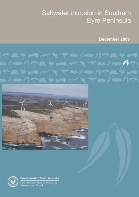
<strong>Saltwater</strong> <strong><strong>in</strong>trusion</strong> <strong>in</strong> <strong>Southern</strong><br />
<strong>Eyre</strong> Pen<strong>in</strong>sula<br />
<strong>December</strong> <strong>2009</strong><br />
i
This paper has been produced under the <strong>Eyre</strong> Pen<strong>in</strong>sula Hydrogeology Research Fellowship<br />
as a part of the <strong>Eyre</strong> Pen<strong>in</strong>sula Groundwater, Allocation and Plann<strong>in</strong>g Project.<br />
Authors: James Ward, Adrian Werner and Brenton Howe<br />
Date of publication: <strong>December</strong> <strong>2009</strong><br />
Front cover image: Sea cliffs and w<strong>in</strong>d farm near Uley South<br />
An appropriate citation for this report is:<br />
Ward, J.D., A.D. Werner and B. Howe <strong>2009</strong>, <strong>Saltwater</strong> Intrusion <strong>in</strong> <strong>Southern</strong> <strong>Eyre</strong> Pen<strong>in</strong>sula.<br />
Report developed through the <strong>Eyre</strong> Pen<strong>in</strong>sula Groundwater, Allocation and Plann<strong>in</strong>g Project.<br />
ii
Contents<br />
Executive Summary<br />
v<br />
1. Project Background 1<br />
1.1 <strong>Eyre</strong> Pen<strong>in</strong>sula Water Resources 1<br />
1.2 Report Context and the National Water Commission 2<br />
1.3 <strong>Eyre</strong> Pen<strong>in</strong>sula Hydrogeology Research Fellowship 3<br />
2. Introduction 4<br />
2.1 Broad EP Hydrogeology 4<br />
2.2 Significance of Seawater Intrusion on EP 6<br />
3. Past Investigations of Seawater Intrusion 8<br />
3.1 Monitor<strong>in</strong>g (drill<strong>in</strong>g and sond<strong>in</strong>g) 8<br />
3.2 Airborne Electromagnetic Survey 10<br />
3.3 Student Research Projects 13<br />
4. Methods 15<br />
4.1 Conceptual Models of Sal<strong>in</strong>e Intrusion 15<br />
4.1.1 General Concepts 15<br />
4.1.2 <strong>Eyre</strong> Pen<strong>in</strong>sula Examples 16<br />
4.2 Application of an Analytical Model 20<br />
4.2.1 Basic Model 20<br />
4.2.2 Dimensionless Formulation 22<br />
4.2.3 Steady-State Seawater Intrusion – Key Factors 24<br />
4.2.4 Steady-State Seawater Intrusion and Climate Change 25<br />
4.3 Parameterisation of EP Aquifers 26<br />
4.3.1 Aquifer Properties 26<br />
4.3.2 Regional Water Balance 28<br />
4.3.3 Inland Boundary Condition 28<br />
4.3.4 Parameter Summary 29<br />
4.3.5 Climate Change Scenarios 29<br />
5. Results and Discussion 30<br />
5.1 Seawater Intrusion Vulnerability of EP Aquifers 30<br />
5.2 Comparison with Observations 32<br />
5.2.1 Evidence of Up-con<strong>in</strong>g 32<br />
5.2.2 Depth to <strong>Saltwater</strong> Interface 33<br />
5.2.3 Sal<strong>in</strong>e Interface Predicted by AEM Survey 35<br />
5.3 Future Impacts 36<br />
5.3.1 Climate Change 36<br />
5.3.2 Increased Extraction 37<br />
5.4 Confidence <strong>in</strong> Predictions 39<br />
5.4.1 Uncerta<strong>in</strong>ty <strong>in</strong> Climate Change Scenarios 39<br />
5.4.2 Outstand<strong>in</strong>g Data Gaps 40<br />
6. Conclusions 41<br />
7. Future Work 42<br />
7.1 Ongo<strong>in</strong>g Work 42<br />
7.1.1 Monitor<strong>in</strong>g of <strong>Saltwater</strong> Interface <strong>in</strong> Coastal Wells 42<br />
7.1.2 Scenario Test<strong>in</strong>g Us<strong>in</strong>g a Numerical Model 42<br />
7.2 Suggested Further Work 43<br />
7.2.1 Investigation of Heterogeneity 43<br />
7.2.2 Investigation of Transient Behaviour and Reversibility 44<br />
7.2.3 Investigation <strong>in</strong>to <strong>Saltwater</strong> Up-con<strong>in</strong>g 44<br />
7.2.4 Uncerta<strong>in</strong>ty Analysis of Seawater Intrusion Approaches 44<br />
7.2.5 Assessment of Sources of Sal<strong>in</strong>ity 44<br />
References 45<br />
Appendix - Data and <strong>in</strong>terpretation provided by SA Water 48<br />
iii
Tables<br />
Table 1. Summary of hydrogeologic units ............................................................................5<br />
Table 2. Aquifer parameters adopted for analytical modell<strong>in</strong>g .............................................. 29<br />
Table 3. Dimensionless parameters for seawater <strong><strong>in</strong>trusion</strong> extent <strong>in</strong> <strong>Southern</strong><br />
Bas<strong>in</strong>s .......................................................................................................................... 30<br />
Figures<br />
Figure 1. Regional map show<strong>in</strong>g major groundwater resources on EP ..................................1<br />
Figure 2. <strong>Southern</strong> Bas<strong>in</strong>s PWA, show<strong>in</strong>g location of <strong>in</strong>dividual groundwater<br />
bas<strong>in</strong>s and SA Water production bores. ..........................................................................6<br />
Figure 3. Typical groundwater level trends <strong>in</strong> three coastal aquifers (Coff<strong>in</strong> Bay,<br />
Uley South and L<strong>in</strong>coln Bas<strong>in</strong>) and one <strong>in</strong>land aquifer (Uley Wanilla). .............................7<br />
Figure 4. Sal<strong>in</strong>ity profiles <strong>in</strong> coastal Uley South observation wells (both ~500m<br />
<strong>in</strong>land) ............................................................................................................................9<br />
Figure 5. Conductivity slice at -53m ADH, annotated features <strong>in</strong>clude resistive<br />
basement ridges (blue) and conductive sal<strong>in</strong>e groundwater (p<strong>in</strong>k/red) (After<br />
Fitzpatrick et al. <strong>2009</strong>). ................................................................................................ 11<br />
Figure 6. Conductivity slice at -23m AHD show<strong>in</strong>g potential small seawater<br />
wedge extend<strong>in</strong>g <strong>in</strong>land <strong>in</strong>to Uley South........................................................................ 12<br />
Figure 7. Interpreted surface for base of Bridgewater formation; annotation<br />
shows area below mean sea level. ............................................................................... 13<br />
Figure 8. Two Conceptual models for seawater <strong><strong>in</strong>trusion</strong> <strong>in</strong> Uley South Bas<strong>in</strong>. .................... 16<br />
Figure 9. Conceptual model of fresh/sal<strong>in</strong>e water <strong>in</strong>teractions <strong>in</strong> L<strong>in</strong>coln B Lens<br />
(above) and Coff<strong>in</strong> Bay (below). .................................................................................... 18<br />
Figure 10. Conceptual model for Robison Lens; pre and post pump<strong>in</strong>g (Brown<br />
and Harr<strong>in</strong>gton, 2003) .................................................................................................. 19<br />
Figure 11. Diagram of parameters for analytical model of seawater <strong><strong>in</strong>trusion</strong> ...................... 21<br />
Figure 12. Contours of x<br />
T<br />
for different M and F .................................................................. 25<br />
Figure 13. Contours of x<br />
T<br />
for: (a) Uley South (SE) – QL only, (b) Uley South<br />
(SE) – QL+TS, (c) Uley South (NW), (d) Coff<strong>in</strong> Bay A lens, (e) L<strong>in</strong>coln B<br />
lens. ............................................................................................................................. 31<br />
Figure 14. Evidence of seasonal sal<strong>in</strong>e up-con<strong>in</strong>g <strong>in</strong> L<strong>in</strong>coln B Lens. .................................. 32<br />
Figure 15. Plot of theoretical freshwater/saltwater <strong>in</strong>terface determ<strong>in</strong>ed from (2)<br />
for the southeast portion of Uley South, for the two conceptual models (QL<br />
only vs. QL + TS), show<strong>in</strong>g the approximate location and screened <strong>in</strong>terval<br />
of observation well SLE069. ........................................................................................ 34<br />
Figure 16. Plot of theoretical freshwater/saltwater <strong>in</strong>terface determ<strong>in</strong>ed from (2)<br />
for the northwest portion of Uley South assum<strong>in</strong>g a cont<strong>in</strong>uous clay aquitard<br />
at a depth of 15m. ........................................................................................................ 35<br />
Figure 17. Contours of x<br />
T<br />
across a range of climate change scenarios for the<br />
three aquifer conceptualisations <strong>in</strong> the Uley South bas<strong>in</strong>. .............................................. 37<br />
Figure 18. Basic assessment of steady-state seawater <strong><strong>in</strong>trusion</strong> extent under<br />
different <strong>in</strong>creased pump<strong>in</strong>g scenarios, assum<strong>in</strong>g a coastl<strong>in</strong>e width of 5km. .................. 38<br />
iv
Executive Summary<br />
The <strong>Eyre</strong> Pen<strong>in</strong>sula (EP) <strong>in</strong> South Australia is home to some 55,000 people, with an<br />
economy supported significantly by agriculture and aquaculture exports. A network of<br />
ma<strong>in</strong>s pipel<strong>in</strong>es covers much of the region with the majority of this water be<strong>in</strong>g used<br />
for domestic consumption and stock water<strong>in</strong>g. EP sources approximately 85% of its<br />
ma<strong>in</strong>s water from unconf<strong>in</strong>ed aquifers with<strong>in</strong> the Quaternary limestone (Bridgewater)<br />
formation, the most significant resource be<strong>in</strong>g the Uley South Bas<strong>in</strong> near the<br />
southern tip of the pen<strong>in</strong>sula. Regional groundwater levels are heavily <strong>in</strong>fluenced by<br />
seasonal recharge, however the aquifers typically exhibit low hydraulic gradients due<br />
to high hydraulic conductivities. Many of the aquifers on the southern EP are <strong>in</strong> direct<br />
hydraulic connection with the sea, and the low hydraulic heads suggest a potential<br />
seawater <strong><strong>in</strong>trusion</strong> threat, particularly dur<strong>in</strong>g periods of low recharge.<br />
This report utilises a simple analytical solution to model the flow of freshwater<br />
overly<strong>in</strong>g a stationary saltwater wedge adjacent to the sea. The steady-state model<br />
solves the <strong>in</strong>land extent of the wedge (reported as the toe of the freshwater-saltwater<br />
<strong>in</strong>terface) as a function of the aquifer properties and the rate of freshwater discharge<br />
to the sea; high discharge results <strong>in</strong> a saltwater wedge that is closer to the coast,<br />
whereas reductions <strong>in</strong> discharge (due to recharge decl<strong>in</strong>e and/or <strong>in</strong>creased<br />
extraction) lead to a landward shift <strong>in</strong> the saltwater wedge, i.e. seawater <strong><strong>in</strong>trusion</strong>.<br />
The model is presented as a useful “first step” to help build <strong>in</strong>tuition around some of<br />
the processes that <strong>in</strong>fluence the position of the saltwater wedge <strong>in</strong> the southern EP.<br />
Future efforts will move towards a numerical groundwater model for the Uley South<br />
bas<strong>in</strong> to provide for transient, spatially variable predictions of seawater <strong><strong>in</strong>trusion</strong>. The<br />
simplistic method adopted here provides only a prelim<strong>in</strong>ary assessment of seawater<br />
<strong><strong>in</strong>trusion</strong> <strong>in</strong> relative terms; three-dimensional numerical model<strong>in</strong>g is required to<br />
properly account for the complexities of the system and to allow for seawater<br />
<strong><strong>in</strong>trusion</strong> characterisation for the purposes of under-p<strong>in</strong>n<strong>in</strong>g water resources<br />
plann<strong>in</strong>g.<br />
The application of the analytical solution to steady-state seawater <strong><strong>in</strong>trusion</strong> broadly<br />
supports the f<strong>in</strong>d<strong>in</strong>gs of a recent Airborne Electromagnetic (AEM) survey, which<br />
<strong>in</strong>dicates that seawater generally extends only a limited distance (~500m) <strong>in</strong>to the<br />
Uley South Bas<strong>in</strong> (at the time of the survey <strong>in</strong> 2006). The AEM survey also identified<br />
a region of deep basement <strong>in</strong> the southeast portion of the bas<strong>in</strong> as hav<strong>in</strong>g a higher<br />
potential for seawater <strong><strong>in</strong>trusion</strong>. The analytical modell<strong>in</strong>g presented <strong>in</strong> this report has<br />
compared the different conditions found <strong>in</strong> different portions of Uley South. The<br />
model <strong>in</strong>dicates that there is an elevated risk <strong>in</strong> the southeast portion due to the<br />
relatively deep basement and the possible absence of a clay aquitard, while <strong>in</strong> other<br />
areas the presence of a clay aquitard underneath the Bridgewater Formation leads to<br />
a lower potential for seawater <strong><strong>in</strong>trusion</strong>. Note that <strong>in</strong>formation from a recent<br />
<strong>in</strong>vestigation relat<strong>in</strong>g to the presence of a clay aquitard (<strong>in</strong>clud<strong>in</strong>g <strong>in</strong> the southeast<br />
portion of Uley South) is conta<strong>in</strong>ed <strong>in</strong> the Appendix.<br />
The modell<strong>in</strong>g is extended to form a prelim<strong>in</strong>ary analysis of seawater <strong><strong>in</strong>trusion</strong> under<br />
changes <strong>in</strong> conditions (sea-level rise / recharge changes) as might be <strong>in</strong>duced under<br />
climate change scenarios. For Uley South, it is found that a possible future decl<strong>in</strong>e <strong>in</strong><br />
recharge is likely to contribute far more to the long-term seawater <strong><strong>in</strong>trusion</strong> threat<br />
v
than <strong>in</strong>creases <strong>in</strong> sea-level. This assumes that the aquifer water levels are allowed to<br />
rise at a similar rate to the rise <strong>in</strong> sea-level.<br />
Other groundwater resources on EP such as the Coff<strong>in</strong> Bay “A” and L<strong>in</strong>coln “B”<br />
Lenses are at risk of <strong><strong>in</strong>trusion</strong> via a different process - saltwater up-con<strong>in</strong>g. This<br />
mode of <strong><strong>in</strong>trusion</strong> is not <strong>in</strong>vestigated quantitatively <strong>in</strong> this study although up-con<strong>in</strong>g<br />
has been observed <strong>in</strong> both of these aquifers. It is therefore recommended that a<br />
study be undertaken <strong>in</strong>to the likely threat of up-con<strong>in</strong>g <strong>in</strong> those bas<strong>in</strong>s under present<br />
and possible future recharge and pump<strong>in</strong>g scenarios.<br />
To date, the threat of seawater <strong><strong>in</strong>trusion</strong> <strong>in</strong> the <strong>Southern</strong> Bas<strong>in</strong>s has not been studied<br />
thoroughly <strong>in</strong> the context of resource management. Groundwater extraction volumes<br />
have been set accord<strong>in</strong>g to historical recharge (“flux-based management”), despite<br />
fall<strong>in</strong>g trends <strong>in</strong> groundwater levels, and some very low water levels develop<strong>in</strong>g near<br />
the coast <strong>in</strong> places. The dynamic nature of the saltwater <strong>in</strong>terface needs to be<br />
<strong>in</strong>vestigated to properly assess seawater <strong><strong>in</strong>trusion</strong> under different management<br />
approaches. To achieve this, a more <strong>in</strong>-depth analysis of seawater <strong><strong>in</strong>trusion</strong> is<br />
required, <strong>in</strong>volv<strong>in</strong>g the application of numerical models that account for the 3D<br />
dispersive nature of the process.<br />
To improve confidence <strong>in</strong> the susta<strong>in</strong>able use of the groundwater resources there<br />
must be an <strong>in</strong>crease <strong>in</strong> the frequency of targeted monitor<strong>in</strong>g; <strong>in</strong> the higher-risk area <strong>in</strong><br />
the southeast of Uley South, sal<strong>in</strong>ity profiles for coastal wells have so far been<br />
obta<strong>in</strong>ed only twice s<strong>in</strong>ce 2004. There is a need for an improved understand<strong>in</strong>g of the<br />
movement of the freshwater/saltwater <strong>in</strong>terface over time, and preferably a l<strong>in</strong>k to<br />
more proactive (such as “trigger-level”) management styles that can encompass the<br />
dynamic nature of seawater <strong><strong>in</strong>trusion</strong> risk and ensure protection of these crucial<br />
groundwater resources.<br />
vi
1. Project Background<br />
1.1 <strong>Eyre</strong> Pen<strong>in</strong>sula Water Resources<br />
<strong>Eyre</strong> Pen<strong>in</strong>sula (EP) is a diverse region with extensive coastl<strong>in</strong>e, numerous native<br />
vegetation communities, various land uses and water systems and a Mediterraneantype<br />
climate rang<strong>in</strong>g from arid to temperate conditions. The economy is based on<br />
agriculture (traditionally gra<strong>in</strong> and wool), seafood (fish<strong>in</strong>g and aquaculture), tourism,<br />
m<strong>in</strong><strong>in</strong>g and m<strong>in</strong>eral process<strong>in</strong>g <strong>in</strong>dustries.<br />
Water resources are relatively scarce on EP and major groundwater resources are<br />
conf<strong>in</strong>ed to the south and west coasts (Figure 1). Cities, towns, and <strong>in</strong>dustry rely on<br />
potable ma<strong>in</strong>s (or reticulated) water provided by SA Water via an extensive network<br />
of pipel<strong>in</strong>es that cover much of the west and east coasts of the Pen<strong>in</strong>sula. The region<br />
is also home to some 1.6 million sheep and 25,000 cattle (ABS, 2008), which<br />
consume approximately the same volume of reticulated water as all domestic and<br />
<strong>in</strong>dustrial users comb<strong>in</strong>ed. The vast majority of ma<strong>in</strong>s water (~85%) is sourced from<br />
prescribed groundwater resources 1 which are shown <strong>in</strong> Figure 1. The susta<strong>in</strong>able<br />
management of these resources is the jo<strong>in</strong>t responsibility of the EP Natural<br />
Resources Management Board (EPNRM) and the Department of Water, Land and<br />
Biodiversity Conservation (DWLBC). In addition to groundwater, a small proportion of<br />
ma<strong>in</strong>s water (~15%) is supplied from the River Murray to the EP, via the Whyalla to<br />
Kimba pipel<strong>in</strong>e.<br />
Figure 1. Regional map show<strong>in</strong>g major groundwater resources on EP<br />
1 Prescribed resources are designated under the Natural Resources Management Act ( 2004)<br />
1
The security of public water supplies on <strong>Eyre</strong> Pen<strong>in</strong>sula is managed through the SA<br />
Water Long Term Plan 2 . Under a scenario of cont<strong>in</strong>ued population growth and<br />
subsequent demand <strong>in</strong>crease, augmentation of the exist<strong>in</strong>g groundwater based<br />
supply will be required. Desal<strong>in</strong>ation of seawater has been identified as the preferred<br />
supply augmentation option rather than draw<strong>in</strong>g further on the River Murray.<br />
However, given the extent of capital already <strong>in</strong>vested <strong>in</strong> <strong>in</strong>frastructure, the cont<strong>in</strong>ued<br />
use of groundwater resources is the preferred water source option (more cost<br />
effective and less energy <strong>in</strong>tensive). For this reason, the proportion of the public<br />
water supply be<strong>in</strong>g sourced from groundwater should cont<strong>in</strong>ue to be maximized.<br />
It is important that groundwater resources are managed to ensure their long term<br />
susta<strong>in</strong>able use and to protect the natural ecosystems that depend on them. This is<br />
particularly important as we face the considerable risk of a chang<strong>in</strong>g climate.<br />
Incorporat<strong>in</strong>g climate change <strong>in</strong>to the management of the region’s water resources is<br />
vital and requires the consideration of the vulnerability or resilience of each resource.<br />
1.2 Report Context and the National Water<br />
Commission<br />
In Prescribed Wells Areas (PWAs), groundwater use is currently managed by way of<br />
annual allocations under a Water Allocation Plan (WAP). When undertak<strong>in</strong>g its 5<br />
yearly review of the WAPs <strong>in</strong> 2006, EPNRM consulted the community, who<br />
expressed concern regard<strong>in</strong>g the susta<strong>in</strong>ability of the groundwater bas<strong>in</strong>s. Key<br />
issues <strong>in</strong>cluded (but were not limited to): the impacts of climate change, how much<br />
water the environment needs, the impact of vegetation on recharge and the risk of<br />
seawater <strong><strong>in</strong>trusion</strong>.<br />
In 2008, the EP Groundwater Allocation, Plann<strong>in</strong>g & Management (GAPM) Project<br />
was launched to attempt to address the community’s concerns. The National Water<br />
Commission (NWC) committed $700,000 over ~2 years and this was matched<br />
through cash and <strong>in</strong> k<strong>in</strong>d contributions from the state-based partners: Department of<br />
Water, Land and Biodiversity Conservation, SA Water Corporation and <strong>Eyre</strong><br />
Pen<strong>in</strong>sula Natural Resources Management Board.<br />
The ma<strong>in</strong> objective of the GAPM Project is to improve the scientific understand<strong>in</strong>g<br />
that underp<strong>in</strong>s the susta<strong>in</strong>able management of the groundwater resources. The<br />
project <strong>in</strong>volves a suite of detailed <strong>in</strong>vestigations, which are tied to report<strong>in</strong>g<br />
milestones as follows:<br />
2 “Meet<strong>in</strong>g Future Demand : SA Water's Long Term Plan for <strong>Eyre</strong> Region”, completed <strong>in</strong> November 2008 and<br />
accessible via the SA Water website (www.sawater.com.au)<br />
2
Milestones 1-3 Project management objectives<br />
Milestone 4<br />
Milestone 5<br />
Milestone 6<br />
Milestone 7<br />
Milestone 8<br />
Milestone 9<br />
A detailed review of the current monitor<strong>in</strong>g of the groundwater<br />
resources<br />
The assessment of the impacts of climate change on ra<strong>in</strong>fall recharge<br />
Investigat<strong>in</strong>g the impacts of extraction and reduced aquifer recharge<br />
on seawater/groundwater <strong>in</strong>teraction<br />
Investigat<strong>in</strong>g the relationship between soils, vegetation and recharge<br />
The mapp<strong>in</strong>g of water-dependent ecosystems and an assessment of<br />
their water requirements<br />
The preparation of conceptual groundwater models<br />
Milestone 10 The preparation of numerical groundwater models and predictive<br />
scenarios to <strong>in</strong>form future management and allocation of groundwater<br />
resources.<br />
The project will assist EPNRM to develop new WAPs that will <strong>in</strong>clude a much more<br />
detailed assessment of the capacity of the resources to meet the demands for water<br />
on a cont<strong>in</strong>u<strong>in</strong>g basis.<br />
This report aims to deliver on Milestone 6 of the GAPM project. This report presents<br />
a conceptual understand<strong>in</strong>g of the nature of seawater <strong><strong>in</strong>trusion</strong>, specific to aquifer<br />
conditions <strong>in</strong> EP. The likely impacts of <strong>in</strong>creased extraction, reduced recharge and<br />
sea level rise are explored us<strong>in</strong>g a simplified approach <strong>in</strong>volv<strong>in</strong>g analytical models.<br />
1.3 <strong>Eyre</strong> Pen<strong>in</strong>sula Hydrogeology Research<br />
Fellowship<br />
The <strong>Eyre</strong> Pen<strong>in</strong>sula Hydrogeology Research Fellowship (EPHRF) was established to<br />
create a focal po<strong>in</strong>t of expertise at Fl<strong>in</strong>ders University and to address key strategic<br />
research and <strong>in</strong>vestigation issues related to EP’s water resources. The Fellowship is<br />
driven by three <strong>in</strong>dustry partners: EPNRM, DWLBC and SA Water with further<br />
fund<strong>in</strong>g support from the Fl<strong>in</strong>ders Centre for Coastal and Catchment Environments<br />
(FR3CE) and the Centre for Groundwater Studies. The collaboration model is one<br />
where a postdoctoral research fellow has been the focal po<strong>in</strong>t of <strong>in</strong>teractions between<br />
a collective work<strong>in</strong>g team compris<strong>in</strong>g Fl<strong>in</strong>ders University students (at Honours,<br />
Masters and PhD levels), as well as academic staff and <strong>in</strong>dustry partner members.<br />
The broad research themes of the fellowship align closely with the report<strong>in</strong>g<br />
milestones of the NWC GAPM project.<br />
3
2. Introduction<br />
In coastal aquifers with a hydraulic connection to the sea, assessment of “susta<strong>in</strong>able<br />
yield” must consider both the quantity and the quality of extracted water. It is a<br />
common misconception that extraction can be susta<strong>in</strong>ed provided it does not exceed<br />
recharge; however this alone is not sufficient for susta<strong>in</strong><strong>in</strong>g acceptable water quality<br />
(e.g. low sal<strong>in</strong>ity). In order to prevent seawater advanc<strong>in</strong>g <strong>in</strong>land <strong>in</strong> a coastal aquifer,<br />
there must be an adequate discharge of fresh groundwater to the sea. This implies<br />
that withdrawals from the coastal aquifer must be substantially less than total<br />
recharge, and that a certa<strong>in</strong> quantity of fresh groundwater must therefore be<br />
“expended” (i.e. via ocean discharge) to ensure protection of the quality of the<br />
rema<strong>in</strong><strong>in</strong>g freshwater.<br />
Under possible scenarios of climate change, the seawater <strong><strong>in</strong>trusion</strong> threat could<br />
<strong>in</strong>crease <strong>in</strong> several dist<strong>in</strong>ct (though <strong>in</strong>terrelated) ways: (i) sea-level rise causes a<br />
greater hydraulic forc<strong>in</strong>g on the seaward boundary of the aquifer and drives seawater<br />
further <strong>in</strong>land; (ii) decl<strong>in</strong><strong>in</strong>g ra<strong>in</strong>fall leads to a reduction <strong>in</strong> recharge and thus a decl<strong>in</strong>e<br />
<strong>in</strong> discharge to the sea; (iii) pump<strong>in</strong>g <strong>in</strong>creases <strong>in</strong> response to a warmer and drier<br />
climate, reduc<strong>in</strong>g the net discharge to the sea. Note that the latter change (an<br />
<strong>in</strong>crease <strong>in</strong> pump<strong>in</strong>g) may also be anticipated due to ongo<strong>in</strong>g population and<br />
economic growth <strong>in</strong> the region, irrespective of climate change.<br />
2.1 Broad EP Hydrogeology<br />
The various hydrogeologic units are summarised <strong>in</strong> Table 1. More detailed<br />
descriptions of EP hydrogeology can be obta<strong>in</strong>ed from numerous <strong>in</strong>vestigative<br />
reports produced through the SA M<strong>in</strong>es and Energy Department. Barnett (1980)<br />
produced a useful bibliography of hydrogeology that can be used to locate early<br />
reports specific to each <strong>in</strong>dividual area.<br />
The primary target for reticulated public water supply is the Bridgewater Formation,<br />
an unconf<strong>in</strong>ed Quaternary Limestone aquifer. The aquifer occurs as isolated lenses<br />
with generally high yields and low sal<strong>in</strong>ity. Skeletal soils, surface calcrete, sparse<br />
(sometimes absent) vegetation, the presence of surface dissolution features and<br />
karst limestone all contribute to enhanced recharge. Groundwater levels <strong>in</strong> these<br />
aquifers typically rise rapidly <strong>in</strong> response to episodes of high ra<strong>in</strong>fall and decl<strong>in</strong>e<br />
dur<strong>in</strong>g extended dry periods.<br />
The secondary aquifer is the Wanilla Formation, a semi-conf<strong>in</strong>ed Tertiary Sand<br />
aquifer characterised by generally lower yields and more brackish water than <strong>in</strong> the<br />
Bridgewater Formation. The Tertiary sands are usually (but not always) overla<strong>in</strong> by a<br />
relatively th<strong>in</strong> Tertiary Clay (the Uley Formation) of low permeability. Hydraulic<br />
gradients between the aquifers are generally low, <strong>in</strong>dicat<strong>in</strong>g that extensive <strong>in</strong>ter-layer<br />
flows probably occur.<br />
4
Table 1. Summary of hydrogeologic units 3<br />
Era Unit, Lithology Hydrogeology<br />
Recent (Holocene)<br />
Ca<strong>in</strong>ozoic<br />
Coastal Dunes: F<strong>in</strong>e-gra<strong>in</strong>ed<br />
aeolianites, unconsolidated, actively<br />
mobile. Gra<strong>in</strong>s comprise calcite and<br />
shell fragments.<br />
Unconf<strong>in</strong>ed Aquifer: seasonal, small<br />
yield<strong>in</strong>g, th<strong>in</strong>, low sal<strong>in</strong>ity supplies<br />
located at the base of the mobile<br />
sand dune systems<br />
Quaternary<br />
(Pleistocene)<br />
Ca<strong>in</strong>ozoic<br />
Bridgewater Formation: Aeolianites, Unconf<strong>in</strong>ed Aquifer: generally low<br />
f<strong>in</strong>e to medium-gra<strong>in</strong>ed, cross bedded, sal<strong>in</strong>ity. Permeability ranges from<br />
weakly to moderately cemented, Gra<strong>in</strong>s low to very high. Hydraulic<br />
are calcite and shell fragments, ma<strong>in</strong>ly conductivity ranges typically up to<br />
0.1 - 1.5 mm. Generally calcrete at 1000 m/day. The usual target<br />
surface.<br />
aquifer for large water supplies on<br />
EP.<br />
Tertiary (Eocene)<br />
Ca<strong>in</strong>ozoic<br />
Wanilla, Poelpena, and Pid<strong>in</strong>ga<br />
Formations: Clays, sands (quartz) and<br />
gravels with th<strong>in</strong> lignite layers. Sand is<br />
generally f<strong>in</strong>e-gra<strong>in</strong>ed, less than 0.5<br />
mm, uncemented or weakly cemented.<br />
Semi-conf<strong>in</strong>ed to Conf<strong>in</strong>ed Aquifer:<br />
low to moderate permeability but<br />
with marked variations vertically and<br />
laterally. Sal<strong>in</strong>ity variable and<br />
generally higher that the overly<strong>in</strong>g<br />
unconf<strong>in</strong>ed aquifer.<br />
Jurassic<br />
Mesozoic<br />
Polda Formation: Sands (quartz), silts<br />
and clays. Sand gra<strong>in</strong>s usually less<br />
than 0.5 mm, occasionally up to 3 mm.<br />
Sediments generally carbonaceous and<br />
conta<strong>in</strong> lignite beds.<br />
Conf<strong>in</strong>ed Aquifer: very low<br />
permeability, high groundwater<br />
sal<strong>in</strong>ity generally exceed<strong>in</strong>g 14,000<br />
mg/L.<br />
Neo-Proterozoic<br />
Proterozoic<br />
Pre-Cambrian Basement: Schists,<br />
gneisses and quartzites <strong>in</strong>truded by<br />
granites and basic rocks. Deeply<br />
weathered <strong>in</strong> places.<br />
Semi-conf<strong>in</strong>ed to Conf<strong>in</strong>ed Aquifers:<br />
groundwater occurs <strong>in</strong> the<br />
weathered profile or with<strong>in</strong> the<br />
fracture spaces of these rocks.<br />
Sal<strong>in</strong>ity generally exceeds 7,000<br />
mg/L, occasionally lower.<br />
3 Table compiled by DWLBC (Fact Sheet #3)<br />
5
2.2 Significance of Seawater Intrusion on EP<br />
Several of EP’s most important groundwater sources occur <strong>in</strong> coastal sett<strong>in</strong>gs. These<br />
<strong>in</strong>clude the Uley South and L<strong>in</strong>coln Bas<strong>in</strong>s, which respectively provide ~70% and<br />
~10% of total reticulated water, as well as Coff<strong>in</strong> Bay “A” Lens which currently<br />
provides 100% of reticulated water to the township of Coff<strong>in</strong> Bay (i.e. an isolated<br />
supply system). These resources lie with<strong>in</strong> the <strong>Southern</strong> Bas<strong>in</strong>s PWA (Figure 2).<br />
Given the overall importance of these aquifers, it is important to understand and<br />
manage aga<strong>in</strong>st the risk of seawater <strong><strong>in</strong>trusion</strong> due to either climate change or overextraction.<br />
Figure 2. <strong>Southern</strong> Bas<strong>in</strong>s PWA, show<strong>in</strong>g locations of <strong>in</strong>dividual groundwater bas<strong>in</strong>s and SA<br />
Water production bores. Note that water is not extracted from all bas<strong>in</strong>s; however three of the<br />
key production areas (Uley South, L<strong>in</strong>coln and Coff<strong>in</strong> Bay A) are located adjacent to the<br />
coast.<br />
6
Water Level (m AHD)<br />
Water Level (m AHD)<br />
Water Level (m AHD)<br />
Water Level (m AHD)<br />
Hydrographs from the four key water supply areas <strong>in</strong> the <strong>Southern</strong> Bas<strong>in</strong>s are shown<br />
(Figure 2.1b) for comparison. Of the four areas shown, the three coastal aquifers<br />
(Coff<strong>in</strong> Bay, Uley South and L<strong>in</strong>coln B) currently have relatively steady water levels at<br />
around 1m AHD (i.e. 1m above mean sea level). Uley Wanilla is an <strong>in</strong>land system<br />
occurr<strong>in</strong>g at a higher elevation, and is not connected to the coast, however it is<br />
<strong>in</strong>cluded here to show the contrast <strong>in</strong> water level trends. The past two decades of<br />
below-average recharge 4 are likely to have contributed to the downwards trend <strong>in</strong><br />
Uley Wanilla (~4m drop over 20 years, and cont<strong>in</strong>u<strong>in</strong>g to fall). Meanwhile, the<br />
downward trend is far less pronounced <strong>in</strong> the three coastal zones, where there is a<br />
“boundary condition” of 0 m AHD imposed by the sea. In these areas a reduction <strong>in</strong><br />
recharge is likely to have led to a reduction <strong>in</strong> freshwater outflow to the sea. This can<br />
theoretically cause <strong>in</strong>land movement of the saltwater wedge, which serves as an<br />
<strong>in</strong>flow to the aquifer thereby help<strong>in</strong>g to “buffer” further water level decl<strong>in</strong>e. The extent<br />
of this effect is currently untested, and requires more sophisticated methods than<br />
those adopted here. It is clear from other studies of seawater <strong><strong>in</strong>trusion</strong> that stable<br />
groundwater levels do not necessarily <strong>in</strong>dicate a stabilised saltwater wedge, because<br />
of the difference <strong>in</strong> lag time between the watertable (e.g. days-months) and saltwater<br />
wedge (e.g. months-years) follow<strong>in</strong>g a change <strong>in</strong> the hydrological conditions (e.g.<br />
recharge, pump<strong>in</strong>g, etc). In coastal aquifers, stable water levels may appear to imply<br />
that an equilibrium between recharge and discharge has occurred and that the<br />
aquifer provides a sufficient supply of water <strong>in</strong> terms of quantity, however if seawater<br />
is <strong>in</strong>trud<strong>in</strong>g the aquifer from the coast, then water quality may be at risk.<br />
2<br />
Coff<strong>in</strong> Bay - LKW027<br />
73<br />
Uley Wanila - ULE007<br />
72<br />
1<br />
71<br />
70<br />
0<br />
69<br />
68<br />
67<br />
-1<br />
1960 1965 1970 1975 1980 1985 1990 1995 2000 2005 2010<br />
66<br />
1960 1965 1970 1975 1980 1985 1990 1995 2000 2005 2010<br />
5<br />
Uley South - ULE102<br />
2<br />
L<strong>in</strong>coln B Lens - SLE030<br />
4<br />
3<br />
1<br />
2<br />
0<br />
1<br />
0<br />
1960 1965 1970 1975 1980 1985 1990 1995 2000 2005 2010<br />
-1<br />
1960 1965 1970 1975 1980 1985 1990 1995 2000 2005 2010<br />
Figure 3. Typical groundwater level 5 trends <strong>in</strong> three coastal aquifers (Coff<strong>in</strong> Bay, Uley South<br />
and L<strong>in</strong>coln Bas<strong>in</strong>) and one <strong>in</strong>land aquifer (Uley Wanilla). Note the “levell<strong>in</strong>g off” of coastal<br />
water levels at around 1m AHD, while <strong>in</strong>land levels have cont<strong>in</strong>ued to drop.<br />
4<br />
Note that <strong>in</strong> the Uley Wanilla bas<strong>in</strong>, pump<strong>in</strong>g rates have been greatly reduced over the past two decades <strong>in</strong> an effort<br />
to arrest the decl<strong>in</strong>e <strong>in</strong> water levels. Despite these efforts, water levels have cont<strong>in</strong>ued to drop sharply relative to the<br />
long-term average. As the fall <strong>in</strong> water levels are not easily attributable to over-extraction, it is thoughts that a<br />
reduction <strong>in</strong> recharge has occurred.<br />
5<br />
Data obta<strong>in</strong>ed from “ObsWell”, Primary Industries and Resources SA (PIRSA) https://obswell.pir.sa.gov.au/<br />
7
3. Past Investigations of<br />
Seawater Intrusion<br />
Consideration of seawater <strong><strong>in</strong>trusion</strong> on the <strong>Eyre</strong> Pen<strong>in</strong>sula has predom<strong>in</strong>antly<br />
focused on Uley South due to the large volumes of water extracted and thus its<br />
overall importance to water supply. Morton and Steel (1968) noted the presence of<br />
coastal spr<strong>in</strong>gs at Shoal Po<strong>in</strong>t (Figure 2.1) and used what was thought to be a<br />
“conservative” value of hydraulic conductivity (0.011 cusecs/ft 2 , or ~300 m/d) to<br />
estimate an aquifer discharge to the coast of ~17 GL/a (roughly 20% of ra<strong>in</strong>fall).<br />
Barnett (1978) revised this estimate up to 30 GL/a and considered that 50% of this<br />
could be extracted without fear of seawater <strong><strong>in</strong>trusion</strong>, cit<strong>in</strong>g favorable basement<br />
configuration (slop<strong>in</strong>g up from the coast to a relative high po<strong>in</strong>t near the extraction<br />
area) as the key to the m<strong>in</strong>imal risk.<br />
Evans (1997) further revised the estimate of discharge to the sea, this time<br />
consider<strong>in</strong>g only the central portion of the bas<strong>in</strong> (where extraction was occurr<strong>in</strong>g at<br />
the time) and us<strong>in</strong>g the Ghyben-Herzberg pr<strong>in</strong>ciple to account for a sal<strong>in</strong>e wedge at<br />
the coastal boundary. Discharge through this portion of the bas<strong>in</strong> was calculated to<br />
be ~11GL/a prior to the <strong>in</strong>clusion of the saltwater wedge, which was found to reduce<br />
the discharge estimate to ~5GL/a. Evans also used pressure transducers to<br />
demonstrate that water levels <strong>in</strong> the Tertiary Sand aquifer respond to tidal<br />
fluctuations, confirm<strong>in</strong>g the strong hydraulic connection to the sea.<br />
3.1 Monitor<strong>in</strong>g (drill<strong>in</strong>g and sond<strong>in</strong>g)<br />
In response to expansion of the Uley South bore field and <strong>in</strong>creased extraction <strong>in</strong><br />
2000, monitor<strong>in</strong>g <strong>in</strong>frastructure was upgraded (Clarke et al., 2003; Clarke, 2005).<br />
This <strong>in</strong>volved the construction of two long screened coastal monitor<strong>in</strong>g wells, allow<strong>in</strong>g<br />
the direct measurement of a sal<strong>in</strong>e <strong>in</strong>terface by sal<strong>in</strong>ity profil<strong>in</strong>g (sond<strong>in</strong>g). In 2004,<br />
the first sond<strong>in</strong>g identified a relatively sharp <strong>in</strong>terface at approximately 24 and 17<br />
meters below sea level <strong>in</strong> ULE205 and SLE69 respectively (Figure 4).<br />
Sond<strong>in</strong>g of these two wells was conducted aga<strong>in</strong> <strong>in</strong> 2008, with the aim of observ<strong>in</strong>g<br />
any trend changes <strong>in</strong> the system. The results, however, have proven <strong>in</strong>conclusive<br />
due to the long gap between monitor<strong>in</strong>g and the unknown impacts of tidal fluctuations<br />
or dispersion of the <strong>in</strong>terface. Further, the approach to sampl<strong>in</strong>g the long-screen<br />
wells was not consistent <strong>in</strong> the 2004 and 2008 sonde profiles – further<br />
measurements are needed that adopt a consistent approach. The data may <strong>in</strong>dicate<br />
that there has been no significant change <strong>in</strong> the depth of the <strong>in</strong>terface between fresh<br />
and saltwater, although the nature of the mix<strong>in</strong>g zone may have changed <strong>in</strong> ULE205.<br />
Note that Clarke (2005) recommended monitor<strong>in</strong>g of the seawater-freshwater<br />
<strong>in</strong>terface via sond<strong>in</strong>g at <strong>in</strong>tervals of 2-3 months <strong>in</strong>itially. A more <strong>in</strong>tensive <strong>in</strong>terface<br />
monitor<strong>in</strong>g program is now be<strong>in</strong>g planned (see Section 7.1.1).<br />
8
Elevation m AHD<br />
Elevation m AHD<br />
ULE 205<br />
EC uS/cm<br />
-10000 0 10000 20000 30000 40000 50000 60000<br />
2<br />
SLE 69<br />
EC uS/cm<br />
-10000 0 10000 20000 30000 40000 50000 60000<br />
2<br />
0<br />
0<br />
-2<br />
-4<br />
Jun 2004<br />
Jul 2008<br />
-2<br />
-4<br />
Nov 2004<br />
Jul 2008<br />
-6<br />
-6<br />
-8<br />
-8<br />
-10<br />
-10<br />
-12<br />
-12<br />
-14<br />
-16<br />
-18<br />
-20<br />
-14<br />
-16<br />
-18<br />
-20<br />
Mixed Zone<br />
-22<br />
-24<br />
-26<br />
-28<br />
-30<br />
-32<br />
Mixed Zone<br />
-22<br />
-24<br />
-26<br />
-28<br />
-30<br />
-32<br />
Figure 4. Sal<strong>in</strong>ity profiles <strong>in</strong> coastal Uley South observation wells (both are approximately<br />
500m <strong>in</strong>land)<br />
The <strong>in</strong>terpretation of sal<strong>in</strong>ity profiles from fully slotted wells is complicated by the<br />
potential for significant movement of water with<strong>in</strong> the well itself (Shalev et al., <strong>2009</strong>).<br />
Due to density differences, the <strong>in</strong>teraction between freshwater and saltwater<br />
commonly creates strong vertical components of flow near the coast, and these are<br />
usually upwards near the <strong>in</strong>terface. This means that the level of the <strong>in</strong>terface <strong>in</strong> the<br />
well is not necessarily an accurate representation of the <strong>in</strong>terface <strong>in</strong> the aquifer.<br />
Dur<strong>in</strong>g <strong>2009</strong>, drill<strong>in</strong>g <strong>in</strong> coastal areas of Uley South was conducted to <strong>in</strong>stall<br />
additional monitor<strong>in</strong>g <strong>in</strong>frastructure and to assist <strong>in</strong> the “ground truth<strong>in</strong>g” of AEM data<br />
(see Section 3.2). SA Water funded drill<strong>in</strong>g at two locations <strong>in</strong> the northwestern<br />
coastal area of the bas<strong>in</strong> where previously very few wells have been drilled and<br />
hence understand<strong>in</strong>g has been poor. EPNRM, through the complementary state<br />
fund<strong>in</strong>g program, drilled two wells (ULE156 & ULE209) <strong>in</strong> a s<strong>in</strong>gle location <strong>in</strong> the<br />
southeastern coastal area (where Fitzpatrick et al., <strong>2009</strong>, identified an area<br />
“particularly susceptible to salt water <strong><strong>in</strong>trusion</strong>”). At the time of this report, SA Water<br />
drill<strong>in</strong>g operations had been postponed due to technical difficulties. ULE156 was<br />
drilled to basement and did not encounter any water of sal<strong>in</strong>ity resembl<strong>in</strong>g seawater,<br />
<strong>in</strong>dicat<strong>in</strong>g an absence of seawater <strong><strong>in</strong>trusion</strong> <strong>in</strong> that area (Evans et al. <strong>2009</strong>), although<br />
monitor<strong>in</strong>g is ongo<strong>in</strong>g.<br />
9
3.2 Airborne Electromagnetic Survey<br />
In 2006, an airborne electromagnetic (AEM) survey was conducted over an area that<br />
covers the Uley South and Coff<strong>in</strong> Bay A lenses, <strong>in</strong>clud<strong>in</strong>g the area between them<br />
under the Coff<strong>in</strong> Bay National Park, where access for drill<strong>in</strong>g is severely limited and<br />
few boreholes exist. The major purposes of the study were to help def<strong>in</strong>e the bounds<br />
of the aquifers (stratigraphy) and to def<strong>in</strong>e the extent of sal<strong>in</strong>e groundwater with<strong>in</strong> the<br />
aquifers. The follow<strong>in</strong>g section serves as a summary of the Airborne Electromagnetic<br />
project and results. For further detail please refer to the f<strong>in</strong>al report (Fitzpatrick et al.<br />
<strong>2009</strong>).<br />
The AEM method provides a non-<strong>in</strong>vasive technique that collects <strong>in</strong>formation about<br />
the conductivity (or <strong>in</strong>versely, the resistivity) of the sub-surface. Conductivity is<br />
primarily controlled by a comb<strong>in</strong>ation of the rock porosity and the properties of the<br />
groundwater (<strong>in</strong> particular the presence of salts). Conductivity is also commonly<br />
<strong>in</strong>fluenced by the degree of saturation and the presence of clay. In this survey, areas<br />
of suspected sal<strong>in</strong>e groundwater were considered relatively easy to identify as they<br />
exhibited extremely high conductivities (Fitzpatrick et al., <strong>2009</strong>).<br />
The raw conductivity data were manipulated us<strong>in</strong>g advanced process<strong>in</strong>g (<strong>in</strong>version)<br />
techniques, and plausible <strong>in</strong>terpretations were made for the base and thickness of<br />
the Quaternary Limestone aquifer and base and thickness of the comb<strong>in</strong>ed Tertiary<br />
Clay, Sand and weathered basement sequences. Results were constra<strong>in</strong>ed us<strong>in</strong>g<br />
exist<strong>in</strong>g stratigraphic logs and down-hole logg<strong>in</strong>g. Interpretations of aquifer bounds<br />
compared well with <strong>in</strong>terpretations made by bore-logs alone, <strong>in</strong>dicat<strong>in</strong>g that the<br />
technique provided a useful <strong>in</strong>sight <strong>in</strong> areas where bore logs are sparse or absent.<br />
Deeper sequences (basement topography) were def<strong>in</strong>ed with lower confidence and<br />
were not def<strong>in</strong>ed at all below highly sal<strong>in</strong>e water due to mask<strong>in</strong>g of the signal by the<br />
salt water.<br />
In the Coff<strong>in</strong> Bay National Park area, AEM results suggested the presence of highsal<strong>in</strong>ity<br />
groundwater (presumed to be seawater) at depth, extend<strong>in</strong>g from the<br />
southern coastl<strong>in</strong>e to Coff<strong>in</strong> Bay (Figure 5). Limited drill<strong>in</strong>g at two locations <strong>in</strong> the<br />
National Park confirmed the presence of a significant thickness (~40m) of freshwater<br />
overly<strong>in</strong>g this sal<strong>in</strong>e water (Smith et al. 2007). Results of the AEM and drill<strong>in</strong>g were<br />
used to determ<strong>in</strong>e an approximate depth to the freshwater/ saltwater <strong>in</strong>terface but<br />
could not accurately def<strong>in</strong>e the depth to basement. The AEM method struggled to<br />
resolve below the sal<strong>in</strong>e aquifer, and drill<strong>in</strong>g ceased at a depth of ~60m without<br />
encounter<strong>in</strong>g basement.<br />
10
Figure 5. Conductivity slice at -53m ADH, annotated features <strong>in</strong>clude resistive basement<br />
ridges (blue) and conductive sal<strong>in</strong>e groundwater (p<strong>in</strong>k/red) (from Fitzpatrick et al. <strong>2009</strong>).<br />
AEM results also h<strong>in</strong>ted at a sal<strong>in</strong>e water wedge extend<strong>in</strong>g a limited distance <strong>in</strong>land<br />
along the coast <strong>in</strong> Uley South (Figure 6). The high conductivity zones <strong>in</strong>terpreted and<br />
annotated as sal<strong>in</strong>e groundwater generally occur <strong>in</strong> the thick sedimentary “troughs’<br />
between basement ridges. Wells drilled to sufficient depth and completed with long<br />
screens (ULE205, SLE69) confirm the presence of seawater beneath freshwater and<br />
the two datasets provide reasonable agreement. The AEM survey <strong>in</strong>dicates (at least<br />
at the time of the survey <strong>in</strong> 2006) that seawater is likely to extend only a short<br />
distance, <strong>in</strong> the order of 500 metres <strong>in</strong>to the Uley South aquifer.<br />
11
Figure 6. Conductivity slice at -23m AHD show<strong>in</strong>g potential small seawater wedge extend<strong>in</strong>g<br />
<strong>in</strong>land <strong>in</strong>to Uley South. Note: miss<strong>in</strong>g data (white strip adjacent to the coast <strong>in</strong> the<br />
southeastern region) due to w<strong>in</strong>d farm along flight l<strong>in</strong>es (from Fitzpatrick et al. <strong>2009</strong>).<br />
The AEM survey also highlighted an area along the southeastern region of Uley<br />
South where the base of the Quaternary limestone aquifer appears to be a<br />
considerable thickness, possibly extend<strong>in</strong>g >30m below sea level (Figure 7). These<br />
areas present a higher risk for seawater <strong><strong>in</strong>trusion</strong>, and are <strong>in</strong> contrast to other areas<br />
where basement is much closer to sea-level (at several po<strong>in</strong>ts along the coast, the<br />
basement is even understood to be well above sea level, imply<strong>in</strong>g no direct<br />
connection to the sea <strong>in</strong> those locations). The southeastern area identified as highest<br />
risk for seawater <strong><strong>in</strong>trusion</strong> due to the comb<strong>in</strong>ation of deep basement, thick sediments<br />
and a th<strong>in</strong> or absent aquitard, is considered the most urgent area for targeted,<br />
ongo<strong>in</strong>g monitor<strong>in</strong>g.<br />
12
Figure 7. Interpreted surface for base of Bridgewater formation; annotation shows area below<br />
mean sea level (from Fitzpatrick et al. <strong>2009</strong>).<br />
3.3 Student Research Projects<br />
The EP Hydrogeology Fellowship (see Section 1.3) is mak<strong>in</strong>g progress towards the<br />
first body of research dedicated to seawater <strong><strong>in</strong>trusion</strong> on EP. A significant focus of<br />
this effort has been the tra<strong>in</strong><strong>in</strong>g of students at Honours level. Prior to the current<br />
report, two Honours theses have been written (Seidel, 2008; Alcoe, <strong>2009</strong>) relat<strong>in</strong>g to<br />
seawater <strong><strong>in</strong>trusion</strong> on EP.<br />
Seidel (2008) presented a simple assessment of seawater <strong><strong>in</strong>trusion</strong> and used<br />
steady-state analytical methods to <strong>in</strong>vestigate sensitivity of seawater <strong><strong>in</strong>trusion</strong><br />
extent to aquifer parameters and different conceptual models.<br />
Alcoe (<strong>2009</strong>) considered sal<strong>in</strong>e <strong><strong>in</strong>trusion</strong> the primary management risk <strong>in</strong> his<br />
parsimonious assessment of trigger-level management compared to the<br />
current flux-based management. A steady-state (monthly) water balance<br />
model <strong>in</strong>corporated both extent of seawater <strong>in</strong>cursion and volumes of<br />
seawater <strong>in</strong>to its framework.<br />
13
Research is cont<strong>in</strong>u<strong>in</strong>g under the EP Hydrogeology Fellowship, and at the time of<br />
prepar<strong>in</strong>g this report, a journal paper (Ward et al., In Prep.) has been simultaneously<br />
<strong>in</strong> preparation, consider<strong>in</strong>g climate change impacts on seawater <strong><strong>in</strong>trusion</strong>. The<br />
analytical methods used by Seidel (2008) and Alcoe (<strong>2009</strong>), which are extended <strong>in</strong><br />
Ward et al. (In Prep.), have formed the basis for the assessment method that is<br />
heavily relied upon <strong>in</strong> subsequent sections of this report. While the method is applied<br />
here for several idealized EP aquifer sett<strong>in</strong>gs, it is also used by Ward et al., (In Prep.)<br />
to ga<strong>in</strong> more generalized <strong>in</strong>sights <strong>in</strong>to the driv<strong>in</strong>g factors beh<strong>in</strong>d seawater <strong><strong>in</strong>trusion</strong><br />
impacts under comb<strong>in</strong>ed recharge decl<strong>in</strong>e and sea-level rise. This builds<br />
substantially on the <strong>in</strong>ternational literature, <strong>in</strong> which the impact of sea-level rise on<br />
seawater <strong><strong>in</strong>trusion</strong> has been generally studied (e.g. Werner and Simmons, <strong>2009</strong>), but<br />
generalized studies of the possible impacts of decl<strong>in</strong><strong>in</strong>g recharge have not been<br />
done.<br />
14
4. Methods<br />
Ow<strong>in</strong>g to the very high proportion of groundwater that cont<strong>in</strong>ues to be supplied by<br />
Uley South and the close proximity of the bas<strong>in</strong> to the sea, this study will focus on the<br />
potential threats to this system from seawater <strong><strong>in</strong>trusion</strong>. This means that the<br />
analytical solution employed is for the impermeable basement conceptual model<br />
described above. The issue of saltwater up-con<strong>in</strong>g under Coff<strong>in</strong> Bay or L<strong>in</strong>coln Bas<strong>in</strong><br />
will not be quantitatively <strong>in</strong>vestigated <strong>in</strong> this study but will be <strong>in</strong>vestigated qualitatively<br />
based on observations of well sal<strong>in</strong>ity. It is recommended that a more quantitative<br />
analysis of the up-con<strong>in</strong>g risk <strong>in</strong> those bas<strong>in</strong>s be conducted under possible future<br />
works.<br />
4.1 Conceptual Models of Sal<strong>in</strong>e Intrusion<br />
4.1.1 General Concepts<br />
A fundamental aspect of the <strong>in</strong>teraction between freshwater and saltwater is the<br />
density difference present between the fluids (i.e. seawater is denser than<br />
freshwater). Some level of mix<strong>in</strong>g between the fluids usually occurs, the extent of<br />
which is dictated by heterogeneity of aquifer properties and time-vary<strong>in</strong>g flow<br />
processes (e.g. recharge, tides). However, provided relatively stable conditions are<br />
present there is a tendency for freshwater to stratify above saltwater.<br />
Several different conceptual models for the saltwater/freshwater <strong>in</strong>teractions are<br />
applicable to the different aquifer sett<strong>in</strong>gs on EP. We will make a dist<strong>in</strong>ction here<br />
between “lateral seawater <strong><strong>in</strong>trusion</strong>” and “saltwater up-con<strong>in</strong>g”, with each term be<strong>in</strong>g<br />
def<strong>in</strong>ed below. The two different concepts require the application of different<br />
analytical models 6 and are likely to result <strong>in</strong> different extraction management and<br />
monitor<strong>in</strong>g targets.<br />
Lateral seawater <strong><strong>in</strong>trusion</strong> is likely to occur as a result of over-extraction (the most<br />
commonly considered case), but could also be caused by a decrease <strong>in</strong> recharge, or<br />
sea-level rise. In other words, it is caused by a disruption of the hydraulic equilibrium<br />
of the coastal groundwater system. If the equilibrium is disturbed, e.g. due to<br />
extraction, the <strong>in</strong>terface will move <strong>in</strong>land toward the po<strong>in</strong>t of extraction. Seawater<br />
<strong><strong>in</strong>trusion</strong> typically takes the form of a “wedge” of saltwater underly<strong>in</strong>g the discharg<strong>in</strong>g<br />
freshwater (Figure 8), hence seawater <strong><strong>in</strong>trusion</strong> moves furthest at the base of the<br />
aquifer. Analytical models can be used to predict the position of the wedge ”toe” (the<br />
<strong>in</strong>land tip of the wedge), which can be used to assist management decisions. If the<br />
toe <strong>in</strong>trudes <strong>in</strong>land past the location of production bores but the freshwater-saltwater<br />
<strong>in</strong>terface rema<strong>in</strong>s well below the production bore screen, saltwater up-con<strong>in</strong>g may<br />
become a more significant threat.<br />
<strong>Saltwater</strong> up-con<strong>in</strong>g has the potential to occur when freshwater is extracted from a<br />
fresh groundwater body that is underla<strong>in</strong> by sal<strong>in</strong>e water (Dagan and Bear, 1968;<br />
Reilly and Goodman, 1987). If extraction results <strong>in</strong> an upward vertical gradient<br />
sufficient to overcome the density-<strong>in</strong>duced stratification, it creates the potential for<br />
6<br />
The analytical methods described later <strong>in</strong> this report (section 3.1) do not apply to the saltwater up-con<strong>in</strong>g concept<br />
15
upward flow of sal<strong>in</strong>e water <strong>in</strong>to the production well. Broadly speak<strong>in</strong>g, the greater<br />
the drawdown at the po<strong>in</strong>t of extraction, the greater the potential for up-con<strong>in</strong>g.<br />
<strong>Saltwater</strong> up-con<strong>in</strong>g can potentially occur relatively quickly, and – depend<strong>in</strong>g on the<br />
particular comb<strong>in</strong>ation of aquifer properties and extraction rates – may possibly lead<br />
to anyth<strong>in</strong>g from a widespread rise <strong>in</strong> the sal<strong>in</strong>e <strong>in</strong>terface to a highly localized<br />
upwell<strong>in</strong>g immediately around the po<strong>in</strong>t of over-extraction. The processes,<br />
timeframes and reversibility of saltwater up-con<strong>in</strong>g are not well understood <strong>in</strong> a<br />
fundamental way, and research <strong>in</strong> this field is ongo<strong>in</strong>g (e.g. Werner et al., <strong>2009</strong>).<br />
4.1.2 <strong>Eyre</strong> Pen<strong>in</strong>sula Examples<br />
Several examples of different aquifer sett<strong>in</strong>gs, and the likely resultant <strong>in</strong>teraction<br />
between fresh and saltwater are presented below with reference to specific EP<br />
cases.<br />
Aquifer underla<strong>in</strong> by an impermeable basement<br />
In this conceptual model the coastal aquifer is considered to be underla<strong>in</strong> by a<br />
cont<strong>in</strong>uous, completely impermeable medium. For example, two similar variations of<br />
this concept exist <strong>in</strong> Uley South (Figure 8). In some areas of Uley South (“clay<br />
present”) the Bridgewater Formation is underla<strong>in</strong> by the Uley Formation Tertiary Clay<br />
which is presumed here to be impermeable for the purposes of apply<strong>in</strong>g the<br />
analytical solution. In other areas (“clay absent”), the clay is absent and the regional<br />
basement complex acts as the impermeable basement. Both variations of this<br />
conceptual model will be explored <strong>in</strong> more detail us<strong>in</strong>g analytical methods later <strong>in</strong> this<br />
report.<br />
Figure 8. Two Conceptual models for seawater <strong><strong>in</strong>trusion</strong> <strong>in</strong> Uley South Bas<strong>in</strong>.<br />
16
On EP, seawater <strong><strong>in</strong>trusion</strong> <strong>in</strong> unconf<strong>in</strong>ed aquifers underla<strong>in</strong> by an impermeable<br />
basement or aquitard broadly present <strong>in</strong> the follow<strong>in</strong>g manner:<br />
- Solution features and other surface features has lead to enhanced recharge<br />
to upper aquifer<br />
- Fresh groundwater discharges to the coast<br />
- Aquitard is sometimes present and conf<strong>in</strong><strong>in</strong>g, sometimes absent.<br />
- Undulat<strong>in</strong>g impermeable crystall<strong>in</strong>e basement underlies the aquifers<br />
- Under steady-state conditions, a sal<strong>in</strong>e wedge exists that is held <strong>in</strong> place by<br />
freshwater discharge to the sea<br />
- Over-extraction and/or decl<strong>in</strong><strong>in</strong>g recharge will reduce discharge to the sea,<br />
caus<strong>in</strong>g the “toe” of the <strong>in</strong>terface to migrate towards a new steady-state<br />
position further <strong>in</strong>land.<br />
- An <strong>in</strong>crease <strong>in</strong> sea-level creates a larger saltwater head at the coast, and<br />
without an <strong>in</strong>crease <strong>in</strong> discharge this will force the wedge to tend towards a<br />
new steady-state position further <strong>in</strong>land<br />
Coastal freshwater lens<br />
In cases where the basement is sufficiently deep, it is possible for the saltwater to<br />
completely underlie the freshwater body but does not necessarily contam<strong>in</strong>ate<br />
shallow pump<strong>in</strong>g wells (e.g. Coff<strong>in</strong> Bay A Lens, L<strong>in</strong>coln B Lens). This results <strong>in</strong> the<br />
fresh groundwater behav<strong>in</strong>g like a stratified layer (i.e. lens) overly<strong>in</strong>g seawater. On<br />
EP, these systems broadly present as follows:<br />
- Fresh groundwater discharges to the coast<br />
- Semi permeable clay layer (not shown) is present <strong>in</strong> some areas, help<strong>in</strong>g to<br />
separate waters of different quality<br />
- Denser sal<strong>in</strong>e groundwater (maybe seawater) underlies most or all of the<br />
fresh groundwater and is closest to the surface near the coast<br />
- Extraction leads to a local depression <strong>in</strong> water table, <strong>in</strong>duc<strong>in</strong>g lateral and<br />
upward groundwater flow<br />
- <strong>Saltwater</strong> up-con<strong>in</strong>g occurs below the po<strong>in</strong>t of extraction; the speed and<br />
severity is l<strong>in</strong>ked to the thickness of freshwater between the bottom of the<br />
production zone and the freshwater-saltwater <strong>in</strong>terface.<br />
17
Figure 9. Conceptual model of fresh/sal<strong>in</strong>e water <strong>in</strong>teractions <strong>in</strong> L<strong>in</strong>coln B Lens (above) and<br />
Coff<strong>in</strong> Bay (below).<br />
Observations and further discussion of saltwater up-con<strong>in</strong>g <strong>in</strong> L<strong>in</strong>coln B and Coff<strong>in</strong><br />
Bay A are provided <strong>in</strong> Section 5.2.1.<br />
18
Inland freshwater lens<br />
It is worth not<strong>in</strong>g that sal<strong>in</strong>e <strong><strong>in</strong>trusion</strong> can also occur <strong>in</strong> <strong>in</strong>land aquifers that are<br />
disconnected from the coast. In certa<strong>in</strong> situations, a freshwater lens may reside over<br />
brackish or sal<strong>in</strong>e groundwater (e.g. Rob<strong>in</strong>son Lens). This is conceptually different to<br />
a coastal lens where the underly<strong>in</strong>g sal<strong>in</strong>e water is seawater (due to hydraulic<br />
connection with the coast), although similar pr<strong>in</strong>ciples apply <strong>in</strong> regards to density<br />
effects, saltwater stratification and up-con<strong>in</strong>g. Figure 10 shows an example for the<br />
Rob<strong>in</strong>son lens on EP presented by Brown and Harr<strong>in</strong>gton (2003). The Rob<strong>in</strong>son lens<br />
can be broadly described as follows:<br />
- Formation of lens due to preferential recharge via solution features.<br />
- Displacement of higher sal<strong>in</strong>ity water and some freshwater-saltwater mix<strong>in</strong>g<br />
- Presence of semi permeable clay layer (not shown) helps to separate waters<br />
of different quality<br />
- Deep rooted trees access fresh/brackish groundwater (shown <strong>in</strong> Figure 10 for<br />
Rob<strong>in</strong>son Lens)<br />
- Extraction depletes freshwater reserves and causes saltwater up-con<strong>in</strong>g at<br />
the po<strong>in</strong>t of extraction<br />
- Small reserves of freshwater may still be present but cannot be accessed<br />
us<strong>in</strong>g exist<strong>in</strong>g <strong>in</strong>frastructure<br />
Figure 10. Conceptual model for Robison Lens; pre and post pump<strong>in</strong>g (Brown and<br />
Harr<strong>in</strong>gton, 2003)<br />
19
4.2 Application of an Analytical Model<br />
The follow<strong>in</strong>g sections outl<strong>in</strong>e an analytical method for rapid and simplified<br />
assessment of vulnerability to seawater <strong><strong>in</strong>trusion</strong>, especially under scenarios of<br />
climate change. Analytical modell<strong>in</strong>g can be considered a “bare m<strong>in</strong>imum” approach<br />
to the characterization of coastal aquifers for seawater <strong><strong>in</strong>trusion</strong> studies, represent<strong>in</strong>g<br />
a useful start<strong>in</strong>g po<strong>in</strong>t before one undertakes more detailed analyses such as<br />
numerical modell<strong>in</strong>g. Furthermore, the rapid assessment of seawater <strong><strong>in</strong>trusion</strong> us<strong>in</strong>g<br />
analytical approaches allows one to prioritise data collection and modell<strong>in</strong>g efforts.<br />
This work draws heavily on journal paper content from Ward et al. (In Prep.), which<br />
has been produced under the Fellowship. Full derivations of the analytical solutions<br />
are covered <strong>in</strong> the journal paper.<br />
4.2.1 Basic Model<br />
Follow<strong>in</strong>g Werner and Simmons (<strong>2009</strong>), we adopt a steady-state, sharp-<strong>in</strong>terface<br />
analytical solution. Figure 11 shows a cross-sectional representation of flow to the<br />
coast, as adopted by previous studies (e.g. Strack, 1976, 1989; Naji et al., 1998;<br />
Mantoglou, 2003; Werner and Simmons, <strong>2009</strong>). The situation is an unconf<strong>in</strong>ed<br />
coastal aquifer, bounded below by an impervious horizontal layer at a depth B [L]<br />
below sea level. The <strong>in</strong>land distance x i [L] represents the coastal fr<strong>in</strong>ge, with any<br />
pump<strong>in</strong>g activities presumed to occur <strong>in</strong>land of x i . x i is expected to be on the order of<br />
several hundred to a few thousand metres and would be chosen such that it is of a<br />
scale relevant to plann<strong>in</strong>g – e.g. the maximum allowable seawater <strong><strong>in</strong>trusion</strong> extent.<br />
The aquifer is assumed to receive uniform recharge R [L/T] <strong>in</strong> the coastal fr<strong>in</strong>ge. Note<br />
that R is net recharge, after consider<strong>in</strong>g losses due to evapotranspiration from the<br />
water table. It is assumed that R ≥ 0. The system receives a lateral <strong>in</strong>flow q i [L 2 /T]<br />
through the <strong>in</strong>land boundary. q i may be considered to be the result of net recharge,<br />
account<strong>in</strong>g for losses due to pump<strong>in</strong>g <strong>in</strong>land from x i . The discharge q o [L 2 /T] of<br />
freshwater to the ocean is equal to the sum of the <strong>in</strong>flows (Rx i + q i ).<br />
As a result of the density contrast between freshwater and seawater, a wedge of<br />
dense seawater penetrates the coastal region of the aquifer, held <strong>in</strong> place by the<br />
discharge q o . In this model, the wedge is assumed to be def<strong>in</strong>ed by a sharp <strong>in</strong>terface.<br />
The depth of the <strong>in</strong>terface below sea-level is denoted d [L] and the wedge penetrates<br />
<strong>in</strong>land to a maximum distance x T [L].<br />
20
Figure 11. Diagram of parameters for analytical model of seawater <strong><strong>in</strong>trusion</strong><br />
The freshwater-saltwater <strong>in</strong>terface is assumed to <strong>in</strong>tercept the coastl<strong>in</strong>e (x = 0) at sea<br />
level, while <strong>in</strong> reality the <strong>in</strong>terface must be slightly below sea level at the coast, to<br />
allow freshwater to discharge. This assumption has little impact on the <strong>in</strong>terface toe<br />
length x T (Custodio, 1987; Cheng and Ouazar, 1999). x T is commonly adopted as a<br />
means of characteris<strong>in</strong>g the extent of seawater <strong><strong>in</strong>trusion</strong> (e.g. Naji et al., 1998;<br />
Cheng et al., 2000; Werner and Simmons, <strong>2009</strong>), and is found us<strong>in</strong>g the s<strong>in</strong>gle<br />
potential method (Strack, 1976; Mantoglou, 2003). Thus x T is given by:<br />
x<br />
q<br />
Rx<br />
R<br />
q<br />
Rx<br />
R<br />
K<br />
R<br />
2<br />
i i<br />
i i<br />
2<br />
T<br />
1 B<br />
(1)<br />
2<br />
where the density difference ratio<br />
s<br />
f<br />
seawater and freshwater densities [M/L 3 ].<br />
f<br />
, and where<br />
s<br />
and<br />
f<br />
are respectively<br />
While x T is useful for characteris<strong>in</strong>g seawater <strong><strong>in</strong>trusion</strong> extent, it is not readily<br />
measurable <strong>in</strong> the field. The most common measurement <strong>in</strong> seawater <strong><strong>in</strong>trusion</strong><br />
monitor<strong>in</strong>g is the depth to the freshwater-saltwater <strong>in</strong>terface, which is found by<br />
sond<strong>in</strong>g (see Figure 4). The s<strong>in</strong>gle potential method can also be used to determ<strong>in</strong>e<br />
the depth d [L] to the <strong>in</strong>terface at a distance x from the coast, after Mantoglou (2003):<br />
d<br />
2x<br />
q<br />
i<br />
K<br />
R<br />
1<br />
x<br />
i<br />
x<br />
2<br />
(2)<br />
If the depth to the freshwater-saltwater <strong>in</strong>terface is known from field measurements,<br />
then d calculated from (2) could be used to <strong>in</strong>fer the <strong>in</strong>land extent and distribution of<br />
the freshwater-saltwater <strong>in</strong>terface. If sufficient <strong>in</strong>terface measurements are available<br />
along a transect, it may be possible to crudely calibrate the other parameters <strong>in</strong> the<br />
analytical model, or (perhaps more likely) to broadly cross-check the validity of the<br />
analytical solution.<br />
It should be noted that <strong>in</strong> their sea-level rise study, Werner and Simmons (<strong>2009</strong>)<br />
identified two different <strong>in</strong>land boundary conditions as end-members to the types of<br />
21
conditions expected <strong>in</strong> field sett<strong>in</strong>gs – a ”flux-controlled case”, and a ”head-controlled<br />
case”. Head-controlled boundaries may arise <strong>in</strong> situations where, for <strong>in</strong>stance, an<br />
<strong>in</strong>land water body (e.g. a canal, lake or wetland) of constant head occurs at the<br />
<strong>in</strong>land boundary of the model (e.g. <strong>in</strong> the case considered by Dausman and<br />
Langev<strong>in</strong>, 2005), or where pump<strong>in</strong>g occurs such that the <strong>in</strong>land head is constant<br />
despite sea-level rise. In Ward et al. (In Prep.), both flux-controlled and headcontrolled<br />
sett<strong>in</strong>gs are <strong>in</strong>vestigated further, however for the present study the fluxcontrolled<br />
boundary is considered to be the only relevant <strong>in</strong>land boundary condition.<br />
4.2.2 Dimensionless Formulation<br />
Naji et al. (1998) presented (1) <strong>in</strong> dimensionless form, and we adopt a similar form.<br />
The dimensionless clusters used below are slightly different to those of Naji et al.<br />
(1998) because they allow the physical processes to be described <strong>in</strong> terms of<br />
mean<strong>in</strong>gful ratios of the different flow types (as described below). The dimensionless<br />
seawater <strong><strong>in</strong>trusion</strong> extent is def<strong>in</strong>ed as<br />
x<br />
T<br />
x<br />
T<br />
(3)<br />
xi<br />
2<br />
such that: x T<br />
F 1 F 1 M F 1<br />
(4)<br />
where:<br />
q<br />
Rx<br />
i<br />
F ,<br />
i<br />
M<br />
K<br />
x<br />
i<br />
1<br />
q<br />
i<br />
B<br />
Rx<br />
i<br />
2<br />
(5)<br />
Here x<br />
T<br />
is the seawater <strong><strong>in</strong>trusion</strong> extent, expressed as a proportion of the <strong>in</strong>land<br />
distance x i . F and M are two dimensionless ratios describ<strong>in</strong>g the govern<strong>in</strong>g physical<br />
controls. F is the ratio of lateral <strong>in</strong>flow to coastal ra<strong>in</strong>fall-recharge (which we term<br />
“mixed <strong>in</strong>flow ratio” from here<strong>in</strong>). M is a ratio of free-convective components to<br />
forced-convective (advective) components that we term a “mixed convection ratio”, <strong>in</strong><br />
a similar fashion to Massmann et al. (2006) and Ward et al. (2007). In M, the<br />
numerator lumps together those parameters which we know contribute to <strong>in</strong>creas<strong>in</strong>g<br />
seawater <strong><strong>in</strong>trusion</strong> (most significantly K and B, as the density ratio is relatively<br />
constant for freshwater/seawater <strong>in</strong>teractions). The denom<strong>in</strong>ator <strong>in</strong> M conta<strong>in</strong>s the<br />
summed <strong>in</strong>flows, i.e. the discharge to the sea (which leads to the retardation of<br />
seawater <strong><strong>in</strong>trusion</strong>). The reason for us<strong>in</strong>g a dimensionless formulation is to reduce<br />
the number of critical parameters, so as to allow different systems to be more rapidly<br />
compared aga<strong>in</strong>st each other. In this case, all of the hydrogeological variables have<br />
been reduced to just two parameters (M and F), and as a result the idealised<br />
seawater <strong><strong>in</strong>trusion</strong> extent can be rapidly compared across multiple unconf<strong>in</strong>ed<br />
coastal aquifer systems which vary widely <strong>in</strong> terms of recharge and <strong>in</strong>land <strong>in</strong>flows,<br />
hydraulic conductivity, thickness and <strong>in</strong>land extent, by simply compar<strong>in</strong>g their<br />
respective M and F values.<br />
Mathematically, x<br />
T<br />
is def<strong>in</strong>ed over the <strong>in</strong>terval 0 M F 1 . What this means <strong>in</strong><br />
practical terms is that when M > F + 1 it implies that the toe of the wedge has<br />
<strong>in</strong>truded <strong>in</strong>land of the po<strong>in</strong>t of maximum hydraulic head (the peak of the coastal<br />
groundwater mound), and the situation becomes unstable (Strack, 1989).<br />
22
A Note on Analytical vs Numerical Modell<strong>in</strong>g<br />
A numerical model of the Uley South / Uley Bas<strong>in</strong>s is be<strong>in</strong>g constructed as part of the<br />
GAPM Project (Milestone 10), however <strong>in</strong> this report we seek to explore the factors that<br />
are likely to govern seawater <strong><strong>in</strong>trusion</strong> on <strong>Eyre</strong> Pen<strong>in</strong>sula fundamentally us<strong>in</strong>g<br />
analytical solutions. The follow<strong>in</strong>g discussion explores the fundamental differences<br />
between analytical and numerical modell<strong>in</strong>g and the benefits that both offer.<br />
The methods for modell<strong>in</strong>g groundwater systems can broadly be divided <strong>in</strong>to two classes:<br />
analytical and numerical. Analytical methods typically <strong>in</strong>volve an equation (or set of<br />
equations) describ<strong>in</strong>g a whole doma<strong>in</strong> (e.g. the depth to the freshwater-saltwater <strong>in</strong>terface<br />
be<strong>in</strong>g represented as a mathematical function of the distance <strong>in</strong>land). Numerical methods<br />
typically <strong>in</strong>volve divid<strong>in</strong>g the doma<strong>in</strong> <strong>in</strong>to smaller parts which are solved one-by-one and then<br />
reassembled <strong>in</strong>to a cohesive whole.<br />
The key advantage of analytical modell<strong>in</strong>g over numerical modell<strong>in</strong>g is that the former is very<br />
fast to construct and execute – a basic analytical model of a seawater <strong><strong>in</strong>trusion</strong> <strong>in</strong>terface may<br />
be developed from first pr<strong>in</strong>ciples <strong>in</strong> a matter of m<strong>in</strong>utes and then yields an answer <strong>in</strong> a matter<br />
of seconds. Def<strong>in</strong><strong>in</strong>g a problem <strong>in</strong> a s<strong>in</strong>gle set of equations also allows one to obta<strong>in</strong> explicit<br />
parameter group<strong>in</strong>gs that can be used to broadly characterise the underly<strong>in</strong>g physics<br />
govern<strong>in</strong>g system behaviour, for example the relationships between K, B, R and x T can be<br />
obta<strong>in</strong>ed with relative ease.<br />
On the other hand, analytical modell<strong>in</strong>g requires certa<strong>in</strong> elements of the conceptual model to<br />
be heavily constra<strong>in</strong>ed: for example, often the aquifer must be assumed homogeneous and<br />
the <strong>in</strong>terface must be assumed to be sharp (no dispersive mix<strong>in</strong>g). Moreover, analytical<br />
solutions to seawater <strong><strong>in</strong>trusion</strong> problems are usually steady-state and therefore cannot be<br />
used to simulate transient changes <strong>in</strong> conditions (such as the tim<strong>in</strong>g of the response to<br />
specific changes <strong>in</strong> recharge or sea-level, or different transient pump<strong>in</strong>g regimes).<br />
Numerical models, while more time-consum<strong>in</strong>g than analytical solutions, offer far greater<br />
flexibility as each discretized “cell” can be assigned <strong>in</strong>dividual properties, mak<strong>in</strong>g it possible to<br />
simulate different geological zones (heterogeneity). Furthermore, numerical solutions typically<br />
have a transient formulation, allow<strong>in</strong>g simulation of chang<strong>in</strong>g conditions over time, so that<br />
aspects of time scales, reversibility and remediation can be <strong>in</strong>vestigated. Numerical models<br />
can readily be established <strong>in</strong> 3-D and for complex aquifer geometries, mak<strong>in</strong>g them an<br />
attractive tool <strong>in</strong> bas<strong>in</strong> management.<br />
It must be remembered that a model can only ever be as reliable as the parameters used to<br />
construct, calibrate and validate it. In hydrogeology, parameter measurement almost always<br />
carries substantial uncerta<strong>in</strong>ty. Furthermore, a highly complex model with many “calibrateable”<br />
parameters may yield an excellent fit to the relatively small number of observations used<br />
to calibrate it, but may actually be less accurate between those po<strong>in</strong>ts (Hill, 2006).<br />
It is thus useful to approach modell<strong>in</strong>g by start<strong>in</strong>g with the simplest and easiest method (i.e.<br />
analytical) and <strong>in</strong>vestigat<strong>in</strong>g sensitivities and uncerta<strong>in</strong>ties there. Only once the system is<br />
characterised and well-understood <strong>in</strong> this way is it appropriate to extend the modell<strong>in</strong>g effort<br />
<strong>in</strong>to more complex schemes (e.g. quasi-3D sharp <strong>in</strong>terface solutions, or fully dispersive 3D<br />
numerical models). In some cases, the <strong>in</strong>herent uncerta<strong>in</strong>ty <strong>in</strong> the data may make it<br />
impossible to ga<strong>in</strong> any significant advantage by <strong>in</strong>creas<strong>in</strong>g complexity, despite the apparent<br />
ga<strong>in</strong> <strong>in</strong> terms of more sophisticated graphical output. Anderson (1983) draws an <strong>in</strong>trigu<strong>in</strong>g<br />
parallel between the faith (among groundwater modellers) <strong>in</strong> the graphically spectacular<br />
results of complex models, and the well-known story “The Emperor’s New Clothes”: the<br />
characters <strong>in</strong> the fable all claimed to be able to see clothes that did not exist – out of a fear of<br />
appear<strong>in</strong>g <strong>in</strong>competent to their peers if they admitted they couldn’t see the clothes. We must<br />
resist the temptation to “believe” modell<strong>in</strong>g results that are presented <strong>in</strong> a more <strong>in</strong>tricate<br />
fashion, and rem<strong>in</strong>d ourselves that the uncerta<strong>in</strong>ty <strong>in</strong> parameters used to develop complex<br />
numerical models may mean that the results are no more “correct” than answers from the<br />
most simplistic analytical solutions.<br />
In seawater <strong><strong>in</strong>trusion</strong>, analytical models can be used to rapidly build up a fundamental<br />
understand<strong>in</strong>g of the physics govern<strong>in</strong>g e.g. the steady-state (long-term) position of the sal<strong>in</strong>e<br />
<strong>in</strong>terface under various scenarios (such as climate change scenarios), us<strong>in</strong>g a simplified<br />
hydrogeological sett<strong>in</strong>g. The knowledge ga<strong>in</strong>ed through this simplified approach can then be<br />
carried <strong>in</strong>to the more complex modell<strong>in</strong>g environment, to better <strong>in</strong>form both our expectations<br />
and our understand<strong>in</strong>g of system behaviour.<br />
23
4.2.3 Steady-State Seawater Intrusion – Key Factors<br />
If x i is chosen to be a distance of practical significance (such as the approximate<br />
distance from the coast to a pump<strong>in</strong>g well), then x<br />
T<br />
can be considered a measure of<br />
the natural risk or susceptibility of that aquifer (def<strong>in</strong>ed by M and F) to seawater<br />
<strong><strong>in</strong>trusion</strong>; <strong>in</strong> other words, if x<br />
T<br />
is close to 1, then this implies that the <strong>in</strong>land extent of<br />
the wedge is close to x i under natural conditions and a relatively m<strong>in</strong>or change <strong>in</strong><br />
parameters could possibly <strong>in</strong>duce <strong><strong>in</strong>trusion</strong> of the pump<strong>in</strong>g well. On the other hand, if<br />
pump<strong>in</strong>g wells are located at x i and x<br />
T<br />
Rx i ),<br />
x<br />
T<br />
will be smaller than <strong>in</strong> cases where coastal recharge dom<strong>in</strong>ates the aquifer<br />
<strong>in</strong>flows, even if the total aquifer <strong>in</strong>flows were the same <strong>in</strong> each case. This is a<br />
significant po<strong>in</strong>t, as it demonstrates that recharge with<strong>in</strong> the coastal fr<strong>in</strong>ge may not<br />
necessarily have the same <strong>in</strong>fluence on seawater <strong><strong>in</strong>trusion</strong> extent as <strong>in</strong>flows to the<br />
aquifer that occur up-gradient of the <strong>in</strong>terface toe. Hence the water balance of <strong>in</strong>flows<br />
to the aquifer is critical to seawater <strong><strong>in</strong>trusion</strong>.<br />
Figure 12 shows contours of x<br />
T<br />
plotted for different M and F values. Generally, we<br />
see that x<br />
T<br />
<strong>in</strong>creases with <strong>in</strong>creas<strong>in</strong>g M, and also with decreas<strong>in</strong>g F when M > 0.3<br />
(approx.). x<br />
T<br />
is largely <strong>in</strong>dependent of F where M < 0.3 (approx.). We will use the<br />
term “M-F space” to describe the doma<strong>in</strong> of the plot <strong>in</strong> Figure 12. M-F space is useful<br />
as it captures a wide range of possible parameter comb<strong>in</strong>ations <strong>in</strong> unconf<strong>in</strong>ed coastal<br />
aquifers, and the “location” of a particular aquifer with<strong>in</strong> M-F space provides <strong>in</strong>sight<br />
<strong>in</strong>to (a) the aquifer’s vulnerability to seawater <strong><strong>in</strong>trusion</strong> and (b) the likely sensitivity to<br />
changes <strong>in</strong> M and F. In a later section of this report, aquifers from the <strong>Southern</strong><br />
Bas<strong>in</strong>s will be located <strong>in</strong> M-F space to evaluate their respective vulnerabilities to<br />
seawater <strong><strong>in</strong>trusion</strong>.<br />
Where the comb<strong>in</strong>ation of M and F values approaches the unstable region <strong>in</strong> the<br />
lower-right of the plot <strong>in</strong> Figure 12 (i.e. where M approaches F + 1), the behaviour<br />
becomes asymptotic. In such cases, a small <strong>in</strong>crease <strong>in</strong> M or decrease <strong>in</strong> F could<br />
lead to extensive <strong><strong>in</strong>trusion</strong> due to salt migrat<strong>in</strong>g <strong>in</strong>to the region of landward flow<br />
<strong>in</strong>land of the mound. Hence aquifers that fall near (and especially with<strong>in</strong>) the unstable<br />
zone <strong>in</strong> M-F space should be seen as highly vulnerable to seawater <strong><strong>in</strong>trusion</strong>.<br />
24
Figure 12. Contours of x’ T for different M and F<br />
The dimensionless ratios M and F can be seen to “summarise” the parameters that<br />
are needed <strong>in</strong> order to achieve a basic understand<strong>in</strong>g of seawater <strong><strong>in</strong>trusion</strong><br />
processes. For M, one needs data on coastal aquifer properties (namely hydraulic<br />
conductivity K, aquifer depth B and the distance x i from the coast to the <strong>in</strong>land<br />
boundary), as well as the total <strong>in</strong>flows to the system (q i + Rx i ). Furthermore, for F one<br />
needs to obta<strong>in</strong> a regional water balance (to give the ratio of total recharge volume<br />
Rx i to the lateral <strong>in</strong>flows com<strong>in</strong>g from the <strong>in</strong>land aquifer).<br />
4.2.4 Steady-State Seawater Intrusion and Climate Change<br />
Changes <strong>in</strong> B, R or q i will <strong>in</strong>duce changes <strong>in</strong> M, F and x<br />
T<br />
. In the follow<strong>in</strong>g, <strong>in</strong>itial<br />
conditions and f<strong>in</strong>al conditions are denoted by subscripts “<strong>in</strong>it” and “f<strong>in</strong>al”,<br />
represent<strong>in</strong>g (respectively) the steady states before and after changes <strong>in</strong> B, R and/or<br />
q i . The f<strong>in</strong>al steady-state condition can be thought of as the situation that would occur<br />
a considerable time 7 after the change <strong>in</strong> B, R and/or q i .<br />
Sea-level rise (result<strong>in</strong>g from climate change) can be represented by an <strong>in</strong>crease <strong>in</strong><br />
B, which leads to an <strong>in</strong>crease <strong>in</strong> M, with a result<strong>in</strong>g <strong>in</strong>crease <strong>in</strong> x<br />
T<br />
accord<strong>in</strong>g to (4). A<br />
reduction <strong>in</strong> R leads to an <strong>in</strong>crease <strong>in</strong> both M and F, while a reduction <strong>in</strong> q i <strong>in</strong>creases<br />
M and reduces F. x<br />
T<br />
<strong>in</strong>creases with an <strong>in</strong>crease <strong>in</strong> M, but decreases as F <strong>in</strong>creases<br />
(see Figure 12), and therefore, whilst a general reduction <strong>in</strong> <strong>in</strong>flows leads to an<br />
<strong>in</strong>crease <strong>in</strong> M, the resultant impact on x<br />
T<br />
is critically dependent on the nature of<br />
changes <strong>in</strong> coastal aquifer <strong>in</strong>flows (i.e. changes <strong>in</strong> coastal fr<strong>in</strong>ge recharge, lateral<br />
7<br />
Further work is under way at Fl<strong>in</strong>ders University to <strong>in</strong>vestigate the transient nature of seawater <strong><strong>in</strong>trusion</strong> occurr<strong>in</strong>g<br />
on timescales relevant to climate change, e.g. decades to centuries (see section 6.1.5)<br />
25
<strong>in</strong>flow from <strong>in</strong>land, or both). It becomes obvious here that the consideration of climate<br />
change impacts on seawater <strong><strong>in</strong>trusion</strong> is not necessarily straightforward.<br />
The expression for the change <strong>in</strong> dimensionless steady-state seawater <strong><strong>in</strong>trusion</strong><br />
extent will be denoted x<br />
T<br />
and can be derived from (4). We def<strong>in</strong>e changes <strong>in</strong> B, R<br />
and q i <strong>in</strong> dimensionless form as follows:<br />
B<br />
B<br />
f<strong>in</strong>al<br />
B 1 ,<br />
<strong>in</strong>it<br />
B<br />
B<br />
<strong>in</strong>it<br />
R<br />
R<br />
f<strong>in</strong>al<br />
R 1 ,<br />
<strong>in</strong>it<br />
R<br />
R<br />
<strong>in</strong>it<br />
q<br />
i<br />
q<br />
i , f<strong>in</strong>al<br />
q<br />
i , <strong>in</strong>it<br />
q<br />
q<br />
i<br />
1 (6)<br />
i , <strong>in</strong>it<br />
The change <strong>in</strong> seawater <strong><strong>in</strong>trusion</strong> extent x<br />
T<br />
can be shown to be a function of the<br />
<strong>in</strong>itial conditions M<br />
<strong>in</strong>it<br />
, F<br />
<strong>in</strong>it<br />
, and the parameter changes B , R , and q<br />
i<br />
:<br />
x<br />
T<br />
F<br />
<strong>in</strong>it<br />
qi<br />
R<br />
1<br />
F<br />
<strong>in</strong>it<br />
qi<br />
R<br />
1<br />
2<br />
M<br />
<strong>in</strong>it<br />
(7)<br />
B<br />
2<br />
F<br />
R<br />
<strong>in</strong>it<br />
1<br />
F<br />
<strong>in</strong>it<br />
1<br />
2<br />
M<br />
<strong>in</strong>it<br />
F<br />
<strong>in</strong>it<br />
1<br />
Equation (7) allows us to simulate a wide range of possible future seawater <strong><strong>in</strong>trusion</strong><br />
scenarios <strong>in</strong> a generic manner. In cases where either R<br />
<strong>in</strong>it<br />
0 , R<br />
f<strong>in</strong>al<br />
0 or q<br />
i , <strong>in</strong>it<br />
0 ,<br />
(7) will be undef<strong>in</strong>ed, although aga<strong>in</strong>, <strong>in</strong> practice (7) can be used by approximat<strong>in</strong>g<br />
zero values. (Ward et al. (In Prep.) also provide exact derivations for the special<br />
zero-value cases.) Thus us<strong>in</strong>g (7), it is possible to evaluate the relative “threats” to an<br />
aquifer under various climate change scenarios def<strong>in</strong>ed by B , R , and q<br />
i<br />
.<br />
4.3 Parameterisation of EP Aquifers<br />
The analytical model presented <strong>in</strong> Section 4.2 is considered most suitable for<br />
application to the “aquifer underla<strong>in</strong> by an impermeable basement” concept<br />
<strong>in</strong>troduced <strong>in</strong> Section 4.1.2, that is, the Uley South area. Note that two separate<br />
coastal portions of Uley South have been tested here: the northwest (NW) near<br />
Shoal Po<strong>in</strong>t and the southeast (SE) <strong>in</strong> the vic<strong>in</strong>ity of ULE205. Parameters<br />
represent<strong>in</strong>g other coastal aquifers (Coff<strong>in</strong> Bay and L<strong>in</strong>coln Bas<strong>in</strong>) have also been<br />
applied us<strong>in</strong>g the same methodology. Note that <strong>in</strong> reality, these aquifers do not<br />
necessarily have an impermeable basement underly<strong>in</strong>g the freshwater, so this<br />
analysis is used to test the relevance of the impermeable basement conceptual<br />
model <strong>in</strong> these cases.<br />
4.3.1 Aquifer Properties<br />
A discussion of parameter selection follows, with all parameters listed <strong>in</strong> Table 2<br />
(Section 4.3.4).<br />
Hydraulic Conductivity (K)<br />
On EP, pump tests have generally been conducted <strong>in</strong> localized areas targeted for<br />
groundwater extraction, that is, areas conf<strong>in</strong>ed mostly to where pump<strong>in</strong>g wells<br />
currently exist <strong>in</strong> the Quaternary Limestone aquifer. In Uley South, <strong>in</strong>ferred K is <strong>in</strong> the<br />
approximate range 100-1200 m/d <strong>in</strong> the central portion of the lens (see Sibenaler,<br />
26
1976) but no data exists closer to the coast where the terra<strong>in</strong> rises steeply and is<br />
generally considered to be too high to make groundwater extraction feasible. In<br />
Coff<strong>in</strong> Bay A Lens, pump tests <strong>in</strong> the current production well field yielded K values of<br />
50-2000 m/day (Dennis, 1989) and a s<strong>in</strong>gle pump test <strong>in</strong> the L<strong>in</strong>coln B Lens yielded a<br />
K value of 765 m/d (Selby, 1972). Numerical modell<strong>in</strong>g can be used to further <strong>in</strong>form<br />
determ<strong>in</strong>ation of representative “aquifer scale” hydraulic conductivity values. In the<br />
Uley South area, f<strong>in</strong>d<strong>in</strong>gs of previous (James-Smith and Brown, 2002; Zulfic et al.,<br />
2006) and current (Werner, 2010) numerical modell<strong>in</strong>g exercises have been drawn<br />
upon for selection of K values for subsequent sections of this report (Table 2).<br />
Aquifer Thickness (B)<br />
Typical aquifer thicknesses have been derived by assessment of lithological logs<br />
from the state drillhole database 8 , as well as exist<strong>in</strong>g reports and geophysics where<br />
available. Where more than one drillhole had <strong>in</strong>tercepted basement, an average<br />
value for the area was selected (a flat basement was assumed). In L<strong>in</strong>coln B and<br />
Coff<strong>in</strong> Bay, limited drillholes are sufficiently deep to encounter basement. In the case<br />
of Coff<strong>in</strong> Bay, several drillholes to 60m did not <strong>in</strong>tersect basement, hence best<br />
estimate of B=65m (Table 2) is adopted. In the case of L<strong>in</strong>coln B, Shepherd (1959)<br />
<strong>in</strong>ferred a basement elevation of approximately -60m AHD based on a limited<br />
number of drillholes that actually encountered basement.<br />
In the Uley South (SE) area, several possible conceptualisations exist due to the<br />
possible presence or absence of a clay aquitard (see Figure 8 and appendix for<br />
further detail). Follow<strong>in</strong>g Seidel (2008), both concepts will be tested here:<br />
Clay Present – only the quaternary thickness and parameters will be<br />
considered (QL only)<br />
Clay Absent – the comb<strong>in</strong>ed thickness and parameters of the quaternary and<br />
tertiary sediments will be considered (QL + TS)<br />
Inland Boundary (x i )<br />
The <strong>in</strong>land boundary has typically been selected as the distance between pump<strong>in</strong>g<br />
wells and the coast, with the exception of L<strong>in</strong>coln B, and Uley South NW where the<br />
distance between the coast and a relevant flow divide was selected. Sett<strong>in</strong>g x i to the<br />
typical <strong>in</strong>land distance of near-coastal production bores is logical, as the model<br />
output ( x<br />
T<br />
) <strong>in</strong>dicates the position of the saltwater toe relative to production bore<br />
location, and hence provides a measure of susceptibility ( xT<br />
0 implies m<strong>in</strong>imal risk,<br />
xT<br />
1 implies saltwater <strong>in</strong> close proximity to pump<strong>in</strong>g wells). Similarly, <strong>in</strong> cases<br />
where x i is selected as the distance to the peak of the groundwater mound, x<br />
T<br />
aga<strong>in</strong><br />
represents a measure of the vulnerability of the aquifer – <strong>in</strong> these cases, if x<br />
T<br />
>1, it<br />
would imply that seawater migrates <strong>in</strong>land of the groundwater mound, and enters the<br />
zone where hydraulic gradients are directed <strong>in</strong>land (thus salt could be carried<br />
towards the pump<strong>in</strong>g wells).<br />
Recharge (R)<br />
8<br />
Drillhole Enquiry System (DES), Primary Industries and Resources SA (PIRSA)<br />
https://des.pir.sa.gov.au/deshome.html<br />
27
Recharge estimates were adopted from numerical modell<strong>in</strong>g where it exists (Uley<br />
South) and from the Water Allocation Plan <strong>in</strong> other areas (Coff<strong>in</strong> Bay and L<strong>in</strong>coln B).<br />
In Uley South, numerous and vary<strong>in</strong>g recharge predictions exist. Zulfic et al. (2006)<br />
used a uniform recharge value of 100 mm/yr, while the value of ~140 mm/yr has<br />
been adopted by DWLBC for the purpose of sett<strong>in</strong>g water allocations. Recent work<br />
under the Research Fellowship <strong>in</strong>vestigat<strong>in</strong>g the spatial variability of recharge<br />
<strong>in</strong>dicates that recharge along the coastal fr<strong>in</strong>ge of Uley South may be lower than<br />
other areas of the bas<strong>in</strong>, therefore we will adopt the value of 100 mm/yr for the<br />
purpose of this modell<strong>in</strong>g exercise.<br />
Lateral <strong>in</strong>flows from <strong>in</strong>land (q i )<br />
Once the other parameters have been measured or estimated, the lateral <strong>in</strong>flows can<br />
be calculated from average hydraulic head h i observed at the <strong>in</strong>land boundary of the<br />
model accord<strong>in</strong>g to the follow<strong>in</strong>g formula (from Ward et al., In Prep.):<br />
q<br />
i<br />
K<br />
2x<br />
i<br />
h<br />
i<br />
2<br />
1<br />
B<br />
2<br />
Rxi<br />
K<br />
2<br />
(8)<br />
Please note that q i is not necessarily the total <strong>in</strong>flow to the “bas<strong>in</strong>”, but is the <strong>in</strong>flow at<br />
the <strong>in</strong>land boundary of the cross-section def<strong>in</strong>ed for the analytical model (see Figure<br />
11).<br />
4.3.2 Regional Water Balance<br />
From (4) and (5) we can see that the ratio of <strong>in</strong>flows enter<strong>in</strong>g the aquifer from <strong>in</strong>land<br />
(q i ) to <strong>in</strong>flows enter<strong>in</strong>g the coastal zone as recharge (Rx i ) is critical to the resultant<br />
seawater <strong><strong>in</strong>trusion</strong> extent. This means that the breakdown of the water balance <strong>in</strong> the<br />
coastal zone is significant. Along the whole coast <strong>in</strong> Uley South, the heavily<br />
vegetated hilltop is understood to lead to lower recharge (Ward et al., <strong>2009</strong>). Given<br />
the large area of comparatively high recharge <strong>in</strong>land <strong>in</strong> the less vegetated central<br />
portion of the lens, this would suggest q i > Rx i and hence F > 1.<br />
4.3.3 Inland Boundary Condition<br />
When consider<strong>in</strong>g the impact of climate change, one has a choice of <strong>in</strong>land boundary<br />
conditions (specified head versus specified <strong>in</strong>flow) as <strong>in</strong>vestigated by Werner and<br />
Simmons (<strong>2009</strong>) and Ward et al. (In Prep.). A specified head condition could occur<br />
due to a high <strong>in</strong>land water table that allows evapotranspiration to ma<strong>in</strong>ta<strong>in</strong> the<br />
groundwater at an approximately constant level near the ground surface.<br />
Alternatively, excessive pump<strong>in</strong>g could create drawdown of groundwater to an<br />
approximately constant level. However, <strong>in</strong> the present study, the most appropriate<br />
<strong>in</strong>land boundary is thought to be one of specified <strong>in</strong>flow (q i ), dom<strong>in</strong>ated by recharge<br />
occurr<strong>in</strong>g <strong>in</strong>land. For this reason, the <strong>in</strong>flow q i is specified to reduce by the same<br />
proportion as any reduction <strong>in</strong> coastal recharge (R) under climate change. In other<br />
words q = R . Climate change scenarios are described <strong>in</strong> section 5.3.1.<br />
i<br />
28
4.3.4 Parameter Summary<br />
Table 2. Aquifer parameters adopted for analytical model<strong>in</strong>g, as derived from Werner (2010),<br />
Dennis (1989) and Selby (1972)<br />
Uley South (SE)<br />
QL only<br />
Uley South (SE)<br />
QL + TS<br />
Uley South<br />
(NW)<br />
Coff<strong>in</strong> Bay A<br />
lens<br />
K (m/d)<br />
B<br />
(m)<br />
R<br />
(mm/yr)*<br />
x i<br />
(m)<br />
h i<br />
(m)<br />
q i<br />
(m 3 /d/m)<br />
320 25 100 2000 1 2.56<br />
164<br />
(Average of 320<br />
and 7)<br />
50 100 2000 1 1.30<br />
1300 15 100 2000 1 6.70<br />
500<br />
(Range 50-2000)<br />
65 34 1500 1 4.16<br />
L<strong>in</strong>coln B Lens 750 60 56 3000 1 3.64<br />
* Note: Recharge is reported here <strong>in</strong> mm/yr but is converted to m/d <strong>in</strong> the calculation of M and F<br />
4.3.5 CLIMATE CHANGE SCENARIOS<br />
Given the uncerta<strong>in</strong>ty associated with climate change projections, it is appropriate to<br />
consider a range of possible scenarios. This enables the identification of dom<strong>in</strong>ant<br />
modes of change (such as sea-level rise versus reduction <strong>in</strong> recharge).<br />
The recharge scenarios to be tested here have been adopted from the work<br />
conducted under Milestone 5 of the GAPM project (Ward et al., <strong>2009</strong>). Ward et al.<br />
(<strong>2009</strong>) estimated a reduction <strong>in</strong> recharge of up to approximately -50% <strong>in</strong> the<br />
<strong>Southern</strong> Bas<strong>in</strong>s for the worst-case scenario, however under an assumed climate<br />
change scenario an <strong>in</strong>crease <strong>in</strong> ra<strong>in</strong>fall <strong>in</strong>tensity could give rise to a m<strong>in</strong>or (up to<br />
20%) <strong>in</strong>crease <strong>in</strong> recharge. To capture the uncerta<strong>in</strong>ties <strong>in</strong> these predictions, the<br />
range of relative recharge changes considered here is from -50% to +20% (i.e. 0.5 ≤<br />
R ≤ 1.2), with q = R .<br />
i<br />
There is considerable conjecture surround<strong>in</strong>g the extent of future sea-level rise, and<br />
authors such as Hansen (2007) propose that it could be on the order of several<br />
metres with<strong>in</strong> the 21 st century. The Intergovernmental Panel on Climate Change<br />
(IPCC) estimates a rise <strong>in</strong> sea level of between 0.09 and 0.88 m by 2100 relative to<br />
1990, or 0.8 to 8.0 mm per year (Church et al., 2001). Sea-level rise scenarios tested<br />
<strong>in</strong> this study cover a cont<strong>in</strong>uous range up to 1 m to reflect the range of impacts that<br />
may be possible.<br />
29
5. Results and Discussion<br />
5.1 Seawater Intrusion Vulnerability of EP<br />
Aquifers<br />
Consider<strong>in</strong>g the parameters above (Table 2), the resultant dimensionless numbers<br />
are given <strong>in</strong> Table 3.<br />
Table 3. Dimensionless parameters for seawater <strong><strong>in</strong>trusion</strong> extent <strong>in</strong> <strong>Southern</strong> Bas<strong>in</strong>s<br />
M F x<br />
T<br />
a. Uley South (SE) – QL only 0.83 4.66 0.43<br />
b. Uley South (SE) – QL + TS 2.83 2.37 2.03<br />
c. Uley South (NW) 0.44 14.6 0.22<br />
d. Coff<strong>in</strong> Bay A lens 8.39 29.8 4.53<br />
e. L<strong>in</strong>coln B lens 5.62 7.92 3.49<br />
Figure 13 shows a representation of five aquifers <strong>in</strong> the <strong>Southern</strong> Bas<strong>in</strong>s <strong>in</strong> the s<strong>in</strong>gle<br />
“M-F space” (similar to Figure 12), with seawater <strong><strong>in</strong>trusion</strong> characterized by steadystate<br />
dimensionless toe location ( x<br />
T<br />
).<br />
As expected, Coff<strong>in</strong> Bay A lens and L<strong>in</strong>coln B (marked “d” and “e” on the figure) both<br />
result <strong>in</strong> x<br />
T<br />
> 1, imply<strong>in</strong>g that the mathematical model is predict<strong>in</strong>g a wedge toe<br />
extend<strong>in</strong>g well beyond the position of the <strong>in</strong>land boundary. The simplified conceptual<br />
model is no longer relevant <strong>in</strong> these cases, s<strong>in</strong>ce the aquifer would have to extend<br />
many kilometres <strong>in</strong>land with uniform conditions for the conceptual model to hold. The<br />
precise value of xT<br />
is also less relevant <strong>in</strong> Coff<strong>in</strong> Bay A and L<strong>in</strong>coln B lenses, but has<br />
been <strong>in</strong>cluded here to demonstrate that the model results tend to <strong>in</strong>fer that the lenses<br />
are extensively underla<strong>in</strong> by seawater. The factors contribut<strong>in</strong>g to the high M values<br />
(namely large thickness and hydraulic conductivity, and relatively low <strong>in</strong>flows) can be<br />
seen to be the dom<strong>in</strong>ant factors lead<strong>in</strong>g to the extensive seawater body observed<br />
under the freshwater, and lead<strong>in</strong>g to an enhanced up-con<strong>in</strong>g risk.<br />
30
Figure 13. Contours of x’ T for: (a) Uley South (SE) – QL only, (b) Uley South (SE) – QL+TS,<br />
(c) Uley South (NW), (d) Coff<strong>in</strong> Bay A lens, (e) L<strong>in</strong>coln B lens. Note that values of x’ T >1 imply<br />
a saltwater wedge toe that extends beyond the <strong>in</strong>land model boundary and should only be<br />
used qualitatively to suggest “extensive <strong><strong>in</strong>trusion</strong>”.<br />
The analytical solution provides a more practically relevant result when applied to<br />
Uley South (po<strong>in</strong>ts “a”, “b” and “c” <strong>in</strong> Figure 13). Simulated seawater <strong><strong>in</strong>trusion</strong> <strong>in</strong> the<br />
southeast portion of the bas<strong>in</strong> is highly dependent on whether the system is<br />
considered to be a th<strong>in</strong> aquifer (Quaternary Limestone only, underla<strong>in</strong> by<br />
impermeable clay) or a thicker aquifer (Quaternary Limestone and Tertiary Sand<br />
considered together as one unit). In the former case, the toe of the seawater wedge<br />
is likely to reside less than half way to the pump<strong>in</strong>g wells ( x T<br />
~ 0.4), however <strong>in</strong> the<br />
latter case the seawater wedge appears likely to extend <strong>in</strong>land beyond the bore field<br />
( x<br />
T<br />
~ 2). In that case, saltwater could theoretically underlie the southeastern<br />
production bores (<strong>in</strong> a similar manner to Coff<strong>in</strong> Bay A lens or L<strong>in</strong>coln B), and<br />
excessive extraction could one day give rise to up-con<strong>in</strong>g. Note that sal<strong>in</strong>e water has<br />
not been observed <strong>in</strong>land of production wells and this supports “clay present”<br />
conceptual model (po<strong>in</strong>t “a”). The proximity of po<strong>in</strong>t “b” (the thicker aquifer<br />
conceptualization) to the mathematically undef<strong>in</strong>ed zone implies <strong>in</strong>herent <strong>in</strong>stability;<br />
relatively small changes <strong>in</strong> M or F could possibly push this aquifer system towards<br />
very extensive <strong><strong>in</strong>trusion</strong>. A key conclusion from this result is that there needs to be a<br />
better appreciation of the presence (and hydraulic characteristics) of the Tertiary Clay<br />
aquitard, especially near the coast. The smallest simulated <strong><strong>in</strong>trusion</strong> extent is found<br />
<strong>in</strong> the th<strong>in</strong> Quaternary Limestone aquifer <strong>in</strong> the northwest portion of Uley South,<br />
where x<br />
T<br />
~ 0.2.<br />
31
Sal<strong>in</strong>ity (uS/cm)<br />
Water level (m AHD x 10 4 )<br />
Pump<strong>in</strong>g (hrs/day)<br />
5.2 Comparison with Observations<br />
5.2.1 Evidence of Up-con<strong>in</strong>g<br />
The results of the M-F analysis are <strong>in</strong> agreement with exist<strong>in</strong>g knowledge that Coff<strong>in</strong><br />
Bay A and L<strong>in</strong>coln B lenses both have extensive seawater underly<strong>in</strong>g them. Evidence<br />
suggests that there is a potential up-con<strong>in</strong>g risk under excessive pump<strong>in</strong>g regimes. In<br />
Figure 14 we see a time-series of sal<strong>in</strong>ity (EC, µS/cm), approximate pump<strong>in</strong>g rate<br />
and hydraulic head measured <strong>in</strong> (and near) a production bore (Bore F) of L<strong>in</strong>coln<br />
Bas<strong>in</strong> B over a 10 year period. Pump<strong>in</strong>g tends toward a regular annual cycle, with a<br />
peak rate dur<strong>in</strong>g summer and effectively zero extraction dur<strong>in</strong>g w<strong>in</strong>ter; this is<br />
reflected <strong>in</strong> the oscillat<strong>in</strong>g groundwater levels with seasonal depressions form<strong>in</strong>g<br />
each summer. The lower<strong>in</strong>g of the groundwater levels clearly leads to up-con<strong>in</strong>g<br />
each year, as <strong>in</strong>dicated by the sharp rise <strong>in</strong> sal<strong>in</strong>ity. It is <strong>in</strong>terest<strong>in</strong>g to note that the<br />
sal<strong>in</strong>ity subsides as the groundwater levels are restored (i.e. as pump<strong>in</strong>g stops and<br />
the recharge season starts). Reilly and Goodman (1987) report that under certa<strong>in</strong><br />
conditions, an almost l<strong>in</strong>ear relationship may exist between the well discharge rate<br />
and the sal<strong>in</strong>ity of the discharge; this relationship is somewhat apparent at<br />
Production Bore F <strong>in</strong> L<strong>in</strong>coln B lens.<br />
8000<br />
7000<br />
Conductivity (uS/cm)<br />
SLE037<br />
Pump<strong>in</strong>g (hrs/day)<br />
16<br />
14<br />
6000<br />
12<br />
5000<br />
10<br />
4000<br />
8<br />
3000<br />
6<br />
2000<br />
4<br />
1000<br />
2<br />
0<br />
Jan-93 Jan-94 Jan-95 Jan-96 Jan-97 Jan-98 Jan-99 Jan-00 Jan-01 Jan-02 Jan-03<br />
Figure 14. Evidence of seasonal saltwater up-con<strong>in</strong>g <strong>in</strong> L<strong>in</strong>coln B Lens. Plot shows<br />
approximate extraction rate and measured sal<strong>in</strong>ity from Production Bore F. Observed<br />
groundwater levels <strong>in</strong> nearby SLE037 are also shown (multiplied by 10 4 for display purposes,<br />
e.g. a water level of 3000 <strong>in</strong> the figure represents 0.3m AHD).<br />
In Coff<strong>in</strong> Bay, an observation well located near the production borefield (LKW40)<br />
shows several recent sal<strong>in</strong>ity measurements 9 <strong>in</strong> the order of 11,000 mg/L TDS. The<br />
depth of the slotted <strong>in</strong>terval (approx. 40m below sea-level) suggests that the<br />
seawater <strong>in</strong>terface may be somewhat lower than 40m. The stratigraphic logs for the<br />
0<br />
9 Data obta<strong>in</strong>ed from “ObsWell”, Primary Industries and Resources SA (PIRSA) https://obswell.pir.sa.gov.au/<br />
32
production bores and observation wells suggest a clay layer of variable thickness and<br />
<strong>in</strong>termittent extent is present <strong>in</strong> this area that may help to protect the pump<strong>in</strong>g wells<br />
from draw<strong>in</strong>g the saltwater upwards. However, <strong>in</strong> Coff<strong>in</strong> Bay, preferential pump<strong>in</strong>g<br />
from a s<strong>in</strong>gle production (water supply) bore 10 (PB1) occurred dur<strong>in</strong>g the 1980’s and<br />
90’s. Around the year 2000, the sal<strong>in</strong>ity <strong>in</strong> PB1 <strong>in</strong>creased to the po<strong>in</strong>t where the<br />
extracted water became too sal<strong>in</strong>e to use. Attempts to redeem the water quality <strong>in</strong><br />
PB1 <strong>in</strong>cluded extended rest periods and block<strong>in</strong>g the bottom portion of the well, but<br />
were unsuccessful. This experience has fortunately not been repeated <strong>in</strong> the other<br />
production bores <strong>in</strong> Coff<strong>in</strong> Bay and additional low yield<strong>in</strong>g wells have subsequently<br />
been drilled to spread the pump<strong>in</strong>g load. The <strong>in</strong>cident confirms that placement and<br />
construction of production wells <strong>in</strong> this area and subsequent extraction should be<br />
approached with caution.<br />
5.2.2 Depth to <strong>Saltwater</strong> Interface<br />
A comparison can be made between the modelled and the observed <strong>in</strong>terface by<br />
evaluat<strong>in</strong>g (2) to f<strong>in</strong>d the depth to the <strong>in</strong>terface d, and compar<strong>in</strong>g aga<strong>in</strong>st the depth of<br />
the mixed zone found dur<strong>in</strong>g sond<strong>in</strong>g (Figure 4). In the southeast of Uley South<br />
(Figure 15), <strong>in</strong> SLE069 (~ 500 m <strong>in</strong>land), we f<strong>in</strong>d that accord<strong>in</strong>g to the analytical<br />
solution, d ~ 19.6 m below sea-level for the case of Quaternary Limestone only, and<br />
d ~ 20.5 m below sea-level for the case of comb<strong>in</strong>ed Quaternary Limestone and<br />
Tertiary Sand. Both of these values compare (qualitatively) quite well with the sonded<br />
<strong>in</strong>terface (see Figure 4), which was located at approximately 18-20 m below sealevel.<br />
It is <strong>in</strong>terest<strong>in</strong>g to note that the difference between the two aquifer conceptual<br />
models (QL only vs QL + TS) is too small to <strong>in</strong>fer whether either model is more<br />
appropriate. However, the results of the AEM survey (Fitzpatrick et al., <strong>2009</strong>) may<br />
help to shed some light on which conceptual model is more applicable (see Section<br />
5.2.3 below).<br />
It should be noted that even if the <strong>in</strong>terface resides under the pump<strong>in</strong>g well, the firstorder<br />
prediction here is that the depth of the saltwater would be <strong>in</strong> the order of 35m <strong>in</strong><br />
the absence of pump<strong>in</strong>g, while the wells themselves are only screened to a depth of<br />
~10m. Further, strata logs <strong>in</strong>dicate the presence of semi-conf<strong>in</strong><strong>in</strong>g clay <strong>in</strong> the vic<strong>in</strong>ity<br />
of the production wells <strong>in</strong> this area, mak<strong>in</strong>g up-con<strong>in</strong>g of saltwater under these<br />
conditions potentially unlikely, depend<strong>in</strong>g on the extensiveness and permeability of<br />
the clay layer. It is pert<strong>in</strong>ent to recall at this po<strong>in</strong>t that the analytical solutions<br />
adopted <strong>in</strong> this study <strong>in</strong>volve a sharp-<strong>in</strong>terface solution and are not at all suitable to<br />
assess the dynamic and dispersive salt movements near a production bore. This<br />
matter should be the subject of further <strong>in</strong>vestigation (e.g. <strong>in</strong>to the potential for upcon<strong>in</strong>g)<br />
and <strong>in</strong>creased monitor<strong>in</strong>g efforts.<br />
10 The base of this drill hole <strong>in</strong>itially penetrated a brackish clay sequence and this is likely to have contributed to the<br />
<strong>in</strong>creas<strong>in</strong>g sal<strong>in</strong>ity of pumped water<br />
33
In the northwest portion of Uley South, modell<strong>in</strong>g results <strong>in</strong>dicate the saltwater wedge<br />
appears to penetrate <strong>in</strong>to the aquifer to a distance of roughly 440m, as shown <strong>in</strong><br />
Figure 16. This is broadly consistent with the prelim<strong>in</strong>ary observation that seawater<br />
did not appear to be present <strong>in</strong> two newly-drilled wells ULE210 and ULE211, located<br />
about 500m from the coast. Given the large distance between the theoretical wedge<br />
and the location of the pump<strong>in</strong>g wells, this simplified analysis would suggest that<br />
saltwater <strong><strong>in</strong>trusion</strong> is unlikely to present a major threat <strong>in</strong> the northwest area of Uley<br />
South if the clay aquitard is <strong>in</strong>deed cont<strong>in</strong>uous, under current climatic and extraction<br />
conditions. It should be noted that any sal<strong>in</strong>e <strong>in</strong>terface <strong>in</strong> the Tertiary Sand aquifer<br />
has not been considered here. Furthermore, the assumption of homogeneous aquifer<br />
properties on the prediction of seawater <strong><strong>in</strong>trusion</strong> has not been tested, and the<br />
presence of preferential flow paths may <strong>in</strong>troduce a departure <strong>in</strong> the freshwatersaltwater<br />
<strong>in</strong>terface distributions estimated us<strong>in</strong>g the current methodological<br />
framework.<br />
Figure 15. Plot of theoretical freshwater/saltwater <strong>in</strong>terface determ<strong>in</strong>ed from (2) for the<br />
southeast portion of Uley South, for the two conceptual models (QL only vs. QL + TS),<br />
show<strong>in</strong>g the approximate location and screened <strong>in</strong>terval of observation well SLE069.<br />
34
Figure 16. Plot of theoretical freshwater/saltwater <strong>in</strong>terface determ<strong>in</strong>ed from (2) for the<br />
northwest portion of Uley South assum<strong>in</strong>g a cont<strong>in</strong>uous clay aquitard at a depth of 15m. The<br />
approximate location and screened <strong>in</strong>terval of the nearest pump<strong>in</strong>g well are shown.<br />
An <strong>in</strong>terest<strong>in</strong>g result of the modell<strong>in</strong>g is that despite the higher K (1300 m/d) <strong>in</strong> the<br />
northwest portion, the predicted seawater <strong><strong>in</strong>trusion</strong> extent is greatest <strong>in</strong> the southeast<br />
portion where K is at least four times lower. This is because, whilst it contributes to a<br />
higher M value, a high K also leads to <strong>in</strong>creased <strong>in</strong>flow from <strong>in</strong>land (accord<strong>in</strong>g to (8))<br />
and therefore <strong>in</strong>creased discharge to the sea. It is the high discharge and the<br />
relatively th<strong>in</strong> aquifer <strong>in</strong> this region that leads to the comparatively lower seawater<br />
<strong><strong>in</strong>trusion</strong> threat, whereas <strong>in</strong> the SE region (where the aquifer could be up to 50m<br />
thick and the discharge to the sea is lower), there is a far greater propensity for<br />
seawater <strong><strong>in</strong>trusion</strong> accord<strong>in</strong>g to the current simplified analysis. Further test<strong>in</strong>g is<br />
needed us<strong>in</strong>g more sophisticated methods that account for the spatial variability <strong>in</strong><br />
aquifer geometry and hydraulic properties, plus the regional impact of groundwater<br />
pump<strong>in</strong>g and discont<strong>in</strong>uities <strong>in</strong> the connectivity of the Quaternary aquifer to the sea,<br />
before conclusions can be reached regard<strong>in</strong>g the relative sensitivity of different parts<br />
of the Uley South aquifers to seawater <strong><strong>in</strong>trusion</strong>.<br />
5.2.3 Sal<strong>in</strong>e Interface Predicted by AEM Survey<br />
The results of the AEM survey (Fitzpatrick et al., <strong>2009</strong>) suggested that the area most<br />
at risk to seawater <strong><strong>in</strong>trusion</strong> <strong>in</strong> Uley South was located <strong>in</strong> the southeast portion of the<br />
bas<strong>in</strong> (see Section 3.2). In Uley South (SE), the extent of <strong><strong>in</strong>trusion</strong> of seawater (as<br />
<strong>in</strong>ferred by Fitzpatrick et al., <strong>2009</strong>) appears to be on the order of ~0.5km at a depth of<br />
23m, and ~2km at a depth of 53m. This broadly supports the thick-aquifer (QL + TS)<br />
case presented <strong>in</strong> Figure 15, notwithstand<strong>in</strong>g the gross simplification of the two-layer<br />
aquifer to a s<strong>in</strong>gle homogeneous unit.<br />
35
5.3 Future Impacts<br />
5.3.1 Climate Change<br />
Figure 17 shows contours of x<br />
T<br />
(<strong>in</strong> metres) generated by evaluat<strong>in</strong>g (7) across the<br />
range of climate change scenarios def<strong>in</strong>ed above (i.e. recharge vary<strong>in</strong>g from a 50%<br />
decrease up to a 20% <strong>in</strong>crease, and sea-level rise vary<strong>in</strong>g from 0 to 1 m). From<br />
Figure 17, we see that the contours are far more sensitive to changes <strong>in</strong> recharge<br />
than changes <strong>in</strong> sea-level (recall that q<br />
i<br />
= R , i.e. relative “changes <strong>in</strong> recharge”<br />
are assumed to equally affect both coastal recharge and lateral <strong>in</strong>flows from <strong>in</strong>land).<br />
This outcome is closely l<strong>in</strong>ked to the presumption of the <strong>in</strong>land boundary condition as<br />
be<strong>in</strong>g one of a flow reduction proportional to the climate change-<strong>in</strong>duced recharge<br />
change. If the water levels of Uley South are not permitted to rise as sea-level rises,<br />
then the <strong>in</strong>land boundary condition will more closely resemble a specified head<br />
condition, and sea-level rise may have a larger impact, as identified by Ward et al. (In<br />
Prep.). In the higher risk zone (southeast), even if one considers the more “desirable”<br />
conceptual model <strong>in</strong> which a clay aquitard is cont<strong>in</strong>uous throughout the region, a<br />
reduction <strong>in</strong> recharge of 50% was predicted to produce <strong><strong>in</strong>trusion</strong> on the order of 1<br />
km, which may beg<strong>in</strong> to present a threat to the nearby pump<strong>in</strong>g wells. In the thicker<br />
(QL + TS) conceptual model, the current condition <strong>in</strong>volves saltwater occurr<strong>in</strong>g<br />
beneath pump<strong>in</strong>g wells <strong>in</strong> SE Uley South, accord<strong>in</strong>g to the analytical model. The<br />
model predicts that any recharge reduction greater than about 20% produces an<br />
<strong>in</strong>land shift <strong>in</strong> the toe beyond the theoretical groundwater mound (see Section 5.1),<br />
result<strong>in</strong>g <strong>in</strong> substantial seawater <strong><strong>in</strong>trusion</strong>.<br />
In the northwest portion of Uley South, the predicted climate change impacts are<br />
roughly half the impacts predicted for the southeast, with the model produc<strong>in</strong>g a<br />
maximum likely <strong><strong>in</strong>trusion</strong> distance of around 500 m. It isn’t clear whether this<br />
<strong><strong>in</strong>trusion</strong> distance would also occur <strong>in</strong> a highly heterogeneous aquifer, such as those<br />
found <strong>in</strong> the Uley South bas<strong>in</strong>, but the current estimates serve as first-order<br />
approximations <strong>in</strong> the absence of more comprehensive modell<strong>in</strong>g. The results of the<br />
analytical modell<strong>in</strong>g suggest that under these predicted levels of climate change and<br />
assum<strong>in</strong>g that the groundwater levels are allowed to rise commensurate with sealevel<br />
rise, the saltwater toe could move significantly <strong>in</strong>land, although it is not likely to<br />
<strong>in</strong>trude so far that it becomes a high risk to pump<strong>in</strong>g wells <strong>in</strong> this part of the bas<strong>in</strong>. If<br />
the boundary head is ma<strong>in</strong>ta<strong>in</strong>ed at current levels despite sea-level rise, more<br />
extensive seawater <strong><strong>in</strong>trusion</strong> is likely to occur <strong>in</strong> this part of the bas<strong>in</strong>.<br />
36
Figure 17. Contours of x T across a range of climate change scenarios for the three aquifer<br />
conceptualisations <strong>in</strong> the Uley South bas<strong>in</strong>.<br />
5.3.2 Increased Extraction<br />
Under the conceptual model and analytical solutions presented above, it’s assumed<br />
that the ma<strong>in</strong> impact of <strong>in</strong>creased extraction on seawater <strong><strong>in</strong>trusion</strong> is to reduce q i , and<br />
hence reduce the discharge to the sea. In reality, pump<strong>in</strong>g will have a more<br />
complicated impact on the aquifer than simply reduc<strong>in</strong>g the groundwater flow <strong>in</strong> the<br />
coastal zone <strong>in</strong> a vertically and laterally uniform manner, due to aquifer<br />
heterogeneities and the radial flow effects of pump<strong>in</strong>g. For a given <strong>in</strong>crease <strong>in</strong> the<br />
bas<strong>in</strong>-wide levels of extraction, the effect will be more significant <strong>in</strong> areas with low<br />
<strong>in</strong>itial q i , and less significant <strong>in</strong> areas with high q i . In the case of Uley South, <strong>in</strong> the<br />
northwest portion of the bas<strong>in</strong>, it is possible that q i is several times larger than <strong>in</strong> the<br />
southeast area due to the large difference <strong>in</strong> K. However, these results don’t take <strong>in</strong>to<br />
account various complexities, <strong>in</strong>clud<strong>in</strong>g variability <strong>in</strong> the Quaternary aquifer-ocean<br />
connectivity, preferential flow paths due to heterogeneities and the complex nature of<br />
groundwater flow patterns at the bas<strong>in</strong>-scale – further work is needed to confirm this<br />
37
assertion. Nonetheless, if we assume that a potential <strong>in</strong>crease <strong>in</strong> pump<strong>in</strong>g affects<br />
discharge to the sea along a localised portion of the coastl<strong>in</strong>e, we can compare the<br />
impacts between these two regions. If a coastl<strong>in</strong>e width of 5km is arbitrarily selected<br />
(coastal widths are the subject of conjecture), Figure 18 shows that <strong>in</strong>creas<strong>in</strong>g<br />
pump<strong>in</strong>g by 2.5 GL could substantially impact the seawater <strong><strong>in</strong>trusion</strong> threat, and<br />
therefore the southeast portion of the bas<strong>in</strong> is considered to be susceptible to a major<br />
decl<strong>in</strong>e <strong>in</strong> ocean discharge. The same change <strong>in</strong> pump<strong>in</strong>g applied to a higher K<br />
aquifer with similar hydraulic gradients as previously would be expected to have<br />
m<strong>in</strong>imal impacts. Therefore, as long as a high rate of discharge occurs and is<br />
ma<strong>in</strong>ta<strong>in</strong>ed <strong>in</strong> the NW part of the bas<strong>in</strong>, the susceptibility to seawater <strong><strong>in</strong>trusion</strong> is<br />
consider low based on the simple analysis presented here.<br />
It is worth not<strong>in</strong>g that the Uley South cross-sections considered here are assumed to<br />
be <strong>in</strong>dependent of each other, whereas <strong>in</strong> reality they are l<strong>in</strong>ked. The simplified<br />
cross-sectional method provides no <strong>in</strong>sight <strong>in</strong>to how a change <strong>in</strong> extraction <strong>in</strong> one<br />
area may impact water levels and seawater <strong><strong>in</strong>trusion</strong> <strong>in</strong> other parts of the aquifer and<br />
these results should be seen as exploratory only. Extreme caution should be<br />
exercised around any considered <strong>in</strong>crease <strong>in</strong> extraction. It is anticipated that the<br />
impacts of different spatially-vary<strong>in</strong>g pump<strong>in</strong>g scenarios should be able to be<br />
addressed more thoroughly us<strong>in</strong>g the regional seawater <strong><strong>in</strong>trusion</strong> model (currently<br />
under development under Milestone 10 of the NWI project).<br />
Figure 18. Pump<strong>in</strong>g-<strong>in</strong>duced seawater <strong><strong>in</strong>trusion</strong> <strong>in</strong> a high discharge sett<strong>in</strong>g (labelled<br />
“northwest”) and a low discharge sett<strong>in</strong>g (labelled “southeast”). Properties are somewhat<br />
similar to those found <strong>in</strong> Uley South (albeit highly idealised),<br />
38
5.4 Confidence <strong>in</strong> Predictions<br />
The model assumes an aquifer of uniform thickness (horizontal basement),<br />
homogeneous hydraulic conductivity and flow is assumed to be <strong>in</strong> steady state with<br />
(therefore) a stationary saltwater wedge and zero dispersion (i.e. a completely sharp<br />
<strong>in</strong>terface). Furthermore, pump<strong>in</strong>g is assumed to only <strong>in</strong>fluence a narrow strip of<br />
aquifer, and the disconnection of the aquifer with the ocean along part of the<br />
coastl<strong>in</strong>e is neglected. In reality, the freshwater-saltwater <strong>in</strong>terface is likely to be<br />
dispersed, due to mix<strong>in</strong>g caused by small and large-scale heterogeneities <strong>in</strong> the<br />
aquifer’s hydraulic conductivity (particularly <strong>in</strong> karst areas with the potential for<br />
preferential flow paths), and flow processes are probably highly transient due to<br />
tides, seasonal variability <strong>in</strong> recharge and pump<strong>in</strong>g, and the undulat<strong>in</strong>g basement.<br />
Further radial flow effects <strong>in</strong>troduced by pump<strong>in</strong>g negate the reliability of crosssectional<br />
analysis, as has been undertaken <strong>in</strong> this study. Other factors that cannot be<br />
considered us<strong>in</strong>g this prelim<strong>in</strong>ary method <strong>in</strong>clude the effects of spatially variable<br />
pump<strong>in</strong>g and recharge, and the effects of up-con<strong>in</strong>g (especially <strong>in</strong> Coff<strong>in</strong> Bay and<br />
L<strong>in</strong>coln Bas<strong>in</strong>).<br />
Given the very different hydraulic conductivities <strong>in</strong> the Quaternary and Tertiary<br />
aquifers, it is most unlikely that the <strong>in</strong>terface would present as a cont<strong>in</strong>uous l<strong>in</strong>e<br />
shown <strong>in</strong> Figure 15. However, the extent of seawater <strong><strong>in</strong>trusion</strong> <strong>in</strong> the Tertiary Sand<br />
aquifer – and its possible <strong>in</strong>fluence on the seawater <strong><strong>in</strong>trusion</strong> extent <strong>in</strong> the upper<br />
Quaternary Limestone aquifer – are not <strong>in</strong>tuitive and cannot be resolved by this firstpass<br />
analysis. Such issues are expected to be addressed <strong>in</strong> subsequent numerical<br />
modell<strong>in</strong>g efforts through the Fellowship.<br />
Despite these limitations, the modell<strong>in</strong>g approach used above does provide a useful<br />
first-pass <strong>in</strong>vestigation <strong>in</strong>to the physical factors driv<strong>in</strong>g seawater <strong><strong>in</strong>trusion</strong> on the<br />
southern EP. It has allowed us to see that <strong>in</strong> Coff<strong>in</strong> Bay A lens and L<strong>in</strong>coln B, the<br />
comb<strong>in</strong>ation of aquifer depth and relatively low <strong>in</strong>land heads (mean<strong>in</strong>g low flow<br />
towards the coast) have most likely led to seawater extensively underly<strong>in</strong>g the<br />
coastal freshwater layer, as supported by the observed data. In Uley South, the<br />
analytical model has shown that seawater <strong><strong>in</strong>trusion</strong> (both present and future) is<br />
governed by aquifer thickness, recharge and discharge to the sea. In the northwest<br />
portion of the bas<strong>in</strong> where the Tertiary Clay is thought to be relatively thick and<br />
cont<strong>in</strong>uous, there is a reduced risk of seawater <strong><strong>in</strong>trusion</strong>, whereas <strong>in</strong> the southeast<br />
portion where the clay may be absent or irregular, it is possible that <strong><strong>in</strong>trusion</strong> has a<br />
greater potential to extend further <strong>in</strong>land.<br />
5.4.1 Uncerta<strong>in</strong>ty <strong>in</strong> Climate Change Scenarios<br />
Climate change projections are <strong>in</strong>herently uncerta<strong>in</strong>, given the coupled, non-l<strong>in</strong>ear<br />
nature of the climate system <strong>in</strong> general. In climate modell<strong>in</strong>g, it is necessary to<br />
approximate certa<strong>in</strong> physical processes, and make assumptions of key parameters<br />
such as aerosol and albedo forc<strong>in</strong>gs. Further, there are major computational<br />
constra<strong>in</strong>ts on grid resolution that result <strong>in</strong> grid cell sizes on the order of several<br />
hundred kilometres for global models. The comb<strong>in</strong>ation of these factors means that<br />
projections (especially for ra<strong>in</strong>fall) can vary considerably between different models –<br />
39
even when modell<strong>in</strong>g the same emissions scenario. F<strong>in</strong>ally, there is enormous<br />
variability across the IPCC’s accepted suite of global greenhouse emissions<br />
scenarios (Nakicenovic and Swart, 2000), and the “realism” of any given scenario is<br />
as yet unknown. These uncerta<strong>in</strong>ties are described <strong>in</strong> more detail by Ward et al.<br />
(<strong>2009</strong>).<br />
It is because of the uncerta<strong>in</strong>ty associated with climate change that the parameters<br />
chosen for this study ( B , R and q<br />
i<br />
) were applied as ranges, representative of<br />
the variability <strong>in</strong> possible future climate. This is a simple method, but it rema<strong>in</strong>s useful<br />
for observ<strong>in</strong>g the key parameter sensitivities (such as a greater dependence on<br />
recharge reduction than sea-level rise <strong>in</strong> driv<strong>in</strong>g further seawater <strong><strong>in</strong>trusion</strong>). It is<br />
hoped that future work (see below) will address climate change uncerta<strong>in</strong>ty us<strong>in</strong>g the<br />
stochastic framework <strong>in</strong>troduced by Naji et al. (1998).<br />
5.4.2 Outstand<strong>in</strong>g Data Gaps<br />
Several data gaps rema<strong>in</strong> that would contribute significantly to any future seawater<br />
<strong><strong>in</strong>trusion</strong> modell<strong>in</strong>g efforts (whether analytical or numerical). Further <strong>in</strong>vestigation<br />
and/or research would be beneficial <strong>in</strong> the follow<strong>in</strong>g areas:<br />
Knowledge of extent and thickness of the tertiary clay layer near the coast<br />
and its impact on the relevance of the two-part conceptualisation used <strong>in</strong> this<br />
study.<br />
Improved understand<strong>in</strong>g of vertical gradients between the Quaternary and<br />
Tertiary aquifers.<br />
Further def<strong>in</strong>ition of aquifer properties (especially hydraulic conductivity and<br />
recharge) <strong>in</strong> the coastal fr<strong>in</strong>ge area, and the possible <strong>in</strong>fluence of<br />
heterogeneity <strong>in</strong> both properties.<br />
Account<strong>in</strong>g for dynamic forces such as seasonality of recharge and extraction<br />
(<strong>in</strong>clud<strong>in</strong>g up-con<strong>in</strong>g), reversibility of <strong><strong>in</strong>trusion</strong> and the time-scales associated<br />
with climate change-<strong>in</strong>duced seawater <strong><strong>in</strong>trusion</strong>. Further work is cont<strong>in</strong>u<strong>in</strong>g <strong>in</strong><br />
these areas under the fellowship.<br />
Assessment of the aquifer geometry <strong>in</strong> the coastal fr<strong>in</strong>ge, perhaps obta<strong>in</strong>ed<br />
through a stratigraphic characterisation of exposed cliff-faces along the Uley<br />
South coastl<strong>in</strong>e, for example.<br />
Measurement of pump<strong>in</strong>g bore sal<strong>in</strong>ities as ongo<strong>in</strong>g time-series, to assess<br />
the nature and extent of saltwater up-con<strong>in</strong>g, and to allow future studies<br />
<strong>in</strong>sight <strong>in</strong>to how bore sal<strong>in</strong>isation occurs where there is a saltwater wedge<br />
persist<strong>in</strong>g below production bores.<br />
Estimation and field-verification of the coastal hydraulic head represent<strong>in</strong>g the<br />
ocean, tak<strong>in</strong>g <strong>in</strong>to account tidal over-height effects (e.g. as per the study of<br />
Carey et al., <strong>2009</strong> that found that tidal effects can account for up to 2 metres<br />
of additional hydraulic head at the ocean boundary).<br />
40
6. Conclusions<br />
The <strong>Southern</strong> Bas<strong>in</strong>s on EP are vulnerable to seawater <strong><strong>in</strong>trusion</strong> to vary<strong>in</strong>g degrees.<br />
Below average hydraulic heads <strong>in</strong> the lens aquifers (Coff<strong>in</strong> Bay A and L<strong>in</strong>coln B) <strong>in</strong><br />
recent drought years have lead to reduced outflows to the ocean, lead<strong>in</strong>g to a<br />
decrease <strong>in</strong> lens thickness. The deep basements and thick sediment thickness below<br />
sea level <strong>in</strong> these aquifers means that seawater underlies virtually the entire<br />
freshwater body. A key conclusion from this analysis is that further work is required to<br />
assess the risk of up-con<strong>in</strong>g with regard to bore distribution and penetration and<br />
pump<strong>in</strong>g rates and persistence <strong>in</strong> Coff<strong>in</strong> Bay A and L<strong>in</strong>coln B lenses, especially if<br />
<strong>in</strong>creased extraction rates are planned <strong>in</strong> the future.<br />
The Uley South bas<strong>in</strong>, which supplies the majority of groundwater to the EP, has<br />
undergone a decl<strong>in</strong>e <strong>in</strong> hydraulic head over the past two to three decades, on the<br />
order of 1.5 m. The resultant groundwater level is now similar to that <strong>in</strong> Coff<strong>in</strong> Bay A<br />
and L<strong>in</strong>coln B, imply<strong>in</strong>g that seawater <strong><strong>in</strong>trusion</strong> could be a potential threat. However,<br />
the presence of a Tertiary Clay aquitard underly<strong>in</strong>g the relatively th<strong>in</strong> Quaternary<br />
Limestone (the target aquifer for freshwater extraction) means that the risk of<br />
<strong><strong>in</strong>trusion</strong> <strong>in</strong>to the upper aquifer is probably relatively low <strong>in</strong> the northwest portion of<br />
the bas<strong>in</strong> under the current conditions. The southeast portion of the bas<strong>in</strong> may be<br />
more vulnerable, as the presence and thickness of the aquitard is uncerta<strong>in</strong>.<br />
Basic vulnerability to climate change (sea-level rise, recharge decl<strong>in</strong>e) has been<br />
<strong>in</strong>vestigated for the Uley South bas<strong>in</strong>, us<strong>in</strong>g steady-state analytical models. While<br />
these models are a simplification of the coastal aquifer system (i.e. relative to its<br />
naturally complex form) they do allow useful <strong>in</strong>sight <strong>in</strong>to coastal aquifer controls, and<br />
some fundamental conclusions can be drawn from the results. Climate change<strong>in</strong>duced<br />
seawater <strong><strong>in</strong>trusion</strong> <strong>in</strong> Uley South appears to be most vulnerable to decl<strong>in</strong>es<br />
<strong>in</strong> recharge (relative to sea-level rise impacts) if water levels are allowed to rise<br />
commensurate with sea-level rise (i.e. assum<strong>in</strong>g a fixed flux <strong>in</strong>land boundary).<br />
Further <strong>in</strong>vestigation is needed to properly analyse the seawater <strong><strong>in</strong>trusion</strong> threat to<br />
the Uley South groundwater system, because the highly heterogeneous nature and<br />
sediments and the regional impacts of pump<strong>in</strong>g haven’t been accounted for <strong>in</strong> the<br />
current study, amongst other simplifications. It is anticipated that an extension to the<br />
groundwater flow modell<strong>in</strong>g of Werner (2010) will provide the basis for seawater<br />
<strong><strong>in</strong>trusion</strong> analysis of Uley South via the development of 3D seawater <strong><strong>in</strong>trusion</strong><br />
models.<br />
41
7. Future Work<br />
7.1 Ongo<strong>in</strong>g Work<br />
7.1.1 Monitor<strong>in</strong>g of <strong>Saltwater</strong> Interface <strong>in</strong> Coastal Wells<br />
In Uley South there are currently two long-screened monitor<strong>in</strong>g wells (ULE205 and<br />
SLE069), both approximately 500m from the coast. The wells allow the direct<br />
measurement of a sal<strong>in</strong>e <strong>in</strong>terface by sal<strong>in</strong>ity profil<strong>in</strong>g (sond<strong>in</strong>g). At the time of this<br />
report, two additional wells were under construction.<br />
Previous results of sond<strong>in</strong>g have established what could be considered basel<strong>in</strong>e<br />
<strong>in</strong>formation for the position of the sal<strong>in</strong>e <strong>in</strong>terface. However, to date <strong>in</strong>sufficient<br />
temporal <strong>in</strong>formation has been collected to evaluate any changes <strong>in</strong> sal<strong>in</strong>ity profiles<br />
and other coastal parameters over time (see Section 3.1). A new study is be<strong>in</strong>g<br />
planned by EPRNM (to commence <strong>in</strong> 2010) to characterise the dynamic nature of the<br />
seawater <strong>in</strong>terface which may potentially vary with water level fluctuations, tidal<br />
cycles and even with local atmospheric pressure variations. The study will aim to<br />
provide advice regard<strong>in</strong>g the sond<strong>in</strong>g method as an ongo<strong>in</strong>g monitor<strong>in</strong>g technique,<br />
that is, to <strong>in</strong>form its reliability and how regularly monitor<strong>in</strong>g should occur. Any<br />
analysis of this nature should be closely coupled to ongo<strong>in</strong>g model<strong>in</strong>g efforts to allow<br />
for a comparison between simulated and measured saltwater wedge changes.<br />
Modell<strong>in</strong>g is expected to offer important <strong>in</strong>sights <strong>in</strong>to future monitor<strong>in</strong>g efforts, and<br />
vise versa. As a prelim<strong>in</strong>ary measure, it is expected that 2 – 4 wells would be sonded<br />
every month for 1 year. The program should observe a seasonal water level<br />
maximum and m<strong>in</strong>imum, accompanied by transient <strong>in</strong>terface behaviour on the<br />
seasonal timescale. Monitor<strong>in</strong>g dates and times can be compared aga<strong>in</strong>st the known<br />
tidal movement <strong>in</strong> order to assess tidal impacts on the <strong>in</strong>terface position. Once the<br />
“normal” variations of the sal<strong>in</strong>e <strong>in</strong>terface have been identified, ongo<strong>in</strong>g monitor<strong>in</strong>g<br />
will be able to observe any net changes to the system and provide an early warn<strong>in</strong>g<br />
monitor<strong>in</strong>g system for signal<strong>in</strong>g seawater <strong><strong>in</strong>trusion</strong> that may threaten pump<strong>in</strong>g wells.<br />
The newly constructed wells that are sited <strong>in</strong>land of the wedge and constructed to the<br />
aquifer basement will also offer an early-warn<strong>in</strong>g measure for any impend<strong>in</strong>g<br />
seawater <strong><strong>in</strong>trusion</strong>.<br />
Due to the presence of vertical gradients, one must be cautious when attempt<strong>in</strong>g to<br />
directly relate the depth and fluctuation of a sal<strong>in</strong>e <strong>in</strong>terface observed <strong>in</strong> a well via<br />
sond<strong>in</strong>g (particularly long screened wells) to the depth of the <strong>in</strong>terface <strong>in</strong> the aquifer.<br />
Despite this, it is anticipated that frequent monitor<strong>in</strong>g will be more useful than<br />
sporadic monitor<strong>in</strong>g, and will improve the understand<strong>in</strong>g of relative changes <strong>in</strong> the<br />
<strong>in</strong>terface depth over time.<br />
7.1.2 Scenario Test<strong>in</strong>g Us<strong>in</strong>g a Numerical Model<br />
Under Milestone 10 of the GAPM project, a numerical model of seawater <strong><strong>in</strong>trusion</strong> <strong>in</strong><br />
Uley South is expected to be developed through the Research Fellowship. Key<br />
benefits of the numerical modell<strong>in</strong>g framework <strong>in</strong>clude an ability to consider the<br />
aquifer geometry <strong>in</strong> three dimensions, and the transient nature of the numerical<br />
42
scheme allows prediction of time-dependent impacts on the seawater <strong>in</strong>terface. This<br />
will therefore complement the proposed new monitor<strong>in</strong>g regime. The primary purpose<br />
of the model is to build a tool that can be used to assess the possible risks<br />
associated with future management scenarios, although the predictability of seawater<br />
<strong><strong>in</strong>trusion</strong> models at the regional scale is debatable and requires further research.<br />
Nonetheless, regional-scale seawater <strong><strong>in</strong>trusion</strong> models are considered the optimal<br />
methodology for support<strong>in</strong>g management decision-mak<strong>in</strong>g for key coastal aquifers.<br />
The current management approach to groundwater allocation is based on estimates<br />
of historical and recent recharge volumes (flux-based approach; Werner et al., In<br />
prep). “Trigger-level management” presents as an alternative strategy that allows for<br />
adaptive management of groundwater abstraction, based on the condition of the<br />
aquifer at any given time (Werner et al., In prep.). Trigger-level management <strong>in</strong>volves<br />
def<strong>in</strong><strong>in</strong>g a measurable threshold or series of thresholds, designed to protect<br />
important aspects or features of a system. Allocations of groundwater may be<br />
reduced or ceased altogether as the def<strong>in</strong>ed thresholds are approached or<br />
exceeded.<br />
The pr<strong>in</strong>ciples of trigger-level management were applied by Alcoe (<strong>2009</strong>), us<strong>in</strong>g a<br />
water balance model that considered seawater <strong><strong>in</strong>trusion</strong> (<strong>in</strong> Uley South) to be an<br />
unacceptable risk. One of the major limitations of the work was the application of a<br />
steady-state seawater <strong>in</strong>terface to a chang<strong>in</strong>g (monthly) water-level step. This<br />
limitation can be overcome once the transient numerical model is available, allow<strong>in</strong>g<br />
flux-based and trigger-level management approaches to be rigorously compared.<br />
7.2 Suggested Further Work<br />
The follow<strong>in</strong>g ideas have been tentatively discussed between academics at Fl<strong>in</strong>ders<br />
University, EPNRM, DWLBC and SA Water. At the time of writ<strong>in</strong>g this report, these<br />
ideas had not necessarily transformed <strong>in</strong>to def<strong>in</strong>ite projects and should be read here<br />
as a suite of possible future research directions that – if pursued – would feed <strong>in</strong>to an<br />
improved understand<strong>in</strong>g of seawater <strong><strong>in</strong>trusion</strong> processes on EP.<br />
7.2.1 Investigation of Heterogeneity<br />
An extension to the numerical model (developed under Milestone 10) is currently<br />
be<strong>in</strong>g discussed, <strong>in</strong> which 2D “slices” (perpendicular to the coast) are simulated us<strong>in</strong>g<br />
a high grid resolution, <strong>in</strong> order to <strong>in</strong>vestigate the impacts of small-scale densitydependent<br />
processes that may not be captured with<strong>in</strong> the large-cell regional model.<br />
By “condens<strong>in</strong>g” the model from 3D to 2D, an extra level of detail can be achieved<br />
without <strong>in</strong>creas<strong>in</strong>g computational demands. This enables different scenarios of<br />
heterogeneity to be <strong>in</strong>vestigated <strong>in</strong> a fundamental way. Such <strong>in</strong>vestigations would<br />
help determ<strong>in</strong>e whether, for <strong>in</strong>stance, the regional model is likely to be over- or<br />
under-predict<strong>in</strong>g the extent of seawater <strong><strong>in</strong>trusion</strong> <strong>in</strong> Uley South, and whether such<br />
effects are significant.<br />
43
7.2.2 Investigation of Transient Behaviour and Reversibility<br />
There is ongo<strong>in</strong>g research at Fl<strong>in</strong>ders University to <strong>in</strong>vestigate the tim<strong>in</strong>g of seawater<br />
<strong><strong>in</strong>trusion</strong>, <strong>in</strong> particular address<strong>in</strong>g the question of how long a given system will<br />
transition from one steady state to another (e.g. <strong>in</strong> response to climate change). This<br />
work will greatly enhance the practical applicability of steady-state analytical<br />
solutions such as the one presented <strong>in</strong> this report. One outcome of this research may<br />
be that seawater <strong><strong>in</strong>trusion</strong> responds more slowly to one process (e.g. sea-level rise)<br />
than another (e.g. recharge change). This research is be<strong>in</strong>g undertaken <strong>in</strong> a general<br />
way and is thought to be of <strong>in</strong>ternational significance, and of course will be relevant<br />
to EP’s aquifers.<br />
7.2.3 Investigation <strong>in</strong>to <strong>Saltwater</strong> Up-con<strong>in</strong>g<br />
Given that (a) seawater apparently underlies freshwater <strong>in</strong> Coff<strong>in</strong> Bay A lens, L<strong>in</strong>coln<br />
B and possibly <strong>in</strong> the southeast portion of Uley South (if the aquitard is absent), and<br />
(b) sal<strong>in</strong>e water has already been detected <strong>in</strong> extracted water from the former two of<br />
these, it is recommended that a saltwater up-con<strong>in</strong>g study be conducted to determ<strong>in</strong>e<br />
safe extraction rates and/or appropriate trigger-levels to guide appropriate<br />
groundwater resource management. This would help to <strong>in</strong>form appropriate extraction<br />
locations and rates <strong>in</strong> high-risk areas, and ensure that groundwater users are<br />
adopt<strong>in</strong>g the best management methods to prevent this complicated contam<strong>in</strong>ation<br />
process.<br />
7.2.4 Uncerta<strong>in</strong>ty Analysis of Seawater Intrusion Approaches<br />
Us<strong>in</strong>g contemporary uncerta<strong>in</strong>ty analysis methods, such as those described by<br />
Doherty (2004), it is possible to evaluate the predictive uncerta<strong>in</strong>ty of various<br />
approaches to seawater <strong><strong>in</strong>trusion</strong> analysis. Application of these methods would allow<br />
a comparison between sharp-<strong>in</strong>terface and diffuse-<strong>in</strong>terface approaches (i.e. the<br />
current analytical, sharp-<strong>in</strong>terface analysis compared to 3D numerical models) to<br />
afford future <strong>in</strong>vestigators of the Uley South aquifers <strong>in</strong>sight <strong>in</strong>to the best approach to<br />
coastal aquifer and seawater <strong><strong>in</strong>trusion</strong> analysis.<br />
7.2.5 Assessment of Sources of Sal<strong>in</strong>ity<br />
It is clear that <strong>in</strong> some parts of the EP, groundwater sal<strong>in</strong>ity may have different<br />
orig<strong>in</strong>s, even where groundwater occurs near the coast. Possible sources <strong>in</strong>clude<br />
discharge from sal<strong>in</strong>e (e.g. low-recharge) aquifers, basement dissolution, relic<br />
seawater, and of course, seawater <strong><strong>in</strong>trusion</strong>. It is proposed that a thorough hydrochemical<br />
analysis be undertaken to ensure that the sources of sal<strong>in</strong>ity are well<br />
dist<strong>in</strong>guished as these <strong>in</strong>fluence the management reactions to bore sal<strong>in</strong>isation, and<br />
also assist <strong>in</strong> shap<strong>in</strong>g future operational management strategies and pump<strong>in</strong>g<br />
allocations.<br />
44
References<br />
ABS (2008) National Regional Profile: <strong>Eyre</strong> (Statistical Division), Industry, Australian<br />
Bureau of Statistics, July 2008.<br />
Alcoe, D. A. (<strong>2009</strong>) Evaluat<strong>in</strong>g Approaches to Susta<strong>in</strong>able Groundwater Use: A Case<br />
Study of Uley South Lens, <strong>Southern</strong> <strong>Eyre</strong> Pen<strong>in</strong>sula, South Australia. Honours<br />
Thesis, Fl<strong>in</strong>ders University.<br />
Anderson (1983) Groundwater Modell<strong>in</strong>g – The Emperor Has No Clothes, Ground<br />
Water vol 21(6) pp. 666-669<br />
Barnett, SR (1978), <strong>Eyre</strong> Pen<strong>in</strong>sula Groundwater Survey, Uley South Bas<strong>in</strong>,<br />
Progress report 5 – Water balance and safe yield, Report Book 78/22, Department of<br />
M<strong>in</strong>es and Energy, Adelaide.<br />
Barnett, SR (1980), <strong>Eyre</strong> Pen<strong>in</strong>sula Groundwater Survey – Bibliography of<br />
hydrogeology and eng<strong>in</strong>eer<strong>in</strong>g geology reports, Report Book 80/92, Department of<br />
M<strong>in</strong>es and Energy, South Australia.<br />
Brown, K., and Harr<strong>in</strong>gton, G. (2003), The dynamic behaviour of a stressed, semiarid<br />
groundwater bas<strong>in</strong>, Streaky Bay, South Australia. DWLBC Report 2003/08.<br />
Department of Water, Land and Biodiversity Conservation, South Australia.<br />
Carey, H., Lenkopane, M.K., Werner. A.D., Li, L., Lock<strong>in</strong>gton, D.A. (<strong>2009</strong>) Tidal<br />
controls on coastal groundwater: field <strong>in</strong>vestigation of a macrotidal system, Australian<br />
Journal of Earth Sciences 56 (8), pp. 1165-1179.<br />
Cheng, A. H.-D., D. Halhal, A. Naji & D. Ouazar,(2000) Pump<strong>in</strong>g optimization <strong>in</strong><br />
saltwater-<strong>in</strong>truded coastal aquifers, Water Resources Research 36(8), pp. 2155-<br />
2165.<br />
Cheng, A. H.-D., and D. Ouazar (1999) Analytical solutions, <strong>in</strong>: J. Bear et al. (eds)<br />
Seawater Intrusion <strong>in</strong> Coastal Aquifers – Concepts Methods, and Practices, chap. 6,<br />
pp. 163-191<br />
Church, J.A., Gregory, J.M., Huybrechts, P., Kuhn, M., Lambeck, K., Nhuan, M.T.,<br />
Q<strong>in</strong>, D., Woodworth, P.L. (2001). Changes <strong>in</strong> Sea Level, <strong>in</strong>: J.T Houghton, Y. D<strong>in</strong>g,<br />
D.J. Griggs, M. Noguer, P.J. Van der L<strong>in</strong>den, X. Dai, K. Maskell, and C.A. Johnson<br />
(eds.): Climate Change 2001: The Scientific Basis: Contribution of Work<strong>in</strong>g Group I<br />
to the Third Assessment Report of the Intergovernmental Panel on Climate Change,<br />
Cambridge University Press (Cambridge, New York), 639-694.<br />
Clarke, D., Berens, V. and Dennis, K. (2003) Uley South - Coff<strong>in</strong> Bay observation<br />
well network review. DWLBC Report 2003/04. Department of Water, Land and<br />
Biodiversity Conservation, South Australia.<br />
Clarke, D. (2005) Uley South Observation Well Network Review. Stage 2:<br />
Augmentation Project. DWLBC Report 2005/06. Department of Water, Land and<br />
Biodiversity Conservation, South Australia.<br />
Custodio, E. (1987) Prediction methods, <strong>in</strong> Custodio, E. and G.A. Bruggeman,<br />
Groundwater problems <strong>in</strong> coastal areas, UNESCO International Hydrological<br />
Programme, p. 345<br />
45
Dagan, G. and L. Bear (1968) Solv<strong>in</strong>g the problem of local <strong>in</strong>terface up-con<strong>in</strong>g <strong>in</strong> a<br />
coastal aquifer by the method of small perturbations, Journal of Hydraulic Research<br />
6(1), pp. 15-44<br />
Dausman, A. and C.D. Langev<strong>in</strong> (2005) Movement of the <strong>Saltwater</strong> Interface <strong>in</strong> the<br />
Surficial Aquifer System <strong>in</strong> Response to Hydrologic Stresses and Water-<br />
Management Practices, Broward County, Florida, U.S. Geological Survey Scientific<br />
Investigations Report 2004-5256, 73 pp.<br />
Dennis, K. (1989), Coff<strong>in</strong> Bay town water supply, Report Book 89/9, Department of<br />
M<strong>in</strong>es and Energy, South Australia.<br />
Doherty, J. (2004) PEST – Model-<strong>in</strong>dependent parameter estimation, User manual:<br />
5 th Edition, Watermark Numerical Comput<strong>in</strong>g, 336 p.<br />
Evans, S., Baird, R., Moe, K., Newham, D. (<strong>2009</strong>) <strong>Southern</strong> Bas<strong>in</strong>s PWA Drill<strong>in</strong>g<br />
Program: Observation Well Installation. Australian Water Environments report for<br />
<strong>Eyre</strong> Pen<strong>in</strong>sula Natural Resources Management Board.<br />
Fitzpatrick, A., Cahill, K., Munday, T. and Berens, V. (<strong>2009</strong>) Inform<strong>in</strong>g the<br />
hydrogeology of Coff<strong>in</strong> Bay, South Australia, throught the constra<strong>in</strong>ed <strong>in</strong>version of<br />
TEMPEST AEM data, CSIRO report Number: P<strong>2009</strong>/300.<br />
Hill, M.C. (2006) The Practical Use of Simplicity <strong>in</strong> Develop<strong>in</strong>g Ground Water Models,<br />
Ground Water vol. 44(6), pp. 775-781.<br />
Mantoglou, A. (2003) Pump<strong>in</strong>g management of coastal aquifers us<strong>in</strong>g analytical<br />
models of seawater <strong><strong>in</strong>trusion</strong>, Water Resources Research 39(12)<br />
doi:10.1029/2002WR001891<br />
Massmann, G., C. Simmons, A. Love, J. Ward, and J. James-Smith (2006) On<br />
variable density surface water–groundwater <strong>in</strong>teraction, A theoretical analysis of<br />
mixed convection <strong>in</strong> a stably-stratified fresh surface water – sal<strong>in</strong>e groundwater<br />
discharge zone, Journal of Hydrology 329(3–4), pp. 390–402.<br />
Morton, W and Steel, TM, (1968), <strong>Eyre</strong> Pen<strong>in</strong>sula Groundwater Study Uley South<br />
Bas<strong>in</strong>, Progress Report No. 1 – Aquifer Evaluation, South Australian Dept. M<strong>in</strong>es,<br />
Report Book 66/45.<br />
Naji, A., A.H.-D. Cheng, D. Ouazar (1998) Analytical stochastic solutions of<br />
saltwater/freshwater <strong>in</strong>terface <strong>in</strong> coastal aquifers, Stochastic Hydrology and<br />
Hydraulics 12, pp. 413-430.<br />
Nakicenovic, N. and R. Swart (Eds.) (2000), Special Report on Emissions Scenarios:<br />
A Special Report of Work<strong>in</strong>g Group III of the Intergovernmental Panel on Climate<br />
Change. Cambridge University Press, Cambridge, New York, 570 pp.<br />
Pa<strong>in</strong>ter, J.A.C. (1970), <strong>Eyre</strong> Pen<strong>in</strong>sula Groundwater Study, Coff<strong>in</strong> Bay Township<br />
Supply, Progress Report 1, Report Book 70/127, Department of M<strong>in</strong>es and Energy,<br />
South Australia.<br />
Reilly, T.E. and A.S. Goodman (1987) Analysis of saltwater up-con<strong>in</strong>g beneath a<br />
pump<strong>in</strong>g well, Journal of Hydrology 89, pp. 169-204<br />
Seidel, A. (2008) Seawater Intrusion on the <strong>Southern</strong> <strong>Eyre</strong> Pen<strong>in</strong>sula, South<br />
Australia: A First-Order Assessment, Honours Thesis, Fl<strong>in</strong>ders University, 2008<br />
46
Selby, J. (1972), L<strong>in</strong>coln Bas<strong>in</strong> – Pump test results on boreholes O, P and Q, Report<br />
Book 72/110, Department of M<strong>in</strong>es and Energy, South Australia.<br />
Shalev, E., Lazar, A, Wollmand, S., K<strong>in</strong>gton, S., Yechieli, Y. and Gvirtzman, H.<br />
(<strong>2009</strong>) Biased Monitor<strong>in</strong>g of Fresh Water-Salt Water Mix<strong>in</strong>g Zone <strong>in</strong> Coastal Aquifers,<br />
Ground Water 47(1), pp. 49-56.<br />
Shepherd, R.G, (1959), L<strong>in</strong>coln Bas<strong>in</strong>s Investigations – Prelim<strong>in</strong>ary Report, South<br />
Australian Dept. M<strong>in</strong>es, Report Book 49/26.<br />
Sibenaler, X.P. (1976), <strong>Eyre</strong> Pen<strong>in</strong>sula Groundwater Survey Uley South Bas<strong>in</strong>,<br />
Progress Report No. 4 – Aquifer Evaluation, South Australian Department of M<strong>in</strong>es,<br />
Report Book 76/30.<br />
Smith, A., Howe, B., Evans, S. Costar, A. and Magarey, P. (2008) Well Completion<br />
Report: Coff<strong>in</strong> Bay National Park Investigatory Drill<strong>in</strong>g. DWLBC Technical Note<br />
2008/19. Department of Water, Land and Biodiversity Conservation, South Australia.<br />
Strack, O.D.L. (1976) A S<strong>in</strong>gle-Potential Solution for Regional Interface Problems <strong>in</strong><br />
Coastal Aquifers, Water Resources Research 12(6), pp. 1165-1174.<br />
Strack, O.D.L. (1989) Groundwater Mechanics, Englewood Cliffs, New Jersey:<br />
Prentice Hall (out of pr<strong>in</strong>t, currently published by Strack Consult<strong>in</strong>g Inc.)<br />
Ward, J.D., A. Evans, J.L. Hutson and A.D. Werner (2008) Recharge, Climate<br />
Change and Seawater Intrusion – <strong>Southern</strong> <strong>Eyre</strong> Pen<strong>in</strong>sula, South Australia, Draft<br />
Progress Report for the <strong>Southern</strong> <strong>Eyre</strong> Pen<strong>in</strong>sula Hydrogeology Research<br />
Fellowship, Fl<strong>in</strong>ders University (unpublished)<br />
Ward, J.D., C.T. Simmons and P.J. Dillon (2007) A theoretical analysis of mixed<br />
convection <strong>in</strong> aquifer storage and recovery: How important are density effects<br />
Journal of Hydrology 343, pp. 169-186.<br />
Ward, J.D., A.D. Werner and C.T. Simmons (In Preparation) Climate change impacts<br />
on seawater <strong><strong>in</strong>trusion</strong> (journal paper currently <strong>in</strong> preparation)<br />
Ward, J.D., J.L. Hutson, B. Howe, S. Fildes, A.D. Werner and C. Ewenz (<strong>2009</strong>) A<br />
Modell<strong>in</strong>g framework for assessment of Recharge processes and Climate Change,<br />
<strong>Eyre</strong> Pen<strong>in</strong>sula. Waterl<strong>in</strong>es report, National Water Commission, Canberra<br />
Werner, A.D. and C.T. Simmons (<strong>2009</strong>) Impact of Sea-Level Rise on Sea Water<br />
Intrusion <strong>in</strong> Coastal Aquifers, Ground Water 47(2), pp. 197-204<br />
Werner, A.D., D. Jakovovic, C.T. Simmons (<strong>2009</strong>) Experimental observations of<br />
saltwater up-con<strong>in</strong>g. Journal of Hydrology 373: pp. 230-241.<br />
Werner, A.D. (2010) A Groundwater flow model of Uley South Bas<strong>in</strong>, South Australia,<br />
Report for the <strong>Eyre</strong> Pen<strong>in</strong>sula Groundwater Allocation, Plann<strong>in</strong>g and Management<br />
Project, 104 p.<br />
Werner, A.D., Alcoe, D.W., Ordens, C.M., Hutson, J.L., Ward J.D., Holland, K.L.,<br />
Simmons, C.T. (In prep.) On the management of coastal aquifers: A review of triggerlevel<br />
and flux-based approaches, In preparation manuscript.<br />
Zulfic, D., N. Harr<strong>in</strong>gton and S. Evans (2006) Uley Bas<strong>in</strong> Groundwater Modell<strong>in</strong>g<br />
Project, Volume 2: Groundwater Flow Model, DWLBC Report 2007/04, Dept of<br />
Water, Land and Biodiversity Conservation, Adelaide.<br />
47
Appendix - Data and<br />
<strong>in</strong>terpretation provided by SA<br />
Water<br />
-<br />
Amendment to the Report on <strong>Saltwater</strong> Intrusion <strong>in</strong> <strong>Southern</strong> <strong>Eyre</strong><br />
Pen<strong>in</strong>sula regard<strong>in</strong>g the presence of Uley Formation aquitard <strong>in</strong> the<br />
southern part of the bas<strong>in</strong><br />
The previous understand<strong>in</strong>g of the aquifer systems <strong>in</strong> this area suggested that the Uley<br />
Formation aquitard was absent and the Quaternary and Tertiary aquifers were directly<br />
hydraulically connected.<br />
Dur<strong>in</strong>g the latest drill<strong>in</strong>g programs, 5 monitor<strong>in</strong>g wells were constructed <strong>in</strong> three different<br />
locations, Figure 1. New data obta<strong>in</strong>ed from these wells and review of the down-hole<br />
geophysical Gamma log for the monitor<strong>in</strong>g well ULE 205 suggest that the Quaternary and<br />
Tertiary aquifers are separated by the Uley Formation stratigraphic clay layer which can be<br />
seen from the follow<strong>in</strong>g:<br />
Nested monitor<strong>in</strong>g site ULE 156/ULE 209<br />
Drill<strong>in</strong>g<br />
In the lithological log of the ULE 156 it is <strong>in</strong>dicated that 3 m (123 – 126 m) of the Uley<br />
Formation (clayey sand and clay) is present (R Baird – SA Geodata),<br />
In the stratigraphic log, this 3 m <strong>in</strong>terval is identified as a sandy clay (R Baird – SA<br />
Geodata),<br />
In the Hydrostratigraphic log, the same <strong>in</strong>terval is identified as a weak clay (R Baird – SA<br />
Geodata),<br />
Groundwater encountered <strong>in</strong> the bottom part of the Quaternary Limestone Aquifer (114 m<br />
and 120 m) dur<strong>in</strong>g drill<strong>in</strong>g was evidently of lower sal<strong>in</strong>ity (~ 1000 uS/cm) than the<br />
groundwater sal<strong>in</strong>ity encountered <strong>in</strong> the Tertiary Sand Aquifer at 132 m (~2100 uS/cm),<br />
Sal<strong>in</strong>ity profil<strong>in</strong>g<br />
The sal<strong>in</strong>ity profile of the Quaternary Limestone Aquifer (March 2010) <strong>in</strong> the monitor<strong>in</strong>g<br />
well ULE 209 <strong>in</strong>dicates no sal<strong>in</strong>ity stratification present through the production zone (top<br />
part of the aquifer 88 – 94 m) where sal<strong>in</strong>ity ranges between 1016 uS/cm and 1063<br />
uS/cm and it is <strong>in</strong> good positive correlation with the groundwater sal<strong>in</strong>ities at the bottom<br />
part of the Quaternary Limestone Aquifer, obta<strong>in</strong>ed dur<strong>in</strong>g drill<strong>in</strong>g ULE 156, ~ 1000 uS/cm<br />
(Figure 2),<br />
The sal<strong>in</strong>ity profile of the Tertiary Sand Aquifer (March 2010) <strong>in</strong> the monitor<strong>in</strong>g well ULE<br />
156 <strong>in</strong>dicates the presence of the sal<strong>in</strong>ity stratification through the production zone where<br />
sal<strong>in</strong>ity has first jumped from ~2080 uS/cm to ~2360 uS/cm and then steadily <strong>in</strong>creased to<br />
~3170 uS/cm. The groundwater of lower sal<strong>in</strong>ity obta<strong>in</strong>ed dur<strong>in</strong>g drill<strong>in</strong>g could be due to<br />
mix<strong>in</strong>g and dilution from the overly<strong>in</strong>g Quaternary Aquifer.<br />
These sal<strong>in</strong>ity contrasts suggest that the Quaternary and Tertiary aquifers are separated by<br />
an aquitard.<br />
Groundwater level monitor<strong>in</strong>g<br />
The Groundwater level elevation of the Tertiary Sand Aquifer is always 5 – 7 cm higher than<br />
<strong>in</strong> the Quaternary Limestone Aquifer.<br />
48
Monitor<strong>in</strong>g site ULE 210 (Tertiary Sand Aquifer)<br />
Drill<strong>in</strong>g<br />
Downhole geophysical logg<strong>in</strong>g data reported a response <strong>in</strong> the Gamma support<strong>in</strong>g the<br />
assessment made from drill bit sample (drill cutt<strong>in</strong>g, clay, brought to the surface when<br />
retriev<strong>in</strong>g the drill bit) that the Uley Formation may form an aquitard at this location, Evans<br />
et al (<strong>2009</strong>),<br />
The downhole geophysical logg<strong>in</strong>g results for the <strong>in</strong>duction log are not conclusive <strong>in</strong><br />
identify<strong>in</strong>g the presence of a seawater <strong>in</strong>terface, Evans et al (<strong>2009</strong>),<br />
Sal<strong>in</strong>ity profil<strong>in</strong>g<br />
The sal<strong>in</strong>ity profile of the Tertiary Sand Aquifer (March 2010) <strong>in</strong> the monitor<strong>in</strong>g well ULE<br />
210 <strong>in</strong>dicates that there is no sal<strong>in</strong>ity stratification <strong>in</strong> the production zone <strong>in</strong>terval where<br />
sal<strong>in</strong>ity ranges between 2098 uS/cm and 2114 uS/cm. However, the bottom 3 metres of<br />
the production zone do not have sal<strong>in</strong>ity read<strong>in</strong>gs, Figure 3.<br />
Nested monitor<strong>in</strong>g site ULE 211/ULE 212<br />
Drill<strong>in</strong>g<br />
Loss of returns from the cor<strong>in</strong>g (ULE 211) made it difficult to determ<strong>in</strong>e if the Uley<br />
Formation <strong>in</strong> this location is a significant clay layer that will effectively separate the<br />
Quaternary and Tertiary aquifers, Evans et al <strong>2009</strong>.<br />
Initial sal<strong>in</strong>ity results <strong>in</strong>dicate that the EC is considerably lower <strong>in</strong> the Quaternary Aquifer<br />
than <strong>in</strong> the underly<strong>in</strong>g Tertiary aquifer, 1100 uS/cm and 1530 uS/cm respectively.<br />
Difficulty <strong>in</strong> downhole geophysical logg<strong>in</strong>g equipment prevented us<strong>in</strong>g the <strong>in</strong>duction tool to<br />
<strong>in</strong>terpret whether a sal<strong>in</strong>e <strong>in</strong>terface is present with<strong>in</strong> the Tertiary aquifer. However,<br />
anecdotal evidence obta<strong>in</strong>ed dur<strong>in</strong>g development suggests that the presence of an<br />
<strong>in</strong>terface is likely, Evans et al <strong>2009</strong>.<br />
The groundwater sal<strong>in</strong>ity recorded dur<strong>in</strong>g development of the Quaternary Limestone<br />
Aquifer monitor<strong>in</strong>g well ULE 212 was <strong>in</strong> the range of ~950 uS/cm to ~1070 uS/cm.<br />
The groundwater sal<strong>in</strong>ity recorded dur<strong>in</strong>g development of the Tertiary Sand Aquifer<br />
monitor<strong>in</strong>g well ULE 211 was <strong>in</strong> the range of ~7600 uS/cm at the early stage of airlift<strong>in</strong>g to<br />
~1500 uS/cm at the end of development.<br />
Sal<strong>in</strong>ity profil<strong>in</strong>g<br />
The sal<strong>in</strong>ity profile of the Quaternary Limestone Aquifer monitor<strong>in</strong>g well ULE 212<br />
<strong>in</strong>dicates no sal<strong>in</strong>ity stratification present through the production zone, where sal<strong>in</strong>ity<br />
ranges between ~1170 uS/cm at the top to ~1150 uS/cm at the bottom, which is <strong>in</strong> good<br />
positive correlation with the groundwater sal<strong>in</strong>ity obta<strong>in</strong>ed dur<strong>in</strong>g development (1100<br />
uS/cm), Figure 3. In the sump <strong>in</strong>terval sal<strong>in</strong>ity is <strong>in</strong> the range of 1150 uS/cm to 3490<br />
uS/cm. This zone should not be considered as representative of the aquifer sal<strong>in</strong>ity as this<br />
column of water is stagnant and was most likely entrapped dur<strong>in</strong>g the well completion,<br />
Figure 4. However, it is not clear where groundwater of 3500 uS/cm sal<strong>in</strong>ity is com<strong>in</strong>g<br />
from, s<strong>in</strong>ce dur<strong>in</strong>g development no sal<strong>in</strong>ity of this range was recorded. To confirm<br />
groundwater sal<strong>in</strong>ity from the sump section and better understand its orig<strong>in</strong>/sal<strong>in</strong>ity this<br />
groundwater from the sump should be pumped out prior to the next round of sal<strong>in</strong>ity<br />
profil<strong>in</strong>g.<br />
The sal<strong>in</strong>ity profile of the Tertiary Sand Aquifer monitor<strong>in</strong>g well ULE 211 <strong>in</strong>dicates that<br />
there is sal<strong>in</strong>ity stratification <strong>in</strong> the production zone <strong>in</strong>terval where sal<strong>in</strong>ity ranges between<br />
~1750 uS/cm (top seven metres of the production zone) and up to ~3500 uS/cm at the<br />
bottom of the production zone. In the sump <strong>in</strong>terval sal<strong>in</strong>ity has <strong>in</strong>creased further and is <strong>in</strong><br />
the range of ~3500 uS/cm to ~6100 uS/cm. This zone should not be considered as<br />
representative of the aquifer sal<strong>in</strong>ity as this column of water is stagnant and most likely<br />
was entrapped dur<strong>in</strong>g the well completion. At the start of the well development <strong>in</strong>itial<br />
49
groundwater sal<strong>in</strong>ity read<strong>in</strong>gs, measured at field were at range of ~6000uS/cm, which has<br />
decreased over time to 1530 uS/cm. To confirm groundwater sal<strong>in</strong>ity from the sump<br />
section and better understand its orig<strong>in</strong> this groundwater should be pumped out prior to<br />
the next round of sal<strong>in</strong>ity profil<strong>in</strong>g.<br />
Monitor<strong>in</strong>g site ULE 205 (Quaternary Limestone and Tertiary Sand<br />
Aquifers)<br />
Drill<strong>in</strong>g<br />
In the lithological log of the ULE 205 it was not <strong>in</strong>dicated that the Uley Formation (clayey<br />
sand/ sandy clay) is present,<br />
Sal<strong>in</strong>ity profil<strong>in</strong>g<br />
The review of downhole geophysical logg<strong>in</strong>g data (Gamma log) suggests that the Uley<br />
Formation may be present at this location (~1 – 1.5 m thick) and to an unknown degree<br />
separates the Quaternary Aquifer from the underly<strong>in</strong>g Tertiary Aquifer, as marked <strong>in</strong><br />
Figure 5.<br />
A scale of gradual <strong>in</strong>crease <strong>in</strong> the groundwater sal<strong>in</strong>ity with depth through this zone 90.3<br />
– 91.3 m (-23.23 to -24.23 mAHD) is higher than <strong>in</strong> the overly<strong>in</strong>g Quaternary Aquifer, but<br />
lower than <strong>in</strong> the underly<strong>in</strong>g Tertiary Aquifer, as marked <strong>in</strong> Figure 6.<br />
50
ULE 210<br />
ULE<br />
211<br />
ULE<br />
212<br />
ULE 209<br />
ULE 156<br />
Appendix Figure 1. Modified from Fitzpatrick at al <strong>2009</strong><br />
51
Appendix Figure 2. Quaternary and Tertiary aquifers sal<strong>in</strong>ity profiles<br />
52
Appendix Figure 3. ULE 210 - Tertiary aquifer sal<strong>in</strong>ity profiles<br />
53
Appendix Figure 4. ULE 211 & ULE 212 - Tertiary and Quaternary aquifer<br />
sal<strong>in</strong>ity profiles<br />
54
Appendix Figure 5. ULE 205 Composite water well log<br />
55
Appendix Figure 6. Quaternary and Tertiary aquifers sal<strong>in</strong>ity profiles<br />
56