ELECTROCHEMISTRY - Wits Structural Chemistry
ELECTROCHEMISTRY - Wits Structural Chemistry
ELECTROCHEMISTRY - Wits Structural Chemistry

Create successful ePaper yourself
Turn your PDF publications into a flip-book with our unique Google optimized e-Paper software.
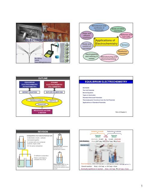
<strong>ELECTROCHEMISTRY</strong><br />
Mrs Billing<br />
GH840<br />
Caren.Billing@wits.ac.za<br />
Water and<br />
effluent<br />
treatment<br />
Study and<br />
control of<br />
corrosion<br />
Electroplating<br />
and refining of<br />
metals<br />
Manufacture and<br />
synthesis of<br />
chemicals<br />
Study of redox<br />
reactions<br />
Applications of<br />
Electrochemistry<br />
Manufacturing and<br />
electromachining<br />
Batteries and<br />
fuel cells<br />
Sensors<br />
Bioelectrochemistry<br />
EQUILIBRIUM<br />
<strong>ELECTROCHEMISTRY</strong><br />
(POTENTIOMETRY)<br />
NERNST EQUATION<br />
THERMODYNAMICS<br />
OUTLINE<br />
TRANSPORT<br />
DYNAMIC<br />
<strong>ELECTROCHEMISTRY</strong><br />
(VOLTAMMETRY)<br />
BUTLER-VOLMER EQN<br />
KINETICS<br />
EQUILIBRIUM <strong>ELECTROCHEMISTRY</strong><br />
REVISION<br />
The Cell Potential<br />
Nernst Equation<br />
Types of electrodes<br />
Standard Electrode Potentials<br />
Thermodynamic Functions from the Cell Potential<br />
Applications of Standard Potentials<br />
MOLECULES and IONS<br />
in MOTION<br />
Part of Chapter 6<br />
REVISION<br />
Oxidation at anode<br />
Reduction at cathode<br />
Composition of an electrochemical cell:<br />
2 electrodes: anode + cathode<br />
Connected together<br />
In contact with ionic conductor<br />
(solution, liquid, solid)<br />
Of the same composition<br />
V<br />
Galvanic cell: produces<br />
electricity due to<br />
spontaneous reaction.<br />
Cell Notation:<br />
Daniell Cell:<br />
electrode<br />
Separate<br />
phases<br />
in soln<br />
Salt<br />
bridge<br />
in soln<br />
Separate<br />
phases<br />
electrode<br />
Zn(s) | Zn 2+ (aq,1 M) | | Cu 2+ (aq,1 M) | Cu(s)<br />
Or different composition<br />
Need a salt bridge to<br />
complete the circuit<br />
Electrolytic cell: the nonspontaneous<br />
reaction is<br />
driven by an external current<br />
source.<br />
Zn(s) looses e − ’s<br />
Cu 2+ (aq) gains e − ’s<br />
Overall reaction: Zn(s) + Cu 2+ (aq) → Zn 2+ (aq) + Cu(s)<br />
Eventually equilibrium in reached: Zn(s) + Cu 2+ (aq) Zn 2+ (aq) + Cu(s)<br />
1
w max = ∆G<br />
Before Equilibrium<br />
The Cell Potential<br />
Consider a galvanic cell reaction:<br />
The cell can do electrical work by driving<br />
e − ’s through the external circuit.<br />
The larger the potential difference between the<br />
two electrodes, the more work can be done by<br />
each e−.<br />
Measure E cell by applying an opposing<br />
potential s.t. the reaction occurs reversibly<br />
and the composition is constant (no nett<br />
current flows).<br />
∆G = −nFE cell<br />
for electrical work for a<br />
reversible reaction<br />
At Equilibrium<br />
No more work can be done<br />
E cell = 0 V<br />
The composition in electrode compartment is expressed by:<br />
the reaction quotient, Q<br />
the equilibrium constant, K<br />
Derive Nernst equation:<br />
RT<br />
E = E<br />
o − ln Q<br />
nF<br />
Applies to:<br />
∆G = −nFE<br />
Half-reactions<br />
RT<br />
E<br />
nF<br />
and<br />
Cells<br />
RT<br />
nF<br />
o<br />
o<br />
= Ered<br />
− lnQred<br />
E = Ecell<br />
− lnQrxn<br />
Half-cell reaction written as a<br />
reduction reaction.<br />
Nernst Equation<br />
o<br />
∆G<br />
= ∆G<br />
+ RT ln Q<br />
2.303 RT<br />
E = E<br />
o − log Q<br />
nF<br />
E<br />
o<br />
cell<br />
= E<br />
o<br />
cathode<br />
− E<br />
o<br />
anode<br />
NOTE: E o used in the calculations are always for the reduction reactions.<br />
loge<br />
x<br />
log x =<br />
10<br />
loge<br />
10<br />
2 .303 log x = ln x<br />
0.05916<br />
E = E<br />
o − log Q at 25°C<br />
n<br />
E o = standard cell potential all reactants and products in their standard states,<br />
thus all activities = 1<br />
∆G = −nFE<br />
Do Self-test 6.7<br />
Standard Reduction Potentials in H 2 O at 25 o C<br />
The cell reaction is spontaneous<br />
if E cell > 0<br />
At equilibrium:<br />
∆G = 0 E cell = 0 and Q = K<br />
Strong oxidising<br />
agent<br />
Gibbs free energy, G<br />
∆G < 0<br />
E > 0<br />
∆G = 0<br />
E = 0<br />
∆G > 0<br />
E < 0<br />
RT<br />
E = E<br />
− lnQ<br />
nF<br />
RT<br />
0 E − lnK<br />
nF<br />
= nF <br />
ln K = E<br />
RT<br />
E > 0 <br />
spontaneous<br />
reduction<br />
reactants<br />
Extent of reaction<br />
products<br />
The steeper the slope, the greater<br />
the driving power of the cell.<br />
Recall:<br />
∆G°= –RT ln K<br />
∆G°= –nFE°<br />
E < 0 nonspontaneous<br />
reduction<br />
Strong reducing<br />
agent<br />
Example 1<br />
Consider the Daniell cell:<br />
Using the standard reduction potentials, calculate the equilibrium constant at 25 °C.<br />
Standard reduction potentials at 25 °C:<br />
Cu 2+ + 2e - → Cu(s)<br />
Zn 2+ + 2e - → Zn(s)<br />
Zn(s)<br />
ZnSO 4 (aq) CuSO 4 (aq) Cu(s)<br />
E o = +0.34 V<br />
E o = −0.76 V<br />
Do Self-test 6.8<br />
Metal/metal ion:<br />
e.g. Zn(s) in zinc ion solution<br />
M(s) | M n+ (aq)<br />
Metal-insoluble salt: M(s) | MX(s) | X - (aq)<br />
e.g. silver-silver chloride electrode<br />
−<br />
Ag(s)<br />
AgCl(s) Cl (aCl)<br />
AgCl(s) + e - Ag(s) + Cl - (aq)<br />
Inert electrode: Pt(s) | M n+ (aq), M p+ (aq)<br />
e.g. Pt immersed in a solution containing a redox couple<br />
4 + 3+<br />
Pt(s) Ce (aq),Ce (aq)<br />
Ce 4+ + e - Ce 3+<br />
o RT a<br />
E = E − ln<br />
F a<br />
Gas electrode:<br />
Zn 2+ + 2e - Zn(s)<br />
Pt(s) | X 2 (g) | X +/− (aq)<br />
e.g. a standard hydrogen electrode<br />
+<br />
Pt(s)<br />
H2(g)<br />
H (aq)<br />
2H + + 2e - H 2 (g)<br />
Types of Electrodes<br />
E<br />
E<br />
RT<br />
2F<br />
o<br />
= E − ln<br />
2+<br />
RT<br />
F<br />
o<br />
= E − ln a<br />
−<br />
Cl<br />
RT<br />
2F<br />
1<br />
a<br />
p<br />
3+<br />
Ce<br />
4+<br />
Ce<br />
o<br />
H2<br />
E = E − ln<br />
2<br />
a<br />
Zn<br />
+<br />
H<br />
2
Standard Electrode Potentials<br />
The potential of a half-cell is measured relative to the standard<br />
hydrogen electrode (SHE) under standard conditions.<br />
Pt(s) | H 2 (g) | H + (aq)<br />
activities = 1 mol kg -1<br />
E o SHE = 0 V at all temperatures fugacities = 1 atm<br />
Determining the standard potential of a silver-silver chloride electrode using<br />
a Harned cell:<br />
Pt⏐H 2 (g)⏐HCl(aq), a H+ , a Cl- ⏐AgCl(s)⏐Ag(s)<br />
Half-reactions:<br />
H + + e − → ½H 2 (g)<br />
anode E o<br />
1e - SHE = 0 V<br />
AgCl(s) + e − → Ag(s) + Cl − (aq) cathode<br />
Recall: E o is an intensive property!<br />
E o cell = Eo indicator – Eo reference<br />
SHE<br />
Overall reaction:<br />
AgCl(s) + ½H 2 (g) → H + (aq) + Ag(s) + Cl − (aq)<br />
Nernst equation:<br />
o RT a<br />
+<br />
a<br />
−<br />
H Cl<br />
E = E − ln<br />
cell cell<br />
F PH 2<br />
For SHE: P H2 = 1 atm<br />
o RT<br />
Ecell<br />
= Ecell<br />
− ln a + a −<br />
F H Cl<br />
Let a H+ = γ m ± H+ and a Cl- = γ ± m o RT 2 2<br />
Cl- Ecell = Ecell<br />
− ln (mHCl<br />
γ ± )<br />
F<br />
γ ± = mean activity coefficient<br />
m = molality (concentration in mol kg -1 )<br />
o RT 2 2<br />
Ecell = Ecell<br />
− ln (mHCl<br />
γ ± )<br />
F<br />
o RT 2 RT<br />
Ecell = Ecell<br />
− ln (mHCl<br />
) − ln ( γ ±<br />
F<br />
F<br />
2RT<br />
o 2RT<br />
Ecell<br />
+ ln mHCl<br />
= Ecell<br />
− ln γ ±<br />
F<br />
F<br />
Debye-Hückel law: log γ<br />
for a 1:1 electrolyte:<br />
±<br />
= −<br />
log γ ±<br />
2 .303 log x = ln x<br />
2<br />
)<br />
A z z<br />
= −<br />
+<br />
−<br />
ln = −A′<br />
γ ±<br />
I<br />
A I = −A<br />
mHCl<br />
If E o cell is known, then using E cell<br />
the activity coefficient γ ± can be<br />
calculated for a solution of<br />
molality m.<br />
m HCl<br />
1<br />
2<br />
I = m i z i<br />
2 i<br />
I<br />
1<br />
2<br />
[(m<br />
)( + 1) + (m<br />
H +<br />
2<br />
)( −1)<br />
]<br />
=<br />
2<br />
− Cl<br />
1<br />
I = [ 2(m )]<br />
HCl<br />
2<br />
Evaluating a standard potential from two others:<br />
E o +<br />
Cu 2 + =<br />
/ Cu(s)<br />
E o + = +<br />
Cu / Cu(s)<br />
0.340 V<br />
0.522 V<br />
E o =<br />
Cu 2 + +<br />
/ Cu<br />
Cu 2+ (aq) + 2e - → Cu(s) E o = 0.340 V (A)<br />
Cu + (aq) + e - → Cu(s) E o = 0.522 V (B)<br />
(A) – (B): Cu 2+ (aq) + e - → Cu + (aq) E o (C) = <br />
NOTE:<br />
Thermodynamic Functions from the Cell Potential<br />
This is NOT a cell reaction!!<br />
→ the electrons do NOT cancel out<br />
<br />
Redox couple Cu 2+ /Cu +<br />
→ Reduction reaction<br />
reduction<br />
oxidation<br />
2RT<br />
o 2RT<br />
E<br />
cell<br />
+ ln mHCl<br />
= Ecell<br />
+ A′<br />
m<br />
F<br />
F<br />
HCl<br />
y = c + m x<br />
Measure the cell potential for<br />
various HCl concentrations.<br />
Plot y vs x and extrapolate to the<br />
y-intercept to determine E o cell<br />
Applications of Standard Potentials<br />
1) The determination of activity coefficients<br />
2) The determination of equilibrium constants<br />
3) The electrochemical series<br />
4) The determination of thermodynamic functions<br />
Example 2<br />
The mean activity coefficients of HBr in 5.0 and 20.0 mmol kg –1 are 0.930 and 0.879,<br />
respectively. Consider a hydrogen electrode in HBr(aq) solution at 25 °C operating at<br />
1.15 atm.<br />
Calculate the change in the electrode potential when the molality of the acid solution<br />
is changed from 5.0 and 20.0 mmol kg –1 .<br />
Thermodynamics has the striking ability of to relate apparently unrelated<br />
relationships.<br />
<br />
∆G = −nFE<br />
E o cell used to calculate ∆Go f of ions in solution.<br />
Using the relationship<br />
<br />
dE ∆S<br />
=<br />
dT nF<br />
∂G<br />
<br />
= −S<br />
∂T<br />
p<br />
The temperature coefficient of E o cell gives the standard entropy<br />
of the cell reaction and hence entropies of ions in solution.<br />
Combining both relationships:<br />
<br />
<br />
<br />
dE<br />
∆H<br />
= ∆G<br />
+ T∆S<br />
= −nF<br />
E − T<br />
<br />
<br />
dT <br />
Non-calorimetric measurement of ∆H°<br />
and hence ∆H o f of ions in solution can<br />
be determined.<br />
3
Example 3<br />
Devise a cell in which the cell reaction is:<br />
Mn(s) + Cl 2 (g) → MnCl 2 (aq)<br />
Give the half reactions at the electrodes and from the standard cell potential of 2.54 V<br />
deduce the standard potential for the Mn 2+ /Mn(s) redox couple.<br />
Given: E°(Cl 2 /Cl - ) = +1.36 V<br />
Example 4<br />
Estimate the cell potential at 25°C for<br />
Ag(s)|AgBr(s)|KBr(aq, 0.050 mol kg –1 )||Cd(NO 3 ) 2 (aq,0.0034 mol kg –1 )|Cd(s)<br />
E°(R-H) = –0.40 V E°(L-H) = +0.07 V (assume non-ideal solutions)<br />
Write the spontaneous electrochemical reaction.<br />
Example 5<br />
The standard potential of the cell below at 25 °C is 0.95 V.<br />
Ag(s) |AgI(s) | AgI(aq) | Ag(s)<br />
Calculate: a) its solubility constant and b) the solubility of AgI .<br />
MOLECULAR MOTION IN LIQUIDS<br />
Mass Transport<br />
Migration of ions - Conductivities of Electrolyte Solutions<br />
Mobilities of Ions<br />
Diffusion of Ions<br />
Part of Chapter 20<br />
Mass Transport<br />
Three main ways to transport ions to the surface of an electrode<br />
→ called mass transport<br />
Conductivities of Electrolyte Solutions<br />
Ions can be dragged through the solvent by applying a potential difference<br />
between two electrodes in solution.<br />
MIGRATION<br />
To measure conductivity:<br />
Incorporate conductivity cell into<br />
one arm of resistance bridge and<br />
search for balance point.<br />
R 3<br />
Convection<br />
Movement due to<br />
mechanical intervention.<br />
e.g. stirring, pumping,<br />
shaking<br />
Affects molecules and<br />
ions in solution.<br />
Diffusion<br />
Movement due to<br />
concentration gradient.<br />
e.g. movement across a<br />
cell membrane<br />
Affects molecules and<br />
ions in solution.<br />
Migration<br />
Movement due to applied<br />
electric field.<br />
e.g. in an electrolysis cell<br />
Affects only ions in<br />
solution.<br />
1 <br />
R =<br />
κ A<br />
1 <br />
κ =<br />
R A<br />
C<br />
κ =<br />
R<br />
R = resistance of solution (Ω)<br />
κ = conductivity (S cm -1 )<br />
= distance between electrodes<br />
A = area of electrodes<br />
C = cell constant<br />
κ depends on the number of ions in a solution.<br />
R 4<br />
2<br />
R 1<br />
R R =<br />
1 2<br />
R R<br />
3<br />
R 4<br />
Resistance bridge R 1R<br />
= R R3<br />
4 2<br />
Note: use ac current (ν~1kHz)<br />
to avoid electrolysis and<br />
polarisation of the electrodes<br />
which would change the<br />
composition of the solution at<br />
the electrode surfaces.<br />
4
Measuring the conductivity of tap water:<br />
κ<br />
=<br />
c<br />
Λ<br />
Λ<br />
m = molar conductivity (S cm 2 mol -1 )<br />
m c = molarity<br />
If κ ∝ c, the molar conductivity should be<br />
independent of the concentration of an<br />
electrolyte. Is this the case<br />
Parallel<br />
plates<br />
293.3 µS / cm<br />
1 S = 1 Siemen<br />
= 1 Ω -1<br />
NO!<br />
Molar conductivity varies with<br />
concentration because:<br />
- no. of ions in solution may not be<br />
proportional to concentration (especially<br />
for weak electrolytes)<br />
- ions interact strongly with one another<br />
reducing effective charge<br />
NB: Don’t confuse conductivity (κ) with conductance (G)<br />
Strong electrolyte – Λ m<br />
decreases slightly as<br />
conc increases.<br />
Weak electrolyte –<br />
normal Λ m at low conc,<br />
but Λ m decreases sharply<br />
as conc increases.<br />
1<br />
G =<br />
R<br />
Kohlrausch’s law:<br />
At low concentrations, molar conductivities vary with the square root of conc.<br />
Λ = Λ − K c<br />
m<br />
Λ o m<br />
= ν<br />
o<br />
m<br />
+<br />
λ<br />
+<br />
+ ν<br />
−λ<br />
−<br />
STRONG ELECTROLYTES<br />
Λ m o = limiting molar conductivity<br />
(ions are infinitely far apart no interaction)<br />
K → related to stoichiometry of electrolyte<br />
Kohlrausch’s law of independent migration of ions:<br />
Λ m o → expressed as sum of contributions from its individual ions.<br />
λ = limiting molar conductivity of ions<br />
ν = no. of ions per formula unit of electrolyte<br />
H +<br />
34.96 OH -<br />
19.91<br />
Na + 5.01 Cl -<br />
7.63<br />
K + 7.35 Br -<br />
7.81<br />
Zn 2+ 10.56 SO 2-<br />
4 16.00<br />
e.g. for MgCl 2 : ν + = 1 ν − = 2<br />
Limiting ionic conductivies in water at 298 K, λ /mS m 2 mol -1<br />
Weak electrolytes do NOT dissociate completely,<br />
conductivity of weak electrolytes depends on the degree of ionization (α)<br />
e.g. HA + H 2 O A - + H 3 O +<br />
+ −<br />
[H3O<br />
][A ]<br />
+<br />
K<br />
[ H3O<br />
] = αc<br />
a =<br />
[HA]<br />
−<br />
[ A ] = αc<br />
2<br />
α c<br />
Ka<br />
=<br />
[ HA] = ( 1−<br />
α)c<br />
1 − α<br />
At infinite dilution the electrolyte is fully<br />
ionised :<br />
Λ o m<br />
= ν<br />
+<br />
λ<br />
+<br />
+ ν<br />
−λ<br />
−<br />
At very low conc’s:<br />
Ostwald’s<br />
dilution<br />
law<br />
WEAK ELECTROLYTES<br />
Λ = α<br />
o<br />
m<br />
Λ m<br />
1 1 Λ<br />
mc<br />
= +<br />
o<br />
Λ<br />
m Λ<br />
m K<br />
( Λ ) o 2<br />
1 1 1<br />
= + Λ<br />
mc<br />
o<br />
o 2<br />
Λ<br />
m Λ<br />
m K<br />
a<br />
( Λ<br />
m<br />
)<br />
y c m x<br />
a<br />
m<br />
(c = formal conc of HA)<br />
Example 6<br />
Calculate the degree of ionization and the acid dissociation constant at 298 K for a<br />
0.010 M acetic acid solution that has a resistance of 2220 Ω. The resistance of a 0.100<br />
M potassium chloride solution was also found to be 28.44 Ω.<br />
Λ m (0.1 M KCl) = 129 S cm 2 mol -1<br />
λ o (H + ) = 349.6 S cm 2 mol -1<br />
λ o (CH 3 COO - ) = 40.9 S cm 2 mol -1<br />
Example 7<br />
The molar conductivity of a strong electrolyte in water at 25 °C was found to be 109.9<br />
S cm 2 mol -1 for a concentration of 6.2 × 10 -3 mol L -1 and 106.1 S cm 2 mol -1 for a<br />
concentration of 1.5 × 10 -3 mol L -1 .<br />
Estimate the limiting molar conductivity of the electrolyte.<br />
5
Example 8<br />
The limiting molar conductivities of KCl, KNO 3 , and AgNO 3 are 149,9, 145.0, and 133.4<br />
S cm 2 mol -1 , respectively (all at 25 °C).<br />
What is the limiting molar conductivity of AgCl at this temperature<br />
To understand conductivity measurements, we need to understand why<br />
ions move at different rates<br />
Motion of ions is largely random, but in the presence of an electric field the<br />
motion is biased → migration<br />
DC, uniform electric<br />
field is applied<br />
Mobilities of Ions<br />
Electric field:<br />
∆φ<br />
ε =<br />
<br />
∆φ = potential difference<br />
= distance between electrodes<br />
ε = electric field<br />
V source<br />
+ ∆φ<br />
+<br />
-<br />
<br />
Force acting on the ion due to electric field:<br />
ze∆φ<br />
ze = charge of ion<br />
F e<br />
= zeε<br />
=<br />
<br />
e = 1.602×10 -19 C<br />
causes ion to accelerate towards oppositely<br />
charge electrode.<br />
But ion undergoes frictional retardation<br />
when moving through the solvent:<br />
F Fric<br />
viscosity drag<br />
= fs = 6<br />
πη<br />
as<br />
s = speed of ion<br />
η = viscosity of solvent<br />
a = radius of ion<br />
The two forces (one due to the electric field force and the other due to the viscosity<br />
drag, interactions between ions, etc.) act in the opposite directions.<br />
Eventually, these forces are balanced<br />
F e = F Fric<br />
and the ions reach a terminal speed called the drift speed.<br />
zeε<br />
= 6<br />
πη<br />
as<br />
Self-study:<br />
What is the Grotthaus mechanism which is used to explain the very high mobility of<br />
H + in water<br />
zeε<br />
Drift speed: s =<br />
6πη<br />
a<br />
stronger electric field ε<br />
faster ions drift<br />
s = uε<br />
u = ionic mobility =<br />
ze<br />
6<br />
πη<br />
a<br />
The drift speed<br />
governs the rate<br />
at which charge<br />
is transported.<br />
theoretical<br />
measurable<br />
LINK between mobility and molar conductivity<br />
∴ expect the conductivity to decrease with increasing solution viscosity and<br />
increasing ion size.<br />
Ionic mobilities in water at 298 K,<br />
u /10 -8 m 2 s -1 V -1<br />
H + 36.23 OH - 20.64<br />
Na + 5.19 Cl - 7.91<br />
K + 7.62 Br - 8.09<br />
Zn 2+ 5.47 SO 2-<br />
4 8.29<br />
However, we see the larger ion (with the<br />
same charge) has a larger mobility.<br />
Need to consider:<br />
a = hydrodynamic radius<br />
i.e. includes hydration sphere<br />
Small ions are more extensively<br />
hydrated that larger ions (due to the<br />
stronger electric field)<br />
For cations and anions:<br />
λ = zuF<br />
And for very diluted solutions:<br />
o<br />
Λ m = ( ν+ z+<br />
u+<br />
+ ν−z−u<br />
− )F<br />
Faraday’s constant = F = N A e<br />
Since Λ o m = ν+ λ+<br />
+ν−λ−<br />
Ion-ion interactions affecting mobilities:<br />
In ionic solutions the ion-atmosphere also needs to be<br />
considered when ions migrate.<br />
When an electric field is introduced, two effects occur:<br />
Relaxation effect:<br />
When an electric field is introduced the ionic atmosphere is<br />
distorted as it drags behind moving charge.<br />
Central ion and atmosphere opposite in charge retardation<br />
of moving ion.<br />
Electrophoretic Effect:<br />
The ion-atmosphere moves in the opposite direction to the<br />
central ion which lead to the reduction in ion mobility.<br />
Both effects results in lower mobilities!<br />
Fick’s first law of diffusion:<br />
The flux (J) of particles is proportional to the concentration gradient.<br />
dc<br />
J = −D<br />
dx<br />
D = diffusion coefficient<br />
c = molar concentration<br />
x = distance<br />
Einstein equation:<br />
Stokes-Einstein equation:<br />
Nernst-Einstein equation:<br />
Applies to ions and uncharged particles in a solution.<br />
RT<br />
D = u<br />
zF<br />
Diffusion of Ions<br />
kT<br />
D =<br />
6<br />
πη<br />
a<br />
c 1 > c 2<br />
c 1<br />
c 2<br />
J<br />
substitute expression for u<br />
k = Boltzmann constant = 1.381×10 -23 J K -1<br />
Λ =<br />
F 2<br />
o 2<br />
( ν+ z+<br />
D+<br />
+ ν−z<br />
2 Or for a<br />
m −D−<br />
)<br />
λ+ =<br />
F 2<br />
o<br />
( ν + z<br />
2<br />
+ D+<br />
)<br />
RT<br />
single ion: RT<br />
c<br />
Do Self-test 20.4<br />
dc<br />
dx<br />
x<br />
6
Fick’s second law of diffusion or the<br />
diffusion equation:<br />
2<br />
∂c<br />
∂ c<br />
= D<br />
2<br />
∂t<br />
∂x<br />
→ describes time<br />
dependence of the<br />
diffusion process<br />
Diffusion coefficients at 298 K, 10 -9 m 2 s -1 Example 9<br />
H + in water<br />
9.31<br />
The mobility of the NO 3- ion in aqueous solution at 25 °C is 7.40×10 -8 m 2 s -1 V -1 .<br />
Na + in water<br />
1.33<br />
(Viscosity of water is 0.89110 -3 kg m -1 s -1 ).<br />
sucrose in water 0.522<br />
Calculate its diffusion coefficient and the effective radius at this temperature.<br />
It shows that the rate of change of conc is proportional to the<br />
curvature (the second derivative) of the concentration with<br />
respect to the distance.<br />
This equation shows that:<br />
1) If the concentration changes sharply from point to<br />
point, then the concentration changes rapidly in time.<br />
c<br />
vs<br />
c<br />
x<br />
x<br />
2) If the curvature = 0, then the concentration does not<br />
change in time.<br />
3) If the concentration decreases linearly with distance,<br />
then the concentration is constant at any point,<br />
because the inflow is exactly balanced by the outflow<br />
of particles or ions.<br />
c<br />
x<br />
Remember: in the calculations you have to show the work on units.<br />
Without that, the work might be considered as not done at all.<br />
DYNAMIC <strong>ELECTROCHEMISTRY</strong><br />
Double Layer at the Electrode-Solution Interface<br />
Dynamic Equilibrium<br />
Butler-Volmer Equation<br />
No Mass Transport Effects<br />
Mass Transport Effects<br />
Tafel Plot<br />
Electrolysis and Galvanic Cells<br />
Double Layer at the Electrode-Solution Interface<br />
Electrode reaction = heterogeneous chemical process<br />
e - ’s move from electrode surface to chemical species in solution (at the surface), or<br />
vice versa<br />
Diffusion layer – region<br />
dominated by unequal<br />
(1 µm − 1 mm) charge distribution<br />
Region of charge neutrality<br />
Part of Chapter 22<br />
(1 − 10 nm)<br />
Double layer generated due<br />
to electrostatic forces<br />
Faradaic process:<br />
Helmholtz Model<br />
Gouy-Chapman Model<br />
Electrons transferred across the electrode-solution interface (reduction/oxidation)<br />
Governed by Faraday’s Law: current ∝ charge<br />
Non-Faradaic process:<br />
Under some conditions an electrodesolution<br />
interface shows a range of<br />
potentials where no charge transfer<br />
reaction occurs.<br />
E.g. capacitive or charging currents<br />
i<br />
Charging currents decay rapidly<br />
after applying a potential.<br />
t<br />
φ M<br />
+<br />
+<br />
+<br />
+<br />
+<br />
+<br />
+<br />
Electrode<br />
-<br />
-<br />
-<br />
-<br />
-<br />
-<br />
-<br />
Solution<br />
φ s<br />
Distance<br />
Double layer is like a capacitor<br />
20-40 µF/cm 2<br />
∆φ = φ M - φ S = Galvani potential difference<br />
The potential difference between points<br />
in the bulk metal and the bulk solution.<br />
φ M<br />
Electrode<br />
OHP<br />
Solvated<br />
ions<br />
φ S<br />
φ M<br />
+<br />
+<br />
+<br />
+<br />
+<br />
+<br />
+<br />
Electrode<br />
Solution<br />
Distance<br />
Double layer has no thickness and is<br />
diffused by thermal motion of ions<br />
Stern Model<br />
φ M<br />
+<br />
+<br />
+<br />
+<br />
+<br />
+<br />
+<br />
Electrode<br />
-<br />
-<br />
-<br />
-<br />
-<br />
-<br />
-<br />
OHP<br />
rigid Helmholz plane<br />
Diffusion of<br />
charges caused<br />
by thermal<br />
motion of ions<br />
Distance<br />
7
Exchange Current Density<br />
Under zero current conditions:<br />
Dynamic Equilibrium<br />
Ox + ne - Red<br />
o RT a<br />
Eeq<br />
= E − ln<br />
nF a<br />
Re d<br />
Ox<br />
EQUILIBRIUM!<br />
Overpotential (η):<br />
the difference between the applied potential and the<br />
equilibrium potential.<br />
η = E – E eq<br />
Equilibrium potential: potential where i = 0<br />
By definition, no net chemical change occurs i = 0<br />
However, this is a dynamic equilibrium! i = ia + ic<br />
= 0<br />
Increasing rate of reduction<br />
η = E – E eq<br />
E eq<br />
Increasing rate of oxidation<br />
η = E – E eq<br />
i.e. there is still current flowing:<br />
i a = −ic<br />
= io<br />
E eq<br />
exchange current<br />
η > 0<br />
Recall: current is the variation of charge with time:<br />
current ∝ rate of electron transfer<br />
dq<br />
i =<br />
dt<br />
η < 0<br />
i o is a measure of the electron transfer activity in both cathodic and anodic directions<br />
at equilibrium.<br />
It is a very useful kinetic parameter in dynamic electrochemistry.<br />
Rate of e - transfer depends on the electrode potential which drives the<br />
transfer of e - ’s.<br />
Current is defined as:<br />
i = nFAν<br />
A = surface area of electrode<br />
ν = reaction rate<br />
Forward reaction:<br />
Reverse reaction:<br />
k k ox<br />
Ox + ne - red<br />
Red<br />
Red Ox + ne-<br />
ν<br />
red<br />
= k<br />
red<br />
C<br />
i<br />
ν c<br />
red<br />
=<br />
nFA<br />
Butler-Volmer<br />
Equation<br />
ox<br />
1 st order<br />
Current at electrode:<br />
ν = k C<br />
ox<br />
ox<br />
i<br />
ν a<br />
ox<br />
=<br />
nFA<br />
Overall rate:<br />
1<br />
ν = νox<br />
− νred<br />
= koxCred<br />
− kredCox<br />
= (ia<br />
− ic<br />
)<br />
nFA<br />
i = ia<br />
− ic<br />
= nFA(k oxCred<br />
− kredCox<br />
)<br />
red<br />
Note: c red or c ox refers to the<br />
conc’s near the electrode surface<br />
Forward reaction:<br />
Reverse reaction:<br />
k<br />
Ox + ne - red<br />
k ox<br />
Red<br />
Red Ox + ne-<br />
Current at electrode:<br />
The rate constant varies with applied potential (in an exponential way):<br />
(1−α<br />
)nF<br />
−αnF<br />
η<br />
η<br />
o<br />
o<br />
RT<br />
RT<br />
k = kred<br />
= k e<br />
ox<br />
k e<br />
k o = standard rate constant (k when potential applied is E eq )<br />
α = transfer coefficient (0 < α < 1) → symmetry factor<br />
(1− α)nF<br />
o<br />
i = nFAk C RT<br />
<br />
rede<br />
<br />
i = ia<br />
− ic<br />
= nFA(k oxCred<br />
− kredCox<br />
)<br />
η<br />
− Coxe<br />
− αnF<br />
η <br />
RT<br />
<br />
<br />
(1− α)nF<br />
− αnF<br />
η<br />
η <br />
i = i RT − RT<br />
o e e<br />
<br />
<br />
<br />
<br />
Butler-Volmer equation<br />
and<br />
o<br />
io = nFAk C<br />
Current (rate of reaction) depends on:<br />
• Electrode area, A<br />
• Concentration of reactant, C<br />
• Temperature<br />
• The kinetic parameters i o and α<br />
• Overpotential, η<br />
Current density, j:<br />
i<br />
j =<br />
A<br />
(1− α)nF<br />
− αnF<br />
η<br />
η <br />
j = j RT − RT<br />
o e e<br />
<br />
<br />
<br />
<br />
(1−α)nF<br />
− αnF<br />
η<br />
η <br />
i = i RT − RT<br />
o e e<br />
<br />
<br />
<br />
<br />
i = nFAν<br />
j is independent of electrode area<br />
Butler-Volmer equation in<br />
terms of current density<br />
For small overpotentials (η < ~10 mV):<br />
nF<br />
j = joη<br />
RT<br />
In most practical situations, only the forward or the reverse reaction is significant and<br />
a simplified equation is sufficient.<br />
Large, positive overpotential predominantly oxidation:<br />
In practise, η ≥ ~ +0.12/n V<br />
j<br />
(1−α<br />
)nF<br />
η<br />
RT<br />
= j e o<br />
(1− α)nF<br />
ln j = ln jo<br />
+ η<br />
RT<br />
Large, negative overpotential predominantly reduction:<br />
In practise, η ≤ ~ -0.12/n V<br />
j<br />
−αnF<br />
η<br />
RT<br />
= j e o<br />
αnF<br />
ln j = ln jo<br />
− η<br />
RT<br />
(1− α)nF<br />
j = j RT<br />
o e<br />
<br />
<br />
η<br />
− e<br />
Anodic current<br />
− αnF<br />
η <br />
RT<br />
<br />
<br />
Cathodic current<br />
i.e. η nF < 1<br />
RT<br />
Low field region<br />
High field region<br />
Tafel equations<br />
8
(1− α)nF<br />
ln j = ln jo<br />
+ η<br />
RT<br />
Tafel Plot<br />
Tafel Plot<br />
Anodic current<br />
Butler-Volmer: No Mass Transport Effects<br />
j<br />
j a<br />
High field<br />
Oxidation: Red → Ox + ne -<br />
For oxidation reaction<br />
anodic current:<br />
nF<br />
slope = (1−<br />
α)<br />
RT<br />
∴ find α<br />
j = j a + j c<br />
Low field<br />
i ∝ E<br />
E<br />
ln j o<br />
Deviation from linearity at low<br />
η as the reverse reaction can<br />
no longer be ignored<br />
High field<br />
j c<br />
Reduction: Ox + ne - → Red<br />
<br />
j = jo<br />
e<br />
<br />
Anodic<br />
current<br />
(1−α<br />
)nF<br />
η<br />
RT<br />
− e<br />
Cathodic<br />
current<br />
−αnF<br />
RT<br />
η <br />
<br />
<br />
Focusing on low field region<br />
j<br />
Oxidation<br />
j a<br />
Effect of transfer coefficient (α) on j vs η relationship:<br />
j<br />
α = 0.25 α = 0.5<br />
η0<br />
Oxidation favoured<br />
α = 0.75<br />
j a = j o<br />
-j c = j o<br />
E = E eq potential at<br />
zero current flow<br />
E<br />
Reduction:<br />
Ox + ne - → Red<br />
Oxidation:<br />
Red → Ox + ne -<br />
η<br />
j c<br />
Reduction<br />
Reduction favoured<br />
(1− α)nF<br />
− αnF<br />
η<br />
η <br />
j = j RT − RT<br />
o e e<br />
<br />
<br />
<br />
<br />
α = the fraction of applied potential that<br />
influences the rate of electrochemical rxn<br />
Butler-Volmer: Mass Transport Effects<br />
Assumption in derivation of Butler-Volmer equation:<br />
negligible conversion of electroactive species at low current densities<br />
uniformity of concentration near the electrode<br />
j<br />
Predicted by the<br />
Butler-Volmer equation<br />
The Butler-Volmer equation fails at high current densities → current is limited<br />
by transport of ions towards the electrode.<br />
Larger η is needed to produce given current.<br />
η<br />
Current<br />
controlled only<br />
by mass<br />
transport<br />
This effect is called concentration polarisation<br />
and its contribution to the total overpotential is called the polarisation<br />
overpotential, η c .<br />
Current<br />
controlled only<br />
by electron<br />
transfer and j 0<br />
Exponential<br />
increase in<br />
current with η<br />
(B-V equation)<br />
Current<br />
controlled by η<br />
and transport<br />
9
Example 10<br />
The electron transfer coefficient of a certain electrode in contact with the redox couple<br />
M 3+ / M 4+ in aqueous solution at 25 °C is 0.39. The current density is found to be 55.0<br />
mA cm –2 when the overvoltage is 125 mV.<br />
What is the overvoltage required for a current density 75.0 mA cm –2 <br />
What is the exchange current density<br />
Example 11<br />
The exchange current density and the electron transfer coefficient for the reaction<br />
2H + + 2e H 2 (g) on nickel at 25 °C are 6.3 × 10 –6 A cm –2 and 0.58, respectively.<br />
Determine what current density would be required to obtain an overpotential of 0.20 V<br />
as calculated from the Butler-Volmer equation and the Tafel equation.<br />
Electrolysis Cells:<br />
Electrolysis and Galvanic Cells<br />
To induce current to flow through an electrolytic cell, have to apply a<br />
potential difference greater than that required to reach equilibrium:<br />
E applied > E eq<br />
In theory:<br />
Have to also overcome the cell overpotential:<br />
η cell = |η c | + |η a | + | iR s |<br />
There is an activation or charge<br />
transfer overpotential (η a and η c )<br />
at the anode and cathode.<br />
E eq = -E cell<br />
Additionally, the rate of e - transfer depends on the<br />
electrode potential which drives the transfer of e - ’s.<br />
E applied > E eq + |η cell |<br />
∆G > 0<br />
Ohmic drop due to the solution E cell < 0<br />
resistance, ∴ apply an overpotential to<br />
drive current through the solution. V = IR<br />
j<br />
η<br />
Many other factors also need to be taken into account<br />
E.g.: The magnitude of the exchange current density (j o ) also determines the<br />
overpotential required for a significant current to flow:<br />
j<br />
Decreasing j o<br />
For high j o :<br />
observable current at low η<br />
η<br />
Galvanic Cells:<br />
Conversely, in a galvanic cell a smaller potential difference is<br />
generated than expected due to these overpotentials.<br />
V<br />
j o /A m -2 : 10 10 2 10 3<br />
Self-test 6.7<br />
Express the formation of H 2 O from H 2 and O 2 in acidic solution (a redox reaction)<br />
as the difference of two reduction reactions.<br />
(You may need to consult the full table of standard reduction potentials in the Appendix)<br />
Self-test 6.8<br />
Write the half-reaction and the reaction quotient for a chlorine gas electrode.<br />
Self-test 20.4<br />
Use the experimental value of the mobility to evaluate the diffusion coefficient, the<br />
limiting molar conductivity and the hydrodynamic radius of the NH 4+ ion in<br />
aqueous solution. (u = 7.63 × 10 -8 m 2 s -1 V -1 )<br />
10