Chapter 11: Sprinkle Irrigation - NRCS Irrigation ToolBox Home Page

United States
Department of
Agriculture
Soil
Conservation
Service
National
Engineering
Handbook
Section 15
Irrigation
Chapter 11
Sprinkle
Irrigation

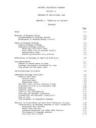
Contents
@ Adaptability .......................................................................... 11-1
Advantages ........................................................................ 11-2
Disadvantages ...................................................................... 11-2
@ Types of systems ..................................................................... 11-3
Periodic-move ....................................................................... 11-3
Hand-movelateral ................................................................. 11-3
End-towlateral .................................................................... 11-4
Side-rolllateral .................................................................... 11-4
Side-movelateral .................................................................. 11-5
Fixedsprinkler .....................................................................-11-5
Solid-setportable .................................................................. 11-5
Buriedlaterals .................................................................... 11-6
Gunandboomsprinklers ........................................................... 11-6
Continuous-movelateral .......................................... 11-7
Centerpivot ...................................................................... 11-7
Travelings~rinkler ................................................................. 11-8
Linear-movelateral ................................................................ 11-9
Other sprinklesystems ............................................................... 11-9
Perforatedpipe .................................................................... 11-9
Hose-fedsprinklergrid ............................................................. 11-9
Orchardsprinkler .................................................................. 11-9
@ Planning concepts ..................................................................... 11-10
gn.. .................................................................. 11-10
Capacityrequirements ............................................................. i.11-11
Fixedsystems ..................................................................... 11-15
Continuous-movesystems ........................................................... 11-16
Depthofapphcation ................................................................. 11-16
Water-holding capacity ............................................................. 11-17
Root depth ....................................................................... 11-17
Applicationdepthandfrequency ..................................................... 11-17
Intake and optimum application rates .................................................. 11-18
Periodic-move and fixed systems ..................................................... 11-20
Continuous~movesystems ........................................................... 11-21
Sprinkle irrigation efficiency .......................................................... 11-21
Uniformity ....................................................................... 11-21
Waterloss ......................................................................... 11-23
Application ....................................................................... 11-24
@ Design procedure. ..................................................................... 11-25
7..
Periodic-moveandfixedsystems ....................................................... 11-25
Sprinkler selection ................................................................. 11-26
Systemlayout ..................................................................... 11-43
Lateraldesi gn ..................................................................... 11-49
Mainlinedesign ................................................................... 11-57
Pressure requirements ..............................................................11-73
Selection of pump and power unit .................................................... 11-79
Fieldtest data .................................................................... 11-79
Travelingsprinklesystem ............................................................ 11-84
Sprinkler and traveler selection ...................................................... 11-84
Systemlayout ..................................................................... 11-89
Center-pivotdesi gn .................................................................. 11-90
Systemcapacity ................................................................... 11-90
e
Preliminarydesi
Page

Application intensity ............................................................... 11-91
Sprinkler-nozzle configuration ........................................................ 11-93
Lateralhydraulics ................................................................. 11-95
Operatingpressures ................................................................ 11-99
Elevationdischarge relationship ...................................................... 11-99
Machineselection ..................................................................l 1-101
Field test data .................................................................... 11-101
..................................................................
Sprinkler-nozzle configuration ........................................................ 11 - 109
.........................................................
....................................................
......................................
Fertilizermaterials ................................................................. 11-111
Fertilizer applications .............................................................. 11-112
Applying soil amendments ..........................................................11- 112
Applying pesticides ................................................................ 11-112
.............................................................
Designconsiderations .............................................................. 11-113
Linear-move system 11-109
@ Special uses of sprinkle systems 11-110
Federal. state. and local regulations 11-110
Applying fertilizers. soil amendments, and pesticides 11-110
Disposing of wastewater -11-113
Hardware ................................A.............................. 1-114
Frost protection ..................................................................... 11-114
.............................................................
Frost control operation 11-115
Bloomdelay ..................................................................... 1-11
Microclimate control ................................................................. 11-11
@) Installation and operation of sprinkle systems ............................................. 11-117
@Appendix .........................................................v...... 1-118

Chapter 11
Sprinkle Irrigation
Adaptability
Sprinkle irrigation is the application of water in
the form of a spray formed from the flow of water
under pressure through small orifices or nozzles.
The pressure is usually obtained by pumping, although
it may be obtained by gravity if the water
source is high enough above the area irrigated.
Sprinkle irrigation systems can be divided into
two general categories. In periodic-move and fixed
systems the sprinklers remain at a fixed position
while irrigating, whereas in continuous-move systems
the sprinklers operate while moving in either a
circular or a straight path. The periodic-move systems
include hand-move and wheel-line laterals,
hose-fed sprinkler grid, perforated pipe, orchard
sprinklers, and gun sprinklers. The dominant continuous-move
systems are centerpivot and traveling
sprinklers.
With carefully designed periodic-move and fixed
systems, water can be applied uniformly at a rate
based on the intake rate of the soil, thereby preventing
runoff and consequent damage to land and
to crops. Continuous move systems can have even
higher uniformity of application than periodic-move
and fixed systems, and the travel speed can be adjusted
to apply light watering that reduces or elimi-
Sprinkle irrigation is suitable for most crops. It is
also adaptable to nearly all irrigable soils since
sprinklers are available in a wide range of discharge
capacities. For periodic-move systems with proper
spacing, water may be applied at any selected rate
above 0.15 inch per hour (iph). On extremely finetextured
soils with low intake rates, particular care
is required in the selection of proper nozzle size,
operating pressure, and sprinkler spacing to apply
water uniformly at low rates.
Periodic-move systems are well suited for irrigation
in areas where the crop-soil-climate situation
does not require irrigations more often than every 5
to 7 days. Light, frequent irrigations are required
on soils with low water holding capacities and shallow-rooted
crops. For such applications, fixed or
continuously moving systems are more adaptable;
however, where soil permeability is low, some of the
continuously moving systems, such as the centerpivot
and traveling gun, may cause runoff problems.
In addition to being adaptable to all irrigation
frequencies, fixed systems can also be designed and
operated for frost and freeze protection, blossom delay,
and crop cooling.
The flexibility of present-day sprinkle equipment,
and its efficient control of water application make
the method's usefulness on most topographic conditions
subject only to limitations imposed by land
use capability and economics.

Advantages
Some of the most important advantages of the
sprinkle method are:
1, Small, continuous streams of water can be
used effectively,
2. Runoff and erosion can be eliminated,
3. Problem soils with intermixed textures and
profiles can be properly irrigated.
4. Shallow soils that cannot be graded without
detrimental results can be irrigated without grading.
5. Steep and rolling topography can be easily irrigated.
6. Light, frequent waterings can be efficiently applied.
7. Crops germinated with sprinkler irrigation
may later be surface irrigated with deeper applications.
8. Labor is used for only a short period daily in
each field.
9. Mechanization and automation are practical to
reduce labor.
10. Fixed systems can eliminate field labor dur.
ing the irrigation season.
11. Unskilled labor can be used because decisions
are made by the manager rather than by the irriga
tor.
12. Weather extremes can be modified by increasing
humidity, cooling crops, and alleviating freezing
by use of special designs.
13. Plans for intermittent irrigation to supplement
erratic or deficient rahfall, or to start early
grain or pasture can be made with assurance of adequate
water.
14. Salts can be effectively leached from the soil.
15. High application efficiency can be achieved
by a properly designed and operated system.
Disadvantages
Important disadvantages of sprinkle irrigation
are:
1. High initial costs must be depreciated. For
simple systems these costs, based on 1980 prices,
range from $75 to $150 per acre; for mechanized
and self-propelled systems, from $200 to $300; and
for semi and fully automated fixed systems from
$500 to $1,000.
2. Cost of pressure development, unless water is
delivered to the farm under adequate pressure, is
about $0.20 per acre-ft, of water for each pound per
square inch (psi) of pressure, based on $0.751gal for
diesel or $O.OGIKWH for electricity.
3. Large flows intermittently delivered are not
economical without a reservoir, and even a minor
fluctuation in rate causes difficulties.
4, Sprinklers are not well adapted to soils having
an intake rate of less than 0.15 inches per hour
(iph).
5. Windy and excessively dry locations appreciably
lower sprinkler irrigation efficiency.
6. Field shapes, other than rectangular, are not
convenient to irrigate especially with mechanized
sprinkle systems.
7. Cultural operations must be meshed with the
irrigation cycle.
8. Surface irrigation methods an suitable soils
and slopes have higher potential irrigation efficiency.
9. Water supply must be capable of being cut off
at odd hours when the soil moisture deficiency is
satisfied.
10. Careful managemmt must be exercised to obtain
the high potential efficiency of the method.
11. Systems must be designed by a competent
specialist with full consideration for efficient irrigation,
economics of pipe sizes and operation, and convenience
of labor.
12. When used in overhead sprinklers, irrigation
water that has high concentrations of bicarbonates
may affect the quality of fruit.
13. Saline water may cause problems because salt
may be absorbed by the leaves of some crops.
Sprinkle irrigation can be adapted to most climatic
conditions where irrigated agriculture is
feasible. Extremely high temperatures and wind
velocities, however, present problems in some areas,
especially where irrigation water contains large
amounts of dissolved salts.
Crops such as grapes, citrus, and most tree crops
are sensitive to relatively low concentrations of
sodium and chloride and, under low humidity conditions,
may absorb toxic amounts of these salts from
sprinkle-applied water falling on the leaves. Because
water evaporates between rotations of the
sprinklers, salts concentrate more during this alternate
wetting and drying cycle than if sprayed continuously.
Plants may be damaged when these salts
are absorbed. Toxicity shows as a leaf burn (necrosis)
on the outer leaf-edge and can be confirmed
by leaf analysis. Such injury sometimes occurs
when the sodium concentration in the irrigation wa-

Types of Systems
ter exceeds 70 pprn or the chloride concentration exceeds
105 ppm. Irrigating during periods of high
humidity, as at night, often greatly reduces or
eliminates this problem.
Annual and forage crops, for the most part, are
not sensitive to low levels of sodium and chloride.
Recent research indicates, however, that they may
be more sensitive to salts taken up through the leaf
during sprinkling than to similar water salinities
applied by surface or trickle methods. Under extremely
high evaporative conditions, some damage
has been reported for more tolerant crops such as
alfalfa when sprinkled with water having an electrical
conductivity (EG) = 1.3 mmhoslcm and containing
140 pprn sodium and 245 pprn chloride. In
contrast, little or no damage has occurred from the
use of waters having an EC, as high as 4.0
mmhoslcm and respective sodium and chloride
concentrations of 550 and 1,295 pprn when evapora.
tion is low, Several vegetable crops have been
tested and found fairly insensitive to foliar effects
at very high salt concentrations in the semi-arid
areas bf cilifornia. In general, local experience will
provide guidelines to a crop's salt tolerance.
Damage can occur from spray of poor quality water
drifting downwind from sprinkler laterals,
Therefore, for periodic-move systems in arid
climates where saline waters are being used, the
laterals should be moved downwind for each successive
set. Thus, the salts accumulated from the drift
will be washed off the leaves. Sprinkler heads that
rotate at 1 revolution per minute (rpm) or faster are
also recommended under such conditions.
If overhead sprinklers must be used, it may not
be possible to grow certain sensitive crops such as
beans or grapes. A change to another irrigation
method such as furrow, flood, basin, or trickle may
1 TT--J-- 4. ..- ---:-\-I,.-- L ---- L .---A
There are 10 major types of sprinkle systems and
several versions of each type, The major types of
periodic move systems are hand-move, end-tow, and
side-roll laterals; side-move laterals with or without
trail lines; and gull and boom sprinklers, Fixed systems
use either small or gun sprinklers. The major
types of continuous-move systems are center-pivots,
traveling gun or boom sprinklers, and linear-move.
Periodic-Move
Hand-Move Lateral
The hand-pove portable lateral system is composed
of either portable or buried mainline pipe
with valve outlets at various spacings for the portable
laterals. These laterals are of aluminum tubing
with quick couplers and have either center-mounted
or end-mounted riser pipes with sprinkler heads.
This system is used to irrigate more area than any
other system, and it is used on almost all crops and
on all types of topography. A disadvantage of the
system is its high labor requirement. This system is
the basis from which all of the mechanized systems
were developed. Figure 11-1 shows a lypical handmove
sprinkler lateral in operation.
To reduce the need for labor the hand-move system
can be modified by the addition of a tee to each
sprinkler riser that is used to connect a 50-ft, l-indiameter,
trailer pipeline with a stabilizer and
another riser with a sprinkler head at the end. This
modification reduces the number of hand-move
laterals by half; however, the system is more difficult
to move than the conventional hand-move
lateral.

End-Tow Lateral
An end-tow lateral system is similar to one with
hand-move laterals except the system consists of
rigidly couplcd lateral pipe connected to a mainline.
The mainline should be buried and positioned in the
center of the field for convenient operation. Laterals
are towed lengthwise over the mainline from one
side to the other (fig. 11-2). By draining the pipe
through automatic quick drain valves, a 20- to 30-
horsepower tractor can easily pull a quarter-mile 4-
inch-diameter lateral.
EXTENT OF PLANTED AREA
POSITION 121
1 9 1 BURIEDMAIN
PUMPING UNIT
Figure Il-2--Schematic of move sequence for end-tow.
Two carriage types are available for end-tow systems.
One is a skid plate attached to each coupler
to slightly raise the pipe off the soil, protect the
quick drain valve, and provide a wear surface when
towing the pipe. Two or three outriggers are required
on a quarter mile lateral to keep the sprinklers
upright. The other type uses small metal
wheels at or midway between each coupler to allow
easy towing on sandy soils.
End-tow laterals are the least expensive mechanical
move systems; however, they are not well
adapted to small or irregular areas, steep or rough
topography, row crops planted on the contour, or
fields with physical obstructions. They work well in
grasses, legumes, and other close-growing crops and
fairly well in row crops, but the laterals can be easily
damaged by careless operation such as moving
them before they have drained, making too sharp
an "S" turn, or moving them too fast. They are not,
therefore, recommended for projects where the quality
of the labor is undependable.
When used in row crops, a 200- to 250-ft-wide
turning area is required along the length of the
mainline (fig. 11-2). The turning area can be
planted in alfalfa or grass. Crop damage in the turning
areas can be minimized by making an offset
equal to one-half the distance between lateral positions
each time the lateral is towed across the rnainline
(fig. 11-2) instead of a full offset every other
time. Irrigating a tall crop such as corn requires a
special crop planting arrangement such as 16 rows
of corn followed by 4 rows of a low growing crop
that the tractor can drive over without causing
much damage.
Side-Roll Lateral
A sideroll lateral system is similar to a system
with hand-move laterals. The lateral pipes are rigidly
coupled together, and each pipe section is supported
by a large wheel (fig. 11-3). The lateral line
forms the axle for the wheels, and when it is
twisted the line rolls sideways. This unit is moved
mechanically by an engine mounted at the center of
the line, or by an outside power source at one end
of the line.
Side-roll laterals work well in low growing crops.
They are best adapted to rectangular fields with
fairly uniform topography and with no physical
obstrtlctions. The diameter of the wheels should be
selected so that the lateral clears the crop and so
that the specified lateral move distance is a whole
number of rotations of the line, e.g., for a 60-ft
move use 3 rotations of a 76.4-in-diameter wheel.
Figure 11-3.-Side-roll spr~nkler laleral in uperalion. 1

Side-roll laterals up ta 1,600 ft long are satisfactory
for use on close-planted crops and smooth
topography. For rough or steep topography and for
row crops with deep furrows, such as potatoes,
laterals up to onemfourth mile long are recommended.
Typically, 4- or 5-in-diameter aluminum
tubing is used. For a standard quarter-mile lateral
on a close-spaced crop at least 3 lengths of pipe to
either side of a center power unit should be 0.072-in
heavy walled aluminum tubing. For longer lines and
in deep-furrowed row crops or on steep topography
more heavy walled tubing should be used, enabling
the laterals to roll more smoothly and uniformly
and with less chance of breaking.
A well designed side-roll lateral should have quick
drains at each coupler. All sprinklers should be pro*
vided with a self leveler so that regardless of the
position at which the lateral pipe is stopped each
sprinkler will be upright. In addition the lateral
should be provided with at least two wind braces,
one on either side of the power mover, and with a
flexible or telescoping section to connect the lateral
to the mainline hydrant valves.
Trail tubes or tag lines are sometimes added to
heavy walled 5-in side-roll lines. With sprinklers
mounted along the trail tubes the system has the
capacity to irrigate more land than the conventional
side-roll laterals. Special couplers with a rotating
section are needed so the lateral can be rolled forward.
Quick couplers are also required at the end of
each trail tube so they can be detached when a
lateral reaches its last operating position. The
lateral must be rolled back to the starting location
where the trail tubes are, then reattached far the
beginning of a new irrigation cycle.
Side-Move Lateral
Side-move laterals are moved periodically across
the field in a manner similar to side-roll laterals. An
important difference is that the pipeline is carried
above the wheels on small "A" frames instead of
serving as the axle. Typically, the pipe is carried 5
ft above the ground and the wheel carriages are
spaced 50 ft apart. A trail tube with 11 sprinklers
mounted at 30-ft intervals is pulled behind each
wheel carriage, Thus, the system wets a strip 320 ft
wide, allowing a quarter-mile long line to irrigate
pproximately 11 acres at a setting. This system
roduces high uniformity and low application rates.
Side-move lateral systems are suitable for most
field and vegetable crops, For field corn, however,
the trail tubes cannot be used, and the "A" frames
must be extended to provide a minimum ground
clearance of 7 ft. Small (60 to 100 gpm) gun sprinklers
mounted at every other carriage will irrigate a
150-ft-wide strip, and a quarter-mile-long lateral can
irrigate 4.5 acres per setting. Application rates,
however, are relatively high (approximately 0.5 iph),
The job of moving a hand-move system requires
more than twice the amount of time per irrigated
acre and is not nearly as easy as the job of moving
an end-tow, side-roll, or side-move system, A major
inconvenience of these mechanical move systems occurs,
however, when the laterals reach the end of an
irrigation cycle. When this happens with a handmove
system, the laterals at the field boundaries
can be disassembled, loaded on a trailer, and hauled
to the starting position at the opposite boundary.
Unfortunately, the mechanical move laterals cannot
be readily disassembled; therefore, each one must
be deadheaded back to its starting position. This
operation is quite time consuming, especially where
trail tubes are involved.
Fixed Sprinkler
A fixed-sprinkler system has enough lateral pipe
and sprinkler heads so that none of the laterals
need to be moved for irrigation purposes after being
placed in the field. Thus to irrigate the field the
sprinklers only need to be cycled on and off, The
three main types of fixed systems are those with
solid-set portable hand-move laterals (fig. 11-4),
buried or permanent laterals, and sequencing valve
laterals. Most fixed sprinkler systems have small
sprinklers spaced 30 to 80 ft apart, but some systems
use small gun sprinklers spaced 100 to 160 ft
apart.
Solid-Set Portable
Solid-set portable systems are used for potatoes
and other high-value crops where the system can be
moved from field to field as the crop rotation or
irrigation plan for the farm is changed. These systems
are also maved from field to field to germinate
such crops as lettuce, which are then furrow irrigated.
Moving the laterals into and out of the field
requires much labor, although this requirement can
be reduced by the use of special trailers on which
the portable lateral pipe can be stacked by hand.
After a trailer has been properly loaded, the pipe is
banded in several places to form a bundle that is
lifted off the trailer at the farm storage yard with a

Figure 11-4.-Solid-set sprinkler laterals connected to buried
mainline.
mechanical lifter. The procedure is reverscrl when
returning the laterals to the field for the next season.
Buried Laterals
Permanent, buried laterals are placed underground
18 to 30 inches deep with only the riser pipe
and sprinkler head above the surface. Many systems
of this type are used in cilrus groves, orchards,
and field crops.
The sequencing valve lateral may be buried, laid
on the soil surface, or suspcnded on cables above
the crop. The heart of the system is a valve on each
sprinkler riser that turns the sprinkler on or off
when a control signal is applied. Most systems use
a pressure change in the water supply to activale
the valves.
The portable lateral, buried or perrnancnt lateral,
and sequencing valve lateral systems can be automated
by the use of electric or air valves activated
by controllers. These automatic controllers can be
programmed for irrigation, crop cooling, and frosl
control and can be activated by soil moisture measuring
and temperature sensing devices.
Figure 11-6.-Part circlc gun sprinkler with rocker arm drivc in
operalion.
Boom sprinklers have a rotating 110- to 250-ft
boom supported in the middle by a tower mounted
on a trailer. The tower serves as the pivot for the
boom that is rotated once every 1 to 5 minutes by
jets of water discharged from nozzles. The nozzles
are spaced and sized to apply a fairly uniform
application of water to a circular area over 300 ft in
diameter (fig. 11-61.
Gun or boom sprinkler systems can be wed in
many similar situations and are well adapted to
supplemental irrigation and for use on irregularly
shaped fields with obstructions. Each has its comparative
advantages and disadvantages. Gun sprinklers,
however, are considerably less expensive and
are simpler to operate; consequently, there are more
gun than boom sprinklers in use. Gun and boom
sprinklers usually discharge more than 100 gpm
and are operated individually rather than as sprim
kler-laterals. A typical sprinkler discharges 500
gpm and requires 80 to 100 psi operating pressure.
Gun and Boom Sprinklers
Gun (or giant) sprinklers have ,518-in or larger nozzles
attached to long (12 or more inches) discharge
tubes. Most gun sprinklers are rotated by means of
a "rocker arm drive" and many can be set to irrigate
a part circle (fig. 11-5).
Figure 11-6.-Boom
sprinkler in operation,

Gun and boom sprinklers can be used on most
crops, but they produce relatively high application
rates and large water drops that tend to compact
the soil surface and create runoff problems. Therefore,
these sprinklers arc most suitable for coarsetextured
soils with high infiltration rates and for
relatively mature crops that need only supplemental
irrigation. Gun and boom sprinklsrs are not recommended
for use in extremely windy areas because
their distribution patterns become too distorted.
Large gun sprinklers are usually trailer or skid
mounted and like boom sprinklers are towed from
one position to another by a tractor. Boom sprinklers
are unstable and can tip over when being
towed over rolling or steep topography.
Figure 11-7,-Outer
cnd of center-pivot lateral in operation.
Contimous-Move Lateral
Center-Pivot
The center-pivot system sprinkles water f om a
continuously moving lateral pipeline. The lateral is
fixed at one end and rotates to irrigate a large
circular area. The fixed end of the lateral, called the
"pivot point," is connected to the water supply.
The lateral consists of a series of spans ranging in
length from 90 to 250 R and carried about 10 ft
above the ground by "drive units," which consist of
an "A-frame" supported on motor driven wheels
(fig. 11-7).
Devices are installed at each drive unit to keep
the lateral in a line between the pivot and end-drive
unit; the end-drive unit is set to control the speed of
rotation. The most common center-pivot lateral
uses 6-in pipe, is a quarter mile long (1,320 ft), and
irrigates the circular portion (126 acres plus 2 to 10
acres more depending on the range of the end sprinklers)
of a quarter section (I 60 acres). However,
laterals as short as 220 ft and as long as a half mile
are available.
The moving lateral pipeline is fitted with impact,
spinner, or spray-nozzle sprinklers to spread the water
evenIy over the circular field. The area to be irrigated
by each sprinkler set at a uniform sprinkler
spacing along the lateral becomes progressively
larger toward the moving end. Therefore, to provide
uniform application the sprinklers must be designed
to have progressively greater discharges, closer
spacings, or both, toward the moving end. Typically,
the application rate near the moving end is
about 1.0 iph. This exceeds the intake rate of many
soils except for the first few minutes at the beginning
of each irrigation. To minimize surface
ponding and runoff, the Iaterals are usually rotated
every 10 to 72 hours depending on the soil's
infiltration characteristics, the system's capacity,
and the maximum desired soil moisture deficit.
Five types of power units commonly used to drive
the wheels on center pivots are electric motors,
water pistons, water spinners and turbines, hydraulic
oil motors, and air pistons. The first pivots
were powered by water pistons; however, electric
motors are most common today because of their
speed, reliability, and ability to run backwards and
forwards.
Self-propelled, center-pivot sprinkler systems are
suitable for almost all field crops but require fields
free from any obstructions above ground such as
telephone lines, electric power poles, buildings, and
trees in the irrigated area. They are best adapted
for use on soils having high intake rates, and on
uniform topography. When used on soils with low
intake rate and irregular topography, the resulting
runoff causes erosion and puddles that may interfere
with the uniform movement of the lateral
around the pivot point. If these systems are used
on square subdivisions, some means of irrigating
the four corners must be provided, or other uses
made of the area not irrigated. In a 160-acre quarter-section
subdivision, about 30 acres are not irrigated
by the centerpivot system unless the pivot is
provided with a special corner irrigating apparatus,
With some corner systems only about 8 acres are
left rxnirrigated.
Most pivot systems are permamently installed in
a given field. But in supplemental irrigation areas

or for dual cropping, it is practical to move a than the circular area wetted by a stationary sprinstandard
quarter-mile center-pivot lateral back and kler. After the unit reaches the end of a travel path,
forth between two 130-acre fields.
it is moved and set up to water an adjacent strip of
land. The overlap of adjacent strips depends on the
distance between travel paths and on the diameter
Traveling Sprinkler
of the area wetted by the sprinkler. Frequently a
part-circle sprinkler is used; the dry part of the pat-
The traveling sprinkler, or traveler, is a high- tern is over the towpath so the unit travels on dry
capacity sprinkler fed with water through a flexible ground (fig. 11-9).
hose; it is mounted on a self-powered chassis and
travels along a straight line while watering, The
most common type of traveler used for agriculture
in the United States has a giant gun-type 500-gpm
sprinkler that is mounted on a moving vehicle and
wets a diameter of more than 400 ft. The vehicle is
equipped with a water piston or turbine-powered
winch that reels in the cable. The cable guides the
unit along a path as it tows a flexible high-pressure
lay-flat hose that is connected to the water supply
pressure system, The typical hose is 4 inches in
diameter and is 660 ft. long, allowing the unit to
travel. 1,320 ft unattended (fig. 11-8). After use, the
hose can be drained, flattened, and wound onto a
reel,
Figure IX-9.-Typical layout for traveling sprinklers showing
location of the line of catch containers used for evaluating the
distribution un~formity.
Figure 11-8.-Hose-fed traveling gun-type sprinkler in operation.
Some traveling sprinklers have a self-cohtained
pumping plant mounted on the vehicle that pumps
water directly from an open ditch while moving,
The supply ditches replace the hose.
Some travelers are equipped with boom sprinklers
instead of guns. Boom sprinklers have rotating
arms 60 to 120 ft long from which water is discharged
through nozzles as described earlier.
As the traveler moves along its path, the sprinkler
wets a strip of land about 400 ft wide rather
igure 11-9 shows a typical traveling sprinkler
layout for an 80-acre field. The entire field is irrigated
from 8 towpaths each 1,320 ft long and
spaced 330 f apart.
Traveling sprinklers require the highest pressures
of any system. In addition to the 80 to 100 psi required
at the sprinkler nozzles, hose friction losses
add another 20 to 40 psi to the required system
pressure. Therefore, travelers are best suited for
supplemental irrigation where seasonal irrigation
requirements are small, thus mitigating the high
power costs associated with high operating pressures.
Traveling sprinklers can be used in tall field crops
such as corn and sugarcane and have even been
used in orchards. They have many of the same advantages
and disadvantages discussed under gun
and boom sprinklers; however, because they are
moving, traveling sprinklers have a higher uniforrnity
and lower application rate than guns and
booms. Nevertheless, the application uniformity of
travelers is only fair in the central portion of the
field, and 1100- to 200-ft-wide strips along the ends
and sides of the field are usually poorly irrigated.

Linear-Move Lateral
Self-propelled linear-move laterals combine the
structure and guidance system of a center-pivot
lateral with a traveling water feed system similar to
thal: of a traveling sprinkler.
Linear-move laterals require rectangular fields
free from obstructions for efficient operation. Measured
water distribution from these systems has
shown the highest uniformity coefficients of any
system for single irrigations under windy conditions.
Systems that pump water from open ditches
must be installed on nearly level fields. Even if the
system is supplied by a flexible hose, the field must
be fairly level in order for the guidance system to
work effectively.
A major disadvantage of linear-rnove systems as
compared to center-pivot systems is the problem of
bringing the lateral back to the starting position
and across both sides of the water supply line.
Since the center-pivot lateral operates in a circle, it
automatically ends each irrigation cycle at the Feginning
of the next, but because the linear-move
lateral moves from one end of the field to the other
it must be driven or towed back to the starting
position. However, the linear-move system can irrigate
all of a rectangular field, whereas the centerpivot
system can irrigate only a circular portion of
it.
Other Sprinkle Systems
Because of the recent concerns about availability
and cost of energy, interest has revived in the use
of perforated pipe, hose-fed sprinklers run on a grid
pattern, and orchard systems. They afford a means
of very low pressure (5 to 20 psi) sprinkle irrigation.
Often, gravity pressure is sufficient to operate the
system without pumps. Furthermore, inexpensive
low-pressure pipe such as unreinforced concrete and
thin-wall plastic or asbestos cement can be used to
distribute the water. These systems do have the
disadvantage of a high labor requirement when
being moved periodically.
Perforated Pipe
This type of sprinkle irrigation has almost become
obsolete for agricultural irrigation but continues
to be widely used for home lawn systems.
Perforated pipe systems spray water from 1116-in-
diameter or smaller holes drilled at uniform distances
along the top and sides of a lateral pipe. The
holes are sized and spaced so as to apply water uniformly
between adjacent lines of perforated pipeline
(fig. 11-10). Such systems can operate effectively at
pressures between 5 and 30 psi, but can be used
only on coarse-textured soils such as loamy sands
with a high capacity for infiltration.
Figure ll-10.-Perforoled
Hose-Fed Sprinkler Grid
pipe lateral in opcration.
These systems use hoses to supply individual
small sprinklers that operate at pressures as low as
5 to 10 psi. They can also produce relatively uniform
wetting if the sprinklers are moved in a systematic
grid pattern with sufficient overlap. However,
these systems are not in common use except
in home gardens and turf irrigation, although they
do hold promise for rather broad use on small farms
in developing countries where capital and power resources
are limited and labor is relatively abundant.
Orchard Sprinkler
A small spinner or impact sprinkler designed to
cover the space between adjacent trees with little or
no overlap between the areas wetted by neighboring
sprinklers. Orchard sprinklers operate at pressures
between 10 and 30 psi, and typically the diameter
of coverage Is between 15 and 30 ft. They are located
under the tree canopies to provide approximately
uniform volumes of water for each tree. Water
should be applied fairly evenly to areas wetted,
although some soil around each tree may receive little
or no irrigation (fig. 11-11). The individual sprinklers
can be supplied by hoses and periodically
moved to cover several positions or n sprinkler can
be provided for each position.

Planning Concepts
A complete farm sprinkle system is a system
planned exclusively for a given area or farm unit on
which sprinkling will be the primary method of water
application. Planning for complete systems includes
consideration of crops and crop rotations
used, water quality, and the soils found in the specified
design area.
A farm sprinkle-irrigation system includes sprinklers
and related hardware; laterals, submains,
mainlines; pumping plant and boosters; operationcontrol
equipment; and other accessories required
for the efficient application of water. Figure 11-12
shows a periodic-move system with buried mainlines
and multiple sprinkler laterals operating in
rotation around the mainlines.
hQ
Figure 11-12.-Layout of a complete periodic hand-move sprinkle
system. The odd-shaprd area of 72 acres illustrates the subdivision
of the design area to permit rotation to all areas except
one small tract near the pumping location. Number of sprinklers
requled per acre, 1.5; number of settings for each lateral per
irrigation, 10; rewed number of sprinklers, 72 X 1.5 = 108; total
sprinklers required for the eight - laterals. 124. Lateral 8 will
require an intermediate pressure-control valve.
Figure 11-11.-Orchard sprinkler operating from a hose line.
Large farm systems are usually made up of several
field systems designed either for use on several
fields of a farm unit or for movement between fields
on several farm units. Field systems are planned for
stated conditions, generally for preirrigation, for
seed germination, or for use in specialty crops in a
cror, rotation. Considerations of distribution efficiency,
labor utilization, and power economy may
be entirely different for field systems than for cornplete
farm systems. Field systems can be fully
portable or semiportable.
Failure to recognize the fundamental difference
between field and farm systems, either by the
planner or the owner, has led to poorly planned sys-
terns of both kinds. In between these two is the incomplete
farm system, initially used as a field system
but later intended to become a part of a complete
farm system.
Failure to anticipate the capacity required of the
ultimate system has led to many piecemeal systems
with poor distribution efficiencies, excessive initial
costs, and high annual water-application charges,
This situation is not always the fault of the system
planner since he may not always be informed as to
whether future expansion is intended, however, he
has a responsibility to inform the owner of possible
considerations for future development when he prepares
a field-system plan.
Preliminary Design
The first six steps of the design procedure out.
lined below are often referred to as the preliminary
design factors. Some of these steps are discussed in
more detail in other chapters.
1. Make an inventory of available resources and
operating conditions. Include information on soils,
topography, water supply, source of power, crops,
and farm operation schedules following instructions
in Chapter 3, Planning Farm Irrigation Systems,

2, From the local irrigation guide, determine the
depth or quantity of water to be applied at each
irrigation. If there is no such guide, follow instructions
in Chapter 1, Soil-Plant-Water Relations, to
compute this depth.
3. Determine from the local irrigation guide the
average peak period daily consumptive use rates
and the annual irrigation requirements for the crops
to be grown. The needed information is available.
The procedure is discussed more fully in Technical
Release No. 21, Irrigation Water Requirements.
4. Determine from the local irrigation guide
design-use frequency of irrigation or shortest irrigation
period, The procedure is discussed more fully
in Chapter 1, This step is often not necessary for
fully automated fixed systems or for center-pivot
systems.
5. Determine capacity requirements of the system
as discussed in Chapter 3, Planning Farm
Irrigation Systems.
6. Determine optimum water-application rate.
Maximum (not necessarily optimum) rates are
obtainable from the local irrigation guide.
7. Consider several alternative types of sprinkler
systems. The landowner should be given alternatives
from which to make a selection.
8. For periodic move and fixed sprinkle systems:
a. Determine sprinkler spacing, discharge, nozzle
size, and operating pressure for the optimum
water-application rate.
b. Estimate number of sprinklers operating
simultaneously, required to meet system capacity
requirements.
c. Determine the best layout of main and
lateral lines for simultaneous operation of the
approximate number of sprinklers required.
d. Make necessary final adjustments to meet
layout conditions.
e. Determine sizes of lateral line pipe required,
f. Compute maximum total pressure required
for individual lateral lines,
9. For continuous-move sprinkle systems:
a. Select the type of sprinkle nozzle desired.
b. Set the minimum allowable nozzle pressure,
c. Determine the desired system flow rate.
d, Select the type of system drive, i,e., electric,
hydraulic.
e. Determine the maximum elevation differences
that will be encountered throughout the
movement of the system.
f. Select the system pipe (or hose) diameter
based on economic considerations.
g, Calculate the system inlet pressure required
to overcome friction losses and elevation differences
and provide the desired minimum nozzle pressure.
10. Determine required size of mainline pipe.
11, Check mainline pipe sizes for power economy.
12. Determine maximum and minimum operating
conditions.
13. Select pump and power unit for maximum
operating efficiency within range of operating conditions.
The selection of a pump and power plant is
discussed in Chapter 8, Irrigation Pumping Plants.
14. Prepare plans, schedules, and instructions for
proper layout and operation.
Figure 11-13 is useful for organizing the information
and data developed through carrying out these
steps. Section V is set up specifically for periodicmove
and fixed-sprinkle systems. It can be modified
slightly for continuous~move systems by ryplacing
parts a, b, and c with:
a. Maximum application rate (iph)
b, Time per revolutiorl (or per single run) (hr)
c, Speed of end tower (or of machine) (ftlmin)
Figure 11-13 contains four columns that can be
used for different crops or for different fields on the
same farm.
The farmer should be consulted concerning his
financial, labor, and management capabilities. Once
the data on the farm's resources have been assembled
the system selectioh, layout, and hydraulic
design process can proceed.
Capacity Requirements
The required capacity of a sprinkle system depends
on the size of the area irrigated (design area),
the gross depth water applied at each irrigation,
and the net operating time allowed to apply this
depth, The capacity of a system can be computed
by the formula:
Where
Q = system discharge capacity (gpm)
A = design area (acres)
d = gross depth of application (in)
f = time allowed for completion of one irrigation
(days)
T = actual operating time (hrlday)

I. Crop (Type)
(a) Root depth (ft)
(b) Growing season (days)
(c) Water use rate (inlday)
(d) Seasonal water use (in)
11. Soils (Area)
(a) $urface texture
Depth (ft)
Moisture capacity
(inlft)
(b) Subsurface texture
Depth (ft)
Moisture capacity
(in ft)
(c) Mositure capacity (in)
(d) Allowable depletion (in)
(e) Intake rate (iph)
111. Irrigation
(a) Interval (days)
(b) Net depth (in)
IV.
(c) Efficiency (90)
(d) Gross depth (in)
Water requirement
(a) Net seasonal (in)
(b) Effective rain (in)
(c) Stored moisture (in)
(d) Net irrigation (in)
(e) Gross irrigation (in)
(f) Number of irrigations
V. System capacity
(a) Application rate (iph)
(b) Time per set (hrs)
(c) Settings per day
(d) Days of operation per interval
(9) Preliminary system
Capacity (gpm)
Figure Il-13.-Factors for preliminary sprinkle irrigation system design.

For center-pivot systems and fully automatic fixed
systems, it is best to let d equal the gross depth required
per day and f = 1.0. To allow for some
breakdown or moving of systems, T can be reduced
by 5 to 10 percent from the potential value of 24 hr.
Of major importance are f and T because they
have a direct bearing on the capital investment per
acre required for equipment. From equation 1 it is
obvious that the longer the operating time (ff) the
smaller the required system capacity and, therefore,
the cost for irrigating a given acreage. Conversely,
where the farmer wishes to irrigate an acreage in a
minimum number of days and has labor available
only for operation during daylight hours, the equipment
costs per acre will be high. With center-pivot
and automated field systems, light, frequent irrigations
are practical because labor requirements are
minimal. With these systems irrigation frequency
should be based on maintaining optimum soil-plantwater
conditions rather than on allowing soil moisture
depletion levels that are a compromise between
labor requirements, capital costs, and growing
conditions (as recommended in Chapter 1).
Before a sprinkle system is planned, the designer
should thoroughly acquaint the owner with these
facts and the number of operating hours that can
be allowed for completing one irrigation. Also the
farmer should understand the amount of labor reh
quired to run the sprinkle system so that this
operation interferes minimally with other farming
operations.
Areas that have several soil zones that vary widely
in water-holding capacity and infiltration rate
can be subdivided on the basis of the water needed
at each irrigation (fig. 11-14) for all systems except
center pivots. It is easier to operate center-pivot
sprinklers as though the entire field has the soil
with the lowest water-holding capacity and infiltrae
tion rate.
Sample calculation 11-1 has been prepared as an
example of the use of the formula where a single
crop is irrigated in the design area. The design
moisture use rate and irrigation frequency can be
obtained from irrigation guides where available.
Otherwise, they may be computed from Technical
Release No. 21, Irrigation Water Requirements and
Chapter 1, Soil-Plant- Water Relationships,
Figure Il-14.-Subdivision
zones.
of design areas having different soil

Sample calculation 11-1,-Computing capacity
requirements for a single crop in the design area.
Given:
40 acres of corn (A)
Design moisture use rate: 0.20 inlday
Moisture replaced in soil at each irrigation: 2.4 in
Irrigation efficiency: 70%
Gross depth of water applied (d): 2.410.70 or 3.4
in a 70% efficiency
Irrigation period (f): 10 days in a 12-day interval
System to be operated 20 hrlday (T)
3.0 in required at each irrigation
1.5 in required at each irrigation
A The design area can be served by a mainline as
indicated by the dotted line. Laterals can operate
on both sides, but must run twice as long
on the 3.0-in zone and twice as often on the
1.5-in zone, or else separate laterals must be
designed for each zone with different water
application rates. In either case the frequency
of irrigation would be two times on the 1.5-in
zone for each time on the 3.0-in zone.
B The system is designed for a uniform soil area
using the 1.5-in water-application rate. Once
during the early growing season, the lateral or
laterals could be operated twice as long on the
3.0-in zone, but the entire area would be irrigated
at the frequency required for the 1.5-in
zone during peak-moisture-use periods.
C Again the system would be designed for the
1.5-in zone. For deep-rooted crops, the entire
area might be given a 3.0411 application for the
first irrigation in the spring. However, this
would mean some sacrifice in water-application
efficiency.
Calculation using equation 1:
Where two or more areas with different crops are
being irrigated by the same system and peak designwe
rates for the crops occur at about the same
time of the year, the capacity for each area is computed
as shown in sample calculation 11-1 and
capacities for each area are summed to obtain the
required capacity of the system. The time allotted
for completing one irrigation over all areas (f) must
not exceed the shortest irrigation-frequency period
as shown in the local irrigation guide or determined
by the procedure in Chapter 1.
System-capacity requirements for an area in a
crop rotation are calculated to satisfy the period of
water use. Therefore, allowances must be made for
the differences in time when the peak-use requirements
for each crop occur (sample calculation 11-2).
Sample calculation 11-2.-Computing capacity requirements
for a crop rotation.
Given:
Design area of 90 acres with crop acreages as fola
lows:
10 acres Irish potatoes, last irrigation May 31;
2.6-inch application lasts 12 days in May (peak
period);
30 acres corn, last irrigation August 20;
2.9-inch application lasts 12 days in May;
3.4-inch application lasts 12 days in July (peak
period);
50 acres alfalfa, irrigated through frost-free period;
3.6-inch application lasts 12 days in May;
4.3-inch application lasts 12 days in July (peak
period);
Irrigation period is 10 days in 12-day irrigation
interval;
System is to be operated 16 hr per day.
Calculations using equation 1:
Capacity requirements for May when all three
crops are being irrigated.
Irish potatoes Q =
453 X 10 X 2.8 = 74 mm
10 X 16
453 X 30 X 2.9 = 246
Corn Q -
10 X 16
Alfalfa
-453 X 50 X 3.6- 510
Q - -
10 X 16
Total for May = 830 gpm
Capacity requirements for July when potatoes
have been harvested but corn and alfalfa are
using moisture at the peak rate
Corn

Alfalfa
453 X 50 X 4.3 = 609
Q =
10 X 16
Total for July = 898 gpm
Although only two of the three crops are being
irrigated, the maximum capacity requirement of
the system is in July.
The quality of most water is good enough that no
extra system capacity is required for leaching during
the peak use period. Leaching requirements can
usually be adequately satisfied before and after the
peak use-period.
If highly saline irrigation water is to be used on
salt sensitive crops (when the conductivity of the irrigation
water is more than half the allowable conductivity
of the drainage water), it is advisable to
provide a portion of the annual leaching requirement
at each irrigation. Thus, the system capacity
should be increased by an amount equal to the annual
leaching requirement divided by the number of
irrigations per year. The procedure for determining
leaching requirements is presented in Technical Release
No. 21.
It is not wise to irrigate under extremely windy
conditions, because of poor uniformity and excessive
drift and evaporation losses. This is especially
true with periodic-move systems on low infiltration
soils that require low application rates. When these
conditions exist, system capacities must be increased
proportionately to offset the reduced number
of sprinkling hours per day.
In water-short areas, it is sometimes practical to
purposely underirrigate to conserve water at the expense
of some reduction in potential yields. Yields
per unit of water applied often are optimum with
system capacities about 20 percent lower than are
specified for conventional periodic-move systems in
the same area. Underirrigation is best achieved by
using a longer interval between irrigations than is
normally recommended for optimum yields.
Fixed Systems
Fixed systems can be used for ordinary irrigation,
high frequency irrigation, crop cooling, and frost
protection. Special consideration is required when
estimating the system capacity required by each of
these uses. All fixed systems are ideal for applying
water-soluble fertilizers and other chemicals.
Ordhary Irrigation*- Some fixed syeterns are installed
irl permanent crops, and relatively long irrigation
intervals are used. The capacity of such systems
can be 5 to 10 percent less than conventional
periodic-move systems in the same area because
there is no down time during lateral moves. The capacity
should be sufficient to apply the peak "net"
crop water requirements for low frequency (1- or 2-
week interval) irrigations when the system is operated
on a 24-hr day, 7-day week bssis. These syatems
may be used to apply ferkilizers and other
chemicals and can be controlled by hand valves.
High Frequency.-If the system is designed to
apply irrigations once or twice a day to control soil
temperatures and to hold the soil moisture content
within a narrow band, a greater system capacity is
required. The net system capacity should be increased
hy 10 to 20 percent over a conveiltiond
periodic-move system because the crop will dways
be consuming water at the peak potential evapotranspiration
rate. By contrast, under lower fr9-
quency irrigation, as the soil moisture decreases the
consumptive use rate falls below the peak pdtential
rate. A major purpose for such a system is to keep
the crop performing at a peak rate to incresse quelity
and yield. Clearly, crops that do not respond
favorably to uniform high soil moisture conditi~~s
are not particularly good candidates for solid set
systems. High frequency systems can be hand
valve operated. However, automatic valve systems
can be used to apply fertilizers and chemicals.
Crop Cooling.-Very high frequency systems
used for foliar cooling must have antomatic valving,
use high qudity water, and have uy: to double the
capacity of ordinary high frequency systems. Foliar
cooling systems are sequenced so that the leaves
ate kept wet. Water is applied until the leaf surfaces
are saturated, shut off untii they are nearly
dry, then reapplied. This generally requires having
114 to 116 of the systam in operation simultaneously
and cycling the system once every 15 to 40 min depending
on system capacity, crop size, and climatic
conditions. For example, a system for ccoling trees
might be operated 6 ou!: of every 30 min so that 115
of the area is being sprinkled at any one time,
Foliar cooling systems must have sufficient capacity
to satisfy the evaporation demand on a minuteby-minute
basis throughout the peak use hours during
the peak use days. To accori~plish this, the system
capacity must be 1.5 to 2.5 times as great as is
required for a conventional periodic-move system.

11-rfi
Such systems are capable of all the previously
listed uses except providing full frost protection.
Frost Protection.-System capacity requirements
for frost protection depend on lowest expected temperature,
type of frost (radiant or advective), relative
humidity, wind movement, crop height, and cycle
time (or turning speed) of the sprinklers,
The basic process of overhead freeze control re.
quires that a continuous supply of water be available
at all times. The protective effect of sprinkling
comes mainly from the 144 BTU of latent heat released
per pound of water during the actual freezing
of the water. In addition, a small amount of heat
(one BTU per pound of water per degree Fahrenheit
temperature drop) comes from the water as it cools
to the freezing point. By using dew point temperature,
humidity and temperature effects can be combined.
As a general rule, with sprinklers turning
faster than 1.0 tpm and winds up to 1 mph an
application rate of 0.15 iph (65 gprn per acre) should
provide overhead freeze protection down to a dew
point temperature of 20°F. For every degree above
or below a dew point temperature of 20°F the application
rate can be decreased or increased by 0.01
iph (4.3 gpm per acre),
It is essential that frost protection systems be
turned on before the dew point temperature drops
below freezing and left operating until all the ice
has melted the following morning. Where the dew
point temperatures are apt to be low for long
periods of time on consecutive days, the potential
damage to treea from the ice load may be so great
that overhead freeze control is impractical.
To protect against minor frosts having dew point
temperatures of 28" or 29"F, use under-tree sprinkler
systems with every other sprinkler operating
and over-crop systems of limited capacity that can
be rapidly sequenced, Such systems may use only
25 to 30 gprn per acre.
Bloom Delay.-Bloom delay is a means of cold
protection wherein woody plants are cooled by
sprinkling during the dormant season to delay budding
until there is little probability of a damaging
frost. Such systems are similar to crop cooling aysterns,
but they are generally cycled so that half of
the system is operating simultaneously. The system
capacity to do this is governed by equipment and
distribution uniformity considerations. An application
rate of 0.10 to 0.12 iph is about as low as can
be practically achieved with ordinary impact sprinklers.
Operating half of such a system simultaneously
requires 22 to 26 gpm per acre.
Continuous-Move Systems
Because center-pivot systems are completely
automatic, it is relatively easy to carefully manage
soil-moisture levels.
Ordinary Irrigation.-Center-pivot systems have
the same attributes for ordinary irrigation as fixed
systems. However, mechanical breakdown is more
likely. Therefore, it is advisable to allow some reserve
capacity (time) and use the same system
capacity as for a conventional periodic-move system.
High Frequency. --Where high frequency imigation
is used for the same purposes described above,
both fixed and center-pivot systems should have
similar capacities. These comments also hold true
where high frequency irrigation is used in arid areas
to reduce runoff if the soil-crop system has a low
water-holding capacity.
Limited Irrigation. -On crop-soil systems where
there is 5.0 in or mote water storage capacity,
limited irrigation can be used during the peak-use
period without appreciably affecting the yields of
many crops. The use of light, frequent irrigation
makes it practical to gradually deplete deep soil
moisture during the peak use periods when the aystem
capacity is inadequate to meet crop moisture
withdrawal rates.
Light, frequent watering of the topsoil plus the
gradual withdrawal of moisture from the subsoil
can produce optimum crop yield when the system
capacity is limited. But when subsoil moisture is inadequate,
light, frequent irrigation resulting in
heavy moisture losses from evaporation may be an
inefficient use of a limited supply of water and may
also increase salinity. Under these conditions,
deeper less frequent irrigations may produce better
yields.
System capacities as low as 60 percent of the recommended
value for ordinary periodic-move systems
may be adequate. But before determining the
area that can be irrigated with a limited flow rate, a
careful soil-moisture budget account should be constructed
for the peak-use period.
Depth of Application
The calculated depth of application should be obtained
for the crop-soil-water relationships at the
proposed system location. Whenever possible, the
depth should be based on local experience or on irri-

gation guides. In the absence of these, Chapter 1
can be used to gain an insight into the computation
process.
WaterbHolding Capacity
Soils of various textures have varying abilities to
retain water. Except in the case of required periodic
leaching, any irrigation beyond the field capacity of
the soil is an economic loss. Table 11-1, which was
taken from Chapter 1, gives typical ranges of available
water-holding capacities of soils of different
textures (field capacity minus permanent wilting
point) and is presented here for convenience. If local
data are not available, the listed averages may be
used as a guide.
The total amount of soil water available for plant
use in any soil is the sum of the available waterholding
capacities of all horizons occupied by plant
roots,
Table 11-1,-Range in available water-holding capacity
of soils of different texture
Inches of water per
foot of depth
Range Average
1. Very coarse texture-very
coarse sands 0.40 to 0.75 0.6
2. Coarse texture-coarse
sands, fine sands, and
loamy sands 0.75 to 1.28 1.0
3, Moderately coarse
texture-sandy
loams 1.25 to 1.75 1.5
4. Medium texture-very fine
sandy loams, loams, and
silt loams 1.50 to 2.30 2.0
5. Moderately fine textureclay
loams, silty clay
loams, and sandy clay
loams 1.75 to 2.50 2.2
6. Fine texture-sandy clays,
silty clays, and clays 1.60 to 2.50 2.3
7, Peats and mucks 2.00 to 3.00 2.5
Chapter 1, Section 15, Soil-Plant- Water Relationships,
Root Depth
Typical plant f der root and total root depth are
given in many references; however, the actual
depths of rooting of the various crops are affected
by soil conditions and should be checked at the site.
Where local data are not available and there are no
expected root restrictions, table 11-2 can be used
E~EJ a guide to estimating the effective root depths of
various crops,
The values given are averages selected from several
references. They represent the depth at which
crops will get most of their needed water when they
are grown in a deep, well-drained soil that is adequately
irrigated.
Application Depth and Frequency
For periodic-move, and low-frequency continuousmove
systems such as traveling sprinklers, it is
desirable to irrigate as infrequently as practical to
reduce labor costs. A general rule of thumb for
crops in arid and semiarid regions is that the soil
moisture deficit (SMD) within the root zone should
not fall below 50 percent of the total availablewater-holding
capacity, This is a managementallowed
deficit, MAD = 50%. It is also desirable to
bring the moisture level back to field capacity with
each irrigation; therefore, the duration of each irrigation
is identical.
In humid regions it is necessary to allow for rains
during the irrigation period; however, the 50 percent
limitation on soil moisture depletion should be
followed for design purposes.
Local soil conditions, soil management, water
management, and economic considerations determine
the amount of water used in irrigating and the
rate of water application. The standard design approach
has been to determine the amount of water
needed to fill the entire root zone to field capacity
and, then, to apply at one application a larger
amount to account for evaporation, leaching, and
efficiency of application. The traditional approach
to the frequency of application has been to assume
MAD = 50%, then take the number of inches of
water in the root zone reservoir that can be extracted
and, using the daily consumptive use rate of
the plant, determine how long this supply will last.
Such an approach is useful only as a guide to irrigation
requirements because many factors affect the
amount of irrigation water and the timing of applications
for optimal design and operation of a system.

Table 11-2. Effective crop root depths that would contain approximately 80 percent of the feeder roots in a deep,
uniform, well-drained soil profile
I
I
I
I
Root depth
Root depth
Crop (ft) Crop (ft)
Alfalfa 4.0 to 6.0 Parsnip 2.0 to 3.0
Almonds 2.0 to 4.0 Passion fruit 1.0 to 1.5
Apple
Apricot
2.5 to 4.0
2.0 to 4.5
Pastures (annual)
Pastures (perennial)
1.0 to 2.5
1.0 to 2.5
Artichoke 2.0 to 3.0 Pea 1.5 to 2.0
Asparagus 6.0 Peach 2.0 to 4.0
Avocado
Banana
2.0 to 3.0
1.0 to 2.0
Pear
Pepper
2.0 to 4.0
2.0 to 3.0
Barle y 3.0 to 3.5 Plum 2.5 to 4.0
Bean (dry) 1.5 to 2.0 Potato (Irish) 2.0 to 3.0
Bean (green) 1.5 to 2.0 Potato (sweet) 2.0 to 3.0
Beans (lima)
Beet (sugar)
3.0 to 5.0
1.5 to 2.5
Pumpkin
Radish
3.0 to 4.0
1.0
Beet (table) 1.0 to 1.5 Safflower 3.0 to 5.0
Berries 3.0 to 5.0 Sorghum (grain and
Broccoli 2.0 sweet) 2.0 to 3.0
Brussel sprout 2.0 Sorghum (silage) 3.0 to 4.0
Cabbage 2.0 Soybean 2.0 to 2.5
Cantaloup
Carrot
2.0 to 4.0
1.5 to 2.0
Spinach
Squash
1.5 to 2.0
2.0 to 3.0
Cauliflower 2.0 Strawberry 1.0 to 1.5
Celery
Chard
2.0
2.0 to 3.0
Sugarcane
Sudangrass
1.5 to 3.5
3.0 to 4.0
Cherry 2.5 to 4.0 Tobacco 2.0 to 4.0
Citrus 2.0 to 4.0 Tomato 2.0 to 4.0
Coffee
Corn (grain and silage)
.3.0 to 5.0
2.0 to 3.0
Turnip (white)
Walnuts
1.5 to 2.5
5.5 to 8.0
Corn (sweet) 1.5 to 2.0 Watermelon 2.0 to 3.0
Cotton 2.0 to 6.0 Wheat 2.5 to 3.5
Cucumber 1.5 to 2.0
Eggplant 2.5
Fig 3.0
Flax
Grapes
2.0 to 3.0
1.5 to 3.0
Lettuce 0.5 to 1.5
Lucerne 4.0 to 6.0
Oats 2.0 to 2.5
Olives 2.0 to 4.0
Onion 1.0
Soil and plant environmental factors often offset normal root development. Soil density, pore shapes and sizes,
soil-water status, aeration, nutrition, texture and structure modification, soluble salts, and plant-root damage by
organisms must all be taken into account.
1 Intake and O~timum
Apdieation - - Rates
2. The minimum application rate that will result
in uniform distribution and satisfactory efficiency
under prevalent climatic conditions or that is prac-
The rate at which water should be applied de- tical with the system selected.
pends on:
3. The amount of time it takes for irrigation to
1. The time required for the soil to absorb the achieve efficient use of available labor in coordinacalculated
depth of application without runoff for tion with other operations on the farm,
the given conditions of soil, slope, and cover. The 4. The application rate adjusted to the number of
depth of application divided by this required time is sprinklers operating in the best practical system
the maximum application rate. la you t .

Chapter 1 has a discussion of intake rates and the
effects of slope, vegetation, and soil condition. The
rate of application should be planned so it is no
higher by the end of an irrigation than the capacity
of the soil to absorb water. Ideally intake versus
time of application information should be developed
by applying water at the expected sprinkling intensity
of the system selected on crops, soils, and
slopes similar to the expected site conditions. This
information can often be obtained by examining an
existing system, but it is difficult to set up an experiment
to observe it.
On bare soils drop impact causes surface sealing
and reduces infiltration. The kinetic energy of a falling
drop is the product of one-half its mass and the
square of its velocity, Drop sizes range from 0.5 to
5.0 millimeters (mm) and have terminal falling
velocities ranging from about 6 to 30 ftls, respectively.
With a typical fall distance equivalent to
about 10 to 20 ft, most drops come close to reaching
their respective terminal velocities. Table 11-3
presents terminal velocities and kinetic energies asF
sociated with different drop sizes,
Drop size is reduced as pressure increases (fig,
11-15), or as nozzle size decreases. Drop sizes can
also be reduced by using means other than high
pressures to cause jet breakup.
Table 11-3, Terminal velocities and kinetic energies associated
with different size raindrops
Kinetic energy values
Terminal in relation per inch
Drop size Volume velocity to a of rain,
(mm) (mm3) (ftls) 1.0-mrn drop ft-lblft
and structure, amount and type of crop cover, and
the application rate. Figure 11-16 shows the general
relation between drop size and reduction in infiltration
rate on three different bare soils with an
application rate of approximately 0.5 iph. The reduction
in infiltration rate on the freshly tilled,
heavy-textured soil approached the maximum level
about 20 rnin after the beginning of the application.
DISTANCE FROM SPRINKLER - FT
Figure Il-15.-Drop sizes at various distances from a standard
5132-in nozzle operating at 20 and 60 psi.
CLAY LOAM /
/ SANDY LOAM, .-
Some such devices are the use of pins penetrating
the jet near the nozzle orifice; using sharp orifices
instead of tapered nozzles; using triangular, rectangular,
or oval orifices; and using impinging jets,
Because of escalating energy costs the interest in
obtaining small drops without high pressures has
been accelerated.
The surface sealing and reduction in infiltration
caused by drop impact depends on the soil texture
DROP DIAMETER +
Figure 11-16.-Relation of infiltration rate reduction due to
sprinkling three different soils at an application rate of appraximately
0.5 iph.
mm

Impact sprinklers produce a circular wetted area.
At any one moment, all of the water in the jet lands
in a small segment of the total wetted area. Usually
the application rate on the area exceeds the infiltration
capacity of the soil, The excess water momentarily
ponds, forming a film on the soil surface that
lubricates the surface soil particles and reduces to
zero surface tension forces that might otherwise
help hold the surface soil grains in place. Thus,
droplets striking the wet surface tend to dislodge
soil particles which then become suspended and settle
out on the soil, surface. These partides are carried
into the soil by the infiltrating water, causing
vertical erosion, surface sealing, and compaction.
The average application rate from a sprinkler is
computed by:
where
I = average application rate (iph)
q = sprinkler discharge (gpm)
St = spacing of sprinklers along the laterals
(ft)
S, = spacing of laterals along the mainline (ft)
Typically, an impact sprinkler with a 5132-in nozzle
operating at 50 psi and discharging 5 gpm
would be spaced on a 30- by 50-ft spacing. From
equation 2 the average application rate is 0.32 iph.
To compute the average instantaneous application
rate (Ii) for a sprinkler having a radius of throw
(&) and wetting an angular segment (&) equation 2
can be modified to:
If the above sprinkler produced a wetted radius
of Rj = 45 ft and the jet stream wetted an angular
segment of S, = G ", then li = 4.5 iph. This is considerably
higher than the infiltration rate of most
any agricultural soil except during the first moments
of an irrigation.
Increasing sprinkler pressures or applying other
means to reduce drop size also tends to decrease the
instantaneous application rate. The smaller drops
and lower Ii work together to reduce surface seal.
ing. A jet of water rotating quickly over the soil
surface will cause less sealing than a slower moving
stream. The greatest drop impact and highest Ii is
toward the periphery of throw and downwind from
the sprinkler. A good rotational speed for the jet at
the periphery of the wetted area is 5 ftlsec, which is
a typical walking speed of 3.5 mph. Thus a typical
impact sprinkler that produces a 90- to 100-ft
wetted diameter should rotate about once a minute.
However, a gun sprinkler that wets an area over
400 ft in diameter should turn only once every 4 to
5 min.
Periodic-Move and Fixed Systems
In all cases, the selected water-application rate
must fall somewhere between the maximum and
minimum values set forth at the beginning of the
section.
The local irrigation guide gives suggested values
for maximum water-application rates for different
soils and for different slopes and cover. Maximum
application rates for good ground cover should be
used only when such cover can be established and
maintained. Table 11-4 can be used for suggested
maximum application rate values for periodic-move
systems. The table is based on average soil conditions
for the irrigation of all crops, except grasses
and alfalfa, on various slopes. For bare ground and
poor soil conditions the values should be reduced
about 25 percent. For grasses and alfalfa the values
may be increased about 25 percent. In addition,
application rates should be reduced 25 percent for
gun sprinklers, because they produce an abundance
of large diameter drops and have high instantaneous
application rates,
For most irrigated crops, the minimum practical
rate of application to obtain reasonably good distribution
and high efficiency under favorable climatic
conditions is about 0.15 iph. If high temperatures
and high wind velocities are common, the minimum
application rate will be higher. The establishment of
minimum application rates for local conditions requires
experience and judgment.
Once maximum and minimum rates of application
have been determined, the designer needs to arrive
at a rate that requires a time of setting that fits into
the farm operation schedule. For periodic-move
systems, it is usually desirable to have intervals
that give one, two, or at most three changes per
day and that avoid nighttime changes. Changes
just before or after mealtimes leave most of the day
for other work. For fixed systems (especially automated
ones) any number of changes per day can be
made.

Table 11-4,-Suggested maximum application rates for
sprinklers for average soil, slope, and tilth
0-5% 5-8% 8-12% 12-16%
Soil texture Slope Slope Slope Slope
and profile
(inlhr) (inlhr) (inlhr) (inlhr)
1. Coarse sandy soil
to 6 ft 2.0 1.5 1.0 0.50
2. Coarse sandy soils
over more compact
soils 1.5 1.0 0.75 0.40
3. Light sandy loam
to 6 ft 1.0 0.80 0.60 0.40
4. Light sandy loams
over more compact
soils 0.75 0.50 0.40 0.30
5. Silt laams to 6 ft 0.50 0.40 0.30 0.20
6. Silt loams over
more compact
soils 0.30 0.25 0.15 0.10
7. Heavy-textured
clays or clay
loams 0 0.10 0.08 0.06
Continuous-Move Systems
Traveling sprinklers, Like periodic-move systems,
are usually managed to apply relatively deep irrigations.
Furthermore, drop sizes tend to be large so
values from Table 11-4 should be reduced by 25
percent for use as guides to selecting maximum
application rates for traveling sprinklers.
It is practical to apply frequent, light applica*
tions with center-pivot and linear-move systems.
With light applications, up to 0.5 in of the applied
water can be stored in small depressions on the soil
surface. Because of this, the peak application rates
near the end of center-pivot or linear-move laterals
operating on a 1- or 2-day cycle can often be more
than 100 percent greater than specified in Table
11-4 and not cause runoff on slopes of less than 8
percent. This is fortunate because it is difficult to
nozzle centerpivot systems that have a maximum
application rate of much less than 1.0 iph.
Sprinkle Irrigation Efficiency
Irrigation efficiency is a concept that is used extensively
in system design and management, It can
be divided into two components, uniformity of
application and losses. If either uniformity is poor
or losses are large, efficiency will be low. Several
factors affect the water-application efficiency of
sprinkle irrigation systems:
1. Variation of individual sprinkler discharge
along lateral lines can be held to a minimum by
proper lateral design.
2. Variation in moisture distribution within the
sprinkler-spacing area is caused primarily by wind
movement. For periodic move, fixed, and traveling
sprinklers this can be partially overcome by closely
spacing sprinklers or tow paths to meet adverse
wind conditions. In addition to the variation caused
by wind, there is always a variability in the distribution
pattern of individual sprinklers. The extent
of this variability depends on sprinkler design, operating
pressure, and sprinkler rotation. For centerpivot
and linear-move systems wind distortion is
not a serious problem because the sprinklers are
spaced close together along the lateral, and the lab
eral is continuously moving.
3. Loss of water by direct evaporation from the
spray increases as temperature and wind velocities
increase and as drop size and application rate decrease.
4. Evaporation from the soil surface before the
water reaches the plants decreases proportionally as
greater depths of water are applied.
Uniformity
Distribution uniformity (DU) is a useful term for
placing a numerical value on the uniformity of
application. The DU indicates the uniformity of infiltration
throughout the field.
DU =
Average low-quarter depth
of water received
Average depth of water received
X 100
The average low-quarter depth of water received is
the average of the lowest one-quarter of the measured
values where each value represents an equal
area.
Another parameter that is used continuously to
evaluate sprinkle irrigation uniformity is the uniformity
coefficient developed by Christiansen :
where
X * absolute deviation of the individual
observations from the mean (in)
' Chn'stianserr, J. E. 1942. Irrigation by sprinkling. University
of California. Bull. No. 670.

n
n
= mean depth of observations (in)
= number of observations
The test data for CU > 70% usually form a typical
bell-shaped normal distribution and are reasonably
symmetrical around the mean. Therefore CU can be
approximated by:
Average low-half depth
CU 2
of water received
m
X 100 (11-48)
and the relationship between DU and CU can be approximated
by:
CU = 100 - 0.63 (100 - DU)
DU = 100 - 1.59 (100 - CU)
(ll-5a)
(11-5b)
Some of the things that affect uniformity tend to
average out during a series of irrigation applications.
Other aspects of nonuniformity tend to concentrate,
that is, the same areas tend to be over- or
under-irrigated during each irrigation application.
Obviously, the major concern is with those aspects
that concentrate in the problem areas.
Components of nonuniformity in sprinkle irrigation
systems that tend to smooth out are:
1. Uneven operation of the sprinklers. This includes
variations in turning speed regularity, varia.
tions in discharge between sprinklers caused by differences
in nozzle size and wear, and irregularity of
trajectory angle caused by riser straightness.
2. Uneven travel speed for moving sprinklers or
time of set for stop-start systems. When the lack of
uniformity in moving systems is caused by steep
slopes or the weight of hose being dragged, there
will be little tendency for this unevenness to
smooth out. On the other hand, the lateral line set
time for stop-start systems will generally smooth
out randomly, especially if care is taken to alternate
between day and night sets.
The following tend to concentrate unevenness:
1. Differences in sprinkler discharges throughout
the system caused by elevation and friction loss.
2. Surface movement of water (both micro- and
macro-runoff). Normally one thinks of all the water
infiltrating into the soil where it falls, This is not
always the case. For example, along the outer edges
of center-pivot-irrigated fields the application rate
is often about 1 iph, which is excessive for many
soils.
3. Poor water distribution around field boundaries.
This is especially true for giant sprinklers that
by necessity have a poor watering pattern around
all boundaries, and for center-pivots where an effort
is made to irrigate a substantial distance past the
end of the hardware. For example, the last 100 ft
past the end of a 1,320 ft center-pivot lateral constitutes
more than 13 percent of the area wetted of
the system. The outer 100 ft of a 160-acre field irrigated
with a giant sprinkler constitutes 15 percent
of the field area. Tipping the risers inward along
the outer lateral sets and using part-circle sprinklers
on lateral ends where medium and small spsinklers
are used can greatly improve the uniformity
along the field edges.
Uneven aerial distribution of water has both a
tendency to smooth out and a tendency to concentrate,
resulting from overlap, sprinkler pattern
shape, and wind effects on the overlap and pattern
shape. Because the wind is usually different during
each irrigation, there is some tendency for uniformity
to improve over several irrigations. Also, alternating
day and night sets and changing the lateral
positions for each irrigation smooth out some unevenness.
In general, close sprinkle spacings give
higher uniformities irrespective of wind conditions.
Continuously moving a sprinkler is similar to having
an infinitely close sprinkler spacing along the
direction of travel. Thus, continuous-move systems
have potential for quite high uniformities regardless
of winds, if the sprinkler spacing at right angles to
the direction of movement is sufficiently close.
Most of the effort to evaluate sprinkle irrigation
system uniformity and efficiency is done with can
tests. Such tests typically measure only the uniformity
problems associated with aerial distribution.
With close sprinkler spacings on fixed systems
and along moving laterals, a high level of unifosrnity
with DU values above 90 percent is practical in
the test area. However, the other problems causing
lower uniformity reduce the highest practical overall
DU to about 85 percent. A low DU or CU value
indicates that losses due to deep percolation will be
excessive if adequate irrigation is applied to all
areas. Although the concept of low values is relative,
values of DU < 72% (CU < 83%) are generally
considered as being low even for general field and
forage crops. For higher value crops DU > 80% (CU
> 88%) are recommended.
The sprinkler's physical characteristics as well as
nozzle size and pressure affect its performance.
Therefore, the DU or CU values used for final de-

sign computations should be based on field or test
facility data. Field evaluation techniques for estimating
the uniformity of periodic-move, traveling,
and center-pivot sprinklers are presented in the following
sections. However, when test data are not
available in general planning for the most common
periodic-move sprinkler spacings, tables 11-5
through 11-8 can be used to obtain estimated
values of CU for various wind conditions and application
rates.
The average uniformity of the catch data of two
irrigations is always higher than the average uniformities
of the two irrigations measured individually,
because of changes in wind and water jets.
Uniformity can be further improved by positioning
the laterals midway between the previous settings
for alternate irrigations. This practice is called alternate
sets, and it halves the lateral spacing for
the pair of irrigations. The uniformity of a pair of
irrigations using alternate sets can be approximated
by:
cu, = lo m
or
For gun or boom sprinklers CU values of 60 to 75
percent are typical for low and moderate wind conditions.
These sprinklers are not recommended for
use in high winds. By using alternate sets along the
lateral or between laterals when practical, CU,
values of about 80 percent can be obtained in the
central portion of a field.
For traveling sprinklers the effective spacing
along the tow path that corresponds to the lateral
is zero. Thus, the expected CU in the central portion
of the field and in low to moderate winds
should be similar or slightly better than the CU, of
80 percent for periodic-move gun or boom sprinklers.
Center-pivot and linear-move systems produce
high uniformities because the sprinklers are usually
relatively close together on the moving laterals.
With proper nozzling CU $ 94%, DU > 90% can be
expected in the area under the system hardware in
relatively level fields. The same high uniformities
can be maintained even on steep, undulating fields
if flow control nozzle sprinklers or other means af
countering elevation effects by regulating pressure,
flow, or system speed are used. When large end gun
sprinklers are used on center-pivots, the average
CU of the whole irrigated area drops about 1 percent
for each 1 percent of area covered past the end
of the hardware.
Water Loss
Although efforts are often concentrated on evaluating
systems by dealing with uniformity problems,
loss of water also reduces system efficiency. Frequently,
designers assume that systems will be perfectly
managed and losses will almost be elirninated,
but this is seldom the case. Overwatering is
perhaps the greatest cause of loss in any irrigation
system. Other major causes of losses associated
with sprinkle irrigation are:
1. Direct qvaporation from droplets and from wet
soil surfaces and transpiration from unwanted vegetation.
2. Wind drift,
3. Leaks and system drainage.
Wind drift and evaporation losses may be less
than 5 percent when irrigating a crop with a full
vegetative canopy in low winds. More commonly,
wind drift and evaporation losses range between 5
and 10 percent. However, under very severe conditions
they can be considerably greater. Figure
11-17 has been developed as a guide for estimating
the effective portion of the water applied that
reaches the soil-plant surface (R,). The values given
for effectiveness for different potential evapotranspiration
rates are based on an assumed full plant
canopy and 24-hr applications. The fine-spray
curves are based on 3116-in nozzles operating at 60
psi in a 40- x 60-ft spacing. The coarse spray is for
3116-in nozzles operating at 30 psi in a 30- x 60-ft
spacing.
TO use fimre 11-17, it; is necessary to know
whether the spray from a sprinkler is coarse, fine,
or somewhere in between. To make this determination
a coarseness index (CI) is used. This index can
be calculated by the following method:
where
P = Nozzle operating pressure (psi)
B = Nozzle size (64th~ of an inch)

11-24
I. Increases of 20 to 40 percent or more are feasible
when irrigation water is
Figure II-17.-Effective portion of water applied, &, by sprip
kling with fine,and coarse sprays in different wind conditions
and with different potential evapotranspiration rates on crops
with full canopies.
If the value of CI < 7 the spray is coarse, and
the lower portion of figure 1X-17 -should be used to
find R,. If CI 2_ 17 then the spray is fine, and the
upper portion of the figure should be used, When
the value of CI falls between 7 and 17 the R, value
may be interpolated by the formula:
R _ w-7)
e- 1. We), + (17;oCr) (R,k (11-8)
where R, = Effective portion of applied water
(R,), = R, value found if the coarse spray
curves are used
Wf = R, value found if the fine spray curves
are used
For well-maintained systems, leaks and drainage
losses can be held to less than I percent of system
capacity or even eliminated by using antidrain
valves at the sprinklers. However, poorly maintained
systems have been known to have leakage
and drainage losses of up to 10 percent.
Inherent to scheduling is the evaluation of the
system to determine its efficiency and to locate potential
areas for upgrading system performance.
With scheduling and careful management the following
improvements in irrigation efficiency appear
reasonable.

Design Procedure
DU = Distribution uniformity (90)
Re = Effective portion of applied water from
figure 11-17.
When the soil moisture deficit (SMD) is divided
by E, to determine the gross depth of irrigation, d,
only about 10 percent of the area will remain below
field capacity, Conversely, about 90 percent of the
area will be adequately irrigated and will receive
varying amounts of overirrigation. While this is
practical for medium- to high-value crops, it is extravagant
for low-value field and forage crops. For
such crops an application efficiency based on the
average low-half depth is more appropriate.
For design purposes, the application efficiency of
the low half (Eh) can be estimated by:
When Eh is used to estimate d, needed to replace a
given SMD, only about 20 percent of the area will
remain below field capacity.
The range of probable E, and Eh values for the
various types of sprinkle systems are:
we I% Eh
Periodic move lateral 60 to 75% 70 to 85%
Gun or boom
sprinklers 50 to 60% 60 to 75%
Fixed lateral 60 to 85% 70 to 88%
Traveling sprinklers 55to67% 65to77%
Center-pivot 75 to 85% 80 to 88%
Lateral-move 80 to 87% 85 to 90%
The first step in the design procedure is to collect
basic farm resource data. This information includes
a topographic map showing obstacles and farm and
field boundaries, as well as data on water resource
quality and quantity, weather, crops, and soils. The
farmer should be consulted about financial, labor,
and management capabilities. Once the data on the
farm's resources have been assembled, the system
selection, layout, and hydraulic design process can
proceed.
The four major components in a sprinkle system
are shown in figure 11-18. The design process
should begin with the sprinkler selection then continue
with the system layout, followed by the design
of the lateral, mainline, and pumping plant. To
make a rational system selection, it may be necessary
to design and analyze two or more systems
and the farmer should carefully study the system
ultimately selected.
PUMPlNG PLANT
The above efficiency values are based on full
canopy crops and the assumption that the systems
are well designed and carefully maintained. The
values should be considered only estimates. Ob.
viously, considerably lower values would be obtained
with poor management or where systems are
poorly designed or ill-suited to the prevailing conditions.
Figure 1X-l8.-Bnsic
sprinklc system components.
Periodic-Move and Fixed Systems
The basic strategy for designing all periodic-move
and fixed systems is the same as for hand-move
systems. Much of the design described in this section
also applies to continuous-move systems. For
example, the design of mainlines and pumping

plants is similar for all systems. There are also are always very low, high-angle sprinklers give the
many similarities between the sprinkler-head best results with a minimum of pressure.
characteristics of periodic-move and those of con- Once the type of sprinkler has been determined,
tinuous-move systems. Because of this overlap the based on pressure limitations, application rates,
sections on the continuous-move sprinklers will only cover conditions, crop requirements, and availabilcontain
material that is unique to those systems. ity of labor, the next step is to determine the com-
Sprinklers are classified according to their operat- bination of sprinkler spacing, operating pressure,
ing pressure range and their position in relation to and nozzle sizes that will most nearly provide the
irrigated crops. The different classifications, with optimum water-application rate with the greatest
the characteristics and adaptability of each, are uniformity of distribution.
given in table 11-5.
Distribution Uniformity.-The degree of uniformity
obtainable depends primarily on the moisture-
Sprinkler Selection
distribution pattern of the sprinkler and on the
Actual sprinkler head selection is based on the spacing of the sprinklers, Figure 11-19 shows the
discharge rate, height of trajectory, and sprinkler distribution pattern and precipitation profiles obdistribution
characteristics desired. Sprinklers for tained from a typical double-nozzle sprinkler operatperiodic-move
differ little from those for fixed-sprin- ing at Proper Pressure with no wind.
kler systems. The main difference is that in fixed
DEPTH
systems pipe lengths that are not even multiples of
(INCHES)
10 ft are practical, and low discharge sprinklers set
at wide spacings are chosen for economic reasons.
By keeping sprinkler discharge rates as low as
possible while still using wide sprinkler spacings,
the size and amount of pipe as well as labor are
kept to a minimum. The sprinkler giving the most
economical overall system should be selected if soil
surface sealing and infiltration are not limiting factors.
Quite c ften, however, when bare soil surfaces
must be sprinkled, sprinklers having nozzles between
5/64 and 9/64 in and operating at pressures
over 50 psi must be used.
Under-tree systems may require low trajectory
sprinklers to reduce foliar wetting and interference.
Under-tree sprinkling is required when the irrigation
water is of such low quality that it will cause
leaf burn. Variations in sprinkler design imposed by
tree spacings and tree shapes are not detailed here.
In general, however, sprinklers that produce an E-
Figure Il-19.-Distribution pattern and precipitation profiles
from a typical double-nozzle sprinkler operating under favorable
type
.- - pattern by throwing a greater volume of water conditions,
to the outer perimeter of the wetting pattern pro- Each type of sprinkler has certain precipitation
duce the best under-tree results because tree inter- profile characteristics that change as nozzle size
1
ference tends to cause excess water application and operating pressure change. Each has an opticlose
to the sprinklers.
mal range of operating pressures for each nozzle
On over-crop systems in very windy areas, low- size. All manufacturers of revolving sprinklers recangle
sprinklers with a trajectory of 18" to 21" pro- ommend operating pressures or ranges of pressures
duce better results than high-angle sprinklers with that will result in the most desirable application
25 " to 28 " trajectories. Many sprinkler manufac- pattern for each type of sprinkler and nozzle size,
turers have compromised on a trajectory angle of In selecting nozzle sizes and operating pressures for
between 22" and 24" to achieve reasonable perfor- a required sprinkler discharge, the different presmance
under varying wind conditions. Where winds sures affect the profile as follows:

Classification of sprinklers and their adaptability
Type. of
sprinkler
Low pressure
5-1 5 psi
-
Moderate
pressure
15-30 psi
Intermediate
pressure
30-60 psi
High pressure
50-100 psi
Hydraulic
or giant
80- 120 psi
~ndbr-tree
long-angle
10-50 psi
Perforated pipe
4-20 psi
General character
is t ics
Special thrust
springs or reaction-type
arms.
Usually,singIenozzle
oscilIating
or long-arm
dual-nozzle design.
Eithersingleor
dual nozzIe design.
Either single or
dual-nozzle desip-
One large nozzle
with smaller
supplemental
nozzles to fill ir
pattern gaps.
Small nozzle ro
tates the sprinkler.
Design to keep
stream trajectories
below
fruit and foliagc
by lowering the
nozzle angle.
Portable irrigation
pipe with lines
of small perforations
in upper
third of pipe
perimeter.

1. At the lower side of the specified pressure from the sprinkler. Thus, to obtain a reasonably
range for any nozzle, the water remains in large high uniformity of application, water from adjacent
drops. When pressure falls too low, the water from sprinklers must be added. Figure 11-22 illustrates
the nozzle falls in a ring a distance away from the the depth of distribution obtained by overlapping.
sprinkler, giving a poor precipitation profile (fig.
11-20A).
DEPTH (INCHES)
2. Within the desirable range, the sprinkler
m o m 0
should produce the precipitation profile shown in
figure 11-20B.
3. On the high side of the pressure range, the water
from the nozzle breaks up into fine drops and
settles around the sprinkler (fig. 11-20C). Under
such conditions the profile is easily distorted by
wind.
\J' // \.
- -
0 10 20 30
A- PRESSURE Too LOW
. - " 2 -*" _
-- -
L
-
----
-_--I"
66 40 30 20 10 0 I0 20 30 40 50
,"-I
- - .--
Figure Il-21.-Effect of wind on distribution pattern and pre-
cipitation profiles from a typical intermediate double-nozzle
A
,.-/ - sprinkler.
--
30 20 10 0 10 20 30
- PRESSURE SAT15FACTOAY 7-- PATTE~KGRES~~~~G ~TM-O~ERLA~'~ -'-
rOATTERNS
OF INDIVIOUAL SPRINHLERS
.
-
.,,
Figure Il-20.-Effect of different pressures on precipitation a 3.0-
profiles for a typical. double-nozzle sprinkler.
Z
$ 2.&
-- 7
-T --
Wind distorts the application pattern, and the
higher the wind velocity, the greater the distortion.
Figure 11-21 shows test results of an intermediate
double-nozzle sprinkler operating under a wind ve- o 10 PO . Jo.--7L.~L 20 10 c
locity of 10.7 r&h. This distortion must be consid- f-. .- LATERALS -d
DISTANCE BETWEEN LbTERALS ( Sml (FEET)
ered when selecting the sprinkler spacing.
The depth of water applied to an area surrounding
a revolving sprinkler varies with the distance
.ol. -. _...L.". .
Figu~ 11-22.-Example of the dietribution patterne between
sprinklers along the lateral and between laterals.

Manufacturers of sprinklers specify a wetted
diameter for all nozzle sizes and operating pressure
combinations for each type of sprinkler in their line.
Since sprinkler-spacing recommendations commonly
are made on the basis of these diameters, the planner
must carefully consider them. The precipitation
profile is a130 important when making sprinklerspacing
recommendations. Different sprinkler nozzling,
pressure, and physical characteristics produce
different precipitation profiles. Figure 11-23 shows
a stylized set of potential sprinkler profiles and optimum
spacings.
---, , -
SPRINKLER PROrlLt
RECOMMENDED SPACING AS A PERCENTAGE OF DIAMETER
TYPE SllAPE SOLlARt TR'"NGULAR RECTANGULAR
LOUILATERAL
SWORTx LONG
- -*
+ '
;: (FAIR) 701076 40 x 70 to 75
Profile type E is generally produced with gun
sprinklers or sprinklers whose pressure at the nozzle
or nozzles is lower than those recommended for
the nozzle sizes concerned. Sprinklers with stxaightening
vanes just upstream from the range nozzle
a1sa tend to produce an E type profile. The vanes
increase the diameter of throw, but pressures must
be increased by 10 to 15 psi to keep the dip in the
center of the profile from becoming too low.
The spacing recommendations in figure 11-23
should give acceptable application uniformiti~s
when a realistic effective diameter is used. Operating
conditions in the field affect both the diameter
and the precipitation profile. Wind is the chief modifier
reducing the diameter of throw and changing
profiles to a mixed type such as a short A or B
type on the upwind side of the sprinkler, a D or E
type downwind, and a C type cross wind (fig. 11-21).
The diameter of throw of a sprinkler as lisled in the
manufacturer's brochure is often for no wind and to
the farthest droplet from the sprinkler. Under field
operating conditions with 0-3 mph wind, such
diameters should be shortened by 10 percent from
+ .. 7.-*
7 . . "" . 3
.

diameter based on average wind speed during the
setting.
3. Equilateral triangular spacing of 62 percent of
the effective diameter based on average wind speed
during the setting.
Application Uniformity.-Obviously the spacing
of sprink1,ers along the lateral (SI) and along the
main (5,) affects the am.ount of overlap and, consequently,
the uniformity aad depth of application.
Figure 11-24 shows the data from a typical field
test. (The procedure for collecting the data is presented
at the end of this section.) The basic catch
data that; were measured in milliliters have been
coilverted tc the application rates in inches per
hour received at each location. Obviously, these
rates are equivalent to depths when computing DU
and CU values.
Figure 11-25 shows the data gathered between
sprinklers 5 and 6 from figure 11-24 overlapped to
sim~!ate a 50-ft lateral spacing, S, = 50 ft. The
sprinklers were spaced 30 ft apart on the lateral, Sj
= 30 ft; thus, the sprinkler spacing is referred to as
a 30- by 50-ft spacing. The right side catch is added
to the left side catch: the totals at each point represent
a complete 1-hour irrigation for a 30- by 50-ft
spacing. For the simulated 50-R lateral spacing, the
total catch at all 15 grid points is 3.97, which gives!
3.97
Average catch rate = - = 0.265 iph
15
The average of the lowest one-quarter of the
cahch rates (use 4 out of 15) is:
Average low quarter rate =
0.20 + 0.22 + 0.22 + 0.23 = 0.218 iph
4
and from equation 3:
To estimate the CU, from the mean one must dehermine
the total deviations (X) by summing the
deviations of the individual observations as shown
by ths numbers in parentheses on figure 11-25. The
sum of these deviations is 0.51 and from equation
4:
As mentioned earlier, the CU can be approximated
from the average low-half and mean
values of the observations by equation 4a:
Or, the CU can be approximated from the DU =
82% by equation 5a:
The deviations between the approximated values
of CU and the value computed by equation 4 result
from the small size of the sample and consequent
deviation from a typical bell-shaped normal distribution.
Although the system was designed for a 50-ft
lateral move, the effect on uniformity of the other
move distances can also be evaluated from the field
test data. Table 11-6 is a summary of computations
for DU and CU for four typical lateral spacings, for
the area between sprinklers 5 and 6 and the area between
the sprinklers 4 and 5, computed as above
from the data in figure 11-24 parts 8 and 10. Corn
parison of percentage values illustrates the problem
of choosing a representative or minimum site. Some
other sites in the field undoubtedly were poorer and
some were better than the tested site; therefore,
computed uniformities are not universally applicable,
but they are useful for evaluating the system.
Even with nearly identical sprinklers operating
simultaneously, the uniformity test values may
vary by a significant percentage. Usually the accuracy
of the catch data itself results in a deviation
Table 11-6.-DU and CU values of four standard
sprinkler spacings for areas between sprinklers 5 and 6
and sprinklers 4 and 5 (fig. 11-24)
Test
Sprinkler spacing (feet)
area
criteria 30 X 40 30 X 50 30 X 60 30 X 60
altl
Area between sprinklers 5 and 6
DU 81. 84 64 91
CU 87 87 75 93
Area between sprinklers 4 and 5

1, Location field C-22, observer JLM, date 9-30- 75
2. Crop Tomatoes, root zone depth 4.0 ft, MAD 50%, MAD 4.4 in
-
3. Soil: texture clay loam, available moisture 2.2 inlft, SMD 4.4 in
4. Sprinkler: makeRain Bird, model 29B, nozzles 5/32 by in
- -
5. Sprinkler spacing 30 by 50 ft, irrigation duration 23.5 hr
6. Rated sprinkler discharge 4.4 gpm at 40 psi giving 0.28 inlhr
.
7. Lateral: diameter 2 in, slope 1 '/z %,
-
riser height 18 in
8. Actual sprinkler pressure and discharge rate:
Sprinkler location number on test lateral
1 4 5 6 10 15 end
Initial pressure (psi) 45 40 40 40 - 39 40
--
Final pressure (psi) 45 40 39 40
Catch volume (gal) 1.0 --
1.0 * 1.0 1.0 1.0
Catch time (min or sec)
--
Discharge (gpm) 4.8 4.6 4.6 4.6 4.6
9. Wind: Direction relative to
Part 10:
Speed (mph):
10. Container grid test data in units of ml, volumeldepth200 mllin
-
Container grid spacing 10 by 10 ft
--
Test: start 2.55pm, stop 4:30pm, duration 1 hr 35 min = 1.58 hr
initial L , dung , final
initial 2+ , during 55 , final 5f
- rnl -
iph
11. Evaporation container: initial 2.15 final 2.10 loss 0.05 in
- -
12. Sprinkler pressures: max 45 psi; rnin 39 psi, ave 40 psi
- -
13. Comments: Test duration was too short. Depths caught measured in 1000-mlgraduated cylinder. Wind
velocities are less than normal.
Figure 11-24-Sprinkler-lateral irrigation evaluation.

LATERAL SET
A
L
50 FEET
LATERAL SET
J
-- 0 10 0.21 0 24 0.28 "
wind drift may be excessive and the sprinklers may
Figure 11-25.-Combined catch pattern in inch per hour
between sprinklers 5 and 6 for a 50-ft lateral spacing.
turn erratically. Therefore, for such high pressure
operation, pressure control devices should be used
of f 1 to 2 percent, In addition, the normal variaat
the base of the sprinklers.
When flexible orifice nozzles are used, the DU
tion of the uniformity values can be approximated and CU test values should be multiplied by approxiby:
mately 0.95 to obtain the system uniformities.
When they are not used, the pressure variations
kC0.2 (100- CU)]%; or +[0.2 (100- DU)]% throughout the system cause the overall uniformity
of the system to be lower than the uniformity in the
Nozzle discharge varies with the nozzle pressure test area. An estimate of the system DU and CU
unless special flexible orifice nozzles are used to can be computed from the maximum, minimum,
control the flow. Figure 11-26 shows the relation- and average system pressures by:
ship between discharge and pressure for a typical
fixed 5132-in nozzle that gives 5 gpm at 48 psi and System DU = DU X (1 -- - pn ) (11-lla)
for a flexible orifice nozzle designed to give 5 gpm,
5 pa
regardless of pressure. Unfortunately, it is difficult
to manufacture the flexible orifice nozzles precisely, and
and they are apt to have up to 45 percent variation
px - pn ) (11-llb)
in flow even with uniform pressures. The same System CU = CU X (1 -
variation is also typical for almost all the flow or
pressure control devices that can be used at the where
base of each sprinkler. Therefore, unless the difference
in pressures throughout the system is ex-
P, = the maximum sprinkler pressure (psi)
pected to exceed 25 percent of the desired average
P, = the minimum sprinkler pressure (psi)
operating pressure, it is best to use standard fixed Pa = the average sprinkler pressure (psi)
nozzles and no flow-control devices.
The flexible orifice nozzles maintain constant flow Using the data from figure 11-24, part 12 with
without causing a pressure drop of at least 10 to 15 the test DU =: 82%:
psi, which is typical of the flow or pressure control
devices used at the base of sprinklers. This is an System DU = 82 X (1 - 45 - 39) = 80%
5 X 40
important advantage when operating pressures are
lower than 50 psi and maintaining a reasonably and with the test CU = 87%:
high nozzle pressure is necessary to have adequate
jet breakup and range of throw. However, when System CU = 87 X (1- 45, -, 39 1 = 85%
pressures are above 80 psi, the jet breakup and 8 X 40
7 -
STANDARD 5/32'" NOZZLE
0.21 0.03 - - - FLEXIBLE * 5 OPM
0.31 0 24 0.24 0 28
(0 03) (0 051 (0 02) (0 02) 10 02)
I
w rr 0.11 0 21 0 26 0.31' P I
-
Y1
J 0 31 0.16 001 -- I
x - - - - -
w
5
i
LL vb I
0 31 0 27 0.22 0 26 0.31
1 I
9
(0.05) 10.011 (0 04) (0001 10 05)
PRESSURE AT EIASE OF SPRINKLER
0 10 0.16 0.22 0.32
0 15 0.04 - - - -
1 1
0 20 30 40 50 60 70 80 90 100 110 120 130
0.25 o 20 0.22 032 63 s5 Figure Il-26.-Comparison of pressure versus discharge rela-
(0.05) (o 01) (o 06) (0.04) 10 06) tionship for a standard fixed nozzle and a special flexible orifice
nozzle.
( DEVIATION FROM AVERAGE
8 pa
PSI

The leading manufacturers of sprinklers are mntinually
field testing their products, and data are
available on several sprinklers operating under various
field conditions. When planning sprinkle irrigation
systems, request such data from the distributors
or manufacturers. If available, the data should
be used as a basis for selecting the combination of
spacing, discharge, nozzle size, and operating pressure
that will result in the highest practical uniformity
coefficient for the existing operating conditions.
Spacing.--The basic criterion governing the selection
of spacing for any given sprinkler nozzlepressure
and wind combination is the uniformity of distribution
desired. Tn general, a CU of about 85 percent
is recommended for delicate and shallow-rooted
crops such as potatoes and most other vegetables.
A CU above 75 percent is generally adequate for
deep-rooted field crops such as alfalfa, corn. cotton,
and sugar beets. Tree and vine crops that have deep
spreading root systems can be adequately irrigated
if the CU is above 70 percent. When applying chemicals
through the system, however, a CU above 80
percent is recommended. When systems have low
CUs due to wind, chemicals should be applied only
during calm periods,
Table 11-7 gives a more useful meaning to the
concept of CU. From table 11-7, if a sprinkle
system has a CU of 86 percent, for each inch of
gross application received by the crop or soil, 80
percent of the area would receive at least 0.85 in. If
the CU were only 70 percent, 80 percent of the area
would receive at least 0.68 in. To apply a net application
of 1.0 in to at least 80 percent of the area
with a system having a CU of 86 percent, a gross of
1.0 divided by 0.85 = 1.18 in plus wind drift and
evaporation losses must be applied. With a CU of
only 70 percent, a gross after drift and evaporation
losses of 1.0 divided by 0.68 = 1.47 in would be required.
Figure 11-27 illustrates the relation between rainfall
area and depth of water applied at the CU
values discussed above. Both 70 and 86 percent CU
values leave 20 percent of the area underirrigated,
and 80 percent of the area adequately or overirrigated.
However, this requires a gross application of
approximately 25 percent more water with the 70
percent CU than with the 86 percent CU. Data for
constructing figure 11-27 were taken from table
11-7.
Table IL-7.--Minimum depth of water applied per 1.0 in
gross application for various values of CU and percentages
of land area adequately irrigated
Percent of area adequately irrigated
CU
percent 95 90 85 80 75 70 65 60
(inch)
90 0.79 0.84 0.87 0.89 0.92 0.93 0.95 0.97
86 .71 .78 .82 .85 .88 .91 .93 .96
82 .63 .71 .77 .81 .85 38 .91 .94
78 .55 .65 .71 .77 .81 .86 -89 .93
74 .46 .58 .66 .73 .78 .83 .88 .92
70 .38 .52 .61 .68 .75 .80 .86 .91
AREA RECEIVING LESS INDICATED DEPTH . PEnCENT
Figure 11-27.-Relationships between surface area and depth of
water applied for CU values of 70 and 86 percent when 20 percent
of the area is underirrigated and the remaining 80 percent
of the area is adequately (or over) irrigated.
When any given CU value is used as the irrigation
application efficiency, the area adequately
irrigated will be approximately 80 percent, i.e., note
that the values under the 80 percent adequacy
column correspond almost perfectly with the values
under the CU column.
When three or more adjacent laterals are operated
simultaneously in a fixed or block-move system, the
wind drift and evaporation losses are minimized
and essentially all of the water is applied effectively.
Therefore, table 11-7 can be used to approximate
overall irrigation efficiency for "block
system" layouts.
Table 11-8 gives a better understanding of CU
and shows the relative productivity, especially
when dealing with shallow-rooted vegatative crops

such as forage crops, According to table 11-8, almost
optimum yields may be obtained with a system
having a low CU. For example, with a CU of 90
percent and 90 percent of the area adequately irrigated,
99 percent of optimum yield might be obtained
by applying gross irrigations of 1.19 times
the adjusted net requirements after allowing for
wind drift and evaporation losses (fig. 11 - 17). With
a CU of only 70 percent, 97 percent of the optimum
yields might be obtained if 90 percent of the area
were adequately irrigated. The gross irrigation requirements,
however, would be 1.92 times the adjusted
net requirement. If only 1.19 times the adjusted
net were applied only 65 percent of the area
would be adequately irrigated (table 11-7) and only
90 percent of optimum yields might be expected
(table 11-8).
Table 11-8.-Relative percentages of optimum productivity
(where overwatering does not reduce yields) for various
values of CU and percentages of land area adequately
irrigated
Percent of area adequately irrigated
CU
percent 95 90 85 80 75 70 65 60
90 100 99 99 98 98 97 97 96
86 100 99 98 98 97 96 96 95
82 99 99 98 97 96 95 94 93
78 99 98 97 96 95 94 93 91
74 98 97 96 95 94 93 91 90
70 98 97 95 94 92 91 90 88
For preliminary design purposes, tables 11-9
through 11-12 may be used as a guide for estimating
the anticipated CU for various sprinkler
spacing and application rate combinations. The CU
estimates presented in the tables were derived from
an analysis of numerous tests of impact sprinklers
having 112- or 314-in bearings, standard 22" to 28"
trajectory angles, and nozzles without vanes. The
tables are separated into four sections according to
wind speeds (up to 4 rnph, 4 to 10 mph, 10 to 15
rnph, and 15 to 20 mph). Using vanes or angles
from 18" to 21" may improve uniformities in the
higher wind speeds, and under these conditions
table 11-10 can be used for 10-15 mph winds or
table 11-11 can be used with caution for 15-20 rnph
winds.
The nozzle sizes and pressures given in the tables
for each spacing will give application rates (I) that
fall within 0.02 iph of rates indicated by the column
headings. Equation 2 should be used to compute
the precise flow rate needed for a given I and the
manufacturer's sprinkler tables used to determine
the required operating pressure. Pressures for
standard nozzles should be selected to fall within
the following ranges.
Nozzle sizes
Pressure range '
-inch-
-psi-
5/64 to 3/32 20 - 45
7/64 to 9/64 25 - 50
5/32 to 11/64 30 55
3116 to 7/32 35 - 60
I
When straightening vanes are used, add 5 psi.
The low side of the pressure ranges given above
should be increased by 5 to 10 psi when sprinkling
bare soils that tend to seal. High pressures should
be avoided to save energy and eliminate excessive
drift and evaporation losses.
Risers.-Straight riser pipe, located between the
sprinkler head and the lateral line pipe, must be
provided in order to remove the turbulence set up
when the direction of flow is changed by diversion
of a part of the flow to an individual sprinkler. If
not removed, this turbulence will carry through the
nozzle and cause a premature stream breakup, a reduced
diameter of coverage, and hence a poorer distribution
pattern. The length of pipe needed to remove
turbulence varies with sprinkler discharge.
Recommended minimum riser lengths follow:
Discharge, gpm Risers Discharge, gpm Risers
---
Under 10 6-inch 50-120 18-inch
10-25 9-inch more than 120 36-inch
25-50 12-inch
Mast crops exceed 12 in. in height so, except for
clean cultivated orchards where low riser pipes are
desirable for under-tree sprinkling, the choice will
be the minimum height to clear the crop. Although
some research studies indicate that 12 to 24 in additional
height improve the sprinkler distribution efficiency,
there are obvious disadvantages such as
wind drift and awkward handling of the lateral line,
Farmers usually - - prefer 18- to 24-inch risers except
when irrigating high-growing crops such as cotton
and corn.
Discharge Requirement.-The required average
discharge (q) of each sprinkler is a function of the
water application rate (I) and the sprinkler spacing.

Table 11-9.-A guide to recommended nozzle sizes and pressures with expected average CU values for different application rates and sprinkler spacings under
low wind conditions (0 to 4 mph)
SprinkIer
Spacing
ft X ft Operation 0.10 0.15
Nozzle, inch 3/32 3/32
Pressure, psi
CU, %
Water application rate, iph f 0.02 iph
Nozzle, inch
Pressure, psi
CU, %
NozzIe, inch
Pressure, psi
CU, %
Nozzle, inch
Pressure, psi
CU, %
Nozzle, inch
Pressure, psi
CU, %
Nozzle, inch
Pressure, psi
CU, %
Nozzle, inch
Pressure, psi
CU, %

Table 11-10.-A guide to recommended nozzle sizes and pressures with expected average CU values for different application rates and sprinkler spacings
under moderate wind conditions (4-10 mph)
Sprinkler
Water application rate, iph f 0.02 iph
Spacing
ft X ft Operation 0.10 0.15 0.20 0.25 0.30 0.35 0.40
NozzIe, inch 3/32 3/32 7/64 118 9/64 5/32 9164x3132
30 X 40 Pressure, psi 30 50 45 45 45 40 40
CU, % 82 85 85 82 83 84 85
Nozzle, inch 3/32 7/64 118 9/64 513 2 11164 1 1/64
30 X 50 Pressure, psi 40 40 45 50 45 45 50
CU, % 70 75 84 84 84 87 85
Nozzle, inch 1 I8 9/64 5132 11164 3/16 3/16
30 X 60 Pressure, psi 40 45 45 45 45 50
CU, % 80 84 84 84 85 86
NozzIe, inch 7164 118 9/64 118x3132 5132x3132 5/32x3/22 5132xli8
40 X 40 Pressure, psi 30 35 35 40 35 40 35
CU, % 80 83 83 83 84 87 86
NozzIe, inch 5/32 5/32x3132 5132x3132 11164x3132 31 l6x3l3Z
40 X 50 Pressure, psi 35 35 45 40 40
CU, % 76 76 76 83 84
Nozzle, inch
40 X 60 Pressure, psi
CU, %
Nozzle, inch 3116 13164 7132 7132 114
60 X 60 Pressure, psi 60 65 65 80 68
CU, % 80 82 83 84 84

Table 11-11 .-A guide to recommended nozzle sizes and pressures with expected average CU values for different application rates and sprinkler spacings
under high wind conditions (10-15 mph)
Sprinkler
Water application rate, iph + 0.02 iph
Spacing
ft X ft O~eration 0.10 0.15 0.20 0.25 0.30 0.35 0.40
Nozzle, inch 3132 3/32
30 X 40 Pressure, psi 30 50
CU, % 75 80
Nozzle, inch
Pressure, psi
CU, %
NozzIe, inch
30 X 60 Pressure, psi
cu, %
Nozzle, inch
Pressure, psi
CU, %
Nozzle, inch
40 X 50 Pressure, psi
cu, %
Nozzle, inch
40 X 60 Pressure, psi
cur %
Nozzle, inch
60 X 60 Pressure, psi
CU, %

Table 1 l-12.-A guide to recommended nozzle sizes and pressures with expected average CU vaIues for different application rates and sprinkler spacings
under extreme wind conditions (15-20 mph)

The desired I depends on time per set, net depth to
be applied per irrigation, and application efficiency.
It is practical to change periodic-move laterals only
once or twice per day unless they are automated.
For one change per day, the time per set will be 24
hr minus the length of time required to change the
lateral position. leaving a total of 23 to 23.5 hr. For
two changes per day, set times will range between
11 and 11.5 hr.
Figure 11-28 shows a copy of figure 11-13 completed
for a sample field of alfalfa and potatoes.
Sample calculations 11-3 and 11-4 illustrate the
procedure for determining the desired application
rate (I) and related average sprinkle discharge (q)
for the alfalfa field and the potato field, respectively.
Sample calculation 11-3.-Determine the net depth
per irrigation, irrigation interval, irrigation efficiency,
application rate, and sprinkler discharge requirement.
Given:
The information in parts I and I1 of figure 11-28
for alfalfa
. - - " -
An average wind of 4-10 mph
Assume:
The soil moisture depletion is MAD = 50%
There will be one change per day
The sprinkler spacing is 40 X 60 ft
Calculation:
For a MAD = 50%" the allowable soil water depletion
is 50 percent of the total available waterholding
capacity of the root zone which in this case
is:
5 U
6 ft X 2.0 inlft X - = 6.0 in
100
The maximum allowable irrigation interval during
the peak use period is
allowable depletion (in) 3-- - 20 days
water use rate (inlday) 0.30
-- " - - - .
These are the maximum allowable depletion and
corresponding maximum interval during the peak
use period that will give the desired level of productivity.
To fit the final system design, lesser net applications
and correspondingly shorter intervals
may be used.
The application efficiency can be estimated from
the effective portion of the applied rate (R,) and the
uniformity of application. Assuming the spray will
be midway between coarse and fine (from fig.
11-18) for a potential evapotranspiration rate of 0.3
(0.97 + 0.91) _
inlday the effective portion, Re = -
0.94.
Because alfalfa is a relatively low value crop, an
applied efficiency (Eh) based on the average low-half
depth is appropriate, i.e., use CU. Assuming an Eh
of 75 percent, the gross application would be:
Assuming it will take 1 hour to change the position
of a hand-move lateral, the time per set with
one change per day will be 23 hr. Thus the preliminary
application rate is:
From table 11-10 (4-10 mph winds) the anticipated
CU = 84% on a 40- x 60-ft spacing and 0.34
iph. A more specific estimate of CU can often be obtained
directly from a supplier, The expected application
efficiency can now be estimated by equation
8:
The required gross application can now be more accurately
computed as:
atld the required application rate is:
I=-- 7'6 in - 0.33 iph
23 hr
The required sprinkler discharge can now be calcw
lated by equation 2:
2

I. Crop (type)
(a) Root depth (ft)
(b) Growing season (days)
(c) Water use rate (inlday)
(d) Seasonal water use (in)
11, Soils (area)
(a) Surface texture
Depth (ft)
Moisture capacity
(inlft)
(b) Subsurface texture
Depth (ft)
Moisture capacity
(inlft)
(c) Moisture capacity (in)
(d) Allowable depletion (in)
Alfalfa
(e) Intake rate (iph) 1 0.6 1 0.4 I Tablell-4
111. Irrigation
IV.
(a) Interval (days)
(b) Net depth (in)
(c) Efficiency (%)
(d) Gross Depth (in)
Water Requirement
(a) Net seasonal (in)
(b) Effective rain (in)
(c) $tored moisture (in)
(d) Net irrigation (in)
(e) Gross irrigation (in)
(f) Number of irrigations
V. System capacity
(a) Application rate (iph)
(b) Time per set (hrs)
(c) Settings per day
(d) Days of operation per interval
(e) Preliminary system capacity (gpm)
6
16'5
0.30
30.0
Loam
8
2.0
12.0
6.0
20
6.0
79
7.6
30
3
5
22
28
3 to 4
0.33
23
1
18
Potatoes
2.5
135
0.25
19.0
Sandy
loam
4
1.6
4.0
2.0
8
2.0
75
2.7
19
2
2
15
20
7to 8
0.23
31.5
2
Table 11-2
From
Irrigation
Guide
Table 11-1
(50% of total)

Sample calculation ll-4.-Determine irrigation efficiency
and application rate.
Given:
The information in parts I and I1 of figure 11-28
for potatoes.
An average wind of 10-15 rnph
Assume:
The soil moisture depletion is MAD = 60%
Side-roll laterals will be used and two changes per
day will be made.
The sprinkler spacing is 40 x 50 ft
Calculation:
Determine Re = 0.92 from figure 11-17 for ET =
0.25 inlday for 10-15 mph wind and average spray.
Because potatoes are a relatively high-value, shallow-rooted
crop, an application efficiency (Eq) based
on the average low-quarter depth, is appropriate, so
use DU as the measure of uniformity. This will
leave approximately 10 percent of the area underwatered.
Assuming an E, of 67 percent the gross
application would be:
-- 2b0
- 3.0 in
671100
Assuming it will take 30 min to change the posib
tion of a side-roll lateral, the time per set with two
changes per day will be 11.5 hr. Thus the preliminary
application rate is:
I' = 3.0 in = 0.26 iph
11.5 hr
From table 11-11, (10-15 rnph winds) the antic&
pated CU =78%. If alternate sets are used the improved
CU, can be estimated by equation 6a as:
These are two processes that can be used to develop
the expected Eq. An estimated DU, can be
determined by equation 5b as:
and from
-
equation 9:
Eq 81 X 0.92 = 75%
The other method is to use table 11-7 with CU,
= 88% and find that for 90 percent of the area adequately
irrigated 0.81 in is the minimum depth of
water applied per 1.0 in of effective application so:
Obviously, if alternate sets had not been used the
efficiency would have been much lower, i.e., about
60 percent for 90 percent adequacy. Also, if an efficiency
of 75 percent is assumed and alternate sets
are not used, the area adequately irrigated will only
be 75 percent. This was determined by noting that
0.81 in is the minimum depth of water applied per
1.0 in of effective application with a CU of 78 percent
and 75 percent adequacy in table 11-7.
The required gross application, assuming Eq =
759'0, can now be determined as:
and the required application rate is;
The required sprinkler discharge can now be computed
by equation 2 as:
The production value of having 90 percent adequacy
by using alternate sets vs. 75 percent adequacy
can be demonstrated, assuming overwatering
does not reduce yields. Table 11-8 gives relative
percentages of optimum production for different CU
and adequacy values. With a CU = 78% and 75
percent adequacy, the relative production is 95 percent
and for a CU = 88% and 90 percent adequacy,
it is 99 percent. Thus the use of alternate sets can
be expected to improve yields by at least 4%. If,
however, uneven watering decreases production or
quality (due to leaching of fertilizer or waterlogging),
the gross income differences may be considerably
larger than 4 percent.
Nozzle Size and Pressure.--Table 11-13 is a list
of the expected discharge and wetted diameters in
conditions of no wind from typical 112- and 314-in
bearing impact sprinklers with angles of trajectory
between 22" and 28" and having standard nozzles

F
F
I
k%
TabIe 11-13.-Nozzie discharge and wetted diameters for typical 112- and 314- inch bearing impact sprinklers with trajectory angles between 22" and 28"
and standard nozzIes without vanes '
Nozzle diameter-inch
Sprinkler
pressure 3/32 7164 118 9164 5/32 11164 3116 13164 7/32
psi gpm ft gpm ft gpm ft gpm ft gpm ft gpm ft gpm ft gpm ft gpm ft
25 1.27 64 1.73 76 2.25 76 2.88 79 3.52 82 2
30 1.40 65 1.89 77 2.47 77 3.16 80 3.85 85 4.64 88 5.50 91 6.50 94 7.58 96
35 1.51 66 2.05 77 2.68 78 3.40 81 4.16 87 5.02 90 5.97 94 7.06 97 8.25 100
40 1.62 67 2.20 78 2.87 79 3.64 82 4.45 88 5.37 92 6.40 96 7.55 99 8.82 102
45 1.72 68 2.32 19 3.05 80 3.85 83 4.72 89 5.70 94 6.80 98 8.00 101 9.35 104
50 1.80 69 2.45 80 3.22 81 4.01 84 4.98 90 6.01 95 7.17 100 8.45 103 9.88 106
55 1.88 70 2.58 80 3.39 82 4.25 85 5.22 91 6.30 96 7.52 101 8.85 104 10.34 107
60 1.98 71 2.70 81 3.54 83 4.42 86 5.45 92 6.57 97 7.84 102 9.24 105 10.75 108
65 3.68 84 4.65 87 5.71 93 6.83 98 8.19 103 9.60 106 11.10 log
70 3.81 84 4.82 88 5.92 94 7.09 99 8.49 104 9.95 107 11.40 110
f(d 0.255 0.346 0.453 0.575 0.704 0.849 1.012 1.193 1.394
' The use of straightening vanes or special long discharge tubes increases the wetted diameter by approximately 5%-
Lines represent upper and lower recommended pressure boundaries.
q= K~\/P.

withbut vane&. The vuiuus values in the table are
for different nozzle sizes between 3132- and 7132-in
and base of sprinkler pressures between 20 and 70
psi.
In general the relationship between discharge and
pressure from a sprinkler can be expressed by the
orifice equation:
where
q = the sprinkler discharge (gprn)
Kd = the discharge coefficient for the sprinkler
and nozzle combined
P = the sprinkler operating pressure (psi)
The Kd can be determined for any combination of
sprinkler and nozzle if a P and a corresponding q
are known, Because of internal sprinkler friction
losses, & decreases slightly as q and P increase;
however, over the normal operating range of most
sprinklers it can be assumed to be constant. The
average values of Kd over the recommended range
of operating pressures for each nozzle size are given
in table 11-13.
Equation 12 can be rearranged to give:
where the P' and q' are corresponding values that
are known (from table 11-13 or a manufacturers
table) and either q or P is not known.
Sample calculation 11-5 illustrates the procedure
for determining the nozzle size and pressure required
to obtain a given sprinkler discharge.
Sample calculation 11-&-Determination of nozzle
size and average operating pressure.
Given:
The sprinkler spacing of 40- by 60-ft and the
average sprinkler discharge of q, = 8,22 gprn for
the alfalfa field considered in sample calculation
11-3,
Calculation:
From table 11-10, s sprinkler with a 13164-in noz-
zle should be appropriate (see 0.35 -t 0.02 iph).
Furthermore, from table 11-13 or from appropriate
manufacturers charts, a 13164-in nozzle will
discharge 8.00 gprn at 45 psi and 8.44 gpm at 50
psi. Thus the average sprinkler pressure (Pa)
which will give the required discharge can be
interpolated as Pa = 47 psi.
Another way to estimate P, is by equation 13.
8.22
p, = 45 ( - = 47 psi
8.00
or by equation 12
System Layout
Figure 11-29 shows general types of periodicmove
sprinkle syetem layouts. Often the layout of a
system will be simple, as in the case of small regularly
shaped areas. On the other hand, large oddshaped
tracts with broken topography may present
a complex engineering problem requiring alternate
layouts and careful pipe-size analyses. The following
paragraphs discuss the most important points that
must be considered in planning a system layout and
the general rules to follow. These rules provide only
general guidance to the planner. In the more cornplex
layouts, considerable judgment must be exercised,
Number of Sprinklers Operated,-.-A system layout
must provide for simultaneous operation of the
average number of sprinklers that will satisfy the
required system capacity determined by equation 1.
This average number is computed as follows:
where
N, = minimum average number of sprinklers
operating
Q 3 system capacity from equation 1 (gpm)
q, = average sprinkler discharge (gprn)
The variation in the number of sprinklers operated
from time to time during an irrigation should
be kept to a minimum to facilitate lateral routing

1‘
HOSE-LINE ’
A-Fully portable sprinkler system
with portoble loterol and movoble
pumping plant,
T
HOSE-LINE
f
SPRINKLERS
’ POSITION NO.1 + POSITION
&-NO. 2
,’
PUMPING
&PLANT
b-Permonent mains ond submains
with portable hose lines,
i
PUMPING
PLANT
B-Portable laterals and moln lines
with stationary pumping plant,
PORTABLE
r.-.t--I7 LATERAL 30.2
-I-
AND
SPRINKLERS
-v-.4-“--
Y- Yyl‘lk----
1
6 PUMPING PLANT
C-Portable laterals, permanent buried
maIn line, and stotionory pumping
plant.
E-Permanent main lines and laterals
with movable or permanent sprinklers
and quick-coupled riser pipes.
Figure 1 l-29.-General types of periodic-move sprinkle systems,
11-44

11-45
and to maintain a nearly constant load on the
pumping plant. Because no variation will be needed
in a rectangular area, farmers should be encouraged
to relocate fences, drainage ditches, roads, and
other field boundaries, where practicable, to obtain
a rectangular area.
Pipe lengths are generally standardized, and
sprinklers on portable systems are normally spaced
at 30-, 40-, and 60-ft intervals on the laterals. Furthermore,
the spacing between laterals is usually at
40-, 50-, 60-, and 80-ft intervals along the mainline.
Since whole laterals must be operated simultaneously,
the preliminary system capacity determined by
equation 1 may be lower than the required capacity
even on rectangular fields. However, the depth per
irrigation (d) or the length of actual operating time
per irrigation (f X T) can usually be adjusted to
optimize the fit.
On odd-shaped fields where it is sometimes necessary
to operate less than the average required number
of sprinklers for one or more lateral settings,
the engine is throttled down to reduce the discharge.
Where two or more laterals (each containing
different numbers of sprinklers) are operating simultaneously,
valves in the lateral lines must be used
to control the pressure at the sprinklers. For most
odd-shaped tracts, the number of sprinklers needed
will exceed the theoretical minimum number computed,
and extra equipment will be necessary to
serve parts of the tract most distant from its tenter.
If the design area is subdivided, the number of
sprinklers required for each subdivision must be
computed separately.
Number of Lateral Settings.-The number of settings
required for each lateral depends on the number
of allowable sets per day and on the maximum
number of days allowed for completing one irrigation
during the peak-use period (f). The requited
number of settings per lateral must not exceed the
product of these two factors.
If the system layout provides for at least the
theoretical minimum number of sprinklers required,
then the number of settings required per lateral will
not exceed this allowable limit. Long, narrow, or irregularly
shaped parts of a tract, however, may require
additional lateral settings. Thus, more equip*
ment is necessary if such areas are to be served
within the allowable time period.
Lateral Layout.-Figure 11-30 shows the effects
of topography on lateral layout. To obtain near-uni-
form application of water throughout the length of
a lateral, the line must be of a pipe diameter and
length and follow an alignment that will result in a
minimum variation in the discharge of individual
sprinklers along the line. Normally this variation in
discharge should not exceed 10 percent unless long
term economic justification exists. Therefore, either
pressure (or flow) regulation must be provided for
each sprinkler or laterals must be located and pipe
sizes selected so that the total losses in the line,
due to both friction head and static head, will not
exceed 20 percent of the average design operating
pressure for the sprinklers (P,).
To meet this pressure-variation criteria, it is
usually necessary to lay laterals across prominsnt
land slopes (fig. 11-30A and B). Laid on level land
or on the contour, a lateral of a given pipe size with
a fixed average sprinkler-discharge rate (q,) will
thus be limited only to that length in which 20 percent
of P, is lost as a result of friction.
Running laterals uphill should be avoided wherever
possible. Where they must be used, they need
to be materially shortened unless pressure or flow
regulators are used. Such a lateral of a given pipe
size and fixed q, is limited to that length in which
the loss due to friction is equal to the difference between
20 percent of Pa and the loss due to static
head. For example, if the static head caused by the
difference in elevation between ends of the lateral
amounts to 12 percent of Pa, then the line is limited
to the length in which only 8 percent of Pa is lost
because of friction.
Running laterals downslope is often a distinct advantage,
provided the slope is fairly constant and
not too steep (see fig. 11-30C, D, E, and F). Be- ,
cause the difference in elevation between the two
ends of the line causes a gain in head, laterals running
downslope may be longer than lines laid on
level ground.
While downslopes may permit longer laterals for
a given pipe size or smaller pipe for a given length
of lateral, such a layout does not usually permit
split-line layout and lateral rotation about the mainline
or submain. Thus labor costs may be higher.
When the slope of the ground along the lateral is
about equal to the slope of the friction loss, the
pressure along the lateral is nearly constant. When
the slope along the lateral increases for successive
settings, intermediate control valves may be required
to avoid building up excessive pressures and
exceeding the variation limit,

A-Layout on moderate, unifbrm Slopes
with woter supply at center.
B-layout illustrating use of odd number
of loterols to provide required number
of operating sprinklers.
C-Layout with gravity pressure where
pressure gain opprbximates friction loSS
ond allows ru~ning loterol downhill.
D-Layoul illustroting area where loterals
have to be laid downslope to ovoid wide
pressure variation caused by running
laterals upslope.
E-Layout with two main lines on ridges
to avoid running laterals uphill.
F-Layout with two main lines on the
sides of the area to ovoid running
the laterals uphill.
Figure ll-30.-layouts of periodicmove sprinkle systems showing
effects of topography on laterals.

Hand-move lateral lines need to be limited to one
or two pipe sizes for simplicity of operation. The
trend in recent years has been toward the use of a
single pipe size.
Lateral lines should be located at right angles to
the prevailing wind direction where possible and
moved in the direction of the wind if the water contains
more than 1000 ppm of salts.
If lateral pipelines are to remain in a single design
area and are not to be moved from field to
field, they should be located so that they can be rotated
around the mainline, thereby minimizing the
hauling of pipe back to the starting point for subse.
quent irrigations (see fig. 11-29Ch
Farming operations and row directions often influence
the layout of laterals. Contoured row crops
can be sprinkle irrigated only with hand-move or
solid-set systems, which presents special problems
such as difficulty in placing and moving lateral
lines and getting uniform coverage.
Where the land is terraced and the topography
broken, curves in the alignment of the rows may be
sharper than can be turned with the limited deflection
angle of the coupling devices on portable irrigation
pipe. This difficulty may be overcome in the
following ways: soil profiles permitting, land grading
may be used to improve terrace and row alignment;
short lengths of flexible hose may be used in
the line at the sharpest bends. Some growers prefer
to run the laterals parallel and downhill on a slope
somewhat steeper than the grade of the terraces
even though both rows and terraces must be
crossed by the pipelines. In such cases, several
plants are removed or left out of each row at points
crossed by the lateral lines.
Where sloping land is terraced and the slopes are
not uniform, lateral lines laid between crop rows
will not be parallel, Thus the lateral spacing (s)
will be variable between two adjacent lines. This
variation adversely affects uniform application and
efficient water use. Where topography permits their
use, parallel terraces will help overcome this problem.
Stripcropping has been used effectively in overcoming
some of the difficulties arising from sprinkle
irrigation of contoured row crops. The row crops
are planted in strips equal in width to the lateral
spacing. The alternating strips are equal in width to
the lateral spacing at the mainline point of beginning
but may vary considerably in width at points
distant from the mainline. Laterals are laid on the
contour along the outside of the row-crop strips as
shown in figure 11-31A. In this method the hay
crops as well as khe row crop are irrigated. Advantages
of this procedure are uniform coverage on the
row-crop strips and the relative e6se of moving the
pipe on firmer footing and outside the areas of tall
crops, Disadvantages are nonuniform coverage on
the secondary hay crop and the necessity for carefully
laying out the strips before planting each crop.
r --'I2
SPACING Sm FROM EDGE OF STRIP
. . MEADOW STRIP -
--.>EL 3 -
.___ --Z
---
MEADOW STRIP - N~
_---- 1.- _---
Figure 1l-31.-Typical
areas.
B
sprinkler lateral layouts on stripcropped
When it is not desired to irrigate the hay crop,
part-circle sprinklers may be used to irrigate the
row crop alone or the row crop may be planted in
strips equal in width to some multiple of S, and
the laterals operated entirely within the row-crop
strips as shown in figure 11-31B. A disadvantage
is in having to move the pipe when the upper part
of the soil is saturated.
Perforated pipe laterals may be used when irrigating
low-growing crops such as small vegetables. In

such cases, lines are laid on the contour between
crop rows.
Mainline Layout,-Figures 11-29 and 11-30
show various mainline configurations. Mainlines, or
submains where used, should usually run up and
down predominant land slopes. Where laterals are
downslope, the mainline will often be located along
a ridge, with laterals sloping downward on each
side.
Different pipe sizes should be used along the
mainline for pressure control and to maintain a reasonably
balanced load on the pumping plant.
Mainlines should be located, where possible, so
that laterals can be rotated in a split-line operation
as illustrated in figure ll-29C. This minimizes both
pipe friction losses and the labor needed for hauling
lateral pipe back to the starting point. The farmers'
planting, cultural, and harvesting operations do not
always permit a split-line operation, however. An
example would be harvesting flue-cured tobacco
over a period of several weeks while irrigation is
still in progress. Water is usually applied to part of
a field immediately after a priming (removing
ripened leaves from the stalk), and most growers
object to priming in several parts of the field simultaneously
as would be necessary to stay ahead of
the lateral moves in a split-line operation. The situation
is similar for haying operations.
Location of Water source and pumping Plant.-
If a choice in location of the water-supply source is
possible, the source should be placed near the center
of the design area. This results in the least cost
for mainline pipe and for pumping. A choice of location
of the water supply is usually possible only
when a well is the source. - -
When the source is surface water, the designer
must often select a location for the pumping plant.
Wherever possible, the pumping plant should be 10-
cated at a central point for delivery to all parts of
the design area. Figure 11-12 illustrates the choice
of pump locations between points A and F as follows:
With the pump at location A, line BC will carry
water for 30 acres and line CF will carry water for
. 15 acres; with the pump at F, BC will carry water
for 40 acres and CF will carry water for 72 acres. In
this example, therefore, pump location A provides
the least cost of mainline pipe.
On flat or gently sloping lands where water is to
be pumped from gravity ditches, mainline costs will
be reduced if water is run in a ditch to the center of
the design area. On steeper lands, where water and
pressure are obtained from a gravity line above the
design area, cost is least if the line enters
the design area at the center of the top boundary.
Booster pumps should be considered when small
parts of the design area demand higher pressures
than does the main body of the system. The use of
booster pumps avoids supplying unnecessarily high
pressures at the main pumping plant to meet the
pressure required by small fractions of the total discharge.
Booster pumps are sometimes used where
the static head is so great that two pumps prove
more economical than a single unit. A careful analysis
of pumping costs is required in such cases.
Booster pumps are discussed in more detail in
Chapter 8, Irrigation Pumping Plants.
AdjustmenB to Meet Layout Conditions.--Aft er
completing the layout of main lines and laterals it
is usually necessary to adjust one or more of the
following:
Number of sprinklers operating, PIT
Water-application rate, I
Gross depth of each irrigation, d
Sprinkler discharge, q,
Spacing of sprinklers, 8 X S,
Actual operating time per day, T
Days to complete one irrigation, f
Total operating time per irrigation, I X T
Total system capacity, Q
Experienced designers can foresee these adjustments
during the layout process. On regular tracts,
the layout can be determined early by using the Design
Procedure presented in this chapter, and the
subsequent steps developed on the basis of fixed
layout requirements.
The application rate (I) can be adjusted according
to the flexibility in time allowed for applying the required
gross depth of water (d) but this is limited
by the maximum water-application rates, determined
by the water-intake rate of the soil and by
the minimum water application rates practical for
the design,
Since I is a function of q, and spacing, the discharge
can be modified only to the extent that the
spacing or I, or both, can be modified if d is held
constant. However, d and the frequency of irrigation
can also be adjusted if further modification is
needed. Spacing can be adjusted within limits to
maintain a fixed I. Changes in spacing (& or $)
can be made in 10-ft intervals to alter the number
of operating sprinklers for a fixed length of lateral
or the number of lateral positions across the field.
Major adjustments in I to fit the requirements of a
I

good layout must be compensated for by modifying
the operating period, f X T, to fit d.
Before the layout is made, T and f are assumed in
computing Q by equation 1. If the total time of
operation (T X f) is increased, Q may be proportionately
reduced. The actual system capacity is the
product of the maximum number of operating sprinklers
(N, and q,). Rewriting equation 14a and replacing
N,, with N,:
Therefore, the final adjustment is to compute the
total system capacity needed to satisfy maximum
demands. Sample calculation 11-6 illustrates the
problem of adjusting system capacity to meet layout
requirements.
Sample calculation 11-6.-Determine system capacity
and adjust operating conditions to meet layout
requirements.
Given:
An 80-acre potato field with 1,320- by 2,640-ft
dimensions
The information from figure 11-29 for potatoes
and from sample calculation 11-4 gives d = 2.7
in; q, = 4.78 gpm; &day irrigation interval during
peak-use period; two 11.5-hr sets per day, and
40- by 50-ft sprinkler spacing.
Layout:
Preliminary system capacity by equation 1:
Minimum number of sprinklers by equation 14a:
N. = 9 = 532 = 1 12 sprinklers
4.78
Design the layout with one mainline 1,320 ft
long, through the center of the field with laterals
1,320 ft long to either side
With Sp = 40 ft, the number of sprinklers per
lateral is: 1,320140 = 33
The minimum whole number of laterals required
is: 112133 = 4
The number of lateral settings on each side of the
mainline with
S, = 50 ft is: 1,320150 = 27.
The number of settings for each of the 4 laterals
is:
2 X 2714 - 14 for 2 laterals and 13 for 2
laterals
Time required to complete one irrigation is: f =
1412 = 7 days
Adjustments:
With all 4 laterals operating, the maximum number
of sprinklers running is: N, = 4 X 33 = 132
sprinklers
The time required to complete one irrigation is: f
= 1412 = 7 days
The actual system capacity computed by equation
14b is:
This is higher than the preliminary capacity that
was based on an 8-day irrigation interval. The
final system capacity could be reduced to more
nearly equal the preliminary Q = 532 gpm by
letting d = 2.4 in and reducing the irrigation interval
to 7 days, This would require changing q,
to about 4.25 gprn (depending on the effect on
E,). However, it was decided to leave the 8-day
interval to provide a margin of safety since the
water supply was sufficient. Furthermore, the
savings in system costs afforded by a lower application
rate would be more than offset by the added
labor cost of more frequent irrigations.
Lateral Design
Lateral line pipe sizes should be chosen so that
the total pressure variation in the line, due to both
friction head and elevation, rneet;s the criteria outlined
in Lateral Layout.
Friction Losses in Laterals.-Friction loss is less
for flow through a line with a number of equally
spaced outlets than for flow through the length of a
pipeline of a given diameter, because the volume of
flow decreases each time an outlet is passed.
The method developed by Christiansen for computing
pressure losses in multiple-outlet pipelines
has been widely accepted and is used here. It involves
first computing the friction loss in the line
without multiple outlets and then multiplying by a

.I* en
factor (F) based on the number of outlets (sprinklers Table 11-14.-Friction loss in ftllOO ft (J) in portable ahin
the line (N)).
minum pipe with 0.050-in wall and couplings every 30 ft l
The Hazen-Williams equation is commonly used
Flow rate
for estimating the friction loss in sprinkler laterals (gpm) 2-in 3-in 4-in 6-in
and mainlines of various pipe materials:
10 0.40 0.05
20 1.44 0.18 0.04
J = hf 100
= 1050 ( 9 ) 1.852 D-4.87 (11-16) 30 3.05 0.39
L c 40 5.20 0.66 0.15
50 7.85 1.00 +
where 60 11.01 1.40 0.33
70 14.65 1.87 0.44
J = head loss gradient (ftI100 ft) 80 18.76 2.39 0.67 0.19
90 23.33 2.98 0.70 0.23
hf = head loss due to pipe friction (ft)
100 28.36 3.62 0.86 0.28
L = length of pipe (ft) 120 5.07 1.20 0.39
Q = flow rate in the pipe (gprn) 140 6.74 1.59 0.52
C
-
= friction coefficient that is a function of 160 8.64 2.04 0,67
pipe material characteristics 180 10.74 2.54 0.83
200 13.06 3.08 1.01
D inside diameter of the pipe (in)
220 16.68 3.68 1.21
240 18.30 4.32 1.42
Typical values of C are: 260 21.22 6.01 1.65
280 24.35 5.75 1.89
Pipe C 300
6.54 2.15
- - 320 7,37 2.42
Plastic (4411 or larger) 150 340 8.24 2.71
(2- and 3-in) 140 360 9.16 3.01
Cement asbestos 140 380 10.13 3.33
400 11.14 3.66
Aluminum (with couplers every 30 ft) 130
420 12.19 4.01
Galvanized steel 130 440 13.28 4.37
Steel (new) 130 460 14.42 4.75
(15 years old) 100 480 15.61 5.14
Table 11-14 gives J values for portable aluminum 500 16.83 5.54
520 5.96
pipe.
540 6.39
Christiansen's equation for computing the redue 560 6.83
tion coefficient (F) for multiple outlet pipelines 580 7.29
where the first outlet is & from the mainline is: 600 7.76
Based on Hazen-Williams formula (C = 130).
Fa- 1
+-+ 6-7
(21-Ma)
m + 1 2N 6~'
and whm the first outlet is 812 from the mainline:
2N
' + (irlsa)
I=(-)( -
2N-1 m+l 6~~
Table 11-15.-Reduction coefficients IF) for computing
friction loas in pipe with multiple outlets
Number of F1 F2 Number of F1 F2
outlets (end) (mid) outlets (end) (mid)
1 1.00 1.00 8 0.42 0.38
where 2 0.64 0.52 9 0.41 0.37
3 0-53 0.44 10-11 0.40 0.37
4 0.49 0.41 12-14 0.39 0.37
m = 1 .852, velocity exponent of the Hazen- 5 0.46 0.40 15-20 0.38 0.36
Williams formula 6 0,44 0.39 21-35 0.37 0.36
N = number of outlets in the line.
7 0.43 0.38 > 35 0.36 0.36
F(end) is for 1st sprinkler St from main (end-riser pipe).
Table 11-15 shows values of F for different numbers
of outlets.
F(mid) is for 1st sprinkler Sl/2 from main (mid-riaer
pipe).

The friction head loss (4) in a lateral can be computed
by:
hf = J F Llloo
and the pressure head loss (P,) is
(11-17a)
Sample calculation 11-7.-Computation of lateral friction
loss.
Given:
A 4in lateral line 1,320 ft long with a 40-ft sprinkler
spacing and sprinklers discharging 8 gpm.
Calculation:
The number of sprinklers is N = 1,320140 = 33
The lateral discharge, Qt = 33 X 8.00 = 264 gprn
From table 11-15, F = 0.37 and by equation 15 or table
11-14, J = 5.16
By equation 17
h, = J F LllOO = 5,16 X 0.37 X 1,3201100
= 24.5 ft = 10.6 psi
Laterals on Level Ground.-The allowable pressure
low due to friction in a lateral line on level
ground will be 20 percent of the average design
operating pressure for the sprinklers (P,). Therefore,
the allowable head loss gradient (J,), will be:
where
P, = pressure required at the mainline end
(lateral inlet pressure) (psi)
Pf = pressure loss due to pipe friction (psi)
P, = pressure required to lift water up the
riser, riser height12.31 (psi)
Laterale Laid Uphill.-In figure 11-32, Pf may be
equal to 20 percent of Pa minus the pressure required
to overcome elevation P,, which is the difference
in elevation divided by 2.31. Therefore:
J, =
(0.20 P, - P,) X 2.31
LllOO X F
For single pipe size laterals on uniform uphill
slopes:
and for dual pipe size laterals:
Sample calculation 11-8 illustrates this procedure.
J, =
0.20 P, X 2.31
LllOO X F
Using table 11-14 find the flow rate corresponding
to the total lateral discharge and, moving along
that line to the right, find the pipe-size column that
contains a value just equal to or less than Ju. This
is the pipe size required. Reverse the procedure to
determine the actual pressure loss due to friction
(Pf ).
To determine the pressure required at the rnainline
for single pipe size laterals:
and for dual pipe size laterals:
Pm = Pa + 213 Pf $. P,
(11-2Oa)
Figure 11-32.--Lateral laid uphill.
Laterals Laid Downhill.-In figure 11-33, the
allowable Pf is 0.20 P, + P, and for relatively mild
slopes:
J, = (0.20 P, + Po) X 2.31 (11-1%)
LllOO X F
However, on steep slopes where P, > 0.4 Pa, it is
desirable to minimize the pressure variation along
the line by reducing pipe sizes. For these conditions,
pipe sizes are selected on the basis of friction
loss equaling elevation gain, Pf = Pe.

Figure Il-33.-lateral laid downhill.
For single pipe size laterals on uniform downhill
slopes:
and for dual pipe size laterals:
First estimate lengths L1 and L2 and then compute
the total pressure loss due to friction for these
lengths. The closed end of the nulti-outlet line
must be considered in all friction-loss calculations
using equation 17. Should this loss fall above or below
the allowable Pf, choose different values of L1
and L2 and repeat the procedure.
5. Assume that pipe diameter & extends for the
full length of the lateral line and find the loss fox
length L1 + L2 containing N1 + N2 sprinklers and
discharging Q1. + Q2.
6. Find the loss in length Lz for pipe diameter
(Dl ) containing N2 sprinklers and discharging Q2.
7. Then find the loss in length (Lz) of pipe diameter
D2 containing N2 sprinklers and discharging Q2,
8. Combine the losses as follows:
Sample calculation 11-9 illustrates this procedure.
Laterals with Two Pipe Sizes.-Most farmers
prefer lateral lines of a single pipe size for convenience.
A few want to use two pipe sizes where their
use will reduce initial costs. Portable laterals containing
more than two pipe sizes should never be
considered; however, permanently buried laterals of
multiple pipe sizes are practical.
Tables 11-14 and 11-15 can be used to find the
nearest uniform pipe size for a lateral line that will
result in a friction loss equal to or less than the allowable
Pf. The tables may also be used to obtain
the lengths of each of two pipe sizes on a lateral
line, by using the following procedure:
1. Compute the allowable Pf for the total length
of the line as described in the previous sections.
2, Convert this allowable Pf to J, by using a form
of equation 18 appropriate for the slope conditions.
3. With the total lateral line capacity (Q) and the
J, known, use table 11-14 to find the two pipe sizes
required.
4. Determine the specific lengths of each of the
two pipe sizes required by trial and modification.
Sample calculation 11-8 illustrates this procedure.
Sample calculation ll-&-Laterals laid out uphilltwo
pipe sizes.
Given:
Lateral consisting of 960 ft of portable aluminum
irrigation pipe with 24 sprinklers spaced 40 ft
apart, discharging at a rate of 12.5 gpm and operating
at 44 psi.
Lateral capacity: Q = 300 gpm
Elevation difference = 9.0 ft (uphill) or P, =
9.012.31 = 3.9 psi
Height of risers for corn: 8.0 ft
Find:
Smallest pipe sizes that will limit pressure loss
due to both friction and elevation difference to 20
percent of Pa.
Pressure requirements at the mainline, P,
Calculation:
Referring to figure 11-32 determine the allowable
J, by equation 18b:
Using the lateral capacity of Q = 300 gpm and J,
= 3.19, table 11-14 indicates that some 5-in and
some 4-in pipe should be used.
Assuming 480 ft of 5-in and 480 ft of 4-in pipe:
Dl = 5-in
DZ = 4-in

N; = 12 N; = 12
QI = 150 gpm
Q2 = 150 gpm
Using equation 17b and tables 11-14 and 11-15
and assuming Dl = 5 in for the entire length of
the lateral, find the loss in (L1 + Lz) = 960 ft
containing (N1 + Nz) = 24 sprinklers and discharging
(Q1 + Qz) = 300 gpm:
Next find the loss in L2 = 480 ft of Dl = 5-in
pipe containing
N2 = 12 sprinklers and dischatging Q2 2 150
gpm:
And in a similar manner find the loss in the 44n
pipe:
Sample calcuhtion 11-9.-Laterals laid downhill,
Given:
Lateral consisting of 960 ft of portable aluminum
irrigation pipe with 24 sprinklers spaced 40 ft
apart, discharging at a rate of 12.5 gpm, and operating
at 44.0 psi
Lateral capacity: Q = 300 gprn
Average downhill slope: 3.5 percent and 33.6 ft
in total length of line
Height of risers for corn = 8 ft
Owner desires only one pipe size
Find:
Smallest pipe size that will result in an approximate
balance between pressure loss due to friction
and pressure gain due to elevation decrease,
Pressure requirements at the main line
Calculation:
Assume the allowable Pf to be equal to the pres-
33.6 -
sure gain due to elevation P, = - - 14.5 psi
2.31
Convert the pressure gain due to elevation to an
allowable head loss gradient (J,) using equation
18c and letting P, = 0:
The friction loss for the dual pipe size Line can
now be determined by equation 21:
Pf = 3.31 - 0.48 + 1,47 = 4.3 psi
This value is slightly lower than the allowable Pf
= 0.20 P, - P, = 0.20 X 44 - 3.9 = 4.9 psi.
Therefore, less 5-in pipe and more 4-in pipe can be
used,
By assuming 400 ft of 5-in pipe containing 10
sprinklers and 560 ft of 4-in pipe containing 14
sprinklers, a repetition of the procedure results
in:
Pf = 3,31 - 0.75 + 2,28 = 4.8 psi
The pressure requirement at the mainline can
now be determined by equation 20b:
= 52.6 psi
Using a lateral capacity of 300 gpm, table 11-14
indicates some 3-in and some 44n pipe will be required.
Since the owner wishes to use only one
pipe size, use all 4-in. The pressure loss due to
friction resulting from the use of 4-in pipe by
equation 17b is:
The percent of pressure variation in the Line is;
If all 3-in pipe were used, the pressure loss due to
friction would be 42.5 psi, and the resulting pressure
variation would be:

This is obviously outside the 20 percent limit.
Thus a line consisting of all 3-in pipe should not
be used.
Using equation 19c, to compute the pressure required
at the mainline for a +in lateral:
8
-
0
= 47.8 psi
2.31
The pressure requirement at the main line for level
fields is:
P, = Pa + Pf + P, + PC, (1 1-22a)
for uphill laterals:
P, = P, + Pf + P, + P, + PC, (I l-22b)
and for downhill laterals:
Laterals with Flow4ontrol Devices.-Flow or
pressure control devices are used in lateral lines
where the topography is too broken or too steep to
permit the pressure variation in the line to be con-
-trolled within the 20 percent limit by the selection
of practical pipe sizes. These devices are either
valves placed between the lateral line and the sprin*
kler head at each sprinkler outlet or special flow
control nozzles as described earlier. They are designed
to provide equal discharge at all sprinklers.
When flow or pressure control devices are used at
the base of each sprinkler, the pressure that must
be provided at the distal. end of the lateral will be
Pa plus P, plus the pressure required to overcome
friction loss in the control valves, PC, (fig. 11-34).
However, when flexible orifice nozzles are used to
maintain constant flow, PC, is effectively zero. Since
the valves control the discharge of the sprinklers,
the selection of lateral pipe sizes becomes less a
problem of maintaining a specified pressure variation
between sprinklers and more a problem of economics.
The allowable Pf should be that which will.
result in the lowest annual pumping cost. For most
conditions, Pf may be assumed to be about 0.20 Pa
or 10 psi.
Valve manufacturers furnish data on the pressure
losses for different discharges through their valves
(fig. 11-26). Sqnple calculation 11-10 illustrates
the procedure involved in the design of a lateral line
containing flow control nozzles.
Sample calculation ll-10.-Design
flow control nozzles.
of lateral with
Given:
A lateral 1,320 ft long; running up and down
slopes on broken topography. The highest point
in the line is 33 ft above the lateral inlet from the
mainline. The lateral contains 44 sprinklers
spaced at Sl = 30 ft with q, = 5.0 gpm. The first
sprinkler is 112 Sa from the mainline.
Sprinklers with flexible orifice nozzles designed to
discharge about 5 gpm between 40 and 80 psi as
shown in figure 11-26 will be used.
The system will have 3-ft risers
The owner desires single pipe size laterals.
Find:
Pipe size and P, required.
Calculation:
Pressure required to overcome elevation is:
p,=-- 33 - 14.3 psi
2.31
Let the allowable Pf = 10 psi, which is about 20
percent of the pressure that would be required for
a standard 5132-in nozzle discharging 5.0 gpm.
The allowable head loss gradient for Pf = 10 psi
is:
Figwe ll-34,-Lat~d with flow-c~ntrol valves.

From table 11-14 for Qt = 44 X 5.0 = 220 gprn
it is determined that 4-in pipe will satisfy Jam
Using equation l7b:
Typi~ally, sprinkler regulating valves have a PC,
of between 10 and 15 psi; however, as mentioned
earlier for flexible orifice nozzles, I,, = 0. Substituting
the lowest permissible operating pressure,
40 psi, for Pa in equation 22b:
P, = 40.0 + 7.6 f 14.3 + - 3'0 + 0 = 63.2 psi
2.31
Hose-Fed Design.-Hose-fed systems for overlapped
sprinkler grids and for orchard sprinklers
(figs. 11-11 and 11-29D) require special design considerations;
however, the design strategies discussed
earlier in this section can be used. Each hose
may be fitted with from 1 to 10 sprinklers and
either periodically pulled to a new set position or
left stationary.
If a manifold serves hoses operating with one or
two sprinklers in every other tree row, the manifold
should be treated as an ordinary sprinkler lateral.
The average pressure along the manifold, however,
should be the average sprinkler pressure desired
(P,) plus the friction head loss in the hose and hose
bib (a hydrant).
If each submain serves only one or two hose lines,
with several sprinklers on each (fig. 11-29D), the
hose line should be treated as an ordinary sprinkles
lateral. Thus, equation 17b is used to find Pf and
equation 19 is used to find P,.
Friction losses in small diameter hoses can be
estimated by:
h
J = --L = 0.133 (for D < 5 in)
LIlOO
This equation is derived by combining the Blasius
equation and the Darcy-Weisbach formula for
smooth pipes. Equation 23a gives good results for
5-in-diameter and smaller plastic pipe. For larger
plastic pipes the Hazen-Williams equation 15 with
C = 150 can be used; however, slightly more accw
rate estimates of friction loss can be obtained from:
Table 11-16 gives friction loss gradients for v~ious
sizes of hoses and hose bibs based on equation 23a.
Table 11-16.-Approximate friction loss gradients for
plastic hoses and hose bibs'
Flow Friction loss, psi1100 ft vydrant loss, psi
gpm 518-in 314-in 1-in 314-in 1-in
2 1.81 0.76 0.19 0.1 -
4 6.07 2.55 0.65 0.2 0.1
6 12.35 5.19 1.32 0.4 0.2
8 20.43 8.59 2.19 0.8 0.3
10 30.19 12.70 3.24 1.2 0.5
12 41.53 17.47 4.45 1.7 0.7
14 22.88 5.83 2.4 0.9
16 28.90 7.37 3.1 1.2
18 35.52 9.06 3.9 1.5
20 10.89 4.8 1.9
22 12.87 6.8 2.3
24 14.98 6.9 2.7
26 17.24 8.0 3.2
28 19.62 9.2 3.7
Nominal hose sizes and also inside diameters.
Friction losses in valves vary widely with different
makes of equipment. These values should be used only as
a guide in determining the size required.
Perforated-Pipe Laterals.-Since perforated-pipe
laterals have equally spaced multiple outlets, the
general principles for design of laterals with impact
sprinklers also apply to perforated-pipe laterals.
Nevertheless, because of their low operating pressure,
there are more restrictions on the design of
perforated-pipe laterals. Laterals must be laid very
nearly on the level if pressure variation along the
line is to be kept within acceptable limits. Pressurecontrol
valves cannot be used for this purpose, and
only one pipe size should be used.
Perforated pipe is available for only a few rates of
application, The most typical rates are 0.75 and 1.0
iph. This limit in application rates materially reduces
flexibility in design.
The manufacturers of perforated pipe have simplified
the design of laterals by furnishing performance
tables for each combination of pipe size and
application rate. Knowing the length of the line
makes it easy to read the discharge, spread, and
operating pressure from the tables. Table 11-17 is
an example. The designer should request such
tables from the manufacturer when confronted with
perforated-pipe-design problems.

Table 11-17.-Typical
as
% 3 -. "
3 $
6)
'
'
-
Discharge
and
Spread
gpm
spread
gPm
spread
gPm
performance table for perforated pipelines
50
16
30
17
33
18
100
32
30
150
- 48
3 0
34 1 51
33 133
36 [ 54
200
64
30
68
33
72
Pipe size = 5-in diameter Application rate = 1.0 iph
Length of line (feet)
250 300 350 400 450 500 550 600
80 96 112 127 142 157 172 187
30 30 30 29 29 29 29 28
85 102 119 136 153 170 186 202
32 32 32 32 32 32 31 31
90 108 126 144 162 1180 198 215
650
202
28
218
31
232
700
217
28
234
30
249
750
231
27
250
30
266
800
245
27
265
29
282
850
259
26
280
29
298
900 1 950
273
26
295
28
314'
286
25
309
27
330

To illustrate the use of table 11-17, assume a lateral
750 ft long with S, = 40 ft applying water at
the rate of 1.0 iph. Since this table includes lateral
lengths of 750 ft for 5-in pipe and an application
rate of 1.0 iph, this size pipe may be used. Find the
750-ft column and follow the column downward until
a spread of 42 ft is reached. A spread 2 ft
greater than the lateral spacing is customarily used
to provide a 1-ft overlap between laterals to prevent
dry areas. At a 42-ft spread note that the lateral
discharge is 364 gpm. Following a horizontal line to
the left, the inlet pressure or pressure required at
the mainline, is P, = 15.0 psi.
Buried Laterals,-The design of buried plastic
laterals for permanent systems is essentially the
same as for portable aluminum laterals.
The main differences are due to the difference in
pipe friction and the fact that up to 4 different pipe
sizes are often used. To determine friction loss use
equation 23 to compute the Pf of a multisized lateral
either following a procedure similar to that outlined
in this section under subtopic Laterals for
Two Pipe Sites or the graphical procedures developed
in Chapter 7, Trickle Irrigation.
Mainline Design
Mainlines for sprinkler systems vary from short
portable feeder lines to intricate networks of buried
mains and submains for large systems. The principal
function of mainlines and submains is to convey
the quantities of water required to all parts of
the design area at the pressure required to operate
all laterals under maximum flow conditions, The
principal design problem is the selection of pipe
sizes that will accomplish this function economical^
ly. For the purposes here, the line running from the
water source to the design area, usually called the
supply line, will be treated as part of the mainline.
The design of mainlines or submains requires an
analysis of the entire system to determine maximum
requirements for capacity and pressure.
Friction Tables,-The Hazen-Williams equation is
the most commonly used formula for computing
friction loss in aluminum mainline pipes. Table
11-18 gives friction loss J values in ftIlOO ft for
portable aluminum irrigation pipe with typical
mainline coupler losses assuming 30-ft pipe lengths.
Tables 11-19a and 11-19b give J values for SDR
41 PVC, IPS, and PIP (Class 100 psi) thermoplastic
pipe used in typical sprinkle irrigation system main-
lines. The values in these tables were computed using
equation 23 which gives slightly more accurate
estimates than the Hazen-Williams equation with C
= 150 for smooth plastic pipe.
Table 11-18.-Friction loss J values in ft1lOO ft of portable
aluminum mainline pipe with couplers connecting
30-foot lengths
Flow 5-in "-in 8-in 10-in 12-in
rate (0.050) (0.058) (0.072) (0.091) (0.091)
(gpm) (4.900) (5.884) (7.856) (9.818) (11.818)
'Based on Nazen-Williams equation with C = 130; 20-ft
pipe increases by 7% and 40-ft pipe decreases by 3%.
Outside diameter; wall thickness and inside diameter in
parentheses.
Table 11-20 gives J values for welded steel pipe.
The table is based on Skobey's formula, which is
generally used for estimating friction in steel pipe

Table 11-19a.-Friction-loas J values in ftI100 ft of SDR Table 11-19b.-Friction loss 3 values in ftllOO ft of SDR
41. IPS, PVC (Class 100 psi) thermoplastic pipe used for 41, PIP, PVC (Class 100) thermoplastic pipe used for
sprinkle irrigation mainlines (based on equation 23a) spinkle irrigation mainlines (based on equation 23b)
Flow 4-in1 6-in 8-in 10-in 12-in Flow
rate (4.280) (6.301) (8.205) (10.226) (12.128) rate
6-in1
(5.840)
8-in 10-in 12-in 15-in
(gpm)
0.68
3.45 1.51 Nominal pipe diameter; inside diameter in paren-
4.28 1.88 theses.
5.19 2.28
Nominal pipe diameter; inside diameter in parentheses.
where
Kf = Skobey's friction coefficient that is normally
taken as 0.36 for 15-year-old welded
steel.
V = flow velocity (ftls)
Other types of pipe material such as asbestos-cement
are available and practical for sprinkle system
mainlines. As a general rule, each manufacturer of
pipe material has friction loss tables available for
the particular class of pipe offered. It is impractical
to include all such tables in this handbook, and the
designer should obtain from the manufacturers appropriate
friction-loss tables for pipe materials
other than those included here.
Most friction loss tables furnished by manufacturers
are for new pipe unless otherwise stated. The
designer should allow for aging of the pipe by adding
a percentage of the loss consistent with the
type of material and the average life of the pipe,
General Design Procedure.-The loss in pressure
caused by friction is the primary consideration in
the design of any pipe system. The basic problems
vary depending on the source of pressure.
When the pressure required for sprinkle system
operation is supplied by pumping, the problem is

11-20.-Friction
loss in ft1100 ft fJ), in mainlines of 8-to-12 year old welded steel pipe (based on Skobey's formula with K, = 0.36)
Flow
(gpm)
40
50
60
70
80
90
100
125
150
175
200
250
300
350
400
450
500
600
700
800
900
1000
1200
1400
1600
1800
2000
2500
3000
Outside diameters.
i

one of selecting mainline pipe sizes and pipe materi- when both laterals are discharging from the distal
als that will result in a reasonable balance between end of the main.
annual pumping costs and the capitalized cost of Design with Split-Line Layout.-The splitline
the pipe. The ultimate objective is to arrive at a de- layout consists of two or more laterals rotated
sign that results in the lowest annual water applica- around the mainline or submains. Its purpose is
tion cost.
twofold: (I) to equalize the load at the pump regard.
Normal procedure is to assume, within a reason- less of lateral position, and (2) to minimize the haulable
range, several values of allowable head loss due back of lateral pipe to the beginning point.
to friction in mainlines and submains and to com- Figure 11-35 uses a split-line layout to illustrate
pute the pipe size or sizes for each assumed value. the problem of mainline design. In this layout, one
The pipe sizes thus obtained are then checked for lateral is moved up one side of the mainline while
power economy and the most economical sizes are the other lateral is moved down the other side. It is
selected. Experience shows that head loss values as- apparent that at times the full quantity of water (Q)
sumed over a range of 10 to 40 ft, as in the first will have to be carried from A to B, At such times
step in this procedure, will prove adequate.
there will be no flow beyond B. From B to C, the
If gravity pressure (pressure gained by elevation flow will never exceed Q12, and when one lateral is
differences) is used, one of two problems may arise. operating at C, requiring a flow of Ql2 at that
When elevation differences are scarcely enough to point, the other lateral will be at A, thus the flow
provide adequate pressure for operation of the sys- for the entire length of main will be QIZ.
tern, the problem becomes one of conservation of For any given total head at the pump, the smallenergy
demanding larger than normal pipe sizes to est pipe sizes will be the ones that result in equal
reduce friction losses and to avoid booster pumping values for Hfl and Hf2 +Ez. Note that the elevation
where possible. When elevation differences consider- difference between B and C (Ez) in figure 11-35 is
ably exceed those required to provide normal op- positive for uphill and negative for downhill lines.
erating pressure, the problem becomes one of reduc- After pipe sizes have been computed for any reason.
ing pressure gains, thus requiring small pipe sizes able value for head loss, adjustments can be made
to increase friction losses. On very steep slopes, to balance annual pumping costs and capitalized
this procedure is required to protect the mainline pipe costs. For mains fed from pressure systems,
and other equipment in the system.
the available head is fixed, and the smallest pipe
In addition to pressure loss considerations, the sizes that will deliver the required flow to the latervelocity
of flow in mainlines should be restricted to als should be used.
eliminate excessive water hammer. This is pasticu- A simple procedure to follow in determining minilarly
important in PVC and cement-asbestos pipe- mum pipe sizes for a given limit of head loss follines.
NI PVC pipe design, mainline velocities lows:
should be limited to 5.0 ftls. With SDR-41 PVC 1. Find the pipe size from the appropriate table
pipe, the surge pressure is approximately equal to that will carry the flow in the first length of main
12.4 psi for each 1.0 ftls velocity change. (L,) with a friction loss equal to or just larger than
Design with Single Lateral.-When only one 1~t- allowed.
era1 is moved along one or both sides of a mainline, 2. If the friction loss for length of pipe L, using
selecting the mainline pipe size is relatively simple. the selected pipe size exceeds the HfI limit, find the
The pipe size may be selected directly from tables friction loss in the next larger size pipe.
or from appropriate formulas that will result in a 3. Determine the proportionate lengths for Ll for
friction loss not exceeding the allowabk limit when the two pipe sizes as follows:
the lateral is operating from the distal end of the
mainline. Hfl = XJ2 + (Z, - XI& (11-24a)
If two laterals are being moved along a mainline
but are not rotated in split-line operation, the prob- where
lem is the same as if a single lateral were being
used. The size of pipe selected will be that which
Hfl = limit of friction loss in length of pipe
will result in a friction loss within allowable limits
(ft)

X = length of smaller pipe (ftIlOO ft)
Jz = friction loss gradient in smaller pipe
(ftll00 ft)
(Ll -X) = length of larger pipe (ft1100 ft)
J1 = friction loss gradient in larger pipe
(ftll00 ft)
Sdviig equation 24a for X gives:
4. Determine the pipe size requirements for
length Lq by:
where
Hfz = limit of f~iction loss in entire mainline
(ft)
Ldl = length of pipe of diameter Dl (ft1100 ft)
Ld2 = length of pipe of diameter DZ (ft1100 ft)
b-Y = length of pipe diameter D3 (ft1100 ft)
Y = length of pipe of diameter D4 (ft1100 ft)
J1 , J2, JSr and J4 - friction loss gradients in respective
pipe diameters, Dl, Dl, D3, and D4
(ftll00 ft)
Solving equation 25a for Y gives:
El = E2 = 7.0 ft (elevation difference in mainline
assuming uniform slope).
Total allowable head loss due to friction: 33.0 ft.
Find:
Smallest pipe sizes for both supply line and mainline
that will limit friction head to 33.0 ft.
Calculation:
Assume &in diameter of supply line
From table 11-18, friction loss in 6-in pipe for
500 gallons per minute = 2.27 ft per 100 ft
Friction loss in 440-ft supply line = 4.4 X 2.27
10.0 ft
Then Hi2 = 33.0 - 10.0 = 23.0 ft and Hfl =
Hf2 -t E2 = 23.0 + 7.0 = 30.0 ft
Hfl is greater than Hfz by Ez because when both
laterals are operating at position B, the pump is
not operating against static head E2, thus advan.
tage can be taken of this by increasing the allowable
friction loss in Section A-B.
When both laterals are operating from position
B, Q = 500 gpm and 4 = 600 ft
Average loss through length L1 = Hfr +- L 1100
From table 11-18, 5- and 6-in pipe are indicated
for D,, friction loss in 5-in pipe, JZ = 5.54 ftI100
ft and for Dl, friction loss in 6-in pipe, J1 = 2.27
ftllOO ft. Let X = length of Dz, then 600 - X =
length of Dl and by equation 24b:
Sample calculation 11-11 illustrates the problem
of mainline design when two laterals are operated in
a split-line manner.
Sample calculation 11- 11,-Uphill mainline with
twin lateral split-line operation.
Given:
Refer to figure 11-35A.
Q, capacity of system: 500 gpr:l
Length of supply line (water source to design
area): 440 ft aluminum pipe (30-ft sections)
L, length of mainline (within design area): 1,200
ft aluminum pipe (30-ft sections)
L1 = 600 ft L2 = 600 ft
& = HI = H2 = 125 ft (head required to operate
laterals)
Use 500 ft of 5-in pipe and 600 - 500 = 100 ft of
6-in pipe. When one lateral is operating from position
A and the other is operating from position C,
Q = 250 gpm.
The average loss through length LZ = Hf2 f
23.00
L211Do = ----- = 3.83 ftl1OO ft. From table
6
11-14, 4- and 5-in pipe are indicated.
For D4, friction loss in 4-in pipe, J4 = 4.66 ftllOO

ft; for D3 and Dz, friction loss in 5-in pipe, J3 =
Jz = 1.53 ftll0O ft; and for Dl, friction loss in
6-in pipe, JI = 0.63 ftilOO ft,
Let Y = length of D4, then 600 - Y = length of
D3 pipe, and by equation 25b:
Use 180 ft of 4-in pipe, 600 - 180 = 420 ft of 5-
in pipe in L2, Thus the mainline will consist of:
100 ft of 6-in pipe
500 f 420 -. 920 ft of 5-in pipe
180 ft of 4-in pipe
Similar calculations should be made for different
assumed values of allowable friction head loss
(Hf) to determine the most economical pipe sizes.
Design with Multiple Laterals in Rotation.-If
more than two laterals are operated and the flow in
the mainline is split, with part of the first lateral
taken out and the rest continuing in the mainline to
serve other laterals, the design problem becomes
more complex (fig. 11-36).
No simple mathematical formulas can be used to
determine the minimum pipe sizes. Approximations
can be made, however, by inspection and by trial
and error calculations.
As a starting point, assume that the total allowable
friction loss should be distributed in a straight
line for flows reaching the far end of the main. The
allowable loss for each reach of main will then be
proportional to the length of the reach.
Using the method and formulas developed for the
split-line design, minimum pipe sizes can be determined
to fit the allowable head loss values for each
reach of mainline. The resulting head loss will approximate
a straight line loss and will coincide with
the straight line at each control point as shown on
the profile in figure 11-36,
The mainline thus designed will satisfy the requirements
for operation with one lateral at the far
end of the mainline. It must then be checked to see
that it will satisfy the requirements for operation
with laterals in other positions on the line. If the
design does not satisfy the requirements for all operating
conditions, it will have to be adjusted.
After completing a design satisfactory for a given
total allowable friction head loss, similar designs for
other values of head loss can be used in balancing
pipe and power casts.
Design of Main and Submain Layout,-If several
submains are used to operate laterals, the design of
the mainline system is a series of individual problems
where the maximum operating head requirements
for each submain must be computed. The solution
for minimum pipe sizes consistent with allowable
head loss is similar to the mainline-design
problem in sample calculation 11-11. Figure 11-37
illustrates how to determine the maximum head requirements
at the pump on the basis of the maximum
requirements for submain 2. In this case, if
the submain serves a small part of the total area, a
booster pump might be used, thus reducing the requirements
at the main pump as shown by the alternate
Line on figure 11-37.
Life Cycle Costs.-The most economical size or
combination of sizes of pipe in a mainline or submain
is that which will result in a reasonable balance
between the annual cost of owning the pipe
and the annual pumping cost. The balance depends
primarily on two factors: (1) the seasonal hours of
operation, and (2) the cost of the power used.
For example, in humid areas a system may be operated
for 500 hours per season, or less, and power
rates may be comparatively low. Then the annual
cost of pumping against friction head is low and a
reduction in mainline pipe sizes would ordinarily be
justifiable. On the other hand, in an area where full
season operation is required and power costs are
high, pumping against friction head is much more
costly. An increase in mainline pipe sizes is often
required to achieve balance.
To find the most economical Lifecycle costs of a
system, the designer must find the minimum sum
of the fixed plus operating costs. To visualize this,
think of selecting the diameter of a water supply
line. If a very small pipe is used the fixed cost will
be low, but the operating cost of overcoming friction
losses in the pipe will be large. As the pipe &-
ameter is increased the fixed costs will ~ S in- O
crease, but the power costs will decrease. The aptimum
pipe size is the one for which the fixed plus
power costs are least.
The life-cycle cost analysis can be made on a present
worth or on an annual basis. In either case the
interest rate (i) the expected life of the item (n) and

--
V - --- ..
-'2.'.4 ,,.
-, - - :' .A
--. .:: -- -.-.T
-."..
./
* ---
/--
OPERATING CONDITION, PLAN A ----- --- --
/---
I/ PROFILE OPERATING CONDlT1ON- PLAN 0 .-..................
/+---
OPERATING CONOlflON, PLAN C -*,- .-
1 '
PLAN C
I 6" PIPE 5" PIPE PIPE ~I'PIPE
DESIGNED PIPE SIZES
I
Figure 11-36.-Design of an uphiU mainline with five 71 gpm
laterals, split-line operation afisuming the allowable friction head
loss is 20.1 ft and the elevation difference is 23 ft.
an estimate of the expected annual rate of escalation
in energy costs (e) must be considered. The
present worth of the escalating energy factor
(PW(e)) and the equivalent annual cost of the escalating
energy factor (EAE(e)) can be computed by
the following equations for e # i:
X[
i
I (11-27)
Figure Il-37.-Maximum operating conditions with submains, (1 + i)" - 1

The standard capital recovery factor is computed Diesel 15.0 BPH hrs1U.S. gallon
by:
Gasoline
(water cooled) 10.5 BPH hrs1U.S. gallon
Tractor fuel 8.5 BPH hrs1U.S. gallon
Butane-propane 9.5 BPH hrs1U.S. gallon
Natural gas 8.5 BPH hrsIlOO cubic feet
where
Electric 1.20 BPH hrslkwh @ meter
The factors presented in Table 11-21 can be used
e = decimal equivalent annual rate of ener. with the present annual power costs (U) and the
gy escalation
i = time value of unsecured money to the
developer or the decimal equivalent annual
interest rate
n = number of years in the life cycle
PW(e) = present worth factor of escalating energy
costs, taking into account the time
value of money over the life cycle.
EAE(e) 2 equivalent annual cost factor of escalating
energy, taking into account the
time value of money over the life cycle.
CRF = uniform series annual payment (capital
recovery factor), which takes into account
the time value of money and depreciation
over the life cycle.
When considering life-cycle costs, the time value
of unsecured money to the developer should be used
as the appropriate interest rate (i). This is normally
higher than bank interest rates because of the higher
risks involved. Returns from unsecured agricultural
developments should be about 10 percent
higher than the interest rates on high grade, taxfree,
long-term securities unless some special tax
benefits are involved.
Table 11-21 gives the necessary factors for either
a present worth or an annual. life-cycle cost analysis.
The table gives factors for 9 percent and 13.5
percent annual escalation in energy costs for 10 to
25 percent interest rates and for life cycles of 7 to
40 years. The value PW(O%) is the present worth
factor of nonescalating energy, taking into account
the time value of money over the life cycle.
The expected life of different mainline pipe materials
is:
Portable aluminum
10-20 yr
Coated welded steel
10-20 yr
PVC plastic
20-40 yr
Cement-asbestos
20-40 yr
However, because of obsolescence, Life cycles of
n = 20 or less are frequently used for all pipes.
The number of brake horsepower (BHP) hours per
unit of fuel that can be expected from efficient power
units is:
cost of the irrigation system (M) to estimate the following:
1. The present worth of energy escalating at 9
percent per year is equal to U X PW(9%).
2. The equivalent annual cost (U') of energy escalating
at 9 percent per year is U' = U X EAE
(9%).
3. The annual fixed cost of the irrigation system
is M X CRF.
4. The present worth of nonescalating energy is
U x PW(O%).
5. In addition, it is obvious that the annual cost
of nonescalating energy is equal to U.
6. The present worth of the irrigation system is
equal to M.
Although the selection of economical pipe sizes is
an important engineering decision, it is often given
insufficient attention, especially in relatively simple
irrigation systems. Many designers use an arbitrary
flow velocity or a unit friction loss to size pipe because
they consider the methods for selecting economic
pipe size too time consuming, limited, or
complex. The economic pipeline selection chart presented
here was developed to help remedy this
situation. The chart can be constructed for a given
set of economic parameters and used to select directly
the most economical pipe sizes for nonlooping
systems having a single pump station, The chart
approach to economic design is particularly useful
when technicians are employed to design a number
of simple systems having the same economic parameters.
Economic Pipe Selection Chart,-The fallowing
example demonstrates how the chart is constructedm
Step 1.-The necessary economic data must be
obtained.
a. For a 20 percent time value of money and expected
life cycle of aluminum mainline pipe of 15
years from table 11-21, CRF = 0.214 and EAE(9%:
= 1.485.

Tabla 11-21.-Present worth and annual economic factors far assumed escalation in energy costs of 9 percent and
13.5 percent and various interest rates and life cycles
Factor Interest (i) Life cycle (n) years
9'0 7 10 15 20 30 40
PW(13.5%) 10 7.004 10.509 17.135 24.884 44.547 71.442
EAE(13.6%) 1.439 1.710 2.253 2.923 4.726 7.306
PW(9%) 6.193 8.728 12.802 16.694 23.965 30.601
EAE(9%) 1.272 1.420 1.683 1.961 2.542 3.129
CRF 0.205 0.163 0.132 0.118 0.106 0.102
Pw(O%) 4,868 6.145 7.606 8.514 9.427 9.779
PW(13.5%) 15 5.854 8.203 11.917 15.396 21.704 27.236
EAE(13.5%) 1.407 1.634 2.038 2.460 3.306 4.101
PW(9%) 6.213 6.914 9.206 10.960 13.327 14.712
EAE(9%) 1.253 1.378 1.574 1.751 2.030 2.215
CRF 0.240 0.199 0.171 0.160 0.162 0.151
PW(O%) 4.160 5.019 5.848 6.259 6.566 6.642
PW(13.5%) 20 4.967 6.569 8.712 10.334 12.490 13.726
EAE(13.5%) 1,378 1.567 1.863 2.122 2.509 2.747
PW(9%) 4.453 5.616 6.942 7.762 8.583 8.897
EAE(9%) 1.236 1.399 1.485 1.594 1.724 1.781
CRF 0.277 0.239 0.214 0.205 0.201 0.200
PW(O%) 3$05 4.193 4.676 4.870 4.979 4.997
PW(13.5%) 25 4.271 5.383 6.651 7.434 8.215 8.513
EAE(l3.5%) 1.351 1.508 1.723 1.880 2.056 2.128
PW(9%) 3.854 4.661 5.449 5.846 6,147 6.224
EAE(9%) 1.219 1.306 1,412 1.479 1.539 1.656
CRF 0.316 0.280 0.259 0.253 0.260 0.250
PW(O%) 3.161 3.571 3.859 3.954 3.995 4.000
b. Nominal Annual fixed costllOb ft U a $93.33/WHP-year
diameter Price1100 ft (0.214 X price1100 ft)
5-in $150 $32.10 b, The equivalent annual cost of energy at EAE
6-in $200 $42.80 (9%) = 1.485 is:
8-in
10-in
$250
$300
$53.50
$64.20 U' = 1.485 X $93.331WHP-year
12-in $360 $74.90 = $138.601WHP-year
c. Diesel fuel @ $1.051gal gives $O.O7/BHP-hr
d. Estimated hours of operationlyear are 1,000
e. Hazen-Williams resistance coefficient for portable
aluminum mainline pipe is C = 130.
Table 11-22,-Sample data atid procedure for locating
Step 2.-Determine the yearly fixed cost differ. economic pipe size regions on selection chart, C = 130.
&ice between adjacent pipe aizes and enter this in CRF = 0.214, U' = $138.60/WHP-year and Q = 1,000
table 11-22.
Ppm
Adjacent pipe sizes
Step 3.-Determine the equivalent annual cost Step Item Nominal diameters (inches)
per water horsepower (WHP) hour of energy 5-6 6-8 8-10 10-12
escalating at 9 percent per year as follows, assum-
2 Yearly fixed-cost
ing a 75 percent pump efficiency: difference - $1100 10,70 10.70 10.70 10.70
a. The present annual cost of energy is: 4 Water horse power
(WHP) 0.077 0.077 0.077 0.077
1000 hrlp X SO.071BHP-hr (11-29) 5 AJ - ftl100 ft 0.31 0.31 0.31 0.31
U =
0.76 WHPIBHP 6 Q,- gpm
140 200 450 850

Step 4.-The WHP savings needed to offset the
annual fixed cost difference be tween adjacent pipe
sizes are equal to the fixed cost difference divided
by U'. The required values are presented in table
11-22 and an example calculation for 6-8 in pipe
is:
Step 5,-The head loss difference (AJ) between
adjacent pipe sizee needed to obtain the above
WHP is presented in table 11-22 and an example
calculation for an assumed system flow rate, Q =
1,000 gprn is:
ZWO
0
>. r ooo
C
d
z
J
L
z sno
z
P
5 3W
E
2W
A J(6-8) =
0.077 WHP1100 ft X 3,960
1,000 gprn
1M
2w 3w 5w IWO 2wo 3 m
FLOW RATE IN PIPE SECTION - G!4
Step 6.-The flow rates (q) that would produce
the required A J between adjacent pipe sizes are
shown in table 11-22. These flow rates can be determined
by trial and error using J values from
pipe friction loss calculators or tables. For
example, to get J(8-10) = 0.31 ft1100 ft at q =
450 gprn from table 11-10:
To obtain AJ values directly, construct a log-log
graph of flow versus head loss differences between
adjacent pipe sizes.
Step 7.-Plot the points wpresenting the system
flow used in step 5 (Q = 1,000 gpm) at the pipe
flow rates determined in step 6, on log-log graph
paper as in figure 11-38 (see the open circles).
Step &.-Draw lines-with a slope equal to the exponent
for Q or V in the pipe friction equation
used-through each of the points plotted in step 7.
In this case use a slope of -1.85. These lines reprosent
the set of pipe flow rates (q) that gives the
same fixed plus operating cost with adjacent sizes
of pipe for different system flow rates (Q). Each
piir of lines defines the region in which the size
common to both lines is the most economical pipe
to use.
Figure Il-38.-Ecanamic pipe selection chart for portable alum"
inum pipe with C=130, CRF=0.214, and U' =%138.601WHPyear.
Figure 11-38 shows the complete economic pipe
size selection chart. The circles on the 2 X 2 cycle
log-log graph paper at a system flow rate Q =
1,000 gprn represent the pipeline flow rates (q)
found in step 6 and presented in the last line of table
11-22,
Changing any of the economic factors will shift
the lines in the chart shown in figure 11-38. Developing
a new chart for a new set of economic factors
is simple when the spacing between lines remains
constant, such as for a new U' (CRF) or when the
pipe prices all change proportionally. Construction
of steps 1 through 6 needs to be repeated for only
one pair of adjacent pipe sizes at a single Q. This $
vs, q point locates the new position for the lines in
question and all other lines can be shifted an equal
distance and drawn parallel to their original positions.
Desiw of Economical Mainline.-The negative
sloping lines on figure 11-38 represent all the possi
ble Q vs. q values for each of the adjacent pairs of
pipe sizes that will give the same sum of fixed plus
operational costs. The zone between adjacent lines
defines the region of Q vs. q values when the pipe
size that is common to both lines is the most economical
selection. The chart is univerrsally applicable
for the most economical pipe size selections in

any sized series system for the economic boundary
conditions assumed. Two example systems are
given to demonstrate the use of the chart:
Sample calculation 11-12. Use of economic pipe selection
chart.
Given:
For system layouts refer to figure 11-39.
For economic pipe selection chart refer to figure
11-38.
Find:
The most economical pipe sixes for systems (a)
and (b), using portable aluminum pipe with the
economic parameters considered in developing figure
11-38.
Calculation:
System (a)
A pipe system that is to deliver 200 gpm to
each of eight different hydrants as shown in figure
11-39A. The pump discharge is Q = 8 X 200
gprn = 1,600 gpm, which is also the flow rate in
the first section of pipe. The flow rate in the pipe
will decrease by 200 gprn at each outlet, with the
final section carrying only 200 gpm. The solid
dots plotted on figure 11-38 are the Q vs. q
points representing this system. The pipe size region
where each point falls is the pipe size to use
for that section. The pipe sizes and flow rates for
each reach are shown on figure 11-39A. Since 12-
in pipe is the largest size considered in setting up
the chart, the 12-in region is exaggerated. If 14-in
pipe had been considered, perhaps some of the
flows would have fallen above the 12-in region,
System (b)
Assume a system has three 200-gpm outlets so
that Q = 600 gpm as shown in figure 11-39B.
The square symbols plotted on figure 11-38 are
the Q vs. q points representing the system. The
flow rates and recommended pipe sizes for each
reach are shown on figure 11-39B. If q = 200
gpm in the smaller system, 6-in pipe should be irn.
stalled, and in the larger system 8-in pipe is recommended.
If q = 600, the larger system should
have 10-in pipe; the smaller only requires 8-in
pipe, This is because the added power cost to offset
friction for a given q increases with Q.
(A)
IB)
C C J f
1500 - GPM SYSTEM WITH EIGHT 200 - GPM OUTLETS
600 - GPM SYSTEM WITH THREE ZOO -- GPM OUTLETS
Figure 11-39.-Flow systrms with pipe sizes $elected from the
economic pipe size selection chart shown in figure 11-38.
The preceding examples and solutions shown in
figure 11-39B are applicable for the main branch of
the pipeline system when that branch is uphill,
level, or moderately downhill from the pump. Many
practical system layouts involve boundary conditions
that differ from those given above. For these
situations the trial-and-error solutions for determining
the most economical pipe sizes become even
more time consuming, and the chart method requires
some adjustment. Some such instances
are: (a) sub-branch, parallel, or branched series pipelines,
and (b) pipelines running down steep slopes
where the pressure gain due to elevation differences
is greater than pressure loss due to friction with the
pipe sizes selected by the chart method. Although
in these cases the pipe sizes selected using the
chart method in figure 11-38 must be adjusted
downward, the adjustments are direct and yield the
most economical pipe sizes for the new conditions.
Sample calculation 11-34 demonstrates the use of
these adjustments.
Pipe Diameter Selection. -Various designers
may use different methods to size sprinkler system
mainlines. The recommended technique is as follows:

1. Economic method-Selection of the least
amount of fixed plus power costs as described in
the section on Lifecycle Costs,
2. Unit head-loss method-Setting a limit on the
head loss per unit length, for example 2.0 ftllOO ft.
3. Velocity rnethod-Setting a limit on the velocity,
4. Percent head loss method-Setting a limit on
the friction head loss in the mainline network. This
can be done by allowing mainline pressure to vary
by 10 to 20 percent of the desired average sprinkler
operating pressure.
For the economic method, construct an economic
pipe selectioh chart such as figure 11-38 or by
merely comparing the fixed plus power costs of the
most reasonable combination of pipe sizes. In the
following example all of the selection methods are
compared. This sample problem demonstrates the
value of the economic chart method.
I1
300 GPM
300 GPM
300 GPM
Sample calculation ll-13.-Comparison
selection methods.
of pipe-size
Figure 11-40.-System layout for sample calculation 11-13, as
shown ih table 11-23.
Given:
For system layout refer to figure 11-40
Aluminum pipe and cost data used in previous
section on Life-Cycle Costs.
Find:
Pipe size selection based on:
1. Economic method.
2. Head loss gradient of 2 ftllOO ft or less.
3. Maximum flow velocity of 7 ftls or less.
4. Mainline friction head loss of 15 percent of P,
= 50 psi or 17.3 ft.
Calculations:
Selection by head loss gradient:-Select pipe
sizes from table 11-18 so that the head loss
gradient (J) will be less than but as close to 2
ftllOO ft as possible for each reach of pipe. This
results in a total head loss of 21.4 ft due to pipe
friction,
Selection by velocity method:-Select pipe
sizes so that the velocity of flow will be less than
but as close to 7.0 ftls as possible for each section
of pipe, This results in a total head loss of 39.7 ft
due to pipe friction as shown in table 11-23.
Velocity limitations for each size of pipe were
computed by:
where
V = velocity of flow in pipe (ftls)
Q = flow rate (gprn)
D = inside diameter of pipe (in)
Selection by percent head loss method.-Seh
lect pipe sizes so that the total head loss does not
exceed 17.3 ft. For a beginning point, let the
maximum unit head loss be 2.0 psi1100 ft, This
will be the same as for the head loss gradient
method in which the total head loss is 21.4 ft.
Therefore, some pipe diameters must be increased
to reduce the total head loss. First, the pipe size
in the section having the greatest unit head loss
should be increased; in this case the diameter in
section A-B is increased from 8- to 10-in pipe. If
this had not decreased the total head loss sufficiently,
the pipe diameter in the section with the
next highest unit head should have been increased
and so on, The results of this procedure
give a total head loss of 15.9 ft as shown in table
11-23.
Selection by economic method.-Select pipe
sizes that will require the least amount of pumping
(fuel) plus annual fixed (investment) costs as
discussed earlier under Life-Cycle Costs. In this
simple example the set of practical pipe diameter
combinations that should be considered are:

Section
Flow (gpm) Diameters (in)
P- A 1,200 12, 10, or 8
A-B 920 12, 10, or 8
B-C 600 10, 8, or 6
C-D 300 8, 6, or 5
This results in 28 iterations if all combinations
are considered in which an upstream pipe diameter
is never smaller than a downstream section.
The economic pipe selection chart presented as
figure 11-38 can be used to simplify the selection
process. (If the economic parameters had been different
from this problem, a new chart would have
been required.) This chart gives a total head loss of
5.6 ft due to pipe friction as shown in table 11-23.
Table 11-23.-Data for sample calc~lation 11-13 showing
the total pipe friction head loss obtained by different
pipe size selection methods
Pipe Flow Length Diameter J Loss
section gpm ft in ft1100 ft ft
Selection by economic method
P-A 1,200 500 12 0.39 2.0
A-B 900 500 12 0.23 1.2
B-C 600 500 10 0.26 1.3
C-D 300 500 8 0.22 1.1
Total 5.6
Selection by head loss madienk
P-A 1,200 500 10 0.95 4.8
A-B 900 500 8 1.65 8.3
B-C 600 500 8 0.78 3.9
C-D 300 500 6 0.88 4.4
Total 21.4
Selection by velocity method
P-A 1.200 500 10 0.95 4.8
A-B 900 500 8 1.65 8.3
B-C 600 500 6 3.18 25.9
c-I3 300 500 5 2.15 10.8
Total 39.8
Selection by percent head loss method
P-A 1,200 500 10 0.95 4.8
A-I3 900 500 10 0.56 2.8
B-C 600 500 8 0.78 3.9
C-D 300 500 6 0.88 4.4
Total 15.9
It may be surprising that such large pipe diarneters
are called for by the economic method in the
above problem. The validity of the economic method
can be tested by comparing the total annual
costs of the different sets of pipes. To accomplish
this the total pipe cost should be multiplied by the
CRF to get the annual fixed cost. The annual energy
cost (GE') is equal to the total head loss (Hf)
times the annual energy cost per unit of head loss.
The CE ' can be computed by:
where
CE' =
EAEUQ
3,960
CE ' = annual energy cost of head loss ($)
EAE = equivalent annual cost factor of escalating
energy
U = present annual case of energy from equation
29 ($lWHP-year)
Q, = total system capacity (am)
Hf = total head loss due to pipe friction (ft)
Table 11-24 shows a comparison of the total annual
costs for the different pipe size combinations
presented in table 11-23.
From table 11-24 it is apparent that the econornic
selection method gives the lowest total annual
cost.
An alternative to constructing and using an economic
pipe selection chart is to test a unit length of
each section of pipe separately, This is demonstrated
in table 11-24 for section C-D in figure
11-40 in which the flow rate is only 300 gpm. However,
the total system capacity must be used in
equation 32 to determine the annual cost of the
head loss in section @-D. This is necessary since
the extra pressure head needed to compensate for
the friction loss in any section of pipe must be provided
at the pumping plant to the total system flow
of Q = 1,200 gpm.
For systems with downhill or branching mainlines
the pipe size selection is more complex. As a beginning
point, however, pipes should be sized by the
economic method. Then the pressure at each lateral
inlet point should be computed ta find the inlet
point that requires the highest pump discharge
head. Pipe sizes can then be reduced for the rest of
the system so that all lateral inlet pressures are the
same as demonstrated in sample calculation 11-14.

Table Il-24.-Comparison of total annual costs for different pipe size combinations for section C-D of sample calculation
11-13 (Pipe selection for section C-D)
Method Initial Annual Total Annual Annual
(or size capital fixed cost 13 energy total
for C-D) (dollars) (dollars) (feet) (dollars) (dollars)
Gradient 5,000 1,070 21.4 899 1,969
Velocitv . ..
4.500 963 39.7 1,667 2,630
Percent 5,250 1,124 15.9 668 1,792
Economic 6,250 1,338 5.6 235 1,573
$1100 ft $1100 ft H,1100 ft %I100 ft $/X00 ft
(10-inch) 300 64 0.07 3 67
(&inch) 250 54 0.22 9 63
(6-inch) 200 43 0.88 37 80
(&inch) 150 32 2.15 90 122
CRF = 0.214 from table 11-21 for n = 15 years and i = 20%.
CE' = $42 for each foot of head loss as computed by equation 32 in which Q, = 1,200 gpm, Hf = 1.0 ft; U =
$93.331WHP-year from equation 29 for 1,000 hrlyr, $O.P7IBHP-hr and 75% pump efficiency; and EAE = 1.485
from table 11-21 for n = 15 yr, i = 20% and r = 9%.
P ,,,,,,,,,,,,,,,, ,, ,, ,,,,,,,,
Sample calculation 11-14.-Mainline pipe selection
for a system with submains.
Given:
The economic pipe selection chart presented in
figure 11-38 for aluminum pipe
A project with 4 small center pivots as shown in
figure 11-41. The flow rate of each center pivot is
200 gpm.
/ 115FT
let poiat as demonstrated in the top portion of table
11-26. The critical point is the inlet requiring
the largest Hf + AE, which in this case is point
B. Excess pressure along the path from the pump
to the critical inlet cannot be reduced by pipe size
reductions. The excess pressure in all other
branches, however, may be reduced if the velocity
limitations are not exceeded. The excess head at
Cis equal to the difference between the Hf + AEl
between P-B and F-C which i s 8.7 - (-2.6) =
11.3 ft. The same amount of excess head occurs
at D.
Replacing the 6-in pipe in sections E-C and
E-D with 5-inch pipe still results in excess heads
af 5.4 ft at C and D (see the center section of table
11-26). Therefore, a portion of the 8-in pipe in
section A-E can be reduced to 6-in pipe. The
length (X) of 6-in pipe that will increase the head
loss by 5.4 ft can be computed by equation 24b as:
Figure Il-41.4ayout of project wikh four small center pivot laterals. - L4 X 100 = 478 ft
1.50 - 0.37
Find:
The mast BCO~OIII~~B~ pipe sizes for the system
Replacing 478 it of 8-in pipe with 6411 pipe in
Calculations:
section A-E eliminates the excess head at inlets
First select the pipe sizes from figure 11-37 and C and D as indicated in the bottom portion of tacompute
the friction loss in each pipe section as ble 11-26.
in table 11-25. Then locate the critical lateral in-

Table 11-25.-Friction head loss calculations in each section for sample calculation 11-14
Pipe Flow D J L h, = J X LIT00
section (gpm) (in) (ftll00 ft) (ft) (ft)
Pipe sizes selected from economic chart
P- A 800 10 0.45 1,000 4.6
A-B 200 6 0.42 1,000 4.2
A-E 400 8 0.37 1,000 3.7
E-C 200 6 0.42 1,000 4.2
E-D 200 6 0.42 1,000 4.2
Next smaller set of pipe sizes
A-E 400 6 1.50 1,000 15.0
A-B 200 5 1.01 1,000 10.1
E-C 200 5 1.01. 1,000 10.1
E-I) 200 5 1.01 1,000 10.1
Table 11-26,-Location of critical pivot lateral inlet and trimming sequence for sample calculation 11-14
Pipe I% AE1 H, -f- AE1
sections (ft) (ft) (ft)
Excess
(ft)
us in^ nine sizes selected from economic chart
F A
P- A-B
P-A-E-C
P-A-E-D 4.5 t 3.7 4- 4.2 = 12.4 -15
-.
-2.6 11.3
Replacing 6411 with 5-in pipe between E-C and E-D
P-A-E-C 4.5 t 3.7 -
10.1 = 18.3 15 3.3 5.4
P-A-E-D 4.5 + 3.7 + 10.1 18.3 - 15 3.3 5.4
Replacing 478 ft of 8-in pipe with 6-in pipe between A-E
P-A-E-C 4.5 + 9.1 t 10.1 = 23.7 -15 8.7 0
P-A-E-D 4.5 + 9.1 4- 10.1 = 23.7 -15 8.7 0
' Excess pressure at lateral inlets along critical path cannot be reduced by pipe size reductions.
The critical lateral inlet is at B.
Portable Versus Buried Mainlines.-Use of
buried mainlines is restricted to areas that are to be
irrigated permanently, whereas portable mainlines
can be used on all areas. Aside from this restriction
on the use of mainlines, the choice between portable
and buried mains and between different pipe materials
is largely a matter of economics.
No installation costs are involved in portable
mainlinno Tho., fin- hn mnvrnrl -hn.~t onrl ;- -not
Buried mainlines have some distinct advantages
over portable mainlines and because materials used
in buried mainline pipe are not handled after initial
installation, this type of line has a much longer life,
Thus, for the same length and size of mainline, the
annual fixed cost for buried mainlines is usually
lower than that for portable lines. There is a considerable
saving in the labor that is required to move
rrnrtahln Iinna txrithin thn rlnoim nroo omrl tn onrl

ial, and then determine the total annual cost (fixed,
energy, maintenance, labor) of the mainline portion
of each system.
Design for Continuous Operation.-Most irrigators
prefer a sprinkler system that may be operated
continuously without having to stop the pump
each time a lateral line is uncoupled and moved to
the next position. With portable mainlines, valvetee
couplers are placed at each lateral position, and
each lateral line is equipped with a quick-coupling
valve opening elbow. The elbows on the laterals
open and close the valves in the couplers, thus permitting
the flow of water from the main to be
turned on or off at will. If buried mainlines are
used, takeoff or hydrant valves are placed on top of
the riser and serve the same purpose as the valvetee
couplers in portable lines.
One or more extra lateral lines are often used so
that they may be moved from one position to another
while others are in use, thereby permitting
uninterrupted operation. This type of operation
offers several advantages. It eliminates long walks
to the pump and back each time a lateral line is uncoupled
and moved, and it takes fewer people, one
or two, to move one lateral line while the other lines
are running, so a relatively large system can operate
continuously.
Pressure Requirements
To select a pump and power unit that will operate
the system efficiently, determine the total of all
pressure losses in the system. This yields the total
dynamic head against which water must be
pumped. Sketches showing the various losses that
contribute to the total dynamic head are shown for
both centrifugal and turbine pumps in Chapter 8,
Irrigation Pumping Plants.
If operating conditions vary considerably with
the movement of laterals and mainline, or with a
change in the number of sprinklers operated, both
the maximum and minimum total dynamic head
(TDH) must be computed.
Losses in Fittings and Valves,-Allowance must
be made for friction losses in all elbows, tees, crossings,
reducers, increasers, adapters, and valves
placed in laterals, mainlines, or submains and in the
suction line. Where deep-well turbine pumps are
used, losses in the column must be considered.
Pump manufacturers make allowances for losses in
the pump itself.
Losses in fittings and valves are computed by:
where
hf = friction head loss (ft)
K = resistance coefficient for the fitting or
valve
- v2
= velocity head for a given discharge and
'g diameter (ft)
Values of the resistance coefficient (K) may be
taken from table 11-27 for irrigation pipe or table
11-28 for standard pipe fittings and valves. The velocity
head may be computed by:
where
-
Q = flow rate (gpm)
D inside diameter of pipe (in)
When determining the velocity head at a reducing
fitting, the diameter and flow that gives the highest
head should be used. As an example assume an 8-
x6-x6-in reducing side outlet tee has an inflow of
1,000 gpm and outflows of 400 gprn from the side
outlet and 600 gpm through the body. The three respective
velocity heads are 0.64 ft for the inlet, 0.32
ft for the side outlet, and 0.69 ft for the line flow
through the body. Therefore, when estimating hf for
the side outlet flow, use the velocity head of 0.64 ft
(since it is larger than 0.32 ft) and K = 1.0 from table
11-27 to obtain hf = 0.64 X 1.0 = 0.64 ft (by
eq. 33). For the Line flow hf = 0.5 X 0.69 = 0.35 ft.
Table 11-29 gives velocity heads for inside diameters
in whole inch increments. Actual inside pipe
diameters are usually different, but these table
values give satisfactory results for most practical
purposes. The values of K are only approximations
for the fittings in general, inasmuch as the inside
diameters of fittings vary as well.
Figure 11-42 is a nomograph that can be used to
simplify estimating losses in fittings and valves.
Sample calculation 11-15 demonstrates the use of
the nomograph.

Table ll-27.-Values
of resistance coefficient (K) for irrigation pipe fittings and valves
Diameter (in)
Fitting
or valve 2 3 4 5 6 8 10 12
Couolers
ABC 1.2 0.8 0.4 0.3
Rook latch 0.6 0.4 0.3 0.2 0.2
Ring lock 0.2 0.2 0.2 0.2 0.2
Elbows
Long radius 0.4 0.3 0.3 0.3 0.2 0.2 0.2 0.2
Mitered 0.8 0.7 0.6 0.6 0.6 0.6 0.6 0.5
Tees
Hydrant (off) 0.6 0.5 0.4 0.3 0.3 0.3 0.3
Side outlet 1.6 1.3 1.2 1.1 1.0 0.9 0.8 0.8
Line flow 0.8 0.7 0.6 0.6 0.5 0.5 0.4 0.4
Side inlet 2.4 1.9 1.7 1.5 1.4 1.2 1.1 1.1
Vdves
Butterfly 0.8 0.6 0.5 0.5
Plate type 2.0 2.0 2.0 2.0 2.0 2.0 2.0 2.0
Ames check 1.8 1.6 1.3 1.2
Hydrant with opener 8.0 7.5 7.0 6.7
Special
Strainer 1.5 1.3 1 .O 0.9 0.8 0.1 0.6 0.5
"Y" (Long rad.) 0.8 0.6 0.6 0.6 0.4 0.4 0.3 0.3
- , ,
' Source: Ames Irrigation Handbook. W. R. kmes ~omdan~, ~il~itos, Calif.
Sample calculation ll-15.-Use
u
of nomograph for Static head in laterals has been considered in the
estimating fitting losses.
Given:
The nomograph for estimating fitting losses,
figure 11-42
Mainline: Q = 450 gpm; D = 6 in
Fitting: Plate valve
Find:
The head loss resulting from the valve
Calculations:
From table 11-27 K = 2.0
Start from the left on the nomograph with &in
pipe diameter passing through 450 gpm on the
flow rate line. This line intersects the third scale
at a flow velocity of 5.1 ftls.
Draw a line from the flow velocity through the
pivot point to intersect the velocity head at 0.38
ft.
Draw a Line from velocity head through
= 2.0 to the right-hand scale and reach the head
loss, hf = 0.76 ft.
Static Head.-Static head is the vertical distance
(AEl) the water must be raised or lowered between
the water source and the point of discharge. Static
head may be plus or minus.
design procedure for determining the lateral inlet
pressure (P,) required for proper operation and,
therefore, need not be considered here.
The differences in elevation between the pump
and the highest and lowest points on the mainline
or submain give the maximum and minimum static
head values. These must be included in computing
the total dynamic head for maximum and minimum
operating conditions.
Suction lift, or the difference between the elevation
of the water source and the elevation of the
pump, is a form of static head that must be included
in total head computations. For wells, the
drawdown while pumping at the maximum required
discharge should also be included in the figure for
suction lift.
Velocity Head-Since the velocity of flow in a
sprinkler system seldom exceeds 8 feet per second,
the velocity head seldom exceeds 1 ft and therefore
may be disregarded,
Total Dynamic Head.-The total dynamic head
(TDH) is the sum of the following:
Pressure head required to operate lateral (P,), ft
Friction head losses in mainline and submains
(Hf), ft
Friction head losses in fittings and valves (Thf), ft
Total static head including suction lift (AEl), ft

Table 11-28.-Values of resistance coefficient (K) for standard pipe fittinga and valves
Nominal diameter
Fitting or valve
3-in 4-in 1 5411 1 &in 7-in 8-in 1 10-in Source or authority
Elbows:
Regular flanged 90' 0.34 0.31 0.30 0.28 0.27 0.26 0.25 Pipe friction manual
Long radius flanged 90 " .25 -22 .20 -18 .I .15 .14 Hydraulic Institute
Long radius flanged 45 " .19 -18 -18 -17 .17 .17 .18 .......... do ..........
Regular screwed 90" .80 .70 .......... do.. ........
Long radius screwed 90" .30 .23 .......... do ..........
.......... ..........
Regular screwed 45" -30 .28 do
Bends:
Return flanged 0.33 0.30 0.29 0.28 0.21 0.25 0.24 Pipe friction manual '
Return screwed -80 .70 Hydraulic Institute
Tees:
Flanged line flow .16 .14 -13 -12 .ll -10 -09 do..
Flanged branch flow .73 -6% -65 -60 .58 -56 .52 do..
Screwed h e
..........
Screwed branch flow 1.20 1.10 do
Valves:
Glob flanged 7.0 6.3 6.0 5.8 5.5 5.6 5.5 do
Globe screwed 6.0 5.7 do
Gate flanged .21 .16 .13 . I1 .09 .075 .06 do
Gate screwed -14 -12 do
Swing check flanged 2.0 2.0 2.0 2.0 2.0 2.0 2.0 do.
Swing check screwed 2.1 2.0 do
Angle flanged 2.2 2.1 2.0 2.0 2.0 2.0 2.0 do..
Angle screwed 1.3 1.0 do
Foot .80 .80 .80 .80 .80 .80 .80 do
Strainers-basket type 1.25 1 .05 .95 .85 .80 .75 .67 do ..........
Other
.......... ........
.......... ........
flow .90 .90 do ..........
.......... ..........
.......... ..........
.......... ..........
.......... ..........
.......... ..........
.......... .........
.......... ..........
.......... ........
.......... ..........
.......... ........‘.
..........
Inlets or entrances:
Inward projecting 0.78 All diameters King's Handbook '
Sharp cornered .50 All diameters do
Slightly rounded .23 All diameters do.
Bell-mouth .04 All diameters do
.......... ...,,.....
.......... .........
.......... ..........
Sudden enlargements
Sudden contractions
d2 2
K = ( 1 - 3 )
*
where dl = diameter of smaller pipe
d,
K = 0.7 ( 1 - )' where d, = diameter of smaller pipe
d,2
King, Horace Williams, and Ernest F. Brater, 1963. Handbook of Hydraulics. McGraw Hill Book Co., Inc.
Pair, Claude H., Walhr W. Hinz, Crawford Reid, and Kenneth R. Frost. 1975. SprinkIer Irrigation. Sprinkler Irrigation
Aasoc. Brantwood Publishers, Inc.
S.I.A. Handbook
S.I.A. and King

Table 11-29. Values of velocity head (V2/2g) in feet, for
different diameters and flow rates
Inside diameter (in)
Flow
(gpm)2 3 4 5 6 7 8 10 12
100 1.62 0.32 0.10 0.04 0.02
150 3.64 0.72 0.23 0.09 0.04
200 6.48 1.28 0.40 0.17 0.08
250 2.00 0.63 0.26 0.12
300 2.88 0.91 0.37 0.18 0.10 0.06
350
400
3.92 1.24 0.51 0.24 0.13 0.08
5.12 1.62 0.66 0.32 0.17 0.10
450 6.48 2.05 0.84 0.40 0.22 0.13
500 8.00 2.53 1.04 0.50 0.27 0.16 0.06
550 9.68 3.06 1.25 0.60 033 0.19 0.07
600 3.64 1.49 0.71 0.39 0.23 0.09
650 4.28 1.75 0.84 0.46 0.27 0.11
700
750
4.96 2.03 0.98 0.53 0.31 0.13 0.06
5.69 2.33 1.12 0.61 0.36 0.15 0.07
800 6.48 2.65 1.28 0.69 0.41 0.17 0.08
850 7.31 2.99 1.44 0.78 0.46 0.19 0.09
900
1000
8.20 3.36 1.62 0.87 0.52 0.21 0.10
4.15 2.00 1.08 0.64 0.26 0.13
1100 6.02 2,42 1.31 0.77 0.31 0.15
1200 5.97 2.88 1.55 0.92 0.37 0.18
1300 7.01 3.38 1.82 1.07 0.44 0.21
1400 8.12 3.92 2.11 1.25 Oh1 0.25
1500 9.33 4.50 2.43 1.42 0.58 0.28
1600 5.12 2.75 1.64 0.66 0.32
1800
2000
6.48 3.49 2.01 0.84 0.41
8.00 4.32 2.53 1.04 0.50
2200 9.68 5.22 3.06 1.25 0.61
2400 6.22 3.64 1,49 0.72
2600 2.29 4.28 1.75 0.84
2800 8.46 4.96 2.03 0.98
3000 9.71 5.69 2.33 1.12
3200 6.47 2.65 1.28
Miscellaneous losses (for safety) usually taken as
0.2 Hf, ft
Sample calculation 11-16 demonstrates the computation
of the TDH for a simple sprinkle system.
Sample calculation 11-16.-Determining
TDH for a sprinkle system.
the
Given:
The system layout shown in figure 11-43
Lateral: Flow rate 300 gpm, P, = 50 psi
Mainline: PVC plastic pipe, IPS, SDR, 41
System Capacity: Q = 900 gpm
Find:
The total dynamic head (TDH) required at the
pump discharge,
Calculations:
In figure 11-43 the critical lateral is at D and
the pressure head required at the inlet is:
P, X 2.31 = 50 X 2.31 = 116.5 ft
The friction loss in the mainline between P and
D using J values from table 11-19a is;
Section P-B 0.98 X lOOOllO0 = 9.8 ft
Section B-C 1.67 X 5001100 = 8.4
Section C-D 0,47 X 5001100 = - 2.4
Total
Hf = 20.6 ft
The friction head loss in the fittings based on K
values from table 11-27 and velocity head values
from table 11-29:
Velocity heads are:
Section P-B 0.52 ft
Section B-C
0.71 f t
Section C-D 0.18 ft
4-in hydrant 0.91 ft
The fitting losses in section P-B:
1 check
valve 1.3 X 0.62 = 0.7 ft
2 mitered
elbows 2 (0.6 X 0.52) =! 0.6
4 hydrants
(off)
1 line flow
4 (0.3 X 0.52) = 0.6
tee 0.6 X 0.62 = 0.3
The fitting losses in section B-C:
4 hydrants
(off)
1 line flow
4 (0.3 X 0.71) = 0.9
tee 0.5 X 0.71 *- 0.4
The fitting losses in section C-D:
4 hydrants
(off) 4 (0.3 X 0.18)
The fitting loss of D:
= 0.2
1 hydrant
with opener 7.5 X 0.91 =
-
6.8
Total
hf = 10,5 ft
The static head between P and D is
Section P-B 1.5% X 1,0001100
= X5,O
Section B-D 1.0% X 1,000/100
= 10.0
-
Total aE1 = 26.0

can be solved very simply from equation 35b. The
pressure head (P) may be in either pounds per
square inch or feet, as Kg will assume the necessary
conversion factors.
The spacing between lateral moves that will give
a constant average application rate can be determined
easily for various pressure heads by solving
equation 35b, using the K, as determined
above, and the pressure head available at the lateral
inlet. For example, a standard lateral inlet pressure
of 50 psi and a lateral move of 60 ft are selected for
a given gravity sprinkler irrigation system. Thus
K, = 601d50 = 8.48. When the pressure at the
head of the lateral is only 45 psi because of insufficient
elevation differentials, the lateral spacing
should be S, = 8.48 f45 = 57 ft to give the same
average application rate. For 40 psi, the spacing
should be 54 ft; for 30 psi, 47 ft; and for 20 psi, 38
ft.
The above procedures have been found useful for
the design of the lateral line spacing of gravity
sprinkler systems. The designer is provided with a
quick method for determining the lateral spacing,
which will yield a constant application rate in areas
where below-normal operating pressures are encountered.
Care must be taken, however, that pressures
selected furnish sufficient jet breakup and
sprinkler rotation.
Selection of Pump and Power Unit
Having determined the range of operating conditions
(maximum and minimum capacities and total
dynamic heads), the pump and power unit may be
selected according to the procedures in Chapter 8,
Irrigation Pumping Plants.
Horsepower Required.-The horsepower required
to operate a sprinkler system can be computed by:
where
BHP =
$, X TDH
3,960 %I100
BHP = brake horsepower required to operate
pump (hp)
Q, = system capacity (gpm)
TDH = totaI dynamic head (ft)
Ep = pump efficiency (%)
Seasonal Power Cost.-The annual cost of power
to operate the pumping unit can be computed by:
CE =
where
UQ, TDH
3.960
CE = present annual energy cost to operate system
($1
U = present annual cost of energy from
equation 29 ($lWHP-year)
To determine the average annual energy cost o'vw
the economic life of the system, taking into account
the time value of money and anticipated energy ianflation
rate, multiply CE by EAE (from table 11-21
or equation 27).
Field Test Data
Successful operation of sprinkle irrigation systems
requires that the frequency and quantity of
water application be accurately scheduled. Field
application efficiency must be known to manage the
quantity of application. Since system performance
changes with time, periodic field checks are recornmended.
Data from the field evaluation of a periodic
move sprinkle system were presented in figure
11-24. The procedure for cdecting the data
follows:
Information Required.-The desired information
includes:
1. Duration of normal irrigations.
2. Spacing of sprinklers along lateral lines.
3. Spacing of lateral lines along mainlines.
4, Measured depths of water caught in catch containers
at a test location.
5, Duration of the test,
6. Water pressures at the sprinkler nozzles at the
test location and along laterals throughout the
system.
7. Rate of flow from the tested sprinklers.
8. Additional data specified on figure 11-44.
It is useful to know what wetting patterns the
operation produces at different pressures and also
to know operating pressures at the pump and along
the mainline and laterals. General study of data obtained
in the field enables determination of system
DU and Eq. Further study enables determination of
the uniformity and economics of the spacings, the
economics of sizes of pipes used for mains and
laterals, the desirability of using other operating
pressures and other durations of application, and
the effect of wind.

1 1140
I, Location , observer , date
-, ., ,
2, Crop , root zone depth ft, MAD .-
%, MAD in
3, Soil: texture , available moisture inlft, SMD in
4. Sprinkler: make , model , nozzles
-
by in
5. Sprinkler spacing -- by ft, irrigation duration hr
6. Rated sprinkler discharge
--
gprn at
-
psi giving inlhr
7. Lateral: diameter
-
in, slope %, riser height
in
8. Actual sprinkler pressure and discharge rates:
Sprinkler location number on test lateral
end
Initial pressure (psi)
Final pressure (psi)
Catch volume (gal)
Catch time (min or sec)
Discharge (gprn)
9. Wind: direction relative to
Part 10: initial-, during , fina-
Speed (mph): initial , during , final
10. Container grid test data in units of
-, volumeldepth mllin
Container grid spacing-by ft
Test: start , stop , duration hr min = - -
hr
--
11, Evaporation container: initial final loss in
12. Sprinkler pressures: max psi; rnin psi, ave psi
13. Comments
I
Figure Il-44,-Sprinkler-lateral irrigation evaluation.
5. From 50 to 100 (or more depending on
Equipment Needed.-The equipment the evalua- sprinkler size) catch containers such as 1-qt oil cans
tor needs is:
or plastic freezer cartons.
1. A pressure gauge (0-100 psi) with pitot tube 6. A measuring stick (or ruler) to measure depth,
attached (See fig. 11-45.)
or a 500-rnl graduated cylinder to measure water
2. A stopwatch or watch with an easily visible caught in containers.
second hand.
7. A soil probe or auger.
3. A large container clearly marked (1 gal or 8. A 50- or 100-ft tape for measuring distances in
larger for large sprinklers).
laying out catch container grid.
4. A 4-ft length of flexible hose of inside diameter 9. A shovel for smoothing spots to set containers
appreciably larger than the outside diameter of and for checking soil, root, and water penetration
nozzles. (See fig, 11-46.)
profiles.

sure is representative of the entire system, or two
locations near the ends of a lateral to permit study
of effects of differences in pressure. Loss of pressure
due to friction in a lateral that has only one
size of pipe is such that about half of the pressure
loss occurs in the first 20 percent of the length and
over 80 percent occurs in the first 50 percent of the
lateral's length (fig. 11-47). On a flat field the most
representative pressure is at about 40 percent of
the distance from the inlet to the terminal end.
AVERAGE PRESSURJ-H_EA[I
; so
Figure 11-45.-Measuring pressure at sprinkler nazzle with
gage connected to pitot tube.
I
Y
I
LENGTH OF LATERAL -. Y OF TOTAL -
Figura ll-47A-Logs of pressure due to friction dong a lateral
having only one size of pipe.
Figure 11-46.-Measuring sprinkler discharge using a hose to
direct the water into a container.
10. A form (fig, 11-44) for recording data.
11, Manufacturersy sprinkler performance charts
showing the relationship between discharge, pressure,
and wetted diameter plus recommended
operating pressure ranges.
12. A set of drill bits ranging from 3164- to 114-in
in diameter in increments of 1164-in to check nozzle
wear.
Field Procedure.-The information obtained from
the following field procedure should be entered in a
data sheet similar to figure 11-44.
1. Choose a location along a lateral for the test,
It may be either a single location at which the pres-
2. Set out at least 24 catch containers (see pattern
in fig. 11-48) on a grid having a spacing not to
exceed 10- by 10-ft for testing along a single lateral
line. The catch containers' pattern should be laid
out to cover two adjacent areas between three
sprinklers, since sprinklers may not apply water at
precisely uniform rates. Each catch container is assumed
to give the representative depth of catch
over the square having the same dimensions as the
can spacing in which it is centered. (See dotted grid
lines in fig. 11-48.)
For solid set or block move systems where several
adjacent laterals operate simultaneously, the
catch containers should be placed in the area between
two adjacent laterals. Caution should be exercised
to allow for any water that could enter the
test container area from adjacent blocks. These
tests cannot be used to study other lateral spacings.
Each container should be located within a foot of
its correct grid position and carefully set in an upright
position with its top parallel to the ground;
any surrounding vegetation that would interfere
with a container should be removed. When it is

3. Determine the soil texture profile and management
allowed deficit (MAD) then estimate the avail-
LATERAL LINE
able soil moisture capacity in the root zone and
check the soil moisture deficit (SMD) in the catch
area on the side of the lateral that was not irrigated
during the previous set. These values should be recorded
in parts 2 and 3.
4. Check and record the make and model of the
sprinkler and the diameter of the nozzles.
5. Obtain the normal sprinkler spacing, duration,
and frequency of irrigation from the operator and
record them. The standard way of expressing the
sprinkler grid spacing is- by- feet; this indicates
the aprinkler spacing on the lateral and the spacihg
between laterals in that order.
6. Read and llecord the rated sprinkler discharge,
pressure, and the computed average design application
rate from the system design data and manufacturer's
sprinkler catalogs.
7. Check and record the size and slope of the lateral
pipe and the height and erectness of the risers,
8. Before starting the test, stop the rotation of
the sprinklers at the test site by wedging a short
/ piece of wire or stick behind the swinging arm.
\
,'
'\ /
Turn on the water to fill the lateral lines. When
/
/
the test lateral is full, turn the pressure up slowly
l/
4-+-.L-+to
observe the trajectory, breakup of drops, and effect
of wind at different pressures. Then set the
Figtire ll-48.--Layout of catch containers for testing tho pressure at the value desired for the test.
uniformity of distribution along a sprinkler lateral line.
Measure and record the pressure at sprinklers at
several places along the line and at both ends of the
windy, it may be necessary to fasten containers to line to observe the differences in pressure. Presshort
stakes with rubber bands and weight them sures should be checked at both the beginning and
with a known depth of water (which is later sub- end of the test period and recorded in part 8. When
tracted from the total depth shown after the catch) measuring sprinkler pressures (fig. 11-45), the pitot
or with a stone, or they may be set in shallow holes. tube must be centered in the jet. which must im-
The most accurate means for measuring the catch pinge directly onto its tip. The tip may be rocked
can be achieved volurnetrically by using a
slightly. Record the highest pressure rending shown
graduated cylinder. These measurements can be while the pitot tube is being held about 118-in from
converted to depths if the area of the container the sprinkler nozzle.
opening is known. For l-qt oil cans, 200 ml corre- Also in part 8, record how long it takes each
sponds to 1 in. in depth. Other suitable catch con- sprinkler in this test area to fill the large container
tainers may be square or cylindrical plastic freezer of known volume. Do this by slipping a short
containers with sides tapered slightly for nesting, length of hose over the sprinkler nozzle and collector
any similar container.
ing the flow in the container (fig. 11-46). To im-
Determine and record the container grid spacing prove accuracy, measure the nozzle output several
and the ratio of volume to depth of catch. Also indi- times and take the average. (If the sprinkler has
cate the position of the lateral and record the loca- two nozzles, each can be measured separately with
tion and position numbers of the sprinklers on the one hose.) Often the measured sprinkler discharge
lateral. (See fig. 11-44; part 10.)
rate is greater than that specified by the manufac-

turer at the given pressure. This occurs because right-hand side of the catch pattern may be oversprinkler
nozzles often become enlarged during use, lapped (or superimposed) on the left-hand side (fig.
or because the hose fits too tightly and creates a 11-25), as if it were a subsequent set, to simulate
syphoning action. You can check nozzle erosion different lateral. spacings. For lateral spacings that
with a feeler gauge such as a drill bit that has the are whole units of the container spacings, the sum
diameter specified for the nozzle.
of the catches of the two sets represents a complete
9. Note the wind speed and direction and record irrigation. For very close lateral spacings, water
the wind direction in part 9 by drawing an arrow in may overlap from as many as four lateral positions.
the direction of water flow in the lateral.
The simulation of overlapping discussed above is
10. Empty all catch containers before starting not recommended where winds are likely to change
the test; start the test by removing the wires or appreciably between subsequent lateral sets. It is
sticks and releasing all sprinklers surrounding the most useful for 24-hour sets.
test site so they are free to rotate. Note the
2. To determine whether sprinklers are operating
starting time in part 10.
at acceptable efficiency, evaluate system DU and
11. Set outside the catchment area a container CU using equations 3, 4, and 11. The system DU is
holding the anticipated amount of catch to check based on the average rate or depth recorded for the
the approximate volume of water lost by evapora- lowest one-fourth of the catch locations; hence,
tion. (See fig. 11-44, part 10.)
about one-eighth of the area may actually have re.
12, While the test is in progress, check sprinkler ceived slightly less water. If an individual low value
pressures at 20 to 40 judiciously selected locations was due to a poor field measurement, perhaps no
throughout the system (for example, at the two area actually received less. If the average low
ends and quarter points along each lateral) and re. quarter depth infiltrated just matches the SMD,
cord in part 12 the maximum, minimum, and aver- the percent of the infiltrated water going too deep
age pressures.
would be approximately equal to 100 - system
13. Terminate the test by either stopping the DU. (A similar relationship exists for CU.)
sprinklers surrounding the test site in a position so 3. The potential system application efficiency (E,
that the jets do not fall into the containers, or by and Eh) should be determined to evaluate how effecdeflecting
the jets to the ground. Note the time, tively the system can use the water supply and
check and record the pressure, and turn off the what the total losses may be. The total amount of
water. It is most desirable for the duration of the water required to fully irrigate the field can be estitest
to be equal to the duration of an irrigation to mated.
get the full effect of wind and evaporation. Ideally The I!& and Eh values are always a little lower
minimum duration tests should apply an average of than the DU and CU of a sprinkle irrigation system
about 0.5 in of water in the containers.
because the average water applied is greater than
Measure the depth of water in all the containers the average water caught. The difference between
and observe whether they are still upright; note any the water applied and the water caught approxiabnormally
low or high catches. As shown in part mates losses due to evaporation and drift, loss of
10, depths or volumes caught are recorded above water from ungauged areas, and evaporation from
the line at the proper grid point, which is located the gage cans. The system E, and Eh indicate how
relative to the sprinkler and direction of flow in the well the tested sprinklers can operate if they are
pipe line. For long tuns, where maximum depths ex- run the correct length of time to satisfy the SMD
ceed 2 in., a measuring stick provides suitable ac- or MAD. It is, therefore, a measure of the best
curacy up to 2 0.1 in.
management can do and should be thought of as
Use of Field Data.-Use of the data was dis- the potential of the system, assuming that the test
cussed in connection with the test data presented in area truly represents the whole field.
figure 11-24. The general procedure for analyzing The effective portion of applied water (Re)(used
the data is:
in equations 7 and 8 for computing E, and Eh) can
1. Convert the depths or volumes of water caught be determined from the field data by:
in the containers to application rates and record
-
them (iph) below the line on part 10 of the data
sheet. Assuming that the test is representative and
average catch rate (or depth)
a, (ll-S8sl
that the next set would give identical results, the
application rate (or depth)

average catch rate
Re 'l
96.3 gl(S1 X S,)
where
q = average sprinkler discharge rate (gpm)
SI = sprinkler spacing on the lateral (ft)
S, = lateral spacing along the main (ft)
Traveling Sprinkle System
A typical traveling sprinkle system consists of
the following major components: pumping plant,
mainline, flexible hose, traveler unit, and gun sprinkler
(fig. 11-8). The general design procedure, system
capacity requirements, depth of application, o p
timum application rates, and irrigation efficiency
criteria are developed in the section on Planning
Concepts. The selection of pumping plants and
mainline designs is presented in the section on
Periodic-Move and Fixed-Systems.
Sprinkler and Traveler Selection
Sprinkler characteristics that need to be considered
are nozzle size and type, operating pressure,
jet trajectory, and sprinkler body design. The operating
conditions that enter into the selection process
are soil infiltration characteristics; desired
depth and frequency of irrigation; towpath length,
potential towpath spacings and number of paths for
each potential spacing; wind conditions; crop
characteristics; and the mechanical properties of the
soil.
Sprinkler Variables,-Gun sprinklers used in
most travelers have trajectory angles ranging between
18" and 32". When operating at relatively
low pressures, higher trajectory angles increase the
altitude of the jet, which allows the stream to exhaust
its horizontal velocity before the water drop
lets reach the soil surface. Therefore, the higher
angles give maximum coverage in low winds, and
droplet impact is minimized. The low angles give
more uniform coverage in winds above 10 mph, but
drop impact is quite severe and may be detrimental
to all but the sturdiest crops and coarsest soils. For
average conditions trajectories between 23 " and 25 "
are satisfactory. These midrange trajectories give
reasonable uniformity in moderate winds, have
gentle enough drop impact for most crops and soils,
and are suitable for operation on varying slope conditions
where there will be some riser tilting.
Most gun sprinklers used on travelers can be fitted
with either tapered or orifice-ring nozzles. The
tapered nozzles normally produce a compact water
jet that is less susceptible to wind distortion than
the more diffuse stream from a ring nozzle. Therefore,
for a given discharge the tapered nozzles will
also provide a greater distance of throw, which may
permit wider towpath spacing and bwer application
rates. Ring nozzles, however, produce better stream
breakup at lower operating pressures, which is an
important factor om delicate crops. Furthermore,
ring nozzles offer considerably greater flexibility in
nozzle size selection at low cost.
Some irrigators may prefer to begin the irrigation
season with small nozzles at high pressure that generate
ideal droplet conditions during the critical germination
or blossom stages. As the season ptogresses,
the orifice size can be increased to meet
greater crop demands during the peak moisture consumption
period. At that time, the ground is normally
covered with foliage, and the larger water
droplets will not adversely affect production or soil
tilth.
Typical nozzle discharges and diameters of coverage
are presented in table 11-30 for gun sprinklers
with 24" angles of trajectory and tapered nozzles.
The wetted diameter would increase, or decrease,
about 1 percent for each 1" change in trajectory
angle. Ring nozzles sized to give similar discharges
at the same pressures would produce diameters that
are about 5 percent smaller than those presented in
table 11-30.
Both full-circle and part-circle gun sprinklers are
available in all nozzle types and size ranges. Some
sprinklers need to be operated with part circle
coverage to give even water distribution, a dry path
for vehicle travel, or both. The use of part-circle
sprinklers increases the application rate. A halfcircle
coverage will double the full-circle application
rate of the same sprinkler operating under similar
conditions.
Gun sprinklers tend to produce Christiansen's
"E" type profiles (fig, 11-23). Since the traveling
sprinklers operate independently, the actual application
rate at which water must infiltrate into the soil
to eliminate runoff is approximately:

Table 11-30.-Typical discharges and wetted diameters for gun sprinklers with 24" angles of trajectory and tapered
nozzles operating when there is no wind
Sprinkler
pressure
Tapered nozzle size (in)
0.8 1.0 1.2 1.4 1.6
Sprinkler discharge and wetted diameter
pgi gPm ft fWJ ft gPm ft om ft a'm R
60 143 285 225 325 330 365 - - -
70 155 300 245 340 355 380 481) 435 - -
80 165 310 260 355 380 395 515 455 675 480
90 175 320 275 365 405 410 545 470 715 495
100 185 330 290 375 425 420 575 480 755 510
110 195 340 305 385 445 430 605 490 790 520
120 205 350 320 395 465 440 630 500 825 535
where
It = approximate actual application rate from
a traveling sprinkler (iph)
q = sprinkler discharge (gpm)
t = wetted radius (ft)
o = portion of circle rec~iving water (degrees)
This is similar to eq~ation 2. The wetted area is '
based on only 90 percent of the radius of throw to
give the approximate application rate over the major
portion of the pattern rather than the average
rate over the whole wetted area, Using data from
table 11-30 in equation 39, the actual application
rates from 0.8-in and 1.6-in nozzles operating fullcircle
at 80 psi are 0.26 iph and 0.44 iph, respectively.
Using ring nozzles that would reduce the wetted
diameters by about 5 percent would increase the application
rate to approximately 0.29 iph and 0.49
iph, respectively. For a tapered nozzle operating
with a 25" dry wedge as in figure 11-9, the application
rates would be increased to 0.33 iph and 0.56
iph, respectively.
Traveler.-The traveler selected should provide
the required flow rate and power to drag the hose
at the travel speeds necessary to meet the design
criteria. Controls to provide a uniform speed of
travel that will not vary more than k 10 percent as
the traveler moves from one end of the field to the
other and positive shutoff at the end of travel are
essential.
Constant travel speed is required for uniform
water distribution over the irrigated area. Some of
the factors that affect the ability of a traveler to
maintain constant speed are:
1. Hose pull, which varies with hose size, soil
type, terrain, and condition of the towpath.
2. Water pressure and flow rate.
3. Amount of cable buildup on the cable reel
varies with the design of the cable drum and must
be compensated for in the design of the traveler, or
the machine will speed up through the travel run.
4. The characteristics of the power unit on the
traveler must be matched to the requirements of
hose pull and other factors enumerated above for
operation at a constant speed.
Many of the above factors vary by as much as
200 to 300 percent, depending upon location, and
the design and operation of the traveler must include
the capability to handle such variations.
The end pull required to drag a hose depends on
the soil texture, soil moisture conditions, and crop
cover, Pull is greatest on wet, bare, sticky soils and
less on wet vegetation or on bare, sandy soils. On
sticky soils, the towpaths should be left in grass or
other vegetation.
Sprinkler performance will be affected by turbulence
in the stream before it enters the sprinklers.
Such turbulence can be caused by a variety of internal
plumbing problems including protrusions in the
pipe, poorly designed plumbing, changes in pipe
size, elbows, and other obstacles near the base of
the gun.
When moving the hose from one location to the
next, a hose reel should be used. The reel should be
designed so that the hose may be placed on it without
first removing the pull coupler. The reel also
provides a good means of storing the hose in the
off-season.

Towpath Spacing,-Tests run by various researchers
show that application uniformity is considerably
affected by wind velocity and direction,
quantity of water output, jet trajectory, type of
nozzle, and operating pressure. With average wind
speeds about 10 mph, CU's were 70 to 76 percent in
the central portion of the fields for towpath spacings
equal to 70 to 60 percent of the wetted diama
eters of the sprinklers.
Only the center section of a field irrigated by
traveling sprinklers gets a full pass of the complete
sprinkler pattern. About 400 ft on each end of most
fields are not irrigated as well as the center of the
field. This underirrigation can be essentially eliminated,
as discussed earlier, by allowing the sprinkler
to stand for a period of time at the end of the
towpaths. The above CU values were based on a
constant travel speed. Obviously, these values
would decrease if the travel speed varied from one
part of the field to another.
The continuous movement of the traveler is
equivalent to having periodic-move sprinklers very
closely spaced along the lateral. The effect is to improve
the uniformity as compared with periodicmove
gun sprinkler installations. Figure 11-49
shows a comparison between a traveling and a set
gun sprinkler application pattern measured across
the towpath. The traveling sprinkler produces a uniform
pattern in low winds. From figure 11-49, it is
evident that a towpath spacing of 80 percent of the
wetted diameter would produce excellent uniformity
under very calm wind conditions, whereas closer
spacings would produce excessive application midway
between adjacent towpaths.
tion of wetted diameter and anticipated average
wind velocities. These towpath spacings will ensure
full coverage midway between towpaths. The higher
percentage values should be used for tapered nozzles
and the lower values for ring nozzles. Where
average winds are expected to exceed 10 mph, 20"
to 21 " trajectory angles should be used, Where
winds are negligible, 26" to 28" trnjectaries will
give the best results.
Table 11-31, Recommended towpath spacings for traveling
sprinklers with ring (lower) and tapered (higher percentages)
nozzles
Percent of wetted diameter
Sprinkler
wetted ,
50 55 60 65 70 75 80
diameter Wind over Wind up to Wind up ta No
10 mph 10 mph 5 mph wind
ft ft ft ft ft ft ft ft
200 100 110 120 130 140 150 160
250 125 137 150 162 175 187 200
300 150 165 180 195 210 225 240
350 175 192 210 227 245 262 280
400 200 220 240 260 280 300 320
450 226 248 270 292 315 338 360
500 280 275 300 325 350 375 400
550 275 302 330 358 385 412 440
600 300 330 360 390 420 - -
Travel speed.-The travel speed should be set to
traverse the length of the towpath sa that there will
be little down time with either one or two setups
per day. Some typical travel speeds are:
1. For a 1,320-ft run such as in figure 11-9 where
AL- &.--.-I*- a&*..&- --.-a *4"*-- -4 +I.+ c:,.lA L.",.....4

This allows for a 1-hr set time, 200 ft from the field
boundary at each end of the towpath, With halfhour
set times and two setups per day the travel
speed should be approximately 1.5 ftlmin.
Application Depth.-The rate of application is
unaffected by travel speed, but the depth of application
is a function of speed. The average depth of
water applied per irrigation by a traveling sprinkler
can be computed by:
where
d = gross depth of application (in)
q = sprinkler discharge (gpm)
W = towpath spacing (ft)
S = travel speed (ftlmin)
To obtain the net depth assume an Eq between 55
and 67 percent or an Eh between 65 and 77 percent,
Rate bf Irrigation Coverage.-The rate of irrigation
coverage k a function of travel speed and t&-
path spacing. Some useful rate of coverage formulas
are:
W S
acres covered per hour = - (11-41a)
7 26
acres irrigated per
114-mile long run =: - (11-41b)
33
Friction Losses in Hose and Trtsveler.-Hose-fed
traveling sprinklers must have hoses that are long
(typically 660 ft), flexible, tough skinned, and capable
of withstanding high pressures. High-pressure
traveler hoses are made in 2.5- to 5-in diameters.
They are about 5 times as expensive as pipe and
often have a short life due to physical damage and
difficulty of repair. Furthermore, the end pull required
to drag a hose is approximately proportional
to the square of the diameter, Therefore, as a rule
of thumb the following relatively small diameter
hoses are used for the following ranges of flow:
Hose flow rate tange
(mm)
Nominal inside diameter
of lay-flat hose
(in)
The diameter of lay-flat hose increases by alrnoss
10 percent under normal operating pressures. Thi:
gives the lay-flat hose about 20 percent more carry
ing capacity than the same diameter rigid plastir
hose at the same friction loss gradient,
Table 11-32 gives estimated pressure losses fo
lay-flat hose operating at approximately 100 psi
Friction loss can be estimated by equation 23 wher
the actual inside hose diameter during operation ir
known. The more rigid thick-walled plastic hoses dc
not lay flat and have calibrated inside diameter5
that are not changed appreciably by pressure. Thus
equation 23 can be used directly to estimate frictior
head losses for plastic hoses.
The traveler vehicle can be powered by water tur
bines, water pistons, or engines. In determining
system pressure requirements. the pressure heac
loss and riser height of the traveler must be con
sidered. This is especially true for turbine drivr
travelers when the pressure difference between thf
traveler inlet and sprinkler base typically exceeds
10 psi. Manufacturers should provide friction-loss
data for their travelers operation at various flo
rates and travel speeds.
Sample calculation 11-17.-System
traveling sprinkler irrigation.
design lo]
Given:
The 112-mile-long by 114-mile-wide SO-acre field
with a well in the center shown in figure 11-9
Assumed irrigation efficiency of the low half: El
= 70%
Low winds-ranging between 0 and 5 mph
Peak moisture-use rate 0.22 inlday
A corn crop to be grown on sandy soil on whick
the allowable application rate is 1 iph and allow
able moisture depletion is 3 in.
Irrigation over the field boundaries is both per
missible and practical.
Find:
The required sprinkler, nozzle, and opera tin^
pressures
The system layout
The pressure required at the hose inlet
Calculation:
The potential towpath spacings for the 2,64041
width of the field are:

Table 11-32.-Estimated pressure head loss gradients for layflat irrigation hose operating at approximately 100 psi
Nominal inside diameter (in)
2.5 3 4 4.5 5
Flow
rate
Pressure head loss gradient per 100 ft af hose
@m psi ft psi ft psi ft psi ft psi ft
100 1.6 3.7
150 3.4 7.9 1.4 3.2
200 5.6 12.9 2.4 5.5
250 3.6 8.3 0.9 2.2
300 5.1 11.8 1.3 3.1 0.6 1.4
400 2.3 5.3 1.3 2.9
500 3.5 8.1 2.1 4.8 1.1 2-6
600 4.9 11.3 2.7 6.1 1.6 3.7
700 3.6 8.2 2.1 4.9
800 4.6 10.5 2.7 6.2
900 3.4 7.9
1,000 4.2 9.7
Number of
towpaths Spacing
7 380 ft
8 330 ft
9 290 ft
10 260 ft
11 240 ft
If two travelers are used, there should be an even
number of towpaths.
For the crop and soil conditions, no special consideration
need be given to application rate or
droplet impact.
With an Eh = 70% and a peak moisture use rate
of 0.22 inlday the average gxoss depth of application
per day during peak use periods must be:
From table 11-31 the towpath spacing can be
75 percent of the wetted diameter in winds up
to 5 mph, For a 455-ft wetted diameter this
would be 340 ft. The nearest acceptable potential
towpath spacing for the design at hand is
330 ft. Thus eight tow paths will be required
as shown in figure 11-9.
It is desirable to have only one setup per day.
Assuming an %day irrigation interval, the
gross depth of water required per irrigation is 8
X 0.32 = 2.56 in. From equation 40 the required
travel speed is:
d = 0.221(70lloO) = 0.32 inlday
and by equation 1 the system capacity must be
at least:
The time required to travel the 1,320-ft length of
each towpath is:
From table 11-30 a 24' gun sprinkler with a
1.4-in tapered bore nozzle will discharge 515
gpm at 80 psi and produce a 455-ft wetted
diameter.
This is a reasonable design, h practice the
travel speed would probably be adjusted to as
close to 1 ftlmin as possible.
This would decrease the depth of application
slightly and reduce the travel time to 22 hours,
A possible alternative is to limit the time to
travel the 1,320 ft to 23 hts by letting S = 0.96

ftlmin. The required sprinkler discharge by
equation 40 would then be;
This agrees with the minimum system capacity
found earlier by equation 1.
An economic analysis using life-cycle costs was
made assuming a hose life of 7 years and using
the required sizes of travelers to drag the different
sizes of hoses. The 4.5-in diameter hose
proved to be the most economical size far the
515-gpm design flow rate.
From table 11-32 the estimated pressure head
loss gradient for the lay-flat irrigation hose is 2.1
ndl nn fk. Tl~inrr ~ni~atinn 24 m R ~ R R ~ fnr F J inter-
traveler and hose must be moved and set up for a
new run in the next towpath.)
3. The maximum operating time should be 23
hrlday for systems requiring only one setup per day
and 22 hriday for 2 setups per day.
4, Whenever possible, systems should be designed
for the traveler to begin and end at the field
boundary as shown in figure 11-9. Sometimes it is
not advisable or practical to irrigate over the field
boundaries at the ends of the towpaths, and the
sprinklers must be started 150 to 200 ft inside of
the field boundaries. In such cases, a better irrigation
can be applied by allowing the traveling sprinkler
to stand 1 hr at each end for once-a-day setups
on 114-mile towpaths, and 30 minutes at each end
for twice a day setups, For longer towpaths this
: 1 L I d l! 1 r 1 I I

Center-Pivat Design
The main factors to be considered in the design of
center-pivot irrigation systems are peak water-userate
of the design area, system capacity, soil infiltration
characteristics, sprinkler nozzle configuration,
and system hydraulics. In ordinary practice,
the system designer specifies the maximum required
travel speed, hardware length, system discharge,
nozzling configuration, pipe diameter, and
perhaps the available inlet pressure, The supplier
provides the center-pivot that meets the specifications.
Ordinarily, the field engineer is not required
to design the nozzling or any mechanical aspects of
the machine.
A step-by-step general design procedure is presented
in Types of Systems in which special consideration
is given to continuous-move systems. An
outline of the first six steps of the procedure, which
are known as the preliminary design factors, is presented
as figure 11-13.
The main advantages of center-pivot sprinkle irrigation
machines are:
1. Water delivery is simplified through the use of
a stationary pivot point.
2. Guidance and alignment are controlled at a
fixed pivot point.
3. Relatively high water application uniformities
are easily achieved with moving sprinklers.
4. After completing one irrigation, the system is
at the starting point for the next irrigation,
5. Irrigation management is improved by accurate
and timely application of water.
6. Accurate and timely applications of fertilizers
and other chemicals can be made in the irrigation
water.
7. Flexibility of operation aids in development of
electric load management schemes.
These advantages eliminate the most difficult
mechanical and operational problems associated
with other types of self-propelled irrigation
machines. Center-pivot machines, however, have
some definite disadvantages. As with all irrigation
machines, in order to reduce the cost per unit area
irrigated, it is advantageous to irrigate as large an
are& as possible with a minimum amount of equipment.
With center-pivot machines, this is done by
irrigating as large a circle as possible since the cost
of equipment is proportional to the radius, but the
area irrigated is proportional to the square of the
radius.
The most common radius of centerpivot machines
is 1,320-ft which irrigates a 125 to 140 ac circular
field depending on how far water is thrown
from the end sprinklers. From an irrigation standpoint,
center-pivots have the following disadvantages:
1. When the pivot point is in the center of a
square field, only 125 to 132 ac of the 160-ac field
will be irrigated. This leaves 20 percent of the area
unirrigated unless special equipment is provided far
the corners, which adds considerably to the system's
cost and complexity.
2. The application rate at the outer edge of the irrigated
circle will range between I and 8 iph depending
on the nozzle configuration.
3. TO reduce or eliminate runoff problems associated
with these high application rates, use light,
frequent applications on all but the most sandy
soils or cracked clays. Thus, it may be necessary to
operate faster than one revolution per day, which
may not always be ideal for the crop or for the
water use.
4. Since the concentric band irrigated increases
with each increment of radius, most of the water
must be carried toward the end of the lateral, which
results in high pipe friction losses.
5. Elevation differences can be large between lateral
ends that point up or down hill, resulting in
wide variations in discharge.
System Capacity
The required system capacity can be computed by
equation 1, as discussed in the section under Capacity
Requirement for Center Pivots. It is often desirable
to compute the unit system capacity required
for different moisture use rates. If a 24-hr-per-day,
7-day-per-week operation is assumed, equation 1 can
be reduced to:
where
Q = system capacity reguh-ed (gpm)
A = design area (acres)
d' = daily gross depth of application required
during peak moisture use rate period (in)

R *= maximum radius irrigated when corner
*system or end sprinkler iwin operation
(ft)
The unit system capacity, gpmlacre, can be obtained
by letting A = 1. To accommodate breakdowns,
time to move the system or shutdowns to
accommodate electric load management:
453 Ad'
Q= ".,
where
T = average actual operating time (hrlday)
A) AERIAL VIEW OF CENTER PIVOT FIELD WITH
UNIFORM WIDTH OF WETTED STRIP.
To determine the gross depth of irrigation (d) per
revolution of a center pivot use equation 1.
Application Intensity
The geometrical characteristics of the center-pivot
system are such that the application rate must increase
with the distance from the stationary pivot
point to obtain a uniform depth of application (fig.
11-50). As a result, the application rates, especially
near the moving end of the lateral, often exceed the
infiltration capacity of moderate- to heavy-textured
soils. The resulting runoff may severely reduce the
uniformity of irrigation and cause considerable loss
of water, energy, and crop production.
An elliptical water application rate pattern at
right angles to the moving lateral is usually assumed
as in figure 11-50. A stationary water application
pattern can be transformed into a moving
one by dividing the pattern base width by the speed
of the pivot. For the same stationary pattern and
pivot speed, different moving patterns are obtained
at different points along the lateral. The peak water
application rate of the pattern is obtained by equating
the area of the ellipse to the depth of water applied
to the soil, Theoretically, the depth of water
applied does not include the drift and evaporation
losses; however, this is very difficult to control in
practice.
Definition of ETPL.-A system parameter called
ETPL can be used to simplify the analysis of field
performance for transferring infiltration capacity
evaluations. ETPL is the produce of the "gross"
peak daily water use rate (ETP) and the length of
the pivot (L). A range of ETPL values from 11 to
66 felday covers most of the practical combinations
8) WATER APPLICATION RATES AT DIFFEREhT POINTS
ALONG PIVOT LATERAL.
Figure 11-50.-Water application rates at different points along
a center pivot with uniform width of wetted strip.
of ETP and L. As an example, for ETP = 0.30
inlday and L = 114 mile, the value of ETPL = 33
ft"lday. The advantage of using the parameter
ETPL can be demonstrated by referring to figure
11-50. The ETPL = 33 filday at the outer edge of
the pivot, ETPL = 22 fflday along the circular
path at 213 L and 11 fflday at 113 L. If the pivot
were lengthened to 1,866 ft to irrigate twice as
much area, the ETPL along the outer edge would
be increased to 47 fplday. Thus, analyses can be
made of a few ETPL values to cover the entire
range of application infiltration possibilities for different
positions along system laterals designed for
any conceivable climate, crop, and site.
Application Rate.-Assuming that the application
pattern under the sprinklers is elliptical, the
average and maximum application rates at any location
under the center-pivot lateral are:

and
4 2 (96.3) r Q
IX = -
n R' w
(ll-43a)
(11-43b)
nomenon. For example, in figure 11-51 the shaded
portion depicts the potential runoff. If the system
were speeded up, the peak of the application pattern
would remain the same but the breadth (time)
would decrease. This would decrease or even eliminate
the potential runoff.
where
I = the average application rate at any point u
r (iph)
r = radius from pivot to point under study
(ft)
= the maximum application rate at any Tp TIME
point r (iph)
Q = system capacity (gpm) Figure ll-51.-Intersection betweeh a typical elliptical pattern
R = maximum radius irrigated by center
pivot (ft)
w = wetted width of water pattern (ft)
W
I-
a
of water application rate under a center pivot and a potential
infiltration curve.

sprinkler pattern. High instantaneous application
rates also contribute to sealing. As a rule instantaneous
rates increase proportionately with wetted
radius unless pressures are abnormally high or low.
Various soils show different degrees of aggregate
breakdown and surface sealing under falling raindrops.
With coarse-textured soils such as sands,
surface sealing is usually not a problem because of
good structural stability and the absence of very
fine particles. However, surface sealing is often a
problem on medium- and fine-textured soils with
weak structures, Such soils are apt to collapse and
settle and have vertical erosion of fine particles.
PERCENT SAND
0 5 IPH 04 IPH 03 IPH
Figure 11-52.-Soil triangle showing proportions of sand, sill,
and clay for different soil textures plus general infiltration rate
contours.
ever, no satisfactory quantitative relation has been
established.
The hydraulic permeability of the soil surface seal
is a function of drop size (fig. 11-16). Larger raindrops
travel farther because of their greater mass
and velocity. As a result, drop size increases with
the distance from the sprinkler. With impact
sprinklers, a wider pattern is usually obtained by
using sprinklers with relatively larger nozzle sizes
operating at relatively higher pressures. Therefore,
the water spectrum of such a pattern is usually
made up of larger drops than are found in narrow
patterns (fig. 11-15.} For a given nozzle size, a
change in pressure would affect the drop-size distribution
and the wetted diameter. Generally, as pressure
Increases, drop size decreases. Beyond a certain
recommended operating pressure, however, the
wetted radius or distance of throw also decreases as
a result of the excessive reduction in drop sizes.
Narrow patterns produced by a spray nozzle arrangement
are usually made up of very small drops,
The ultimate consequence of raindrop impact is
that the wetted radius produced by a sprinkler can
be used as an index to the average size of the drops
produced by it. Therefore, the detrimental effect of
the falling raindrops on the hydraulic permeability
of the soil surface and the formation of the soil surface
seal can be related to the wetted radius of the
Sprinkler-Nozzle Configuration
The sprinkler-nozzle configuration used for most
center-pivot laterals is one of the following:
1. Uniform spacing of 30 to 40 ft between sprinklers,
with the discharge increasing in proportion to
the distance from the pivot (fig. 11-53).
2. Uniform sprinkler discharge, with the distance
between sprinklers decreasing from 30 ft near the
pivot to 5 ft in inverse proportion to the distance
from the pivot.
3. A combination of (1) and (Z),
SEC x - x
EXTENT OF WETTED
AREA ------
Figure 11-53.-Watering characteristics of centerpivot
irrigation muchines.

Uniform spacing between outlets is most com- Sprinkler Configurations.-The pressures and
monly used for simplicity of manufacture and ease wetted widths produced by the sprinkler configuraof
field assembly; however, when uniform sprinkler tions commonly used on center-pivot laterals are
spacings are used, relatively large nozzles and high presented in table 11-33. Impact sprinklers operatpressures
are required, The high pressures result in ing at the low end of the pressure range produce
high energy costs, and on delicate soils without large droplets that may cause excessive soil sealing.
cover the droplets from the large nozzles may cause "Breakup pins" can be used to remedy this, but the
crusting and surface sealing.
pins reduce the wetted width of the patterns about
To avoid the problems associated with the use of 25 percent.
large nozzles, combination spacings are often used.
A typical combination spacing strategy is to use a
40-ft sprinkler spacing along the first third of the
lateral. a 2Q-ft spacing along the middle third and a Table 11-33.-Nozzle pressure and pattern width range
10-ft spacing along the last third of the lateral, for various center-pivot sprinkler configurations
Thus, the outlets can be uniformly spaced at 10~ft
intervals along the lateral. To vary the sprinkler
Pattern width
spacing merely close off some of the outlets with Type Pressure range range
(psi) (ft)
pipe plugs. Thus, sprinklers are installed in every
Fixed spray nozzles 15-30 20-45
fourth outlet along the first third of the lateral, Uniform discharge with
every other outlet along the middle third, and every rotatina sarinklers 20-55 75-90
outlet along the last third of the lateral.
~ombinazo; spacing
The general strategy for selecting the nozzle sizes with rotating
along a center-pivot lateral is to; sprinklers 25-60 80-110
Uniform spacing with
1. Determine the discharge required from each rotating sprinklers 60-90 150-175
sprinkler to apply a uniform application of water
' At outer end of radius.
throughout the irrigated area.
All nozzle spacing arrangements.
2. Then, starting with a desiga pressure at either
end determine the pressure available at each sprinkler
outlet.
3. From the required discharge and available The fixed spacihg nozzles produce narrow pattern
pressure, select the appropriate nozzle size in ac- widths and consequent high application rates (see
cordance with equation 12.
eq, 43), Thus their use is limited to high infiltration
Sprinkler Discharge*-The sprinkler discharge re- soils or to nearly level fields with good potential for
Wired at any outlet along a center-~ivot lateral can ,,,face water storage. Spray nozzles produce small
be computed by:
drops that do not cause surface sealing but are subject
to high wind drift losses, Some fixed spray noz-
where
2Q
qr = r S, - (11-44) zles, however, are available that produce coarser
R~ sprays to reduce wind drift problems. While low
pressure is an advantage of fixed spray nozzles in
terms of energy use, it will cause water distribution
problems because of sensitivity to pressure changes
q r = sprinkler discharge required at r (gpm) resulting from lateral rotation over uneven topograr
= radius from pivot to outlet under study
. ahv. .,
(ft)
The large nozzles used for uniform spacing pros~
= sprinkler spacing at r (which is equal to duce a-wide pattern and coarse drops. The wide pathalf
the distance to the next upstream tern gives a relatively low application rate, but due
sprinkler plus half the distance to the to drop impact, surface sealing reduces the soil infilnext
downstream sprinkler) (ft)
tration capacity and runoff becomes a problem on
Q = system capacity (gprn)
many soil types.
R = maximum radius effectively irrigated by The combination spacing with rotating sprinklers
the center pivot (ft)
is perhaps the best compromise for most soils.

Where soil sealing and infiltration rate are likely to
be problems, relatively low pressures can be used to
save energy. For soils that are more difficult to
manage, higher pressures should be used. On undulating
topography, where pressures vary because of
elevation changes, flexible orifice nozzles can be
used to maintain the desired discharge.
Angle of Trajectory.-Rotating sprinklers with
various angles of trajectory are available for use on
center-pivot laterals. High trajectory (23 O to 27 ")
sprinklers normally used for periodic*move and
fixed systems often result in excessive drift losses
when placed high above the ground along centerpivot
laterals. Trajectory angles of centerpivot
sprinklers recommended to minimize drift losses
range between 6" and 18", with the low end of the
range being preferable in high winds. Table 11-34
shows drift losses obtained from some typical field
can test data for center pivots with different nozzle
configurations. An analysis of the data in the table
gives the following averages: low angle has 12 percent
loss in 10-mph wind, spray has 17 percent loss
in 6-mph wind, and high anile has 29 loss
in 10-mph wind.
End-Gun Operation,-The designer can compute
the capacity of the end gun sprinkler (q,) by equation
44 letting Sr equal 90 percent of the radius
wetted by the end guh and r equal the lateral pipe
length (L) plus SJ2,
Table 11-34.-Drift losses from field evaluations of
center pivots with different nozzle configurations
Drift
Nozzle Trajectory Wind Tempera- loss
configuration angle (mph) ture ( OF) (%)
Spray - 3 80 20
Combination 6" 7 80 15
Combination 6" 7 88 10
Combination 23" 7 90 18
Spray - 9 95 25
Combination 6' 10 86 3
Uniform discharge 6 " 10 88 17
Combination 6' 12 86 7
Combination low 4 83 6
Spray - 6 90 14
Spray - 8 92 10
Uniform spacing high 8 86 4 1
Uniform spacing high 9 86 13
Combination low 12 90 19
Uniform spacing high 13 9 1 36
Uniform spacing high 13 92 39
Uniform discharge low 16 9 1 16
Part-circle sprinklers should be used and the
angle should be set as shown in figure 11-54 for the
best coverage on most systems.
Large end-gun sprinklers can add significantly to
the area irrigated by a center pivot. For example,
by adding an additional 100 ft of radius to a 1.320-
ft system the area cavered will be increased from
125 to 145 ac; however, where end guns are used
only in the field corners, the effect of the on+ff operation
must be considered. If the gun discharge exceeds
20 percent of the normal system discharge,
the effect on the quality of irrigation on the larger
inner field area should be carefully considered.
Some of the other problems are that water distribution
from end guns is often severely affected by
wind, booster pumps are required on all of the lower
pressure nozzling configurations, and the high application
intensity that is typically found under end
guns may be detrimental to the soil tilth and crop.
Figure 11-54,-Top view of end-gun sprinkler wetting pattern
showing recommended angle of operation.
Lateral Hydraulics
The discharge per unit length of lateral increases
linearly along center-pivot laterals as described by
equation 44. Therefore, the hydraulic characteristics
of center-pivot laterals are different than for periodic-move
or linearly moving sprinkler laterals that
were discussed earlier.
Lateral Flow Rate.-The flow rate at any point
along a center-pivot lateral can be computed by:
where
= lateral flow rate at r (gpm)
r = radius from pivot to point under study
Qr

Q = system capacity (gpm)
R = maximum radius effectively irrigated by
the center pivot (ft)
The end-gun flow rate can be computed by setting
r equal to the length of the lateral pipe (L) and R
equal to L plus 90 percent of the radius wetted by
the end gun to obtain:
where
q, = the end gun discharge (gpm)
L = the length of the lateral pipe (ft)
(An alternative method for computing end gun discharge
using equation 44 is described above.)
Lateral Friction Loss.-The pipe friction loss for
a center-pivot lateral can be computed by combining
equations 16 and 17 to obtain:
The reduction coefficient is F = 0.543 for centerpivot
laterals that have a large number of uniformly
increasing discharges per unit length, therefore:
where
(Hfk, = the pipe friction loss in the center-pivot
lateral (ft)
L = the length of the lateral pipe that must
be equal to the maximum radius wetted
by the center pivot (ft)
Q = inlet flow rate or system capacity (gpm)
C = the friction coefficient that usually is
taken as 130 for galvanized steel and
145 for epoxy-coated steel
D 2 inside diameter of the pipe (in)
Equation 47 assumes that there is uniformly increasing
discharge per unit length along the pipe;
thus, when a very large gun sprinkler is installed on
the moving end, special adjustments must be made.
For ordinary end guns, however, the effectively irrigated
radius (R) can be substituted for L in equa-
tion 47 to compute (HfLp. To compute the pipe friction
loss in systems with very large end-gun volumes
in proportion to the volume of water for the
rest of the system so that L is considerably less
than the maximum radius (R) effectively irrigated
by the center pivot, (HfL, can be computed as follows:
1. Determine (HF)R by letting L = R in equation
47.
2. Determine ( Hf)~-~ by letting: Q = q,, and L
= rg where r, is the radius from the pivot to the
end gun, i.e,, L = R - L
3. Then:
The above procedure can be expressed in a single
formula for systems with end guns as:
where
(Hf)cpK
5,7 Rt ( 9 )1.852 D-1.87
- (ll-4Sb)
L' l.SS2
R = R - R - L) 1 - -) 1
R'
C
Economic Pipe Sizes.-Center-pivot lateral pipe
should be sized according to the economic selection
procedures described under Life Cycle Costs. The
sum of annual fixed costs plus fuel costs should be
minimized. Since the flow rate (Q,) in the pipe decreases
as the radius from the pivot (r) increases
(eq. 45) it is often profitable to use multiple pipesize
laterals. Smaller pipes not only save on material
costs, but the span length for smaller pipes can
often be increased, resulting in further savings on
the supporting drive units.
The best trade-off between fixed and operating
costs can be based on a unit-length analysis as described
in sample calculation 11-13. If several
center-pivot systems are designed using the same
economic and hydraulic parameters, a chart such as
figure 11-38 can be developed for the selection of
center-pivot pipe using economic parameters.
When more than one pipe size is used for a
center-pivot lateral a procedure similar to the one
leading to equation 22 for laterals with two pipe
sizes should be used. The main point to keep in
mind is that equation 47 assumes that discharge increases
uniformly per unit length along the pipe so
that there is no flow past the section under study.

Thus, to compute the (Hfk, with two or more pipe
sizes all friction loss computations must be made
with lengths of pipe that include the distal end.
Furthermore, for systems with end guns, the distal
end is at the limit of the radius effectively irrigated,
The conceptual difference between equation 48b and
equation 22 is that there is no pipe and consequently
no pipe friction loss past the end gun in the latter
equation.
Application Uniformity and Depth.-Very high
DU and CU values should be obtained from center
pivots that are properly nozzled and where pressure
variations due to topographic effects are not significant.
Under high winds, an individual pass of the
lateral may not produce a good uniformity, but the
sum of multiple passes should. To ensure better
seasonal uniformity, the pivot speed should be set
to require approximately 6 hours more or less than
a full number of days per revolution, i.e., 18, 30, 42,
54 hr, etc. This will ensure that the pivot experiences
different wind conditions as the lateral passes
over a given site from one irrigation to the next.
To determine the travel speed of the end-drive
unit for a given number of hours per rotation:
where
v = the travel speed of the end drive unit
(ftls)
L' length from the pivot to the last drive
unit (if there is an overhang, L' will
be less than the pipe length) (ft)
f = time allowed for completion of one irrigation
(days)
T = actual operating time (hrlday)
As mentioned earlier, the gross depth of application
can be determined by equation 1.
Pressure changes due to elevation differences in
the field adversely affect uniformity and system
flow rate especially where low-pressure nozzling is
used. To compensate for topographic effects, flow
control devices such as flexible orifice nozzles can
be used at each sprinkler; the system can be speeded
up when pointing downhill and slowed down
when pointing uphill, or the inlet pressure can be
decreased when the lateral is pointing downhill and
increased when it is pointing uphill.
The center-pivot lateral acts as one giant sprink.
ler, and the general relationship between discharge
and inlet pressure can be approximated by:
where
Q = system dischage (gpm)
Kc, = the discharge coefficient of the system
PCP = the lateral pipe inlet pressure measured
at the top of the pivot point (psi or ft)
The value of Kc, can be computed letting Q and
PC, be the design values in equation 50.
Sample calculation 11-18.-Center-pivot lateral
design.
Given:
A center-pivot lateral with the following specifications:
Length: L = 1,300 ft, L' = 1,260 ft to end drive
unit
Pipe: galvanized 6-518-in 10 gauge steel with C =
130 and D = 6.36 in
Wetted area: The desired maximum irrigated radius
when the end gun is in operation, R =
1,400 ft
Capacity: Sufficient to apply a gross of d' = 0.30
inlday when operating an average of 22 hrlday
Nozzling: Combination spacing of rotating
sprinklers with a minimum pressure of 45 psi
at the end of the lateral.
Find:
The system capacity, Q
The discharge of a sprinkler at r = 1,200 ft from
the pivot where the sprinkler spacing, S, = 10
ft
The average application rate 1,200 ft from the
pivot, I
The lateral flow rate at r = 1,200 ft
The required discharge rate of the end gun, qg
The pipe friction loss, (Hfkp
The end drive unit travel speed for making a lateral
rotation every 66 hours of continuous operd
ation
The depth of application with a 66-hr cycle time

Calculations:
The area irrigated, assuming the end-gun sprinkler
is always on, is:
The pipe friction loss can be computed directly by
equation 48b or in a three-step process by quation
47 and 48a. The three step process starting
with equation 47 gives:
By equation 42c the system capacity should be:
Q=
453 Ad'
- 453 X 141.4 X 0.30 - 873
22
The discharge of a sprinkler at r = 1,200 ft can
be determined by equation 44 as:
873 r 8.2
= 5.7 X 1400 (-) . (6.36)-4.87
130
= 33.2 ft
and
120
' --- 5.7 X 100 (- (6m36)p4.87
n i r~
= u.1 130
IL
IU \==flR-L -
Therefore, by equation 48a
Interpolating from table 11 - 13 this would require
a nozzle slightly larger than 7/32 in operating
at 45 psi with w 107 ft.
The average application rate at r = 1,200 ft by
equation 43a is:
The above computations point out that (HF~, can
be computed directly by substituting R for L in
equation 47 for end guns where q, < 114Q. This is
demonstrated by the insignificance of the computed
(HfbpL = 0.1 ft as compared to (Hf)cp = 33.1 ft.
The speed at which the end drive unit must
travel to complete a cycle in 66 hours can be
determined by equation 49 as:
The lateral flow rate past r = 1,200 ft is cornputed
by equation 45 as:
r2
Qr=&(l--z)
= rr 1260 =1 2.0 ~ min
60 X 66
The gross depth of application with a 66-hr cycle
time by equation 1 is:
The required end-gun discharge is computed by
equation 46 as:

And the net depth of application assuming Eq =
E d
80% is: net depthlirrigation f= -4-
100
Operating Pressures
The minimum pressure, inlet pressure, and endgun
pressures for center-pivot systems should all be
examined.
Minimum Pressure.-The minimum pressure will
normally occur at the end of the lateral when it is
pointing uphill. The minimum pressure should be
set according to the sprinkler-nozzle configuration
nozzle size and type as well as on soil, crop, and
wind characteristics. Booster pumps can be mounted
on the last drive unit to provide the necessary
pressure.
Elevation-Discharge Relationship
When a center-pivot system is used on a sloping
field the sprinkler pressures vary as the lateral rotates.
Typical nozzling configurations are designed
to give uniform water application when the lateral
is on a contour, but pressure or flow control devices
are not usually provided. Thus, when the lateral is
pointing uphill the individual sprinkler discharges
drop causing the system discharges to decrease,
and when pointing downhill the discharges increase.
Discharge Variations.-The variation in discharge
caused by elevation differences is a function
of the nozzle discharge coefficients and pipe friction
loss characteristics. To simplify estimating the sys-

and even where Q may be sufficient in the uphill To operate the end gun at 65 psi and to take care
position, underirrigation may occur at the end of
of vdve and plumbing friction losses (5 psi), the
the lateral. One method for reducing the uneven wa- pressure of the end of the lateral should be
tering resulting from elevation-induced flow rate
boosted by:
changes is to slow the lateral rotation when it is in
the uphill position and speed it up when in the
45 to 70 = 25 psi = 58 ft
downhill position. Another possibility besides pressure
or flow regulation for each sprinkler, is to in. The horsepower required for a 65 percent efficient
crease and decrease the pivot inlet pressure when booster pump can be computed by equation 36
pointing uphill and downhill, respectively.
as:
When center-pivots are fed directly from wells, or
individual pumping plants, the changes in Q will be RHP = - q, X H
further modified by the well and pump characteris-
3960 EJ100
tics, Therefore, a plot should be made to determine
where the uphill and downhill system curves inter- - lz0 58 = 2.7 hp
sect the pump curve to accurately determine the ex- 3960 X 651100
aected variations in 13. -. -- - -

Machine Selection
Ultimately the type, power and speed of drive
system, type of pipe and protective coating, span
length, lateral height, type of end gun or corner system,
wheel or tire size, and supplier must be selected
by the user. Local field experience and availability
of service should be considered as well as cost.
Some considerations as to machine suitability are:
For the application of chemicals, a drive system
capable of providing a fast rotation speed is needed.
On undulating terrain, span length may need to
be adjusted to keep the lateral from scraping the
crop or ground.
On unstable soils, high flotation tires may be
required.
For steep and undulating terrain, heavy duty
drive systems are needed. Some waters may
cause corrosion in galvanized pipe. In such instances,
epoxy-coated pipe and structures are recommended.
Field Test Data
It is good practice to occasionally test the performance
of a center-pivot system to check the uniformity
of application and flow characteristics.
Information Required.-Center-pivot systems are
propelled by using diverted water or such independent
power sources as electricity, oil hydraulics, or
compressed air to move the lateral. If water is used,
it must be included as part of the total water applied;
this somewhat lowers computed values of water
use efficiency. When the water discharging from
the pistons or turbines is distributed as an integral
part of the irrigation pattern, its effectiveness
should be included in DU; otherwise, it should be
ignored in the DU computations but should be included
in computing E,.
The procedures and logic are similar for evaluat.
ing all types of sprinkle systems. Effective use of
procedures given in this section will depend on a
good understanding of the procedures described in
the section on testing periodic-move and fixed systems.
The following information is required for evaluating
center-pivot irrigation systems.
1. Rate of flow for the total system.
2. Rate of flow required to propel the system if it
is water driven.
3. Depth of water caught in a radial row of catch
containers.
4. Travel speed of end-drive unit.
5. Lateral length to end-drive unit and radius of
the portion of the field irrigated by the center pivot.
6. Width of the wetted strip at end-drive unit.
7. Operating pressure and diameter of largest
sprinkler nozzles at the end of the lateral.
8. Approximate differences in elevation between
the pivot and the high and low points in the field
and along the lateral at the test position radius.
9, Additional data indicated on figure 11-55.
Accurate measurement of the flow rate into the
system is needed for determining the E, of the system;
however, if no accurate flow metering device is
at the inlet, the E, can only be estimated.
Equipment Needed.-The equipment needed is essentially
the same as for the full evaluation of rectangular
sprinkler-lateral systems.
1. A pressure gauge (0-100 psi) with pitot attachment
(fig. 11-44).
2. A stopwatch or watch with an easily visible
second hand.
3. From 60 to 100 (depending on the lateral
length) catch containers such as 1-quart oil cans or
plastic freezer cartons.
4. A 250-ml graduated cylinder to measure volume
of water caught in the containers.
5. A tape for measuring distances in laying out
the container row and estimating the machine's
speed.
6. A soil probe or auger.
7. A hand level and level rod to check differences
in elevation.
8. A shovel for smoothing areas in which to set
catch containers and for checking profiles of soil,
root, and water penetration.
9. Figure il-55 for recording data.
10. Manufacturer's nozzle specifications giving
discharge and pressure and the instructions for setting
machine's speed.
11. For waterdriven machines which do not incorporate
the drive water into the sprinkler patterns,
a 2- to 5-gal bucket and possibly a short section
of flexible hose to facilitate measuring the
drive water discharge.
Field procedure.-Fill in the data blanks of figure
11-55 while conducting the field procedure. In E
field having a low-growing crop or no crop, test the
system when the lateral is in the position at which
the differences in elevation are least. In tall-growiny
crops, such as corn, test the system where the later
a1 crosses the access road to the pivot point.

I. Location , ob~ervw date & time
2. Equipment: make , length ft, pipe diameter in
3. Drive: type - -
4, Irrigated area =
. .
speed setting
%, water distributed
-
3.14 (wetted radius ft12 - acres
43,560
*Mark position of lateral, direction of travel, elevation differences,
wet or dry spots and wind direction.
Wind mph, temperature "F
Pressure: at pivot
at nozzle end
Diameter of largest nozzle
Comments:
6. Crop: condition , root depth ft
7. Soil: texture , tilth , avail, moisture inlft
8. SMD: near pivot in, at 314 point in, at end in
9. Surface runoff conditions at 314 point , and at end
-
10. Speed of outer drive unit ft per min = ftlmin
(outer drive unit radius
11. Time per revolution = ft) = hr
9.55 (speed f tlmin)
12. Outer end: water pattern width ft, watering time rnin
13. Discharge from end drive motor gal per min = €Vm
14, System flow meter gallons per min = EPm
15. Average weighted catches:
System = (sum all weighted catches ) = ml = in
(sum all used position numbers )
psi
psi
in
Low 114 =
(sum low 114 weighted catches ,, , ) -
(sum low 114 position numbers )
-
16. Minimum daily (average daily weighted low 114) catch:
ml =
in
( hrs operationlday) X (low 114 catch in) -
inlday
( hrslrevolution)
17. Containe~ catch data in units of , volumeldepth d/in
Span length ft, container spacing ft
Evaporation: initial ml ml
final ml ml
loss ml ml, ave rnl = in
--
Figure 55.-Cenler pivot sprinkle irrigation evaluation.

Span
I
Container
Span
Position
Weighted
No. Position
X
number
Catch = catch number
--C,
Container
X Catch =
Weighted
catch
Sum all: used position numbers
Sum low 114: position numbers
, weighted catches
, weighted catches
Figure 11-55.4etlCer pht ap~inkle irrigation evaluation (Cant.).

1. Set out the catch containers along a radial
path beginning at the pivot, with a convenient spacing
no wider than 30 ft; a 15- or 20-ft spacing is
preferable. The radial path does not need to be a
straight line. Convenient spacings can be obtained
by dividing the span length by a whole number
such as 3, 4, 5, 6, etc. For example, if the span
length is 90 ft, use a 30-ft or 22.5-ft spacing. This
simplifies the catchment layout since measurements
can be made from each wheel track and the spacing
related to the span, i.e., 4th span + 50 ft. Obviously,
containers should not be placed in wheel tracks
or where they would pick up waste exhaust water
from water-driven systems in which the exhaust is
not distributed. When exhaust water is incorporated
into the wetting pattern, lay out containers so
they will catch representative samples of the drive
water.
As an example, a typical layout between wheel
tracks for 90-ft spans and any type of drive would
be:
a. Place the first container 5 ft downstream from
the pivot.
b. Set containers 2, 3, and 4 at 22.5-ft intervals,
The fourth container is now 17.5 f t from the wheel
track of the first span.
c. Repeat the above procedure to the end of the
actual wetted circle.
To save time it may be convenient to leave out
the first few containers adjacent to the pivot since
the watering cycle is so long in this area. Frequently,
the containers under the first one or two spans
are omitted with little adverse effect on the evalua.
tion. A number should be assigned to each container
position with a sequential numbering system beginning
with 1 at the container position nearest the
pivot point. Even the locations not having containers
under the first spans should be numbered.
2. Fill in the blanks in parts 1 through 9 dealing
with climatic and soil moisture conditions, crop performance,
topography and general system, and machine
and test specifications. Determine the irrigated
area, part 4, in acres by first estimating the
wetted radius of the irrigated circle.
3. Determine the length of time required for the
system to make a revolution by dividing the circumference
of the outer wheel track by the speed of
the end-drive unit. (See parts 10 and 11 in which
the conversion constant is 601(2 X 3.14) = 9.44.)
a. Stake out a known length along the outer
wheel track and determine the time required for a
point on the drive unit to travel between the stakes.
The speed of travel will be the distance divided by
the number of minutes. An alternate method is to
determine the distance traveled in a given time.
b. Since many machines have uniform span
lengths, excepting perhaps the first span, the radius
between the pivot and the outer wheel track can
normally be determined by multiplying the span
length by the number of spans.
4. Estimate the width of the wetted pattern perpendicular
to the lateral and the length of time
water is received by the containers near the end
drive unit (see parL 12). The watering time is approximately
equal to the pattern width divided by
the speed of the end drive unit.
5. On water-driven systems, number each drive
unit beginning with the one next to the pivot. Time
how long it takes to fill a container of known volume
with the discharge from the water motor in the
outer drive unit and record in part 13. The exact
method for doing this depends on the water motor
construction and may require using a short length
of hose.
6. If the system is equipped with a flow meter,
measure and record the rate of flow into the system
in part 14 of figure 11-55. Most standard flow
meters indicate only the total volume of water that
has passed. To determine the flow rate, read the
meter at the beginning and end of a 10-min period
and calculate the rate per minute. To convert from
cubic feet per second (or acre-inches per hour) to
gallons per minute, multiply by 450.
7. At the time the leading edge of the wetted patterns
reaches the test area, set aside two containers
with the anticipated catch to check evaporation
losses. Measure and record in part 17 the depth of
water in all the containers as soon as possible after
the application has ended and observe whether they
are still upright; note abnormally low or high
catches. The highest accuracy can be achieved by
using a graduated cylinder to obtain volumetric
measurements. These can be converted to depths if
the area of the container opening is known. For 1-
quart oil cans, 200 ml corresponds to a depth of 1.0
in. Measure the catch of one of the evaporation
check containers about midway during the catch
reading period and the other one at the end.

Sample calculation 11-20.-Using
field test data.
center-pivot
Given:
The field data presented in figure 11-56.
Find:
Evaluate the system using the field data
Calculation:
The volumes caught in the containers must be
weighted, since the catch points represent progressively
larger areas as the distance from the
pivot increases. To weight the catches according
to their distance from the pivot, each catch value
must be multiplied by a factor related to the distance
from the pivot, This weighting operation is
simplified by using the container layout procedure
described earlier and figure 11-56 part 17.
The average weighted system catch is found by
dividing the sum of the weighted catches by the
sum of the catch position's numbers where containers
were placed, Space for this computation is
provided in parts 15 and 17.
For the average minimum weighted catch, an
unknown number of containers that represents
the low 114 of the irrigated area must be used.
The low 114 is selected by picking progressively
larger (unweighted) catches and keeping a
running total of the associated position numbers
until the subtotal approximates 114 of the sum of
all the catch position numbers. The average
weighted low 114 of the catch is then found by
dividing the sum of the low 114 of the weighted
catches by the sum of the associated catch position
numbers, Space for this computation is also
provided in parts 15 and 17.
To determine whether the system is operating
at acceptable efficiency, evaluate the losses to
deep percolation and DU by:
It is useful to plot the volume of catch against
distance from the pivot (fig. 11-57). Such a plot is
useful for spotting problem areas, improperly located
nozzles, and malfunctioning sprinklers, Usually
there is excess water near each water-driven
drive unit where the water is distributed as part
of the pattern.
If the system is operating on an undulating or
sloping field and is not equipped with pressure or
flow regulators, DU will vary with the lateral
position. The DU will remain nearly constant if
the differences in elevation (in feet) multiplied by
0.43 (to convert to an equivalent psi) do not exceed
20 percent of the pressure at the end
sprinkler. Thus, for the example test, the line
position would have minimal effect on the DU
since the pressure at the end sprinkler was 60 psi
and the maximum elevation differences were only
25 ft, equivalent to 11 psi, which is only 18 percent
of 60 psi.
The E, can be determined if the pivot point is
equipped with an accurate flow measuring device.
To find the average low quarter application rate
use the average weighted low one-quarter of the
catches expressed as a depth per revolution, The
average depth of water applied per revolution is
calculated from equation 1 and from data computed
on figure 11-56 in parts 11, 14, and 4. The
depth applied per revolution is:
Since the R, = (the average weighted catch)ld,
equation 9 gives
E, = DU X
average weighted system catch
d
average weighted low quarter catch
DU= -
average weighted system catch
which for the example problem (fig. 11-56, part
15) is:
This is a reasonable value and is independent of
the speed of revolution.
The small difference between DU of 84 percent
and E, of 79 percent indicates that evaporation
losses are quite small and within the limits of
measurement accuracy.
The system flow rate and Eq can be estimated
without a flow meter at the inlet. This is done by
first estimating the gross application by adding
the average catch depth and the estimated
evaporation, which for the data recorded in figure
11-56, parts 15 and 17, is 0.50 + .02 = 0.52 in

1. Location: Field F202, observer -,JK, date & time - 8-12-71 p.m.
2. Equipment: make HG 100, length 1375 ft, pipe diameter 6' 5/8 in
3. Drive: type water speed setting -%, water distributed - yes
4, Irrigated area =
3.14 (wetted radius 1450 ft12 = 152 acres
43,560
*Mark position of lateral, direction of travel, ele-
420 Ft vation differences, wet or dry spots and wind direction.
eroded wheel -5 ft Wind 6 mph, temperature 90°F
tracks Pressure: at pivot 86 psi
at nozzle end
60 psi
Diameter of largest nozzle
1/2 in
O ft
Comments: Sprinklers operating
OK but end part circle sp-inkters out of adjustment
-,
6. Crop: condition corn, good except north edge, root depth 4 ft
7. Soil: texture sandy loam, tilth poor, avail. moisture 1.0 inlft
8. SMD: near pivot 0.5 in, at 314 point 0.5 in, at end 3.0 in
9, Surface runoff conditions at 314 point slight, and at end moderate
10. Speed of outer drive unit - 45 ft per 10 min = 4.5 ftlmin
(outer drive unit radius 1350 ft) - 31.4 hr
11, Time per revolution = -
9.55 (speed 4.5 ftlmin)
12. Outer end: water pattern width 165 ft, watering time 39 rnin
13. Discharge from end drive motor 5.0 gal per 0.37 rnin = 13.5 gpm
14. System flow meter 11,500 gallons per 10 rnin = 1150 gpm
15. Average weighted catches:
(sum all weighted catches 256,255)
System = = 125 ml = 050 in
-
(sum all used position mumbers 2044)
(sum low 114 weighted catches 53,416) = 104 ml = 0.42 in
Low 114
(sum low 114 position numbers - 518)
16. Minimum daily (average daily weighted low 114) catch:
(24 hr operationlday) x (low 114 catch 0.42 in)
(31.4 hrlrevolution)
= 0.32 inlday
17, Container catch data in units of - ml, volurneldepth 250 mllin
Span length 90 ft, container spacing 22.5 ft
Evaporation; initial 150 ml 150 ml
final -147 ml -145 ml
loss 3 ml 5 ml, ave 4 rnl = 0.016 in
Figure 11-56.-Center-pivot sprinkle irrigation evaluation.

Span Container span
No. Position Weighted No.
number Catch =, , catch
1 Start numbering at 10
1 pivot end of inner
1 3 span. Do not wait 10
1 4 for completion of 10
2 5 irrigation at first 11
2 6 few containers. 11
2 7 11
2 8 11
3 9 141 1269 12
3 10 160 1600 12
3 11 122 1342 12
3 12 130 1560 12
4 13 143 1859 13
4 14 150 2100 13
4 15 134 2010 13
4 16 123 1968 13
5 17 144 2448 14
5 18 138 2484 14
pppP.-
5 19 135 2565 14
5 20 107 4140 14
6 21 122 2562 15
6 22 114 2508 15
6 23 115 2645 15
6 24 138 3312 15
7 25 109 2725 16
7 26 113 2938 16
7 , 27 114 3078 16
7 28 126 3528 End
8 29 116 3364
8 30 107 3210
8 3 1 122 3782
3570
35 111 3885
9 36 125 4500
Sum all: used position number 2044, weighted catches 256,255
Sum low 114: position numbers - 514, weighted catches 53,416
Container
Position X Catch Weighted
Number
Catch
37
3 8
39
40
4 1
42
43
44
45
46
47
48
58
59
60
6 1
62
63
64
65
66
67
68
69
70
71
7 2
118
127
115
147
127
122
118
144
112
124
126
151
110
109
117
85
194
148
82
12
4366
4826
4485
5880
5207
5124
5074
6336
5040
5704
5922
7248
6380
6431
7020
5185
12028
9324
5248
omit
Figure 11-56,-Center pivot sprinkle irrigation evaluation. (Cont.)

2 2 ~
4 200
180
3 16~
P
8 140
5 120
1
z no
Z
60
40
.
-
-
-
-
VERAGE CATCH
:-
--
-
-
-
-
I I I I I I
Figure 11-57.-Profile of container catch from centet-pivot
sprinkler evaluation test.
per revolution, The flow in gpm, which was distributed
through the sprinkler, can be estimated
by:
1. Using an implement called a pitter, which
scrapes indentations in the furrows followed by
small dikes every 2 or 3 ft.
2. Reducing the total depth of water applied per
week by turning the system off for a period after
each revolution. (Automatic stop devices are available
for many systems.) This allows the surface soil
to become drier between irrigations and thus have a
453 X area (acres) X higher infiltration capacity. Careful planning is re-
gross application (inlrev)
Distributed flow =
time per revolution (hr)
which fbr the recorded data is:
450 X 152 X 0.52
Distributed flow =
31.4
=: 1,133 gpm
-075 P
If water from the drive motor was not distributed,
it must be added to the distributed flo
to obtain the total system flow. The Eg is then
computed as before by using the computed sys
tem flow. For the recorded data the drive wate
was included in the distributed flow and need
be computed. However, if it had not been in*
cluded in the distributed flow, it should be
estimated by:
sum of drive unit numbers
Drive flow =
flow from end water motor
Number of drive units
For the 15 drive motors and a flow rate of 13.5
gpm from the end water drive motor:
Runoff*--The computation of Eq is meaningful
only if there is little or no runoff. Runoff or ponding
I
may occur near the moving end of the system (fig.
YI
z
11-58). Increasing the system's speed will seduce
the depth per application and often prevent runoff;
I
c however, on some clay-type soils, decreasing the
n
o 50 6 system's speed and allowing the surface to become
's drier between irrigations will improve the soil in-
W
z filtration characteristics and seduce runoff even
025
though the depth per application is increased.
S
Therefore, both increasing and decreasing the speed
tl 10 20 30 40 SO EO 70 should be considered. Other methods for reducing
CONTAINER CATCH POSITION NUMBER
runoff include:
quired to avoid extensive underirrigation that may
reduce crop yields.
Figure Il-58.-Runoff near the moving end of a centerpivot
lateral.
3. Decreasing sprinkler nozzle diameters to de-
120 X 13.5 =
Drive flow =
I()a gpm
crease the system capacity and application rate, All
15 the nozzles must be changed to maintain uniformity.

4. Increasing system pressure and reducing
nozzle sizes throughout the system to maintain the
same system flow rate. This decreases the average
drop size, lessens drop impact, and thereby reduces
surface sealing that restricts infiltration.
5. Using special nozzles with pins to reduce drop
sizes by breaking up the sprinkler jets.
6. Adherance to conservation practices that will
limit runoff of water from fields, Contour farming,
conservation tillage, terrace construction, and conservation
cropping should all be considered,
Linear-Move System
Self-propelled linear-move laterals are among the
latest innovations on the sprinkle irrigation market.
The linear-move system must be fed by a hose pipe,
or by water pumped from a channel that runs down
the center or along the edge of the field,
The lateral pipe hydraulics are the same as for
periodicmove system laterals because discharge
and outlet spacing is uniform. Linearmove systems
are usually operated at slow speeds and depths of
application per irrigation are similar for both systems.
Because the laterals are continuously moving, the
uniformity of application is very high under linearmove
systems. Application rates are also usually
high because it is attractive economically to irrigate
as much area as possible with each lateral.
where
I = the average application rate (iph)
q = the sprinkler discharge (gpm)
S = the spacing between sprinklers in the lateral
(ft)
w = wetted width of water pattern (ft)
Q = system discharge (gprn)
L = length of lateral (ft)
I, = the maximum application rate (iph)
Application Depth.-The depth of water applied
is a function of the application rate and lateral
travel speed; however, lateral travel speed does not
affect the application rate, which is controlled by
sprinkler nozzle size and opetating pressure. If the
application decreases for any reason, the speed of
lateral movement will likewise need to be reduced
to apply the same total depth of water, This means
a decrease in acreage that can be irrigated by the
system in a given period.
The average gross depth of water applied per irrigation
can be computed by equation 1.
Sprinkler-Nozzle Configuration
The sprinkler-nozzle configuration used on linearmove
laterals is similar to that used along the middle
portions of center-pivot laterals. Therefore,
many of the comments presented in the section on
center pivots apply to sprinkler spacing, nozzle
pressures, trajectory angles to surface sealing,
application intensity and rate, and drift losses,
Application Rate.-Assuming that the application
pattern under the sprinklers is elliptical, the
average and maximum application rates under a
linear-move lateral are:
and

Special Uses of Sprinkle Systems
The various types of sprinkle irrigation systems
are adaptable to a variety of uses in addition to
ordinary irrigation to control soil moisture. Automatic
permanent, solid-set. and center-pivot systems
are the most versatile multipurpose systems.
Multipurpose systems make it possible to save
labor, material, and energy by requiring fewer trips
across the field with machinery and by permitting
timely chemical applications. The most important
multipurpose functions in addition to ordinary irrigation
are applying fertilizers and soil amendments
with the irrigation water. and applying herbicides
and pesticides. The most important special use systems
dispose of waste waters, prevent damage from
frost, and provide control of the microclimate.
Sprinkle equipment also provides farm fire protection,
cooling and dust control for feedlots and paultry
buildings, moisture for earth fill construction,
and curing of log piles.
Federal, State, and Local Regulations
The use of chemicals is being strictly controlled
by rapidly changing governmental regulations. Consult
a reputable chemical dealer, county agricultural
agent, state agricultural extension specialist, state
department of agriculture, or the US. Environmental
F'rotection Agency for those chemicals that
are approved for application in irrigation water by
sprinklers and on what crops the chemicals may be
used.
There are several advantages in using sprinkle
irrigation systems as a means of distributing fertilizers.
First, both irrigation and fertilization can
be accomplished with only slightly more labor than
is required for irrigation alone. This is particularly
important in arid and semi-arid areas where the
applications of irrigation water and fertilizers can,
in most cases, be scheduled to coincide. Second,
close control usually can be maintained over the
depth of fertilizer placement as well as over the
lateral distribution, The uniformity of fertilizer distribution
can be only as good as the uniformity of
water distribution, but if the sprinkle system has
been properly designed and is properly operated,
fertilizer distribution will be acceptable.
Injection Techniques.-The simplest way to
apply fertilizer through a sprinkle system is to introduce
the solution into the system at the suction
side of a centrifugal pump (fig. 11-59). A pipe or
hose is run from a point near the bottom of the fertilizer-solution
container to the suction pipe of the
pump. A shutoff valve is placed in this line for flow
regulation, Another pipe or hose from the discharge
side of the pump to the fertilizer container provides
an easy method of filling the container, for dissolving
the fertilizer, and for rinsing. If a closed
pressure-type container is used, such as one of the
several fertilizer applicators on the market, the line
from the discharge side of the pump can be left
open and the entrance of the solution into the water
regulated by the valve on the suction side of the
line.
Applying Fertilizers, Soil Amendments,
and Pesticides
CENTRIFUGAL
--
DISCHAROE PIPE --
I- TO SPMlNKLER
-..7
Dissolving soluble fertilizers in water and applying
the solution through a sprinkler system is
economical, easy, and effective. A minimum of
equipment is required, and once the apparatus for
adding the fertilizer to the irrigation water is set
up, the crop being irrigated can be fertilized with
To i
WATER SUPPLY
less effort than is required for mechanical application.
Penetration of the fertilizer into the soil can be
regulated by the time of application in relation to
the total irrigation, An approximate ratio of 1
pound of fertilizer per gallon of water can be dish
solved in water in a barrel or closed container, or
liquid fertilizer can be used.
CONTAINER F~~
FERTILIZER SOLUTION
1
I
I/ FOR FLeXlBlLltY BARDEN Hb5t
MAY BE USLO IN PLACE OF PIPE
Figure 11-59.-A method for adding fertilizers in solution to a
centrifugal pump system.
Fertilizer can also be added to sprinkler systems
with a small high-pressure pump such as a gear or
paddle pump (fig. 11-60). If a spray rig for orchards
is available, the fertilizer solution can be pumped

Figure 11-60.-A method for adding fertilizers to a turbine
pump syatem udng a small gear or paddle pump.
with the small pump on the spray rig, This method
can also be used in applying fertilizer to individual
sprinkler lines where more than one sprinkler line is
operating at one time; however, it may be more
cumbersome to move than other types of injectors,
To avoid corrosion after the fertilizer solution is
pumped into the line, the empty fertilizer barrel or
container should be filled with water and water run
through the pump. This operation should be repeated
several times to rinse the pump and barrel
thoroughly.
One common method of applying fertilizer
through sprinkler systems is with an aspirator unit.
Part of the water discharged from the pump is bypassed
through the aspirator, creating suction that
draws the fertilizer solution into the line, The objective
is to create a pressure drop between the intake
and outlet of the pressure-type container, thus
creating a flow through the container into the
sprinkler mainline or lateral. Several such commercial
fertilizer applicators are on the market. One
of these uses the pressure gradient through a Venturi
section that has been inserted into the pipeline.
A second type operates on the pressure drop
created by a pipe enlargement that creates sufficient
pressure gradient without restricting flow. It
is essential to have valves for regulating the flow
through the aspirator and the main line. This type
of fertilizer applicator costs about the same as a
small gear or paddle pump unit and it has the advantage
of simplicity and freedom from moving
parts.
Fertilizer Materials
Many liquid, dry, and liquid suspension fertilizer
materials are suitable for application through
sprinkler systems. The main criteria used in select*
in% a fertilizer material are the convenience and
cost of the desired nutrients.
Clear liquid fertilizers are very convenient to han
dle with pumps and gravity flow from bulk storage
tanks. They may contain a single nutrient or combj
nations of nitrogen (N), phosphorus (P), and potaasium
(K). A wide variety of soluble dry fertilizers
containing nitrogen, phosphorous and potassium
singly or in combination are available for dissolu*
tion into the sprinkler irrigation stream. The dry
fertilizer products may be dissolved by mixing wit1
water in a separate, open tank and then pumped
into an irrigation stream, or they may be placed in
a pressurized container through which a portion of
the sprinkler stream is passed. In the latter instance,
the flow of water continuously dissolves tht
solid fertilizer until it has all been applied. Sprinke~
application of dry fertilizer materials and agricultural
minerals is increasing, because of improved
application equipment and greater use of sprinklers
Interest in suspension-type fertilizers has in.
creased in recent years largely because of their potential
for producing higher analysis and grades
high in potassium. The suspension mixtures contair
11 to 133 percent more plant nutrients than correspondingly
clear liquids. Because of their higher nu
trient content, suspensions usually can be manufac
tured, handled, and applied at significantly less cos
than clear liquids, Another advantage of suspensions
is that they will hold relatively large quantities
of micronutrients.
Only traces of many micronutrient materials can
be dissolved in clear liquids. It is important that
the irrigation water volume and velocity be sufficient
to maintain the fertilizers in suspension or
solution, in order to ensure proper dispersion and
uniform distribution.
Materials commonly used for application through
sprinkle systems are: urea-ammonium nitrate solutions,
ammonium nitrate, ammonium sulfate, urea
(potential N& loss), calcium nitrate, potassium nitrate,
liquid ammonium phosphates, some dry ammonium
phosphates, potassium chloride (may be
hard to dissolve), and potassium sulfate (may be
hard to dissolve),
Secondary and micronutrients that can be appliec
through sprinkle systems include: magnesium sulfate,
zinc sulfate and zinc chelates, manganese sulfate
and manganese chelates, copper sulfate and
copper chelates, iron sulfate and iron chelates, Solu
bor (boron), and molybdenum.

Materials that should nut be applied through
sprinkle systems include: aqua ammonia (excessive
N loss and calcium precipitation with hard water);
anhydrous ammonium (excessive N loss and will
precipitate with hard water); single super phosphate,
concentrated or treble superphosphate and
some dry ammonium phosphates (materials that
will not dissolve); potassium sulfate and magnesium
sulfate-(hard to dissolve); almost all N-P-K dry fertilizers,
liming materials, and elemental sulphur
(materials that will not dissolve); ammonium polyphosphate
(precipitates with hard water), and phosphoric
acid or any acid (causes corrosion and precipitation),
Fertilizer Applications
For periodic-move and fixed sprinkle systems, fertilizer
should be applied by the batch method. With
the batch method, the fertilizer required for a given
area is put into a tank or metered into the system,
and the solution is injected into the irrigation water.
While high concentrations of solution must be
avoided because of corrosion problems, exact proportions
are not important. The sprinklers in operation
at one time cover a specific area, and the quantity
put into the tank (or metered into the system)
at one time is the quantity that should go onto that
area. Obviously, the entire batch should be used in
a single set.
The common procedure followed in applying fertilizer
by the batch method consists of three timed
intervals. During the first interval, the system operates
normally, wetting the foliage and the soil. During
the second interval, the fertilizer in injected into
the system. This application should rarely be less
than 30 minutes and preferably an hour or longer. .
This eliminates the possibility of poor distribution
due to slow or uneven rotation of sprinklers. Also,
with normal fertilizer-application rates, the solution
passing through the system will be better diluted.
This lessens the possibility of foliage burn and corrosion
damage to the system.
The last time interval should be long enough for
the system to be completely rinsed with clear water
and all fertilizer removed from plant foliage and
moved down into the crop root zone. Depending on
the rate of application at which the system is operating,
the interval should continue for 30 minutes
for fast rates, and 90 minutes for slower rates.
For continuously moving systems, such as center
pivots, fertilizer must be applied by the proportional
method. After applying fertilizer the system
should be operated with clear water long enough to
completely rinse it. With the proportional method
the rate at which the fertilizer is injected is irnportant
since this determines the amount of fertilizer
applied.
The application precautions are based on the fact
that many commercial fertilizers and soil amendments
are corrosive to metals and are apt to be toxic
to plant leaves. With injection on the suction side
of the pump, the approximate descending order of
metal susceptibility to corrosion is as follows: (1)
galvanized steel, (2) phosphobronze, (3) yellow
brass, (4) aluminum, and (5) stainless steel. There
are several grades of stainless steel, the best of
which are relatively immune to corrosion. Ptotection
is afforded by (a) diluting the fertilizer and (b)
minimizing theYperiod of contact with immediate,
thorough rinsing after the application of chemicals.
Avoid using materials containing heavy metals.
The steps in table 11-35 are for estimating the
fertilizer application through a sprinkle system. Examples
included are for applying urea-ammonium
nitrate with 32 percent N and weighing 11.0 lblgal
through a 114-mile side-roll with 60 ft moves and
through a 114 mile center pivot.
Applying Soil Amendments
Various soluble soil amendments, such as gypsum,
sulphuric acid, lime, and soluble resins, can be
applied through sprinkler systems. In the San Joaquin
Valley of California, gypsum must be applied
on many soils to reduce the percentage of soluble
sodium that can cause poor infiltration by dispersing
the soil particles. In this area, it is common
practice to introduce gypsum through sprihkle irrigation
systems. The methods used are generally the
same as those used to add soluble fertilizers.
Applying Pesticides
Pesticides include herbicides, insecticides, fungicides,
rodenticides, fumigants, and similar substances.
The sale and use of these materials are
regulated by state and federal laws. Many of the
materials have been used effectively by growers and
researchers; however, unless the chemicals have
been cleared for use by the specific application
method and under the specific conditions, do not
use or experiment with them through sprinkle systems.
Many people believe there is great potential
for this method of pest control, especially through
center-pivot and fixed systems, but more research
is needed.

Table Il-35.-Steps for estimating fertilizer application through sprinkle systems
Step Periodic Continuous
move move
1. Decide on amount of nitrogen to apply 40 lblac 30 lblac
2. Select kind of nitrogen fertilizer and % N 32% 32%
3, Determine gallons (or pounds) per acre' 11.4 gallac 8.5 gallac
4. Determine number of acres irrigated per set or turns 1.82 ac 125.7 ac
5. Determine the gallons (or pounds) required per set or turn 20.7 gal 1,068 gal.
6. Determine the length of the application time3 1 hr 24 hr
7, Calculate the required fertilizer solution injection rate4 21 gph 44.5 gph
Dry fertilizers must be dissolved and put In a liquid form in order to be injected continuously into the system
(40/0.32)/11 = 11.4 gallac.
For periodic-move, fixed, traveling sprinkler, and linear-move systems use the area tsverd per set. For centerpivot
systems use the area covered in a complete revolution.
For periodic-move and fixed systems use some convenient portion of the set time. For continuous-move systems
use the length of time required to complete a run or revolution.
For periodic-move systems the injection rate only needs to be approximate. For continuous-move systems it must
be accurately controlled for precise applications of fertilizers. If the injection pump has fixed injection rates the
travel speed of continuous-move systems can be adjusted for precise applications.
Diluted solutions of the basic fertilizers and herbicides
can be applied throughout the irrigated area
during the ordinary irrigation operations. The program
for foliar applications of trace elements and
most pesticides is similar to the foliar cooling operation
with fixed systems. The chemicals are added
in precise quantities to the irrigation water to form
diluted solutions. The system is then cycled so that
the application time is just enough to wet thoroughly
the foliage and the "off" time is sufficient for
each application to dry. This process, which coats
the leaves with thin layers of the chemical, is repeated
until the desired amount of chemical is applied.
Disposing of Wastewater
Land application of wastewaters by sprinkle irrigation
can be a cost-effective alternative to conventional
wastewater treatment. Wastewaters are
divided into municipal, industrial, and agricultural
categories. Wastewaters from most cities require
rather extensive treatment before discharge. Industrial
wastewaters can require extensive pretreatment,
ranging from simple screening to primary
and secondary treatment for removing oils, greases,
metals, and harmful chemicals; for pH adjustment
and for chlorination. Agricultural wastewaters include
effluents from animal production systems and
food processing plants. For land application
through sprinkle irrigation, most animal wastes
must undergo some treatment, such as removal of
large fibrous solids, Wastewaters from food process
ing plants generally require more extensive pretreatment
such as removal of solids, greases, and
oils and adjustments in pH.
Design Considerations
Major concerns for land application of wastewaters
with sprinkle systems are that the wastewater
be of good quality and be applied in such a
fashion that it will not destroy or render ineffective
the disposal site or pollute ground and surface
water in neighboring areas. Oils, greases, and heavy
metals can harm the soil and the vegetative cover.
Furthermore, excessive solids can build up a mat on
the surface that will destroy the vegetative cover.
In designing a sprinkle irrigation system, the effluent,
vegetative cover, soil type, and frequency of
application should be considered. Well-drained, deep
sandy or loamy soils are often suitable for land application
of wastes. Some soils may require subsurface
drainage, The application rate should not exceed
the infiltration rate of the soil, and most recommendations
are for a maximum application rate
of 0.25 iph. The total application per week can vary
between 1 and 4 in, with the higher application during
the summer months. There should be a rest
period between applications, however.
Woodland can be a good disposal site for wastewaters.
In woodlands, the soil surface is stable and
the surface cover is effective for digesting organic
matter. If grassland is used, it is important to se-

lect a grass that is specific for the site. Corn can
also be grown on a disposal site, but effluent can be
applied only at selected times of the year. Rates of
nitrogen that can be applied will range from approximately
200 lblac per year for corn to 700 lblac
per year for coastal Bermudagrass. Nitrogen application
in excess of plant use can result in leaching
of nitrate and pollution of the ground water.
Hardware
Most land disposal sprinkle systems use singlenozzle
sprinklers. This reduces nozzle clogging problems
and also results in a lower application rate. If
systems are designed to operate during freezing
temperatures, sprinklers that will operate under
these conditions should be selected. Either portable
aluminum or buried pipe may be used for main and
lateral Lines of periodic-move or fixed systems; however,
noncorrosive buried pipe is recommended. For
fixed systems designed to operate continuously,
automation is recommended. Automatic valves can
be operated by air, water, or electricity. However,
the most desirable are either air or water valves
with wster from a clean source. Solids in the wastewater
tend to clog the electric solenoid valves.
Valves for fixed systems should be located in a
valve box, numbered, and color coded. If the site is
in a freezing climate, drain valves should be installed
to drain the pipe system, The most positive
freeze protection system is an air purge system that
can be used to clear the pipe of water. Where the
system is operated only part of the time, and the
wastewater is corrosive or has a high solids content,
the system should be flushed with fresh water
after each use. Effluents left in the pipes will become
septic and create a nuisance. Also, suspended
solids will settle and harden at low points in the
Lines and may cause severe clogging.
Center-pivot and traveling sprinklers are used in
addition to portable aluminum pipe and fixed irrigation
systems for land application of wastewaters.
Both of these systems have fairly high application
rates. Effluents with high levels of suspended solids
may clog the turbine or piston on water-drive
traveling-gun sprinklers. Furthermore, the operation
of large impact sprinklers during windy
weather can create severe drifting problems. For
this reason, many center-pivot effluent disposal systems
are now equipped with spray nozzles directed
downward. Traction problems can also occur in
center-pivot systems, becauss of the large amounts
of water applied.
The design of a sprinkle irrigation system for
land application of wastewater is similar to the design
of other types of sprinkle irrigation systems.
The designer must follow the rules of good design,
keeping in mind that the effluent is not water, but
a mixture of water and solids, and that wastewaters
that are abrasive or corrosive will shorten the life of
the system, Therefore, special equipment may be required.
Frost Protection
Sprinkle irrigation can be used for frost protection
as discussed in Capacity Requirements for
fixed systems. However, an ordinary system is
limited because of the area it can cover at any one
setting of the lateral lines. Therefore, for adequate
protection of most areas, it is necessary to add
capacity so that the entire field can be watered. The
application rate and system capacity requirements
for different levels of protection were presented
earlier. Since an application rate of about 0.1.iph is
usually sufficient, small single-nozzle sprinklers are
satisfactory; however, double-nozzle sprinklers can
be used by plugging one nozzle. Nozzle sizes from
3132 to 114 in have been successfully used for overhead
frost protection, with the size depending on
the spacing.
Short-duration, light-radiant frosts (down to 28'
or 29 " F) can be protected against with under-tree
misting or by cycling an overhead system with 2- to
4-min applications every 4 to 8 rnins so that half
the system is always operating. Such systems require
about 25 to 30 gpm per acre, half as much
water as is needed through continuously operating
full coverage systems.
Usually wind speeds are very low during periods
when frost protection is possible. Therefore, wetted
diameters taken from manufacturers' catalogues or
from table 11-13 can be used with the standard reduction
for developing sprinkler spacing criteria.
Typical single-nozzle sprinklers recommended for
frost systems produce D profiles and can
be spaced at 75 percent of the wetted diameter and
still give adequate coverage as shown in figure
11-22. Sprinkler pressures should be maintained on
the high side of the recommended operating range,
and rotation speeds of impact sprinklers should be
1 rpm or faster for best results.

Frost Control Operation
For complete frost control, a continuous supply of
water must be available. The water supply capacity
must exceed the atmospheric potential to freeze the
water; in other words, some water should always be
left on the plants. The mechanics of frost control
depend upon the fact that water freezes at a higher
temperature than do the fluids in the plant. Therefore,
as long as there is water available to be frozen,
the temperature will be held at 32"F, higher than
the freezing point of the plant fluids.
The temperature of a wet surface will equal the
wet bulb or dew point temperature, which is lower
than the air temperature. Therefore, frost control
systems should be turned on when the air temperature
approaches 33 OF. The field becomes n mass of
ice and yet the ice remains at a temperature above
the freezing point of the plant liquid as long as
water is being applied. Damage also can occur if the
water is turned off too soon after the temperature
climbs above 32 O. Therefore, for adequate protection,
one should continue to apply water until the
air temperature is above 32 OF, and all the ice has
melted off the plants.
Some type of electric alarm system should be installed
so that the farmer will know when to get up
at night to turn on the system. A thermo-switch set
in the field at plant level with wires to the house
and with a loud bell alarm will serve this purpose,
The switch should be set so that the bell sounds
when the plant-level temperature reaches 34". The
system should be laid out and tested well in advance
of the time that it may have to be used.
Frost protection with sprinklers has been used
successfully on trees, bushes, vines and low-growing
vegetable crops such as tomatoes, cucumbers, peppers,
beans, cranberries, and strawberries. During
lowtemperature frosts the ice that accumulates on
trees can be heavy enough to break the branches.
Similar ice accumulation could break down sweet
corn, celery, pole beans, and tall flowers. For this
reason, tall, thin plants are not generally adapted to
frost protection by ice encasement.
Bloom Delay
In the fall, deciduous trees, vines and bushes lose
their leaves and enter a condition known as dormancy.
Plants are normally incapable of growth
during this period, and fruit buds do not develop
until they break dormancy sometime between niidwinter
and early spring. The rate of bud develop-
ment depends on the air temperature around the
buds, If the early spring temperatures are cool,
blossoming is delayed; however, when spring temperatures
are above normal, bud development accelerates
and the trees blossom early. If early bud development
is followed by a sudden cold spell, the
potential for freeze damage becomes serious. For
example, Utah fruit growers suffered losses due to
freeze damage nine of the years between 1959 and
1973 as a result of freezes occurring after warm
early spring temperatures caused the buds to develop
to a sensitive stage.
In the past, the common practice has been to use
sprinklers to supply heat to the orchard for protection
from freezing that occurs after the buds have
developed to a sensitive stage. A new procedure is
to cool the trees by sprinkling before the buds develop
and thus to keep them dormant until after
the major danger of freeze damage is past.
After dormancy, any time the temperature rises
above 40°F the buds will show signs of development.
The rate of development increases as the tern.
perature increases until the ambient air temperature
reaches 77 OF. Thereafter the rate of development
does not change appreciably with increasing
temperature. The energy accumulation associated
with bud development is called "growing degree
hours." As the buds continue to develop in the
spring their susceptibility to damage from low temperatures
increases.
Tests have shown that each fruit species has different
chill unit requirements to complete dormancy
and different growing degree hour accumulations to
reach the various stages of phenological development.
The system capacity required for bloom delay
is discussed in Capacity Requirements for- Fixed
Systems.
The amount of evaporative cooling that takes
place on bare limbs depends on: (a) the temperature
of the tree buds, (b) the difference in vapor
pressure between the bud surface and the air, and
(c) the rate at which evaporated water is removed
from the boundary layer by diffusion or by wind
currents. Therefore, for maximum cooling with the
least amount of water application, it is necessary to
completely wet the buds periodically and to allow
most of the water to evaporate before rewetting.
The design and operation of bloom delay systems
are still in the development stage. However, the
current state of the art indicates thc following for
the Great Basin area:

1. Overtree sprinkling to provide evaporative
cooling will delay budding of deciduous fruit trees.
Tests indicate that over 80 percent of the damage
from early spring freezes can be prevented,
2. Starting the sprinkler on the day when the
mathematical model predicts winter rest is completed
minimizes guesswork, provides maximum
protection, and saves water.
3. Sh~ub4ype sprinkler heads can be programmed
to cycle on and off as a means of saving
water; however, the installation costs are greater
than for impact-type sprinklers.
4. In the early spring, less water is required to
provide adequate cioling and protection. Water can
be saved if (a) the off portion of the watering cycle
is long in the early spring and is decreased as daytime
temperatures rise, (b) a smaller nozzle is used
in impact sprinklers in the early spring, and
(c) pump output is low in the early spring and is in.
creased as daytime temperatures rise.
5. Impact sprinklers, with 9164-in nozzles on
spacings of 40 x 50 ft operating at 40 psi and cycled
on and off each 2 min have given good protection
under most conditions.
6, Sprinkling for bloom delay can be combined
with ice encasement sprinkling for freeze protection.
The former can be used in the early spring and the
latter in late spring.
On low crops and vines, a 3min application at 0.1
iph every 15 inin has usually been adequate to reduce
temperature 10" to 20 OF when the humidity is
20 to 40 percent and the air temperature is over
95°F. On larger trees, a 6-min application every 30
to 36 min has been satisfactory. Foliar cooling is
possible only with very high quality water. The
capacity requirements and system design procedures
of fixed systems that are designed for foliar
cooling are discussed in Capacity Requirements for
Fixed Systems.
System design procedures follow the general
guidelines presented in Design Procedures.
Microclimate Control
Crop or soil cooling can be provided by sprinkle
irrigation. Soil cooling can usually be accomplished
by applications once or twice every 1 or 2 days.
Therefore, ordinary fixed systems with or without
automatic controls and center-pivot systems with
high speed drives are suitable for soil cooling,
Foliar cooling requires two to four short applica.
tions every hour; therefore, only automated fixed
systems can be used. The small amounts of water
intermittently applied cool the air and plant, raise
the humidity, and in theory improve the produce
quality and yield. By supplying water on the plant
surfaces, the plant is cooled and the transpiration
rate reduced so that a plant that would wilt on a
hot afternoon can continue to function normally.
The management and value of cooling systems,
however, need further study.

Installation and Operation of Sprinkle
Systems
The best prepared plan contributes little or nothing
toward obtaining the objective of conservation
irrigation and maximum yields of high-quality crops
unless the farmer purchases substantially the equipment
specified in the plan, installs the equipment
properly, and operates it according to design.
The installation of sprinkle irrigation systems
may be the responsibility of the engineer, the
dealer, the farmer, or any combination of the three
depending on the financial and physical arrangements
made by the farmer.
A plan of the system should be furnished to the
farmer that includes a map of the design area or
areas showing the location of the water supply and
pumping plant; the location of supply lines, main
lines, and submains; the location and direction of
movement of lateral lines; the spacing of sprinklers;
and the pipe sizes and length of each size required.
While it is not necessary to furnish the farmer with
a complete list of materials, minimum equipment
specifications should be furnished. These include
the discharge, operating pressure, and wetted diameter
of the sprinklers, the capacity of the pump at
the design dynamic head; and the horsepower requirements
of the power unit. Fittings for continuous
operation should be specified where applicable.
Farmers may receive sprinkle-system plans prepared
by SCS engineers, and then purchase equipment
that is entirely different from that specified in
the plans. While SCS personnel do not have any responsibility
for or control over the purchase of
sprinkler equipment by the farmer, it is important,
nevertheless, to emphasize to the farmer the necessity
of purchasing a satisfactory system. A sprinkle
system should give suitable uniformity, have the
capacily to supply crop water requirements
throughout the season, and be designed to conserve
energy.
The farmer should be given instruction in the layout
of main lines and laterals, the spacing of sprinklers,
the movement of lateral Lines, the time of lateral
operation, and the maintenance of design operating
pressures. He also should be shown how to
estimate soil-moisture conditions in order to determine
when irrigation is needed and how much water
should be applied.
Ideally, irrigation scheduling should be managed
so that optimum production is achieved with a
minimum of expense and water use. Nearly perfect
irrigation should be possible with fixed and centerpivot
systems. The soil moisture, stage of crop
growth, and climatic demand should be considered
in determining the depth of irrigation and interval
between each irrigation. For each crop-soil-climate
situation, there is an ideal irrigation management
scheme.
Irrigation scheduling should be guided either by
devices that indicate the soil-plant water status or
by estimations of climatic evaporative demand.
Computerized scheduling services based on climatic
demand prove to be an ideal tool for managing
sprinkle systems.

Appendix
Sprinkle Abbreviations
Kd combined sprinkler and nozzle discharge
coefficient
A design area (acres) K f
I3 nozzle size (1164 in) KS
Skobey friction coefficient
coefficient or function of I, 8 and kd
BHP brake horsepower (hp) L length of pipe (ft)
C friction coefficient of pipe L ' length of pivot to last drive unit (ft)
CE present annual energy cost of system M irrigation system cost ($)
operation ($) MAD management allowable depletion (%)
CE ' annual energy cost of overcoming head N number of outlets (may be laterals off
loss ($4
mainline or sprinklers operating off lat-
C I coarseness index (%) erals)
CRF capital recovery factor Nn minimum usual number of sprinklers
CU coefficient of uniformity (%) operating
CUa coefficient of uniformity for alternate sets N, maximum usual number of sprinklers
operating
D inside diameter of pipe (in) n number of years in life cycle
d gross depth of application (in) P nozzle operating pressure (psi)
d' daily gross depth of application required Pa average sprinkler pressure (psi)
during peak moisture use period (in) pc~
inlet pressure measured at the top of the
DU distribution uniformity (%) pivot point (psi)
Dua distribution uniformity for alternate sets PCV pressure loss at the control valve (prsi)
(0) pe pressure change due to elevation (psi)
E elevation difference (ft) pf pressure loss due to pipe friction (psi)
Eh application efficiency of lower half (%) Pm pressure required at lateral inlet (psi)
% pump efficiency (%) PI, minimum sprinkler pressure (psi)
Eq application efficiency of the low quarter pr pressure required to lift water up risers
(5%) (psi)
e equivalent annual rate of energy escala- PX maximum sprinkler pressure (psi)
tion (decimal) PW(e) present worth of escalating energy costs
EAE(e) equivalent annualized cost factor of esca- (8
lating energy Q system discharge capacity (gpm)
Err crop water consumption (inlday) &r pivot lateral flowrate at r (gpm)
F multiple outlet reduction coefficient &S total system capacity (gpm)
f time allowed for completion of one irriga- '4 sprinkler discharge (gprn)
tion (days) qa average sprinkler discharge (am)
He total head change due to elevation (ft) qg end gun discharge (gpm)
H f total head loss due to pipe friction (ft) 9r sprinkler discharge at r (gpm)
Hf! limit of friction loss in length of pipe (ft) R maximum radius irrigated when corner
he head change due to elevation (ft) system or end sprinkler is in operation
h f head loss due to pipe friction (ft) (ft)
I average application rate (iph) Re effective portion of applied water (%)
I' preliminary application rate (iph) Rw radius of pivot to the location of the
Ii instantaneous application rate (iph) weighted average elevation (ft)
It approximate *. actual ,. I t rate from
radius from pivot to point under study
. .. application
r l t ~ i

T actual operating time (hrlday)
t wetted radius (ft)
TDH total dynamic head (ft)
U present annual power co~it '($)
U ' equivalent annual energy cost ($)
V velocity of flow (ftls)
v travel speed of end drive unit (ftls)
W towpath spacing (ft)
w wetted width of water pattern (ft)
WHP water horsepower (hp)
w portion of circle receiving water (degrees)
X length of smaller pipe (ft1100 ft)
Y length of pipe of specified diameter
Sprinkle Equations
Eh = CU X a,
System DU = DU X (1 - PX - P, )
5 pu
system CU = CU X (1 - px - Pn )
8 pu
Average low-quuter depth
11-3 DU = of water received
Average depth of water received
X 100
11-4 CU=lOO(l.O-- LX )
mn
11-4a CU 2
Average lowhalf depth
of water received
m
JFL
Pf = ------ = hf12.31
231
11-&a
CU = 100 - 0.63 (100 - DU)
11-6a CU, = 10 ~ C U

11-20a Pm = Pa + 213 Pf + Pr
11-20b Pm = Pa + 213 Pf + 112 P, + P,
11-30 WHP(6-8) =
$10.701100 ft-yr
$138.6OlWHP-yr
= 0.077 WHP/100 ft
Oa133 D,,,
11-34 - QZ Q2
- 0.002592 -7 = ---
Q 1.75
h f
1X-23a J=-= (for D <
vZ
5 in)
LI100 2g D 386D4
11-36 BHP =
&, X TDH
3,960 F 400
11-24b x = , ,Hfi - JlLl 11-37 CE =
U Q, TDH
J2 - J1 3,960
average catch rate (or depth)
11-%a = J1 Lal + JzLdz + J3 (L2-Y) +Jay ll-38a R, = ', application rate (or depth)
ll-25b Y =
Hf2 + J1 &I - - &Ld2 ll-38b R, =
J4 - J3
average catch rate
96.3 ql(S1 X s,)
CRF =
U =
i(1 -kiln
(l+i)n-l 11 -42a
1,000 hrlyr X $O.OIBHP-hr
0.76 WHPIBHP
W S
acres covered per hour = -
726
W
acres irrigated per 114-mile run =: - 33