Answers Problem Set 2 Chem 314A Williamsen Spring 2000

Answers
Problem Set 2
Chem 314A
Williamsen
Spring 2000
1) Give me the following critical values from the statistical tables.
a) z-statistic ,2-sided test, 99.7% confidence limit ±3
b) t-statistic (Case I), 1-sided test, 95% confidence limit, upper limit, 7 measurements 1.9432
c) t-statistic (Case I), 2-sided test, 99% confidence limit, both limits, 15 measurements ±2.9768
d) F-statistic, 1-sided test, 95% confidence limit, upper limit, 5 measurements numerator, 8 measurements
denominator 4.12
e) F-statistic, 2-sided test, 95% confidence limit, 5 measurements numerator, 7 measurements
denominator 6.23
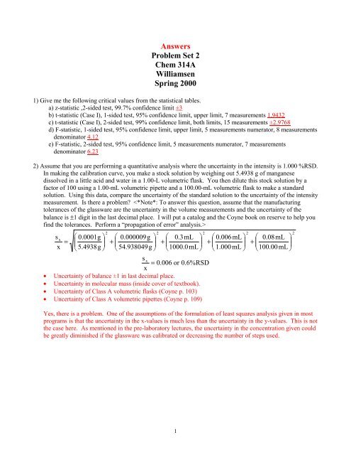
2) Assume that you are performing a quantitative analysis where the uncertainty in the intensity is 1.000 %RSD.
In making the calibration curve, you make a stock solution by weighing out 5.4938 g of manganese
dissolved in a little acid and water in a 1.00-L volumetric flask. You then dilute this stock solution by a
factor of 100 using a 1.00-mL volumetric pipette and a 100.00-mL volumetric flask to make a standard
solution. Using this data, compare the uncertainty of the standard solution to the uncertainty of the intensity
measurement. Is there a problem
s
x
=
x
0.0001g
5.4938g
2
+
0.000009g
54.938049g
2
+
s x
=
x
• Uncertainty of balance ±1 in last decimal place.
0.3mL
1000.0mL
0.006 or 0.6%RSD
• Uncertainty in molecular mass (inside cover of textbook).
• Uncertainty of Class A volumetric flasks (Coyne p. 103)
• Uncertainty of Class A volumetric pipettes (Coyne p. 109)
2
0.006 mL
+
1.000mL
2
+
0.08mL
100.00mL
Yes, there is a problem. One of the assumptions of the formulation of least squares analysis given in most
programs is that the uncertainty in the x-values is much less than the uncertainty in the y-values. This is not
the case here. As mentioned in the pre-laboratory lectures, the uncertainty in the concentration given could
be greatly diminished if the glassware was calibrated or decreasing the number of steps used.
2
1

3) You are performing a quantitative analysis to determine the concentration of Ca in a sample of seawater.
After determining that the other constituents of the seawater will not interfere with the analysis, you make a
calibration curve from intensity data measured while analyzing samples of known Ca concentration. Then you
analyze your sea water sample. After analyzing the results, you determine that the uncertainty about your
unknown concentration determination is too large.
a) State 4 ways in which you could decrease the uncertainty.
• Measure at more standard concentrations
• Make more measurements of the unknown
2
• Improve your technique to reduce s yx
• Have more standard concentrations near the
ends of the calibration curve
• Pick your standard concentrations so that the
unknown will be near the center of the
calibration line
b) Write the important equation(s) that helped you in determining how you can decrease the uncertainty and
show how your changes affect the values in this equation.
1−a
t
1
n− 2
N + 1 n + (y s
− y ) 2
b 2
x i
− x
i
( ) 2
2
s yx 2
s
b 2 yx
=
( y i
− y ˆ i
) 2
i
n − 2
• Measuring more standard concentrations (n) will decrease 1 n , will decrease t, and will decrease s 2
yx
( )
• More standard concentrations near the edges of the calibration curve will increase the x i
− x
• More measurements of the unknown will decrease 1 N
• Picking standard concentrations so the unknown will fall near the center of the calibration curve will
decrease y s
− y
( ) 2
2
• Improve your technique to reduce s yx
to reduce
( )
y i
− ˆ y i
4) One area of consideration when performing a hypothesis test is the setting of α- and β-error.
a) What are α- and β-errors Describe this in words and in pictures.
α-error is the chance of rejecting the null hypothesis when the null hypothesis is true, and β-error is the
chance of accepting the null hypothesis when the research hypothesis is true.
Values:
accept null
hypothesis
i
Values: accept
research
hypothesis
2
i
2
β
α
2

) How is the β-error set
The β-error is indirectly set by the α-error (which is directly set) and by the number of measurements.
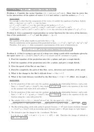
5) When determining the correct t-value to use in calculating the confidence limit of a number of measurements,
only one degree of freedom is lost, while when performing the calculation to determine the correct t-value to
use in calculating the confidence limit about a regression line, two degrees of freedom are lost. Why
One degree of freedom is lost when calculating the confidence limit about a measurement because the
sample mean is calculated. Two degrees of freedom are lost about the regression line are lost because two
statistics, the y-intercept and the slope, are calculated.
6) Most of the data sets that you will acquire during your lifetime will only be a sample of a population.
Although practical reasons often limit you to small number of points due to time constraints, statistical
theory tells us that under most conditions it is better to acquire more points. State why we would want to
obtain more data in each of the following cases. Use diagrams or expressions to support your reasoning, if
applicable.
a) Your data has a Poisson distribution, but you would like to analyze your data by performing an F-test.
One of the assumptions of the F-statistic is that the data is obtained from a normal distribution. The F-
statistic is not very robust so even data that is obtained from an “almost normal” distribution is suspect.
Although the data on which you wish to work follows the Poisson distribution, you can still use the
“normal distribution” statistics if the sample is large enough (n>30). The central limit theorem tells us
that no matter what the underlying distribution is, the data becomes more normally distributed as more
data is taken.
b) You are performing a hypothesis test and wish to reduce both the α- and β-error simultaneously.
One part of a hypothesis test is to set the α-level, which also sets the β-level. Without taking more data,
decreasing the β -level will increase the α -level and vice-versa. Taking more data will narrow the
distributions (decrease uncertainty) and therefore limit the values within the distribution that are outside
the set threshold(s).
c) You are performing a hypothesis test using the t-statistic and wish to accept the research hypothesis at
the 95% confidence limit.
The research hypothesis is accepted if the calculated t-value is larger than the absolute value of the
critical t-value. As the sample size increases, the critical t-value decreases. Also as more data is
acquired, the calculated t-value increases as t is proportional to n . Therefore, if there really is a bias,
the calculated t-value will eventually become larger than the critical t-value.
d) You can calculate the sample mean and wish to decrease the confidence limit of your estimate of the
population mean.
ts
The confidence limit of an estimate of the mean is given as . Therefore, as the number of data
n
points (n) increases, the confidence limits and uncertainty decrease.
7) Statistics for Analytical Chemists p. 80 Problem 6.
Answer p. 179.
Question: Is this spectroscopic method accurate
Statistic: t-test (Case I)
Level of significance: 95% confidence limit
Hypotheses (General form): H 0 : µ certified = x spectroscopic
H 1 : µ certified ≠ x spectroscopic
3

Experimental t-values:
Sample
Number t-statistic
1 1.54
2 1.60
3 1.18
4 1.60
Critical Value: t(0.95,7)=±2.36
Decision: Because all of the experimental t-statistics are within the critical limits, accept the null
hypothesis. The spectroscopically obtained values differ from the calibrated values by random variation
at the 95% confidence limit with 7 degrees of freedom. Therefore, the spectroscopic method appears to
accurately determine the value.
8) Statistics for Analytical Chemists p. 80 Problem 7.
Answer Chapter 3 p. 179. You would give the complete hypothesis test, I will only give you the
important values.
a) F-test (compare variances)
Experimental F: F=112 Critical value: F(0.95,7,7)=3.787 The decision would be that the longer boiling
point's variation is greater than can be explained by random variation at the 95% confidence limit with 8
measurements.
b) t-test (Case II) (compare means)
Experimental t: t=1.8 Critical value: t(0.95,14) )=±2.14

11) Mermet et al. Analytical Chemistry p 733 Problem 19.
Hypotheses: H 0 : s A =s B
H 1 : s A ≠s B
F=6.13 Because the calculated F-value is larger than the critical F-value, reject the null hypothesis.
The only statement that is true is that the hypothesis of method A being less precise than method B can not
be rejected. You did not directly test this hypothesis (that would be a 1-sided test), but because the
variances were found to be different, this hypothesis is not ruled out.
12) Mermet et al. Analytical Chemistry p 733 Problem 20.
Bullet 1:
Test: F-test
Level of significance: 95% confidence limit
Hypotheses:
H 0 : s field ≤s laboratory
H 1 : s field >s laboratory
Experiment F: 14.0
Decision: Because the experimental F-value is greater than the critical value, reject the null hypothesis.
Therefore at the 95% confidence level with 7 degrees of freedom for each measurement, the precision of
the laboratory method is significantly greater than the field method.
Bullet 2:
Test: t-test (Case II)
Level of significance: 95% confidence limit
Hypotheses: H 0 : 5.50=4.80
H 1 : 5.50≠4.80
Experimental t: 4.25
Critical t: t(0.95,14)=2.145
Decision: Because the experimental t-value is greater than the critical t-value, reject the null hypothesis.
Therefore at the 95% level of significance with 14 degrees of freedom, the means of the two
methods do differ significantly.
Last Revision: 4 March 2000 EJW
5