The Good Gain method for PI(D) controller tuning - TechTeach
The Good Gain method for PI(D) controller tuning - TechTeach
The Good Gain method for PI(D) controller tuning - TechTeach

Create successful ePaper yourself
Turn your PDF publications into a flip-book with our unique Google optimized e-Paper software.
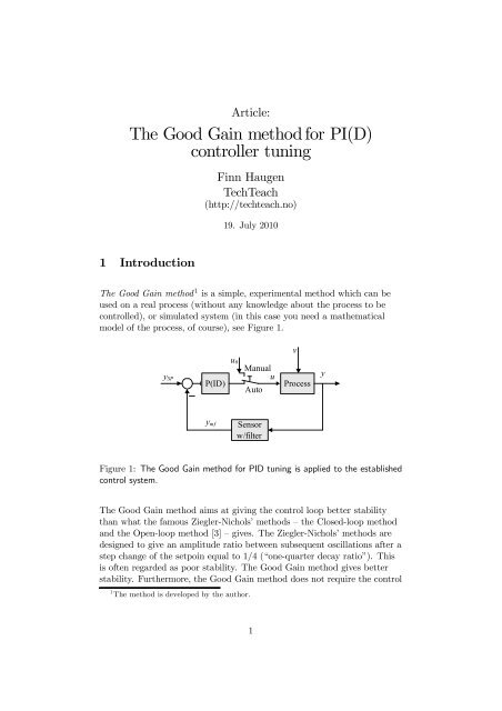
Article:<br />
<strong>The</strong> <strong>Good</strong> <strong>Gain</strong> <strong>method</strong> <strong>for</strong> <strong>PI</strong>(D)<br />
<strong>controller</strong> <strong>tuning</strong><br />
Finn Haugen<br />
<strong>TechTeach</strong><br />
(http://techteach.no)<br />
19. July 2010<br />
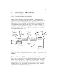
1 Introduction<br />
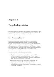
<strong>The</strong> <strong>Good</strong> <strong>Gain</strong> <strong>method</strong> 1 is a simple, experimental <strong>method</strong> which can be<br />
used on a real process (without any knowledge about the process to be<br />
controlled), or simulated system (in this case you need a mathematical<br />
model of the process, of course), see Figure 1.<br />
v<br />
y SP<br />
P(ID)<br />
u 0<br />
Manual<br />
u<br />
Auto<br />
Process<br />
y<br />
y mf<br />
Sensor<br />
w/filter<br />
Figure 1: <strong>The</strong> <strong>Good</strong> <strong>Gain</strong> <strong>method</strong> <strong>for</strong> <strong>PI</strong>D <strong>tuning</strong> is applied to the established<br />
control system.<br />
<strong>The</strong> <strong>Good</strong> <strong>Gain</strong> <strong>method</strong> aims at giving the control loop better stability<br />
than what the famous Ziegler-Nichols’ <strong>method</strong>s — the Closed-loop <strong>method</strong><br />
and the Open-loop <strong>method</strong> [3] — gives. <strong>The</strong> Ziegler-Nichols’ <strong>method</strong>s are<br />
designed to give an amplitude ratio between subsequent oscillations after a<br />
step change of the setpoin equal to 1/4 (“one-quarter decay ratio”). This<br />
is often regarded as poor stability. <strong>The</strong> <strong>Good</strong> <strong>Gain</strong> <strong>method</strong> gives better<br />
stability. Furthermore, the <strong>Good</strong> <strong>Gain</strong> <strong>method</strong> does not require the control<br />
1 <strong>The</strong> <strong>method</strong> is developed by the author.<br />
1
loop to get into oscillations during the <strong>tuning</strong>, which is another benefit<br />
compared with the Ziegler-Nichols’ <strong>method</strong>s.<br />
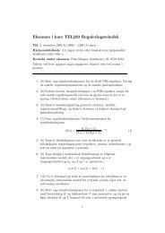
2 Tuning procedure<br />
<strong>The</strong> procedure described below assumes a <strong>PI</strong> <strong>controller</strong>, which is the most<br />
commonly used <strong>controller</strong> function. However, a comment about how to<br />
include the D-term, so that the <strong>controller</strong> becomes a <strong>PI</strong>D <strong>controller</strong>, is also<br />
given.<br />
1. Bring the process to or close to the normal or specified operation<br />
point by adjusting the nominal control signal u 0 (with the <strong>controller</strong><br />
in manual mode).<br />
2. Ensure that the <strong>controller</strong> is a P <strong>controller</strong> with K p = 0 (set T i = ∞<br />
and T d = 0). Increase K p until the control loop gets good<br />
(satisfactory) stability as seen in the response in the measurement<br />
signal after e.g. a step in the setpoint or in the disturbance (exciting<br />
with a step in the disturbance may be impossible on a real system,<br />
but it is possible in a simulator). If you do not want to start with<br />
K p = 0, you can try K p = 1 (which is a good initial guess in many<br />
cases) and then increase or decrease the K p value until you observe<br />
some overshoot and a barely observable undershoot (or vice versa if<br />
you apply a setpoint step change the opposite way, i.e. a negative<br />
step change), see Figure 2. This kind of response is assumed to<br />
represent good stability of the control system. This gain value is<br />
denoted K pGG .<br />
It is important that the control signal is not driven to any saturation<br />
limit (maximum or minimum value) during the experiment. If such<br />
limits are reached the K p value may not be a good one — probably<br />
too large to provide good stability when the control system is in<br />
normal operation. So, you should apply a relatively small step<br />
change of the setpoint (e.g. 5% of the setpoint range), but not so<br />
small that the response drowns in noise.<br />
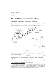
3. Set the integral time T i equal to<br />
T i = 1.5T ou (1)<br />
where T ou is the time between the overshoot and the undershoot of<br />
the step response (a step in the setpoint) with the P <strong>controller</strong>, see<br />
2
Figure 2. 2 Note that <strong>for</strong> most systems (those which does not containt<br />
a pure integrator) there will be offset from setpoint because the<br />
<strong>controller</strong> during the <strong>tuning</strong> is just a P <strong>controller</strong>.<br />
Setpoint step<br />
Step response in<br />
process<br />
measurement<br />
T ou<br />
T ou = Time<br />
between overshoot<br />
and undershoot<br />
Figure 2: <strong>The</strong> <strong>Good</strong> <strong>Gain</strong> <strong>method</strong>: Reading off the time between the overshoot<br />
and the undershoot of the step response with P <strong>controller</strong><br />
4. Because of the introduction of the I-term, the loop with the <strong>PI</strong><br />
<strong>controller</strong> in action will probably have somewhat reduced stability<br />
than with the P <strong>controller</strong> only. To compensate <strong>for</strong> this, the K p can<br />
be reduced somewhat, e.g. to 80% of the original value. Hence,<br />
K p = 0.8K pGG (2)<br />
5. If you want to include the D-term, so that the <strong>controller</strong> becomes a<br />
<strong>PI</strong>D <strong>controller</strong> 3 , you can try setting T d as follows:<br />
T d = T i<br />
4<br />
(3)<br />
which is the T d —T i relation that was used by Ziegler and Nichols [3].<br />
2 Alternatively, you may apply a negative setpoint step, giving a similar response but<br />
downwards. In this case T ou is time between the undershoot and the overshoot.<br />
3 But remember the drawbacks about the D-term, namely that it amplifies the measurement<br />
noise, causing a more noisy <strong>controller</strong> signal than with a <strong>PI</strong> <strong>controller</strong>.<br />
3
6. You should check the stability of the control system with the above<br />
<strong>controller</strong> settings by applying a step change of the setpoint. If the<br />
stability is poor, try reducing the <strong>controller</strong> gain somewhat, possibly<br />
in combination with increasing the integral time.<br />
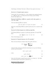
Eksempel 1 <strong>PI</strong> <strong>controller</strong> <strong>tuning</strong> of a wood-chip level control<br />
system with the <strong>Good</strong> <strong>Gain</strong> Method<br />
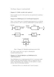
I have tried the Ziegler-Nichols’ closed loop <strong>method</strong> on a level control<br />
system <strong>for</strong> a wood-chip tank with feed screw and conveyor belt which runs<br />
with constant speed, see Figure 3. 4 5 <strong>The</strong> purpose of the control system is<br />
to keep the chip level of the tank equal to the actual, measured level.<br />
<strong>The</strong> level control system works as follows: <strong>The</strong> <strong>controller</strong> tries to keep the<br />
measured level equal to the level setpoint by adjusting the rotational speed<br />
of the feed screw as a function of the control error (which is the difference<br />
between the level setpoint and the measured level).<br />
During the <strong>tuning</strong> I found<br />
and<br />
<strong>The</strong> <strong>PI</strong> parameter values are<br />
K pGG = 1.5 (4)<br />
T ou = 12 min (5)<br />
K p = 0.8K pGG = 0.8 · 1.5 = 1.2 (6)<br />
T i = 1.5T ou = 1.5 · 12 min = 18 min = 1080 s (7)<br />
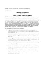
Figure 4 shows the resulting responses with a setpoint step at time 20 min<br />
and a disturbance step (outflow step from 1500 to 1800 kg/min) at time<br />
120 min. <strong>The</strong> control system has good stability.<br />
[End of Example 1]<br />
3 <strong>The</strong>oretical background<br />
In the <strong>Good</strong> <strong>Gain</strong> <strong>method</strong> the process is controlled with a P-<strong>controller</strong>,<br />
and the step response in the process output due to a step in the setpoint is<br />
4 This example is based on an existing system in the paper pulp factory Södra Cell Tofte<br />
in Norway. <strong>The</strong> tank with conveyor belt is in the beginning of the paper pulp production<br />
line.<br />
5 A simulator of the system is available at http://techteach.no/simview.<br />
4
Process & Instrumentation (P&I) Diagram:<br />
Process (tank with belt and screw)<br />
Feed screw<br />
Conveyor<br />
belt<br />
Wood chip<br />
u<br />
Control<br />
variable<br />
Level<br />
<strong>controller</strong><br />
LC<br />
y SP<br />
Reference<br />
or<br />
Setpoint<br />
y m<br />
Process<br />
measurement<br />
Sensor Process<br />
(Level output<br />
transmitter) variable<br />
y [m]<br />
LT<br />
n<br />
Measurement<br />
noise<br />
Wood<br />
chip tank<br />
Process disturbance<br />
(environmental variable)<br />
d [kg/min]<br />
Block diagram:<br />
Reference<br />
or<br />
Setpoint<br />
y SP<br />
Level <strong>controller</strong> (LC)<br />
Control<br />
error<br />
e<br />
<strong>PI</strong>D<br />
<strong>controller</strong><br />
Control<br />
variable<br />
u<br />
Process disturbance<br />
(environmental variable)<br />
d<br />
Process output<br />
Process variable<br />
(tank with y<br />
belt and<br />
screw)<br />
y m,f<br />
Filtered<br />
measurement<br />
Process<br />
measurement<br />
Measurement<br />
filter<br />
y m<br />
Sensor<br />
(Level<br />
Transmitter<br />
- LT)<br />
n<br />
Control<br />
loop<br />
Measurement<br />
noise<br />
Figure 3: P&I (Process and Instrumentation) diagram and block diagram of a<br />
level control system <strong>for</strong> a wood-chip tank in a pulp factory<br />
well-damped oscillations. Let’s assume that the control loop behaves<br />
approximately as an underdamped second order system with the following<br />
transfer function model from setpoint to process output:<br />
y(s)<br />
y SP (s) = Kω 2 0<br />
s 2 + 2ζω 0 s + ω 2 0<br />
(8)<br />
It can be shown that with ζ = 0.6 the step response is damped oscillations<br />
with an overshoot of about 10% and a barely observable undershoot, as in<br />
5
Figure 4: Example 1: Level control of the wood-chip tank with a <strong>PI</strong> <strong>controller</strong>.<br />
the <strong>Good</strong> <strong>Gain</strong> <strong>tuning</strong>, and that the period of the damped oscillations is<br />
P d =<br />
=<br />
2π<br />
√<br />
1 − ζ 2 ω 0<br />
=<br />
2π<br />
√<br />
1 − 0.6 2 ω 0<br />
(9)<br />
2π<br />
0.8ω 0<br />
= P GG = 2T ou (10)<br />
If the oscillations are undamped, as with the Ziegler-Nichols’ Ultimate<br />
<strong>Gain</strong> <strong>method</strong>, the period of the oscillations is<br />
P ZN = 2π<br />
ω 0<br />
(11)<br />
Hence, the relation between the period of the damped oscillations of the<br />
<strong>Good</strong> <strong>Gain</strong> <strong>method</strong> and the undamped oscillations of the Ziegler-Nichols’<br />
<strong>method</strong> is approximately<br />
In the Ziegler-Nichols’ <strong>method</strong> we set<br />
P ZN = 0.8P GG = 1.6T ou (12)<br />
T i = P ZN<br />
1.2 = 1.6T ou<br />
1.2<br />
= 1.33T ou (13)<br />
If we make the T i setting somewhat more relaxed (to obtain better<br />
stability and better robustness), we can increase T i to<br />
T i = 1.5T ou (14)<br />
In the Ziegler-Nichols’ <strong>method</strong> the <strong>controller</strong> gain K c of a <strong>PI</strong>-<strong>controller</strong> is<br />
90% of the gain of the P-<strong>controller</strong>. To compensate <strong>for</strong> the inclusion of the<br />
integral term we can reduce the original <strong>controller</strong> gain of the <strong>Good</strong> <strong>Gain</strong><br />
<strong>method</strong> to 90%, but to relax the setting even more, let’s set<br />
K c = 0.8K cGG (15)<br />
6
Note that the <strong>Good</strong> <strong>Gain</strong> <strong>method</strong> can not be used if the process transfer<br />
function (from control signal u to filtered process measurement y mf ) is one<br />
of the following:<br />
• Integrator without delay:<br />
H p (s) = y mf(s)<br />
u(s)<br />
• Time-constant without time-delay:<br />
= K s<br />
(16)<br />
H p (s) =<br />
K<br />
T s + 1<br />
(17)<br />
This is because with the above process models, there will be no oscillations<br />
in the response in the process output due to a step in the setpoint, with a<br />
P-<strong>controller</strong>.<br />
One example of an integrator without time-delay is a liquid tank where<br />
level is to be controlled and the <strong>controller</strong> adjusts the inflow, and there is<br />
outflow via a pump. If the outflow is via a valve, the model will<br />
approximately be a time-constant transfer function.<br />
For processes like (16) and (17) you can tune the <strong>controller</strong> with<br />
Skogestad’s <strong>method</strong> [2], which is summarized in the text-book Basic<br />
Dynamics and Control [1].<br />
References<br />
[1] Haugen, F.: Basic Dynamics and Control, <strong>TechTeach</strong><br />
(http://techteach.no) 2010<br />
[2] Skogestad, S.: Simple Analytical Rules <strong>for</strong> Model Reduction and <strong>PI</strong>D<br />
Controller Tuning, J. Process Control, Vol. 13, 2003<br />
[3] Ziegler, J. G. and Nichols, N. B.: Optimum Settings <strong>for</strong> Automatic<br />
Controllers, Trans. ASME, Vol. 64, 1942, s. 759-768<br />
7