Finn Haugen, TechTeach: Exercises to Discrete-time signals and ...
Finn Haugen, TechTeach: Exercises to Discrete-time signals and ...
Finn Haugen, TechTeach: Exercises to Discrete-time signals and ...
- No tags were found...

Create successful ePaper yourself
Turn your PDF publications into a flip-book with our unique Google optimized e-Paper software.
<strong>Finn</strong> <strong>Haugen</strong>, <strong>TechTeach</strong>: <strong>Exercises</strong> <strong>to</strong> <strong>Discrete</strong>-<strong>time</strong> <strong>signals</strong> <strong>and</strong> systems 1Exercise 0.1 Sampled signal sequenceAssume that a the ramp signal r(t) =Rt is sampled with sampling frequencyf s =10Hz from <strong>time</strong> t =0.Writethefirst five values of the resultingdiscrete-<strong>time</strong> signal r d (t k ).Exercise 0.2 Writing a difference equation with only negative orzero <strong>time</strong> shiftsGiven the following difference equation:y(k +3)+ay(k +1)=b 1 u(k +2)+b 0 u(k) (1)Write the corresponding difference equation having only zero or negative <strong>time</strong>shifts.Exercise 0.3 Block diagram of a filtering algorithmThe following difference equation is the filtering algorithm of a simple FIR 1filter:y(k) = 1 [u(k)+u(k − 1) + u(k − 2)] (2)3Draw a block diagram of (2).Exercise 0.4 Transfer function of a PI controllerHere is the <strong>time</strong>-domain continuous-<strong>time</strong> PI controller function:Z tu(t) =K p e(t) + K pedt(3)| {z } T i 0u p| {z }u iUsing the Euler backward method for discretizing (3), we get the followingdiscrete-<strong>time</strong> PI controller:u(k) =u p (k)+u i (k) (4)whereu p (k) =K p e(k) (5)u i (k) =u i (k − 1) + K phe(k) (6)T iDerive the PI controller transfer function (from e <strong>to</strong> u) from (4) — (6). Writethe transfer function with positive exponents of z.Exercise 0.5 Poles <strong>and</strong> zeros1 FIR = Finite Impulse Response
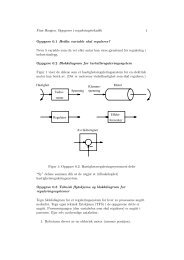
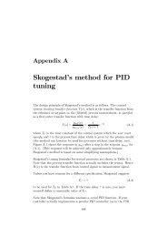
<strong>Finn</strong> <strong>Haugen</strong>, <strong>TechTeach</strong>: <strong>Exercises</strong> <strong>to</strong> <strong>Discrete</strong>-<strong>time</strong> <strong>signals</strong> <strong>and</strong> systems 2Given the following transfer function:H(z) = bz−2 + z −11 − az −1 (7)Calculate the poles <strong>and</strong> the zeros of the transfer function.Exercise 0.6 Stability analysis of numerical algorithmDiscretizing the continuous-<strong>time</strong> transfer functionH con (s) = y(s)u(s) = KTs+1(8)using Euler’s forward method with <strong>time</strong>-step h yields the followingdiscrete-<strong>time</strong> transfer function:H dis (z) = y(z)u(z) =KhTz − ¡ 1 − h T¢ (9)For which (positive) values of h is the discrete-<strong>time</strong> system asymp<strong>to</strong>ticallystable? (You can assume that T is positive.)Exercise 0.7 Setting up the sensitivity transfer function of a controlsystemFigure 1 shows a block diagram of a feedback control system.• What is the loop transfer function L(z) of the control system?• What is the sensivity transfer function S(z)?• What is the tracking transfer function T (s)?Exercise 0.8 Stability analysis in a Bode diagramFigure 2 shows the Bode curves of the loop transfer function of a given controlsystem.What are the stability margins GM <strong>and</strong> PM, <strong>and</strong> the crossover frequencies ω c<strong>and</strong> ω 180 ?
<strong>Finn</strong> <strong>Haugen</strong>, <strong>TechTeach</strong>: <strong>Exercises</strong> <strong>to</strong> <strong>Discrete</strong>-<strong>time</strong> <strong>signals</strong> <strong>and</strong> systems 3ProcessdisturbanceProcessd(s)Setpointy SP (z)H s (z)Model ofsensor withscalingSetpointin measurementunity mSP (z)Controlerrore m (z)Hc (z)ControllerMeasurementControlvariableu(z)y m (z)H u (z)H d (z)Actua<strong>to</strong>rtransfer functionH s (z)Sensor(measurement)with scalingDisturbancetransfer functiony(z)ProcessoutputvariableFigure 1: Exercise 0.7: Feedback control systemSolution 0.1Thesampling<strong>time</strong>orintervalish = 1 = 1 =0.1s (10)f s 10Since t k = kh,r d (t k )=Rt k = Rkh (11)The first five values corresponds <strong>to</strong> k =0,..,4, i.e.{0, Rh, R2h, R3h, R4h} (12)or{0, 0.1R, 0.2R, 0.3R, 0.4R} (13)Solution 0.2Each of the <strong>time</strong> indexes is reduced by 3, <strong>to</strong> givey(k)+ay(k − 2) = b 1 u(k − 1) + b 0 u(k − 3) (14)Solution 0.3Figure 3 shows the block diagram.Solution 3Taking the z-transform of (4) — (6) givesu(z) =u p (z)+u i (z) (15)
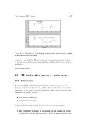
<strong>Finn</strong> <strong>Haugen</strong>, <strong>TechTeach</strong>: <strong>Exercises</strong> <strong>to</strong> <strong>Discrete</strong>-<strong>time</strong> <strong>signals</strong> <strong>and</strong> systems 4Figure 2: Exercise 0.8: Bode plots of control systemwhereu p (z) =K p e(z) (16)u i (z) =z −1 u i (z)+ K phe(z) (17)T iFrom (17) we solve for u i (z) <strong>to</strong> getu i (z) = K ph/T ie(z) (18)1 − z−1 Inserting (16) <strong>and</strong> (18) in<strong>to</strong> (15) yieldsu(z) = u p (z)+u i (z) (19)= K p e(z)+ K ph/T ie(z) (20)1 − z−1 = (K p + K p h/T i ) − K p z −11 − z −1 e(z) (21)= (K p + K p h/T i ) z − K pe(z) (22)z − 1
<strong>Finn</strong> <strong>Haugen</strong>, <strong>TechTeach</strong>: <strong>Exercises</strong> <strong>to</strong> <strong>Discrete</strong>-<strong>time</strong> <strong>signals</strong> <strong>and</strong> systems 5u(k)z -1u(k-1)z -1u(k-2)1/3y(k)Figure 3: Solution 0.3: Block diagramThus, the transfer function isH c (z) = u(z)e(z) = (K p + K p h/T i ) z − K pz − 1(23)Solution 0.5It is convenient <strong>to</strong> start by rewriting the transfer function as follows:Thus, the zero ζ is<strong>and</strong> the poles p i areH(z) = z−2 b + z −11 − az −1 · z2z 2 =z + bz 2 − az =z + b(z − a) z(24)ζ = −b (25)p 1 = a; p 2 =0 (26)Solution 0.6Thepoleof(9)isp =1− h T(27)The system is asymp<strong>to</strong>tically stable if¯¯p =1− h T ¯ < 1 (28)If(28) becomeswhich gives1 − h T > 0 (29)1 − h T < 1 (30)h>0 (31)
<strong>Finn</strong> <strong>Haugen</strong>, <strong>TechTeach</strong>: <strong>Exercises</strong> <strong>to</strong> <strong>Discrete</strong>-<strong>time</strong> <strong>signals</strong> <strong>and</strong> systems 6which is always satisfied.If(28) becomes1 − h T < 0 (32)µ− 1 − h < 1 (33)Twhich givesh< T 2(34)Solution 0.71. The loop transfer function is the product of the transfer functions in theloop:L(z) =H c (z)H u (z)H s (z) (35)2. The sensitivity transfer function isS(z) =11+L(z) = 11+H c (z)H u (z)H s (z)(36)3. The tacking transfer function isT (z) =L(z)1+L(z) = H c(z)H u (z)H s (z)1+H c (z)H u (z)H s (z)(37)Solution 0.8From the Bode diagram shown in Figure 2 we read offGM =7dB =2.2 (38)PM =35 ◦ (39)ω c =0.34rad/s (40)ω 180 =0.58rad/s (41)