4.9 PID tuning when process dynamics varies - TechTeach

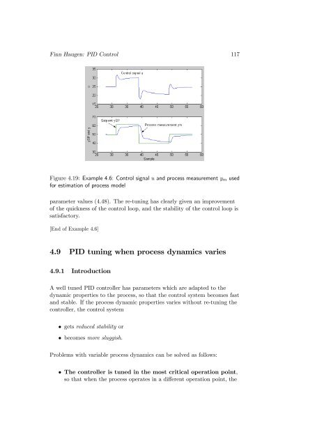
Finn Haugen: PID Control 117Figure 4.19: Example 4.6: Control signal u and process measurement y m usedfor estimation of process modelparameter values (4.48). The re-tuning has clearly given an improvementof the quickness of the control loop, and the stability of the control loop issatisfactory.[End of Example 4.6]4.9 PID tuning when process dynamics varies4.9.1 IntroductionA well tuned PID controller has parameters which are adapted to thedynamic properties to the process, so that the control system becomes fastand stable. If the process dynamic properties varies without re-tuning thecontroller, the control system• gets reduced stability or• becomes more sluggish.Problems with variable process dynamics can be solved as follows:• The controller is tuned in the most critical operation point,so that when the process operates in a different operation point, the

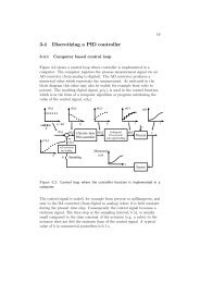
118 Finn Haugen: PID ControlFigure 4.20: Example 4.6: Response in process output for control system withoriginalandre-tunedPIcontrollerparametersstability of the control system is just better – at least the stability isnot reduced. However, if the stability is too good the trackingquickness is reduced, giving more sluggish control.• The controller parameters are varied in the “opposite”direction of the variations of the process dynamics, sothatthe performance of the control system is maintained, independent ofthe operation point. Two ways to vary the controller parameters are:— PID controller with gain scheduling. This is described in detailin Section 4.9.2.— Model-based adaptive controller. This is described briefly inSection 4.9.4.Commercial control equipment is available with options for gain schedulingand/or adaptive control.4.9.2 Gain scheduling PID controllerFigure 4.21 shows the structure of a control system for a process whichmay have varying dynamic properties, for example a varying gain. TheGain scheduling variable GS is some measured process variable which atevery instant of time expresses or represents the dynamic properties of theprocess. As you will see in Example 4.7, GS may be the mass flow throughaliquidtank.

Finn Haugen: PID Control 119Adjustment ofcontrollerparametersGS GainschedulingvariableSetpointControllerProcess withvaryingdynamicpropertiesSensorandscalingFigure 4.21: Control system for a process having varying dynamic properties.The GS variable expresses or represents the dynamic properties of the process.Assume that proper values of the PID parameters K p , T i and T d are foundusing for example Ziegler-Nichols’ closed loop method for a set of values ofthe GS variable. These PID parameter values can be stored in a parametertable — the gain schedule — as shown in Table 4.3. From this table properPID parameters are given as functions of the gain scheduling variable, GS.GS K p T i T dP 1 K p1 T i1 T d1P 2 K p2 T i2 T d2P 3 K p3 T i3 T d3Table 4.3: Gain schedule or parameter table of PID controller parameters.There are several ways to express the PID parameters as functions of theGS variable:• Piecewise constant controller parameters: Anintervalisdefined around each GS value in the parameter table. The controllerparameters are kept constant as long as the GS value is within theinterval. This is a simple solution, but is seems nonetheless to be themost common solution in commercial controllers.When the GS variable changes from one interval to another, thecontroller parameters are changed abruptly, see Figure 4.22 whichillustrates this for K p , but the situation is the same for T i and T d .In

120 Finn Haugen: PID ControlFigure 4.22 it is assumed that GS values toward the left are criticalwith respect to the stability of the control system. In other words: Itis assumed that it is safe to keep K p constant and equal to the K pvalue in the left part of the the interval.K pTable values of K pK p3K p2K p1Linear interpolationPiecewise constant value(with hysteresis )GS 1 GS 2 GS 3 GSAssumed range of PFigure 4.22: Two different ways to interpolate in a PID parameter table: Usingpiecewise constant values and linear interpolationUsing this solution there will be a disturbance in the form of a stepin the control variable when the GS variable shifts from one intervalto a another, but this disturbance is probably of negligible practicalimportance for the process output variable. Noise in the GS variablemay cause frequent changes of the PID parameters. This can beprevented by using a hysteresis, as shown in Figure 4.22.• Piecewise interpolation, which means that a linear function isfound relating the controller parameter (output variable) and the GSvariable (input variable) between to adjacent sets of data in thetable. The linear function is on the formK p = a · GS + b (4.49)where a and b are found from the two corresponding data sets:K p1 = a · GS 1 + b (4.50)K p2 = a · GS 2 + b (4.51)

Finn Haugen: PID Control 121(Similar equations applies to the T i parameter and the T dparameter.) (4.50) and (4.51) constitute a set of two equations withtwo unknown variables, a and b. 8• Other interpolations may be used, too, for example a polynomialfunction fitted exactly to the data or fitted using the least squaresmethod.Example 4.7 Gain schedule based PID temperature control atvariable mass flowFigure 4.25 shows the front panel of a simulator for a temperature controlsystem for a liquid tank with variable mass flow, w, through the tank. Thecontrol variable u controls the power to heating element. The temperatureT is measured by a sensor which is placed some distance away from theheating element. There is a time delay from the control variable tomeasurement due to imperfect blending in the tank.The process dynamics We will initially, both in simulations and fromanalytical expressions, that the dynamic properties of the process varieswith the mass flow w. The response in the temperature T is simulated forthe following two open loop cases (i.e., not feedback control):• A step in u of amplitude 10% from 31.5% to 41.5% at mass floww =12kg/min, which in this context is a relatively small value, seeFigure 4.23.• A step in u of amplitude 10%, from 63.0 % to 73.0 % atw =24kg/min, which in this context is a relatively large value, seeFigure 4.24.The simulations show that the following happens when the mass flow w isreduced (from 24 to 12kg/min): The gain process K is larger, the timeconstant T t is larger, and the time delay τ is larger. (These terms assumesthat system is a first order system with time delay. The simulator is basedon such a model. The model is described below.)Let us see if the way the process dynamics seems to depend on the massflow w as seen from the simulations, can be confirmed from a8 The solution is left to you.

122 Finn Haugen: PID ControlFigure 4.23: Response in temperature T after a step in u of amplitude 10%from 31.5% to 41.5% at the small mass flow w =12kg/minFigure 4.24: Response in temperature T after a step in u of amplitude 10%from 63.0% to 73.0% at the large mass flow w =24kg/minmathematical process model. 9 Assuming perfect stirring in the tank tohave homogeneous conditions in the tank, we can set up the followingenergy balance for the liquid in the tank:cρV ˙ T 1 (t) =K P u(t)+cw [T in (t) − T t (t)] (4.52)where T 1 [K] is the liquid temperature in the tank, T in [K] is the inlettemperature, c [J/(kg K)] is the specific heat capacity, V [m 3 ] is the liquidvolume, ρ [kg/m 3 ] is the density, w [kg/s] is the mass flow (same out asin), K P [W/%] is the gain of the power amplifier, u [%] is the controlvariable, cρVT 1 is (the temperature dependent) energy in the tank. It isassumed that the tank is isolated, that is, there is no heat transfer through9 Well, it would be strange if not. After all, we will be analyzing the same model asused in the simulator.

Finn Haugen: PID Control 123thewallstotheenvironment.Tomakethemodelalittlemorerealistic,wewill include a time delay τ [s] to represent inhomogeneous conditions in thetank. Let us for simplicity assume that the time delay is inverselyproportional to the mass flow. Thus, the temperature T at the sensor isT (t) =T 1 (t − K τ) (4.53)|{z} wτwhere τ isthetimedelayandK τ is a constant. Let us study the transferfunction from u to T . Taking the Laplace transform of (4.52) givescρV [sT 1 (s) − T 10 ]=K P u(s)+cw [T in (s) − T t (s)] (4.54)where T 10 is the initial value of T . Rearranging (4.54) yields the followingmodelT 1 (s) =ρVwK PcwρVρVw s +1T 1 0+Taking the Laplace transform of (4.53) gives1w s +1u(s)+ ρVw s +1T in(s) (4.55)T (s) =e − K τs w T 1 (s) (4.56)Substituting T 1 (s) in (4.56) by T 1 (s) from (4.55) yields the followingtransfer function H u (s) from u to T :T (s) =Kz}|{K PcwρVs +1|{z} wT te −τz}|{K τw s u(s) (4.57)=KT t s +1 e−τs u(s)| {z }(4.58)H u(s)Thus,K = K Pcw(4.59)T t = ρV w(4.60)τ = K τw(4.61)This confirms the observations in the simulations: Reduced mass flow wimplies larger process gain, larger time constant, and larger time delay.Heat exchangers and blending tanks in a process line where the productionrate or mass flow varies, have similar dynamic properties as the tank inthis example.

124 Finn Haugen: PID ControlFigure 4.25: Example 4.7: Simulation of temperature control system with PIDcontroller with fixed parameters tuned at maximum mass flow, which is w =24kg/minControl without gain scheduling (with fixed parameters) Let uslook at temperature control of the tank. The mass flow w varies. In whichoperating point should the controller be tuned if we want to be sure thatthe stability of the control system is not reduced when w varies? In generalthe stability of a control loop is reduced if the gain increases and/or if thetime delay of the loop increases. (4.59) and (4.61) show how the gain andtime delay depends on the mass flow w. According to (4.59) and (4.61) thePID controller should be tuned at minimal w. If we do the opposite, thatis, tune the controller at the maximum w, the control system may actuallybecome unstable if w decreases.Let us see if a simulation confirms the above analysis. Figure 4.25 shows atemperature control system. The PID controller is in the example tunedwith the Ziegler-Nichols’ closed loop method for a the maximum w value,

Finn Haugen: PID Control 125which here is assumed 24kg/min. The PID parameters areK p =7.8; T i =3.8min; T d =0.9min (4.62)Figure 4.25 shows what happens at a stepwise reduction of w: Thestability becomes worse, and the control system becomes unstable at theminimal w value, which is 12kg/min.Instead of using the PID parameters tuned at maximum w value, we cantune the PID controller at minimum w value, which is 12kg/min. Theparameters are thenK p =4.1; T i =7.0min; T d =1.8min (4.63)The control system will now be stable for all w values, but the systembehaves sluggish at large w values. (Responses for this case is however notshown here.)Control with gain scheduling Let us see if gain scheduling maintainsthe stability for varying mass flow w. The PID parameters will be adjustedas a function of a measurement of w since the process dynamics varies withw. Thus,w is the gain scheduling variable, GS:GS = w (4.64)A gain schedule consisting of three PID parameter value sets will be used.Each set is tuned using the Ziegler-Nichols’ closed loop method at thefollowing GS or w values: 12, 16 and 20kg/min. These three PIDparameter sets are shown down to the left in Figure 4.25. The PIDparameters are held piecewise constant in the GS intervals. In eachinterval,thePIDparametersareheldfixed for an increasing GS = wvalue, cf. Figure 4.22. 10 Figure 4.26 shows the response in the temperaturefor decreasing values of w. The simulation shows that the stability of thecontrol system is maintained even if w decreases.[End of Example 4.7]4.9.3 Adjusting PID parameters from process modelIn Section 4.9.2 the adjustment of the PID parameters was based oninterpolating between PID parameter values in a parameter table.However, a table with interpolation is not the only way the adjustment can10 The simulator uses the inbuilt gain schedule in LabVIEW’s PID Control Toolkit.

126 Finn Haugen: PID ControlFigure 4.26: Example 4.7: Simulation of temperature control system with again schedule based PID controllerbe implemented. By studying the process model we may find a function forparameter adjustment without having to make tuning in a number ofoperating points. Assume as an example that the process gain K is afunction of a process variable P :K = f K (P ) (4.65)In many control loops the stability of the loop is maintained if the loopgain K L , which is the product of the gain of each subsystems in the loop,is constant, say K L0 . In other words, the stability is maintained ifK L = K p KK s = K p f K (P ) K s = K L0 (4.66)where K p is the controller gain (of a P or PI or PID controller) and K m isthe measurement gain (including a scaling function). For a given P value,

Finn Haugen: PID Control 127say P 1 ,K p1 f K (P 1 ) K s = K L0 (4.67)where K p1 is assumes to be a proper K p value (found using some tuningmethod) when P = P 1 . By dividing (4.66) by (4.67) we getK p f K (P ) K s= K L 0=1 (4.68)K p1 f K (P 1 ) K s K L0from which we get the following formula for adjusting the controller gainK p :f K (P 1 )K p = K p1 (4.69)f K (P )Adjusting K p according to (4.69) ensures that the stability of the controlloop is maintained for any P value.Example 4.8 Model based adjustment of level controllerFigure 4.27 shows a level control system for a cylindrical tank.You willw inρhARmLT0VLPIcontrollerLCuw out=K uuFigure 4.27: Example 4.8: Level control of a cylindric tank. The cross sectionalarea is a function of the level.now see that the process gain K varies with the level. This implies thatthe controller gain K p should vary. Mass balance for the liquid of the tank(we assume homogeneous conditions) isdmdt = ρdV dt = ρAdh dt = w in − w out = w in − K u u (4.70)

128 Finn Haugen: PID ControlIt can be shown that the cross sectional area A is a function of the level has follows:A(h) =2L p R 2 − (R − h) 2 (4.71)From (4.70) we find that the transfer function from a deviation ∆u in thecontrol signal to the corresponding deviation ∆h in the level is 11∆h(s)∆u(s)u= H(s) =−K ρA(h)s(4.72)giving the following process gainK uK = − K uρA(h) = −2ρL p R 2 − (R − h) = f K(h) (4.73)2The controller gain should be adjusted according to (4.69), which in thiscase givesh if K (h 1 ) −KuK p = K p1f K (h) = K ρA(h 1 ) A(h)p 1h i = K− K p1(4.74)u A(h 1 )ρA(h)where f K is given by (4.73) and A(h) is given by (4.71). K p1 is a K p valueof a P or PI controller (the PID controller is not a good choice for thislevel control system since the process has pure integrator dynamics) tunedat some level h 1 .(Forexample,h 1 may correspond to half of the maximumlevel.) K p can be found by trial and error, or better: from transferfunction based controller tuning, cf. Chapter 7. For example, (4.74) saysthat if the cross sectional area is halved (which gives doubled processgain), K p should be halved. The integral time T i in a PI controller can beunchanged in this case.[End of Example 4.8]4.9.4 Adaptive controllerIn an adaptive control system, see Figure 4.28, a mathematical model ofthe process to be controlled is continuously estimated from samples of thecontrolsignal(u) and the process measurement (y m ). The model istypically a transfer function model. Typically, the structure of the model isfixed. The model parameters are estimated continuously using e.g. theleast squares method. From the estimated process model the parameters ofa PID controller (or of some other control function) are continuously11 The transfer function is here actually relating the deviation variables about an operatingpoint since the process model is nonlinear.

Finn Haugen: PID Control 129Continuouslycalculation ofcontrollerparametersContinuouslyprocess modelestimationy SPeControlleruvProcessyy mSensorandscalingFigure 4.28: Adaptive control systemcalculated so that the control system achieves specified performance inform of for example stability margins, poles, bandwidth, or minimumvariance of the process output variable[22]. Adaptive controllers arecommercially available, for example the ECA60 controller (ABB).