Finn Haugen: Exercises to Dynamic Systems 1 ... - TechTeach

Finn Haugen: Exercises to Dynamic Systems 1
Exercise 1 Chip tank
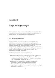
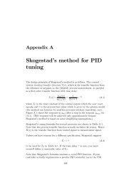
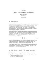
Figure 1 shows a chip tank with a feed screw and conveyor belt (the belt
has constant speed). 1 There is an outflow of chip via an outlet at the
Screw constant
K s [(kg/min)/mA]
Feed screw
Mass flow
w s [kg/min]
Time delay
τ [min]
Conveyor belt
w in [kg/min]
Chip
Screw control
signal
u [mA]
Chip tank
Chip
Level
h [m]
Chip density
ρ [kg/m 3 ]
A [m 2 ]
0 m
w out [kg/min]
To the
cookery
Figure 1: Exercise 1: Chip tank with a feed screw and conveyor belt
bottom of the tank. The mass flow w s from the feed screw to the belt is
proportional to the screw control signal u:
w s = K s u (1)
The mass flow w in into the chip tank is equal to w s but time delayed time
τ:
w in (t) =w s (t − τ) (2)
1. Develop a mathematical model of the chip level.
2. Draw an input-output block diagram of the system. Define the input
and output variables, but it is assumed that the level is of particular
interest.
Exercise 2 Heated tank
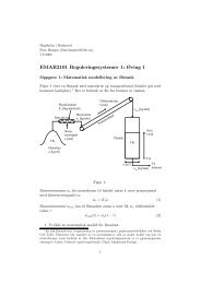
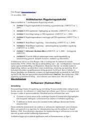
Figure2showsaheatedtankwithliquidflow. Both the liquid in the tank
1 Typically, there is such a chip tank in the beginning of the production line of a paper
mass factory.

2 Finn Haugen: Exercises to Dynamic Systems
Specific heating capacity
c [J/(kg K)]
Mass flow
w [kg/s]
Heat transfer
coefficient
U [(J/s)/K]
Environmental
temperature
T env [K]
Inlet temperature
T in [K]
Density
ρ [kg/m 3 ]
Heating transfer
coefficient
U h [(J/s)/K]
Heating capacity
C h [J/K]
Mixer
V [m 3 ]
T [K]
Supplied
power
P [J/s]
w
T
Heating element
temperature
T h [K]
Figure 2: Exercise 2: Heated tank with liquid flow
and the heating element have heat capacities. The heat transfer between
the environment and the liquid is proportional to the temperature
difference between them. The heat transfer between the heating element
and the liquid is also proportional to the temperature difference between
them. Assume homogenous conditions.
1. Develop a mathematical model of the temperatures of the liquid in
the tank and the heating elementet.
2. Draw an input-output block diagram of the system. Consider then
P , T o , T i and w as input variables and T as an output variable.
Exercise 3 Ship model
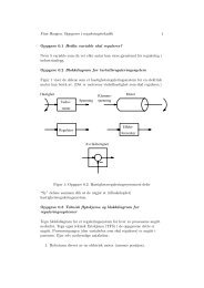
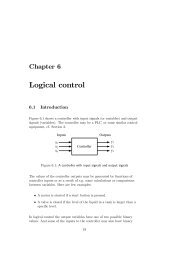
Figure 3 shows a ship. In this exercise we concentrate on the forward
direction (i.e., the movements in the other directions are disregarded). The
wind acts on the ship with the force F w . The hydrodynamic damping force
F h (damping from the water) is proportional to the square of the difference
between the ship speed u and the water current speed u c . Assume that the
proportionality constant is D x .

Finn Haugen: Exercises to Dynamic Systems 3
W ind force
F w [N ]
P ropeller force
F p [N ]
M ass m [kg]
H ydrodynamic
force F h [N ]
P o sitio n x [m ]
Ship speed (relative to earth ) u [m /s]
W ater cu rren t sp eed (rel. to earth ) u c
[m /s]
Figure 3: Exercise 3: A ship
1. What is the mathematical relation between speed u and position x
2. Develop a mathematical model of the ship expressing the motion
(the position) in the forward direction.
3. Draw an input-output block diagram of the system. Assume that the
ship position is the variable of particular interest.

4 Finn Haugen: Exercises to Dynamic Systems
Solution 1
1. Since there is a time delay in the system (due to the transport delay
of the conveyor belt) it is important to inlcude the time argument in
the equations. The mass balance if the chip contents of the tank is
d
dt [ρAh(t)] = ρAḣ(t) = w in(t) − w out (t)
= w s (t − τ) − w out (t)
= K s u(t − τ) − w out (t)
(3)
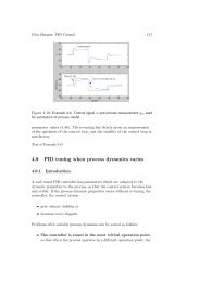
2. Figure 4 shows the block diagram.
u
w out
Chip tank
with conveyor
belt
h
Figure 4: Solution 1: Block diagram of chip tank with conveyor belt
Solution 2
1. Energy balance of the liquid in the tank:
d(cρVT)
dt
= cρV ˙ T = cwT i − cwT + U(T o − T )+U h (T h − T ) (4)
Energy balance of the heating element:
d(CT h )
dt
= C ˙ T h = P + U h (T − T h ) (5)
2. Figure 6 shows the block diagram.
P
T in
T env
w
Heated
tank
T
Figure 5: Solution 2: Block diagram of the heated tank

Finn Haugen: Exercises to Dynamic Systems 5
Solution 3
1. The relation between position x and speed u is
ẋ = u (6)
2. Force balance:
m ˙u = F p + F h + F w (7)
= F p + D x |u − u c | (u − u c )+F w (8)
(6) and (8) constitutes the model.
Alternatively, since
˙u =ẍ (9)
the model can be expressed as
mẍ = F p + D x |ẋ − u c | (ẋ − u c )+F w (10)
3. We can regard F p , F w and u c as input variables, and x as the output
variable. Figure 6 shows the block diagram.
F p
F w
u c
Ship
x
Figure 6: Solution 3: Block diagram of the ship