
You also want an ePaper? Increase the reach of your titles
YUMPU automatically turns print PDFs into web optimized ePapers that Google loves.
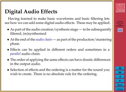
<strong>Digital</strong> <strong>Audio</strong> <strong>Effects</strong><br />
Having learned to make basic waveforms and basic filtering lets<br />
see how we can add some digital audio effects. These may be applied:<br />
• As part of the audio creation/synthesis stage — to be subsequently<br />
filtered, (re)synthesised<br />
• At the end of the audio chain — as part of the production/mastering<br />
phase.<br />
• <strong>Effects</strong> can be applied in different orders and sometimes in a<br />
parallel audio chain.<br />
• The order of applying the same effects can have drastic differences<br />
in the output audio.<br />
• Selection of effects and the ordering is a matter for the sound you<br />
wish to create. There is no absolute rule for the ordering.<br />
CM0268<br />
MATLAB<br />
DSP<br />
GRAPHICS<br />
332<br />
1<br />
◭◭<br />
◮◮<br />
◭<br />
◮<br />
Back<br />
Close
Effect Types and Parameters<br />
Typical Guitar (and other) <strong>Effects</strong> Pipeline<br />
Some Linking ordering <strong>Effects</strong> is standard for some audio processing, E.g:<br />
Compression → Distortion → EQ →modules Noise<br />
to on<br />
Redux<br />
or off.<br />
→ Amp Sim →<br />
The patches of the G1/G1X consist of eight<br />
Modulation → Delay → Reverb<br />
serially linked effect modules, as shown in the<br />
Common for some guitar effects pedal:<br />
Compressor<br />
Auto Wah<br />
Booster<br />
Tremolo<br />
Phaser<br />
FD Clean<br />
VX Clean<br />
HW Clean<br />
US Blues<br />
BG Crunch<br />
ZNR<br />
Effect modules<br />
illustration below. You can use all effect<br />
modules together or selectively set certain<br />
COMP/EFX DRIVE EQ ZNR AMP MODULATION DELAY REVERB<br />
AMP Sim.<br />
Chorus<br />
Ensemble<br />
Flanger<br />
Step<br />
Pitch Shift<br />
Delay<br />
Tape Echo<br />
Analog<br />
Delay<br />
Ping Pong<br />
Delay<br />
Hall<br />
Room<br />
Spring<br />
Arena<br />
Tiled Room<br />
CM0268<br />
MATLAB<br />
DSP<br />
GRAPHICS<br />
333<br />
Effect types<br />
* Manufacturer names and product names mentioned in this listing are trademarks or<br />
registered trademarks of their respective owners. The names are used only to illustrate sonic<br />
characteristics and do not indicate any affiliation with ZOOM CORPORATION.<br />
For some effect modules, you can select an effect type from several possible choices. For example, the<br />
MODULATION module comprises Chorus, Flanger, and other effect types. The REVERB module<br />
comprises Hall, Room, and other effect types from which you can choose one.<br />
Note: Other <strong>Effects</strong> Units allow for a completely reconfigurable<br />
effects pipeline. E.g. Boss GT-8<br />
● Tap<br />
1<br />
◭◭<br />
◮◮<br />
◭<br />
◮<br />
Back<br />
Close
Classifying <strong>Effects</strong><br />
<strong>Audio</strong> effects can be classified by the way do their processing:<br />
<strong>Basic</strong> Filtering — Lowpass, Highpass filter etc,, Equaliser<br />
Time Varying Filters — Wah-wah, Phaser<br />
Delays — Vibrato, Flanger, Chorus, Echo<br />
Modulators — Ring modulation, Tremolo, Vibrato<br />
Non-linear Processing — Compression, Limiters, Distortion,<br />
Exciters/Enhancers<br />
Spacial <strong>Effects</strong> — Panning, Reverb, Surround Sound<br />
CM0268<br />
MATLAB<br />
DSP<br />
GRAPHICS<br />
334<br />
1<br />
◭◭<br />
◮◮<br />
◭<br />
◮<br />
Back<br />
Close
<strong>Basic</strong> <strong>Digital</strong> <strong>Audio</strong> Filtering <strong>Effects</strong>:<br />
Equalisers<br />
Filters by definition remove/attenuate audio from the spectrum<br />
above or below some cut-off frequency.<br />
CM0268<br />
MATLAB<br />
DSP<br />
GRAPHICS<br />
335<br />
• For many audio applications this a little too restrictive<br />
Equalisers, by contrast, enhance/diminish certain frequency bands<br />
whilst leaving others unchanged:<br />
• Built using a series of shelving and peak filters<br />
• First or second-order filters usually employed.<br />
1<br />
◭◭<br />
◮◮<br />
◭<br />
◮<br />
Back<br />
Close
Shelving and Peak Filters<br />
Shelving Filter — Boost or cut the low or high frequency bands with<br />
a cut-off frequency, F c and gain G<br />
CM0268<br />
MATLAB<br />
DSP<br />
GRAPHICS<br />
336<br />
Peak Filter — Boost or cut mid-frequency bands with a cut-off<br />
frequency, F c , a bandwidth, f b and gain G<br />
1<br />
◭◭<br />
◮◮<br />
◭<br />
◮<br />
Back<br />
Close
Shelving Filters<br />
A first-order shelving filter may be described by the transfer function:<br />
H(z) = 1 + H 0<br />
(1 ± A(z)) where LF/HF + /−<br />
2<br />
where A(z) is a first-order allpass filter — passes all frequencies<br />
but modifies phase:<br />
CM0268<br />
MATLAB<br />
DSP<br />
GRAPHICS<br />
337<br />
A(z) = z−1 + a B/C<br />
1 + a B/C z −1 B=Boost, C=Cut<br />
which leads the following algorithm/difference equation:<br />
1<br />
y 1 (n) = a B/C x(n) + x(n − 1) − a B/C y 1 (n − 1)<br />
y(n) = H 0<br />
2 (x(n) ± y 1(n)) + x(n)<br />
◭◭<br />
◮◮<br />
◭<br />
◮<br />
Back<br />
Close
Shelving Filters (Cont.)<br />
The gain, G, in dB can be adjusted accordingly:<br />
H 0 = V 0 − 1 where V 0 = 10 G/20<br />
CM0268<br />
MATLAB<br />
DSP<br />
GRAPHICS<br />
338<br />
and the cut-off frequency for boost, a B , or cut, a C are given by:<br />
a B = tan(2πf c/f s ) − 1<br />
tan(2πf c /f s ) + 1<br />
a C = tan(2πf c/f s ) − V 0<br />
tan(2πf c /f s ) − V 0<br />
1<br />
◭◭<br />
◮◮<br />
◭<br />
◮<br />
Back<br />
Close
Shelving Filters Signal Flow Graph<br />
x(n)<br />
H 0 /2<br />
A(z) y 1 (n) ± ×<br />
+<br />
y(n)<br />
CM0268<br />
MATLAB<br />
DSP<br />
GRAPHICS<br />
339<br />
where A(z) is given by:<br />
x(n)<br />
T<br />
x(n − 1)<br />
×<br />
a B/C × 1<br />
+ +<br />
y(n)<br />
1<br />
× −a B/C<br />
y 1 (n − 1)<br />
T<br />
◭◭<br />
◮◮<br />
◭<br />
◮<br />
Back<br />
Close
Peak Filters<br />
A first-order shelving filter may be described by the transfer function:<br />
H(z) = 1 + H 0<br />
2 (1 − A 2(z))<br />
where A 2 (z) is a second-order allpass filter:<br />
CM0268<br />
MATLAB<br />
DSP<br />
GRAPHICS<br />
340<br />
A(z) = −a B + (d − da B )z −1 + z −2<br />
1 + (d − da B )z −1 + a B z −2<br />
which leads the following algorithm/difference equation:<br />
y 1 (n) = 1a B/C x(n) + d(1 − a B/C )x(n − 1) + x(n − 2)<br />
−d(1 − a B/C )y 1 (n − 1) + a B/C y 1 (n − 2)<br />
y(n) = H 0<br />
2 (x(n) − y 1(n)) + x(n)<br />
1<br />
◭◭<br />
◮◮<br />
◭<br />
◮<br />
Back<br />
Close
Peak Filters (Cont.)<br />
The center/cut-off frequency, d, is given by:<br />
d = −cos(2πf c /f s )<br />
The H 0 by relation to the gain, G, as before:<br />
H 0 = V 0 − 1 where V 0 = 10 G/20<br />
CM0268<br />
MATLAB<br />
DSP<br />
GRAPHICS<br />
341<br />
and the bandwidth, f b is given by the limits for boost, a B , or cut,<br />
a C are given by:<br />
1<br />
a B = tan(2πf b/f s ) − 1<br />
tan(2πf b /f s ) + 1<br />
a C = tan(2πf b/f s ) − V 0<br />
tan(2πf b /f s ) − V 0<br />
◭◭<br />
◮◮<br />
◭<br />
◮<br />
Back<br />
Close
Peak Filters Signal Flow Graph<br />
x(n)<br />
−1 H 0 /2<br />
× ×<br />
A(z) y 1 (n) +<br />
+<br />
y(n)<br />
CM0268<br />
MATLAB<br />
DSP<br />
GRAPHICS<br />
342<br />
where A(z) is given by:<br />
x(n)<br />
T<br />
x(n − 1) x(n − 2)<br />
T<br />
× −a B/C × d(1 − a B/C ) × 1<br />
+ + +<br />
y(n)<br />
1<br />
×<br />
a B/C × −d(1 − a B/C )<br />
T<br />
y 1 (n − 2) y 1 (n − 1)<br />
T<br />
◭◭<br />
◮◮<br />
◭<br />
◮<br />
Back<br />
Close
Shelving Filter EQ MATLAB Example<br />
The following function, shelving.m performs a shelving filter:<br />
function [b, a] = shelving(G, fc, fs, Q, type)<br />
%<br />
% Derive coefficients for a shelving filter with a given amplitude<br />
% and cutoff frequency. All coefficients are calculated as<br />
% described in Zolzer’s DAFX book (p. 50 -55).<br />
%<br />
% Usage: [B,A] = shelving(G, Fc, Fs, Q, type);<br />
%<br />
% G is the logrithmic gain (in dB)<br />
% FC is the center frequency<br />
% Fs is the sampling rate<br />
% Q adjusts the slope be replacing the sqrt(2) term<br />
% type is a character string defining filter type<br />
% Choices are: ’Base_Shelf’ or ’Treble_Shelf’<br />
%Error Check<br />
if((strcmp(type,’Base_Shelf’) ˜= 1) && ...<br />
(strcmp(type,’Treble_Shelf’) ˜= 1))<br />
error([’Unsupported Filter Type: ’ type]);<br />
end<br />
CM0268<br />
MATLAB<br />
DSP<br />
GRAPHICS<br />
343<br />
1<br />
◭◭<br />
◮◮<br />
◭<br />
◮<br />
Back<br />
Close
K = tan((pi * fc)/fs);<br />
V0 = 10ˆ(G/20);<br />
root2 = 1/Q; %sqrt(2)<br />
%Invert gain if a cut<br />
if(V0 < 1)<br />
V0 = 1/V0;<br />
end<br />
CM0268<br />
MATLAB<br />
DSP<br />
GRAPHICS<br />
344<br />
%%%%%%%%%%%%%%%%%%%%<br />
% BASE BOOST<br />
%%%%%%%%%%%%%%%%%%%%<br />
if(( G > 0 ) & (strcmp(type,’Base_Shelf’)))<br />
b0 = (1 + sqrt(V0)*root2*K + V0*Kˆ2) / (1 + root2*K + Kˆ2);<br />
b1 = (2 * (V0*Kˆ2 - 1) ) / (1 + root2*K + Kˆ2);<br />
b2 = (1 - sqrt(V0)*root2*K + V0*Kˆ2) / (1 + root2*K + Kˆ2);<br />
a1 = (2 * (Kˆ2 - 1) ) / (1 + root2*K + Kˆ2);<br />
a2 = (1 - root2*K + Kˆ2) / (1 + root2*K + Kˆ2);<br />
%%%%%%%%%%%%%%%%%%%%<br />
% BASE CUT<br />
%%%%%%%%%%%%%%%%%%%%<br />
elseif (( G < 0 ) & (strcmp(type,’Base_Shelf’)))<br />
b0 = (1 + root2*K + Kˆ2) / (1 + root2*sqrt(V0)*K + V0*Kˆ2);<br />
1<br />
◭◭<br />
◮◮<br />
◭<br />
◮<br />
Back<br />
Close
1 = (2 * (Kˆ2 - 1) ) / (1 + root2*sqrt(V0)*K + V0*Kˆ2);<br />
b2 = (1 - root2*K + Kˆ2) / (1 + root2*sqrt(V0)*K + V0*Kˆ2);<br />
a1 = (2 * (V0*Kˆ2 - 1) ) / (1 + root2*sqrt(V0)*K + V0*Kˆ2);<br />
a2 = (1 - root2*sqrt(V0)*K + V0*Kˆ2) / ...<br />
(1 + root2*sqrt(V0)*K + V0*Kˆ2);<br />
%%%%%%%%%%%%%%%%%%%%<br />
% TREBLE BOOST<br />
%%%%%%%%%%%%%%%%%%%%<br />
elseif (( G > 0 ) & (strcmp(type,’Treble_Shelf’)))<br />
CM0268<br />
MATLAB<br />
DSP<br />
GRAPHICS<br />
345<br />
b0 = (V0 + root2*sqrt(V0)*K + Kˆ2) / (1 + root2*K + Kˆ2);<br />
b1 = (2 * (Kˆ2 - V0) ) / (1 + root2*K + Kˆ2);<br />
b2 = (V0 - root2*sqrt(V0)*K + Kˆ2) / (1 + root2*K + Kˆ2);<br />
a1 = (2 * (Kˆ2 - 1) ) / (1 + root2*K + Kˆ2);<br />
a2 = (1 - root2*K + Kˆ2) / (1 + root2*K + Kˆ2);<br />
%%%%%%%%%%%%%%%%%%%%<br />
% TREBLE CUT<br />
%%%%%%%%%%%%%%%%%%%%<br />
elseif (( G < 0 ) & (strcmp(type,’Treble_Shelf’)))<br />
b0 = (1 + root2*K + Kˆ2) / (V0 + root2*sqrt(V0)*K + Kˆ2);<br />
b1 = (2 * (Kˆ2 - 1) ) / (V0 + root2*sqrt(V0)*K + Kˆ2);<br />
b2 = (1 - root2*K + Kˆ2) / (V0 + root2*sqrt(V0)*K + Kˆ2);<br />
a1 = (2 * ((Kˆ2)/V0 - 1) ) / (1 + root2/sqrt(V0)*K ...<br />
1<br />
◭◭<br />
◮◮<br />
◭<br />
◮<br />
Back<br />
Close
+ (Kˆ2)/V0);<br />
a2 = (1 - root2/sqrt(V0)*K + (Kˆ2)/V0) / ....<br />
(1 + root2/sqrt(V0)*K + (Kˆ2)/V0);<br />
%%%%%%%%%%%%%%%%%%%%<br />
% All-Pass<br />
%%%%%%%%%%%%%%%%%%%%<br />
else<br />
b0 = V0;<br />
b1 = 0;<br />
b2 = 0;<br />
a1 = 0;<br />
a2 = 0;<br />
end<br />
CM0268<br />
MATLAB<br />
DSP<br />
GRAPHICS<br />
346<br />
%return values<br />
a = [ 1, a1, a2];<br />
b = [ b0, b1, b2];<br />
1<br />
◭◭<br />
◮◮<br />
◭<br />
◮<br />
Back<br />
Close
Shelving Filter EQ MATLAB Example (Cont.)<br />
The following script shelving eg.m illustrates how we use the shelving<br />
filter function to filter:<br />
infile = ’acoustic.wav’;<br />
% read in wav sample<br />
[ x, Fs, N ] = wavread(infile);<br />
CM0268<br />
MATLAB<br />
DSP<br />
GRAPHICS<br />
347<br />
%set Parameters for Shelving Filter<br />
% Change these to experiment with filter<br />
G = 4; fcb = 300; Q = 3; type = ’Base_Shelf’;<br />
[b a] = shelving(G, fcb, Fs, Q, type);<br />
yb = filter(b,a, x);<br />
% write output wav files<br />
wavwrite(yb, Fs, N, ’out_bassshelf.wav’);<br />
% plot the original and equalised waveforms<br />
figure(1), hold on;<br />
plot(yb,’b’);<br />
plot(x,’r’);<br />
title(’Bass Shelf Filter Equalised Signal’);<br />
1<br />
◭◭<br />
◮◮<br />
◭<br />
◮<br />
Back<br />
Close
%Do treble shelf filter<br />
fct = 600; type = ’Treble_Shelf’;<br />
[b a] = shelving(G, fct, Fs, Q, type);<br />
yt = filter(b,a, x);<br />
% write output wav files<br />
wavwrite(yt, Fs, N, ’out_treblehelf.wav’);<br />
figure(1), hold on;<br />
plot(yb,’g’);<br />
plot(x,’r’);<br />
title(’Treble Shelf Filter Equalised Signal’);<br />
CM0268<br />
MATLAB<br />
DSP<br />
GRAPHICS<br />
348<br />
1<br />
◭◭<br />
◮◮<br />
◭<br />
◮<br />
Back<br />
Close
Shelving Filter EQ MATLAB Example (Cont.)<br />
The output from the above code is (red plot is original audio):<br />
1.5<br />
1<br />
0.5<br />
Bass Shelf Filter Equalised Signal<br />
1.5<br />
1<br />
0.5<br />
Treble Shelf Filter Equalised Signal<br />
CM0268<br />
MATLAB<br />
DSP<br />
GRAPHICS<br />
349<br />
0<br />
0<br />
−0.5<br />
−0.5<br />
−1<br />
−1<br />
−1.5<br />
0 5 10 15<br />
x 10 4<br />
−1.5<br />
0 5 10 15<br />
x 10 4<br />
1<br />
Click here to hear: original audio, bass shelf filtered audio,<br />
treble shelf filtered audio.<br />
◭◭<br />
◮◮<br />
◭<br />
◮<br />
Back<br />
Close
Time-varying Filters<br />
Some common effects are realised by simply time varying a filter<br />
in a couple of different ways:<br />
Wah-wah — A bandpass filter with a time varying centre (resonant)<br />
frequency and a small bandwidth. Filtered signal mixed with<br />
direct signal.<br />
Phasing — A notch filter, that can be realised as set of cascading IIR<br />
filters, again mixed with direct signal.<br />
CM0268<br />
MATLAB<br />
DSP<br />
GRAPHICS<br />
350<br />
1<br />
◭◭<br />
◮◮<br />
◭<br />
◮<br />
Back<br />
Close
Wah-wah Example<br />
The signal flow for a wah-wah is as follows:<br />
x(n)<br />
Time<br />
Varying<br />
BP<br />
direct-mix<br />
×<br />
wah-mix<br />
where BP is a time varying frequency bandpass filter.<br />
• A phaser is similarly implemented with a notch filter replacing<br />
the bandpass filter.<br />
• A variation is the M-fold wah-wah filter where M tap delay<br />
bandpass filters spread over the entire spectrum change their<br />
centre frequencies simultaneously.<br />
• A bell effect can be achieved with around a hundred M tap<br />
delays and narrow bandwidth filters<br />
×<br />
+<br />
y(n)<br />
CM0268<br />
MATLAB<br />
DSP<br />
GRAPHICS<br />
351<br />
1<br />
◭◭<br />
◮◮<br />
◭<br />
◮<br />
Back<br />
Close
Time Varying Filter Implementation:<br />
State Variable Filter<br />
In our audio application of time varying filters we now want<br />
independent control over the cut-off frequency and damping factor<br />
of a filter.<br />
CM0268<br />
MATLAB<br />
DSP<br />
GRAPHICS<br />
352<br />
(Borrowed from analog electronics) we can implement a<br />
State Variable Filter to solve this problem.<br />
• One further advantage is that we can simultaneously get lowpass,<br />
bandpass and highpass filter output.<br />
1<br />
◭◭<br />
◮◮<br />
◭<br />
◮<br />
Back<br />
Close
The State Variable Filter<br />
x(n)<br />
+ +<br />
y h (n)<br />
F 1<br />
× +<br />
y b (n)<br />
F 1<br />
× +<br />
y l (n)<br />
CM0268<br />
MATLAB<br />
DSP<br />
GRAPHICS<br />
353<br />
T<br />
T<br />
−1 × Q 1<br />
×<br />
T<br />
where:<br />
−1<br />
×<br />
T<br />
x(n) = input signal<br />
y l (n) = lowpass signal<br />
y b (n) = bandpass signal<br />
y h (n) = highpass signal<br />
1<br />
◭◭<br />
◮◮<br />
◭<br />
◮<br />
Back<br />
Close
The State Variable Filter Algorithm<br />
The algorithm difference equations are given by:<br />
y l (n) = F 1 y b (n) + y l (n − 1)<br />
y b (n) = F 1 y h (n) + y b (n − 1)<br />
y h (n) = x(n) − y l (n − 1) − Q 1 y b (n − 1)<br />
CM0268<br />
MATLAB<br />
DSP<br />
GRAPHICS<br />
354<br />
with tuning coefficients F 1 and Q 1 related to the cut-off frequency,<br />
f c , and damping, d:<br />
F 1 = 2 sin(πf c /f s ),<br />
and Q 1 = 2d<br />
1<br />
◭◭<br />
◮◮<br />
◭<br />
◮<br />
Back<br />
Close
MATLAB Wah-wah Implementation<br />
We simply implement the State Variable Filter with a variable<br />
frequency, f c . The code listing is wah wah.m:<br />
% wah_wah.m state variable band pass<br />
%<br />
% BP filter with narrow pass band, Fc oscillates up and<br />
% down the spectrum<br />
% Difference equation taken from DAFX chapter 2<br />
%<br />
CM0268<br />
MATLAB<br />
DSP<br />
GRAPHICS<br />
% Changing this from a BP to a BR/BS (notch instead of a bandpass) converts<br />
% this effect to a phaser<br />
%<br />
% yl(n) = F1*yb(n) + yl(n-1)<br />
% yb(n) = F1*yh(n) + yb(n-1)<br />
% yh(n) = x(n) - yl(n-1) - Q1*yb(n-1)<br />
%<br />
% vary Fc from 500 to 5000 Hz<br />
infile = ’acoustic.wav’;<br />
% read in wav sample<br />
[ x, Fs, N ] = wavread(infile);<br />
355<br />
1<br />
◭◭<br />
◮◮<br />
◭<br />
◮<br />
Back<br />
Close
%%%%%%% EFFECT COEFFICIENTS %%%%%%%%%%%%%%%%%%%%%%%%%%%%%<br />
%%%%%%%%%%%%%%%%%%%%%%%%%%%%%%%%%%%%%%%%%%%%%%%%%<br />
% damping factor<br />
% lower the damping factor the smaller the pass band<br />
damp = 0.05;<br />
% min and max centre cutoff frequency of variable bandpass filter<br />
minf=500;<br />
maxf=3000;<br />
CM0268<br />
MATLAB<br />
DSP<br />
GRAPHICS<br />
356<br />
% wah frequency, how many Hz per second are cycled through<br />
Fw = 2000;<br />
%%%%%%%%%%%%%%%%%%%%%%%%%%%%%%%%%%%%%%%%%%%%%%%%%<br />
% change in centre frequency per sample (Hz)<br />
delta = Fw/Fs;<br />
% create triangle wave of centre frequency values<br />
Fc=minf:delta:maxf;<br />
while(length(Fc) < length(x) )<br />
Fc= [ Fc (maxf:-delta:minf) ];<br />
Fc= [ Fc (minf:delta:maxf) ];<br />
end<br />
% trim tri wave to size of input<br />
Fc = Fc(1:length(x));<br />
1<br />
◭◭<br />
◮◮<br />
◭<br />
◮<br />
Back<br />
Close
% difference equation coefficients<br />
% must be recalculated each time Fc changes<br />
F1 = 2*sin((pi*Fc(1))/Fs);<br />
% this dictates size of the pass bands<br />
Q1 = 2*damp;<br />
yh=zeros(size(x));<br />
yb=zeros(size(x));<br />
yl=zeros(size(x));<br />
% create emptly out vectors<br />
CM0268<br />
MATLAB<br />
DSP<br />
GRAPHICS<br />
357<br />
% first sample, to avoid referencing of negative signals<br />
yh(1) = x(1);<br />
yb(1) = F1*yh(1);<br />
yl(1) = F1*yb(1);<br />
% apply difference equation to the sample<br />
for n=2:length(x),<br />
yh(n) = x(n) - yl(n-1) - Q1*yb(n-1);<br />
yb(n) = F1*yh(n) + yb(n-1);<br />
yl(n) = F1*yb(n) + yl(n-1);<br />
F1 = 2*sin((pi*Fc(n))/Fs);<br />
end<br />
%normalise<br />
maxyb = max(abs(yb));<br />
yb = yb/maxyb;<br />
1<br />
◭◭<br />
◮◮<br />
◭<br />
◮<br />
Back<br />
Close
% write output wav files<br />
wavwrite(yb, Fs, N, ’out_wah.wav’);<br />
figure(1)<br />
hold on<br />
plot(x,’r’);<br />
plot(yb,’b’);<br />
title(’Wah-wah and original Signal’);<br />
CM0268<br />
MATLAB<br />
DSP<br />
GRAPHICS<br />
358<br />
1<br />
◭◭<br />
◮◮<br />
◭<br />
◮<br />
Back<br />
Close
Wah-wah MATLAB Example (Cont.)<br />
The output from the above code is (red plot is original audio):<br />
1<br />
0.8<br />
0.6<br />
0.4<br />
Wah−wah and original Signal<br />
CM0268<br />
MATLAB<br />
DSP<br />
GRAPHICS<br />
359<br />
0.2<br />
0<br />
−0.2<br />
−0.4<br />
−0.6<br />
−0.8<br />
−1<br />
0 5 10 15<br />
x 10 4<br />
1<br />
Click here to hear: original audio, wah-wah filtered audio.<br />
◭◭<br />
◮◮<br />
◭<br />
◮<br />
Back<br />
Close
Wah-wah Code Explained<br />
Three main parts:<br />
• Create a triangle wave to modulate the centre frequency of the<br />
bandpass filter.<br />
• Implementation of state variable filter<br />
• Repeated recalculation if centre frequency within the state variable<br />
filter loop.<br />
CM0268<br />
MATLAB<br />
DSP<br />
GRAPHICS<br />
360<br />
1<br />
◭◭<br />
◮◮<br />
◭<br />
◮<br />
Back<br />
Close
Wah-wah Code Explained (Cont.)<br />
Creation of triangle waveform we have seen previously— see<br />
waveforms.m.<br />
• Slight modification of this code here to allow ’frequency values’<br />
(Y-axis amplitude) to vary rather than frequency of the triangle<br />
waveform — here the frequency of the modulator wave is<br />
determined by wah-wah rate, F w, usually a low frequency:<br />
% min and max centre cutoff frequency of variable bandpass filter<br />
minf=500; maxf=3000;<br />
% wah frequency, how many Hz per second are cycled through<br />
Fw = 2000;<br />
CM0268<br />
MATLAB<br />
DSP<br />
GRAPHICS<br />
361<br />
% change in centre frequency per sample (Hz)<br />
delta = Fw/Fs;<br />
% create triangle wave of centre frequency values<br />
Fc=minf:delta:maxf;<br />
while(length(Fc) < length(x) )<br />
Fc= [ Fc (maxf:-delta:minf) ];<br />
Fc= [ Fc (minf:delta:maxf) ];<br />
end<br />
% trim tri wave to size of input<br />
Fc = Fc(1:length(x));<br />
1<br />
◭◭<br />
◮◮<br />
◭<br />
◮<br />
Back<br />
Close
Wah-wah Code Explained (Cont.)<br />
Note: As the Wah-wah rate is not likely to be in perfect sync with<br />
input waveform, x, we must trim it to the same length as x.<br />
Modifications to Wah-wah<br />
• Adding Multiple Delays with differing centre frequency filters<br />
but all modulated by same Fc gives an M-fold wah-wah<br />
• Changing filter to a notch filter gives a phaser<br />
– Notch Filter (or bandreject/bandstop filter (BR/BS)) —<br />
attenuate frequencies in a narrow bandwidth (High Q factor)<br />
around cut-off frequency, u 0<br />
• See Lab worksheet and useful for coursework<br />
CM0268<br />
MATLAB<br />
DSP<br />
GRAPHICS<br />
362<br />
1<br />
◭◭<br />
◮◮<br />
◭<br />
◮<br />
Back<br />
Close
Bandreject (BR)/Bandpass(BP) Filters<br />
(Sort of) Seen before (Peak Filter). Here we have, BR/BP:<br />
x(n)<br />
BR = +<br />
BP = −<br />
A 2 (z) y 1 (n) ±<br />
1/2<br />
×<br />
y(n)<br />
CM0268<br />
MATLAB<br />
DSP<br />
GRAPHICS<br />
363<br />
where A 2 (z) (a second order allpass filter) is given by:<br />
x(n)<br />
T<br />
x(n − 1) x(n − 2)<br />
T<br />
× −c × d(1 − c) × 1<br />
1<br />
+ + +<br />
× c × −d(1 − c)<br />
T<br />
y 1 (n − 2) y 1 (n − 1)<br />
T<br />
y(n)<br />
◭◭<br />
◮◮<br />
◭<br />
◮<br />
Back<br />
Close
Bandreject (BR)/Bandpass(BP) Filters (Cont.)<br />
The difference equation is given by:<br />
y 1 (n) = −cx(n) + d(1 − c)x(n − 1) + x(n − 2)<br />
−d(1 − c)y 1 (n − 1) + cy 1 (n − 2)<br />
y(n) = 1 2 (x(n) ± y 1(n))<br />
CM0268<br />
MATLAB<br />
DSP<br />
GRAPHICS<br />
364<br />
where<br />
d = −cos(2πf c /f s )<br />
Bandreject = +<br />
Bandpass = −<br />
c = tan(2πf c/f s ) − 1<br />
tan(2πf c /f s ) + 1<br />
1<br />
◭◭<br />
◮◮<br />
◭<br />
◮<br />
Back<br />
Close
Delay Based <strong>Effects</strong><br />
Many useful audio effects can be implemented using a delay<br />
structure:<br />
• Sounds reflected of walls<br />
– In a cave or large room we here an echo and also reverberation<br />
takes place – this is a different effect — see later<br />
– If walls are closer together repeated reflections can appear<br />
as parallel boundaries and we hear a modification of sound<br />
colour instead.<br />
• Vibrato, Flanging, Chorus and Echo are examples of delay effects<br />
CM0268<br />
MATLAB<br />
DSP<br />
GRAPHICS<br />
365<br />
1<br />
◭◭<br />
◮◮<br />
◭<br />
◮<br />
Back<br />
Close
<strong>Basic</strong> Delay Structure<br />
We build basic delay structures out of some very basic FIR and IIR<br />
filters:<br />
• We use FIR and IIR comb filters<br />
• Combination of FIR and IIR gives the Universal Comb Filter<br />
CM0268<br />
MATLAB<br />
DSP<br />
GRAPHICS<br />
366<br />
1<br />
◭◭<br />
◮◮<br />
◭<br />
◮<br />
Back<br />
Close
FIR Comb Filter<br />
This simulates a single delay:<br />
• The input signal is delayed by a given time duration, τ.<br />
• The delayed (processed) signal is added to the input signal some<br />
amplitude gain, g<br />
• The difference equation is simply:<br />
CM0268<br />
MATLAB<br />
DSP<br />
GRAPHICS<br />
367<br />
y(n) = x(n) + gx(n − M)<br />
with M = τ/f s<br />
• The transfer function is:<br />
H(z) = 1 + gz −M<br />
1<br />
◭◭<br />
◮◮<br />
◭<br />
◮<br />
Back<br />
Close
FIR Comb Filter Signal Flow Diagram<br />
x(n)<br />
×<br />
1<br />
T M<br />
+ y(n)<br />
CM0268<br />
MATLAB<br />
DSP<br />
GRAPHICS<br />
368<br />
x(n − M)<br />
×<br />
1<br />
g<br />
◭◭<br />
◮◮<br />
◭<br />
◮<br />
Back<br />
Close
FIR Comb Filter MATLAB Code<br />
fircomb.m:<br />
CM0268<br />
MATLAB<br />
DSP<br />
GRAPHICS<br />
369<br />
x=zeros(100,1);x(1)=1; % unit impulse signal of length 100<br />
g=0.5; %Example gain<br />
Delayline=zeros(10,1); % memory allocation for length 10<br />
for n=1:length(x);<br />
y(n)=x(n)+g*Delayline(10);<br />
Delayline=[x(n);Delayline(1:10-1)];<br />
end;<br />
1<br />
◭◭<br />
◮◮<br />
◭<br />
◮<br />
Back<br />
Close
IIR Comb Filter<br />
This simulates a single delay:<br />
• Simulates endless reflections at both ends of cylinder.<br />
• We get an endless series of responses, y(n) to input, x(n).<br />
• The input signal circulates in delay line (delay time τ) that is fed<br />
back to the input..<br />
• Each time it is fed back it is attenuated by g.<br />
• Input sometime scaled by c to compensate for high amplification<br />
of the structure.<br />
• The difference equation is simply:<br />
y(n) = Cx(n) + gy(n − M)<br />
• The transfer function is:<br />
c<br />
H(z) =<br />
1 − gz −M<br />
with M = τ/f s<br />
CM0268<br />
MATLAB<br />
DSP<br />
GRAPHICS<br />
370<br />
1<br />
◭◭<br />
◮◮<br />
◭<br />
◮<br />
Back<br />
Close
IIR Comb Filter Signal Flow Diagram<br />
x(n)<br />
× +<br />
y(n)<br />
CM0268<br />
MATLAB<br />
DSP<br />
GRAPHICS<br />
371<br />
c<br />
T M<br />
× y(n − M)<br />
1<br />
g<br />
◭◭<br />
◮◮<br />
◭<br />
◮<br />
Back<br />
Close
IIR Comb Filter MATLAB Code<br />
iircomb.m:<br />
CM0268<br />
MATLAB<br />
DSP<br />
GRAPHICS<br />
372<br />
x=zeros(100,1);x(1)=1; % unit impulse signal of length 100<br />
g=0.5;<br />
Delayline=zeros(10,1); % memory allocation for length 10<br />
for n=1:length(x);<br />
y(n)=x(n)+g*Delayline(10);<br />
Delayline=[y(n);Delayline(1:10-1)];<br />
end;<br />
1<br />
◭◭<br />
◮◮<br />
◭<br />
◮<br />
Back<br />
Close
Universal Comb Filter<br />
The combination of the FIR and IIR comb filters yields the Universal<br />
Comb Filter:<br />
• <strong>Basic</strong>ally this is an allpass filter with an M sample delay operator<br />
and an additional multiplier, FF.<br />
BL<br />
×<br />
CM0268<br />
MATLAB<br />
DSP<br />
GRAPHICS<br />
373<br />
x(n)<br />
FF<br />
x(n − M)<br />
T M<br />
+ × +<br />
y(n)<br />
1<br />
FB<br />
×<br />
• Parameters: FF = feedforward, FB = feedbackward, BL = blend<br />
◭◭<br />
◮◮<br />
◭<br />
◮<br />
Back<br />
Close
Universal Comb Filter Parameters<br />
CM0268<br />
MATLAB<br />
DSP<br />
GRAPHICS<br />
Universal in that we can form any comb filter, an allpass or a delay:<br />
374<br />
BL FB FF<br />
FIR Comb 1 0 g<br />
IIR Comb 1 g 0<br />
Allpass a −a 1<br />
delay 0 0 1<br />
1<br />
◭◭<br />
◮◮<br />
◭<br />
◮<br />
Back<br />
Close
Universal Comb Filter MATLAB Code<br />
unicomb.m:<br />
x=zeros(100,1);x(1)=1; % unit impulse signal of length 100<br />
CM0268<br />
MATLAB<br />
DSP<br />
GRAPHICS<br />
375<br />
BL=0.5;<br />
FB=-0.5;<br />
FF=1;<br />
M=10;<br />
Delayline=zeros(M,1); % memory allocation for length 10<br />
for n=1:length(x);<br />
xh=x(n)+FB*Delayline(M);<br />
y(n)=FF*Delayline(M)+BL*xh;<br />
Delayline=[xh;Delayline(1:M-1)];<br />
end;<br />
1<br />
◭◭<br />
◮◮<br />
◭<br />
◮<br />
Back<br />
Close
Vibrato - A Simple Delay Based Effect<br />
• Vibrato — Varying the time delay periodically<br />
• If we vary the distance between and observer and a sound source<br />
(cf. Doppler effect) we here a change in pitch.<br />
• Implementation: A Delay line and a low frequency oscillator (LFO)<br />
to vary the delay.<br />
• Only listen to the delay — no forward or backward feed.<br />
• Typical delay time = 5–10 Ms and LFO rate 5–14Hz.<br />
CM0268<br />
MATLAB<br />
DSP<br />
GRAPHICS<br />
376<br />
1<br />
◭◭<br />
◮◮<br />
◭<br />
◮<br />
Back<br />
Close
Vibrato MATLAB Code<br />
vibrato.m function, Use vibrato eg.m to call function:<br />
function y=vibrato(x,SAMPLERATE,Modfreq,Width)<br />
ya_alt=0;<br />
Delay=Width; % basic delay of input sample in sec<br />
DELAY=round(Delay*SAMPLERATE); % basic delay in # samples<br />
WIDTH=round(Width*SAMPLERATE); % modulation width in # samples<br />
if WIDTH>DELAY<br />
error(’delay greater than basic delay !!!’);<br />
return;<br />
end;<br />
CM0268<br />
MATLAB<br />
DSP<br />
GRAPHICS<br />
377<br />
MODFREQ=Modfreq/SAMPLERATE; % modulation frequency in # samples<br />
LEN=length(x); % # of samples in WAV-file<br />
L=2+DELAY+WIDTH*2; % length of the entire delay<br />
Delayline=zeros(L,1); % memory allocation for delay<br />
y=zeros(size(x)); % memory allocation for output vector<br />
1<br />
◭◭<br />
◮◮<br />
◭<br />
◮<br />
Back<br />
Close
for n=1:(LEN-1)<br />
M=MODFREQ;<br />
MOD=sin(M*2*pi*n);<br />
ZEIGER=1+DELAY+WIDTH*MOD;<br />
i=floor(ZEIGER);<br />
frac=ZEIGER-i;<br />
Delayline=[x(n);Delayline(1:L-1)];<br />
%---Linear Interpolation-----------------------------<br />
y(n,1)=Delayline(i+1)*frac+Delayline(i)*(1-frac);<br />
%---Allpass Interpolation------------------------------<br />
%y(n,1)=(Delayline(i+1)+(1-frac)*Delayline(i)-(1-frac)*ya_alt);<br />
%ya_alt=ya(n,1);<br />
end<br />
CM0268<br />
MATLAB<br />
DSP<br />
GRAPHICS<br />
378<br />
1<br />
◭◭<br />
◮◮<br />
◭<br />
◮<br />
Back<br />
Close
Vibrato MATLAB Example (Cont.)<br />
The output from the above code is (red plot is original audio):<br />
0.3<br />
0.2<br />
0.1<br />
Vibrato First 500 Samples<br />
CM0268<br />
MATLAB<br />
DSP<br />
GRAPHICS<br />
379<br />
0<br />
−0.1<br />
−0.2<br />
−0.3<br />
−0.4<br />
0 50 100 150 200 250 300 350 400 450 500<br />
1<br />
Click here to hear: original audio, vibrato audio.<br />
◭◭<br />
◮◮<br />
◭<br />
◮<br />
Back<br />
Close
Vibrato MATLAB Code Explained<br />
Click here to hear: original audio, vibrato audio.<br />
The code should be relatively self explanatory, except for one part:<br />
• We work out the delay (modulated by a sinusoid) at each step, n:<br />
M=MODFREQ;<br />
MOD=sin(M*2*pi*n);<br />
ZEIGER=1+DELAY+WIDTH*MOD;<br />
CM0268<br />
MATLAB<br />
DSP<br />
GRAPHICS<br />
380<br />
• We then work out the nearest sample step: i=floor(ZEIGER);<br />
• The problem is that we have a fractional delay line value: ZEIGER<br />
ZEIGER = 11.2779<br />
i = 11<br />
1<br />
ZEIGER = 11.9339<br />
i = 11<br />
ZEIGER = 12.2829<br />
i = 12<br />
◭◭<br />
◮◮<br />
◭<br />
◮<br />
Back<br />
Close
Fractional Delay Line - Interpolation<br />
• To improve effect we can use some form of interpolation to<br />
compute the output, y(n).<br />
– Above uses Linear Interpolation<br />
or:<br />
y(n,1)=Delayline(i+1)*frac+Delayline(i)*(1-frac);<br />
CM0268<br />
MATLAB<br />
DSP<br />
GRAPHICS<br />
381<br />
y(n) = x(n − (M + 1)).frac + x(n − M).(1 − frac)<br />
– Alternatives (commented in code)<br />
%---Allpass Interpolation------------------------------<br />
%y(n,1)=(Delayline(i+1)+(1-frac)*Delayline(i)-...<br />
(1-frac)*ya_alt);<br />
%ya_alt=y(n,1);<br />
1<br />
or:<br />
y(n) = x(n − (M + 1)).frac + x(n − M).(1 − frac) −<br />
y(n − 1).(1 − frac)<br />
– or spline based interpolation — see DAFX book p68-69.<br />
◭◭<br />
◮◮<br />
◭<br />
◮<br />
Back<br />
Close
Comb Filter Delay <strong>Effects</strong>:<br />
Flanger, Chorus, Slapback, Echo<br />
• A few popular effects can be made with a comb filter (FIR or IIR)<br />
and some modulation<br />
• Flanger, Chorus, Slapback, Echo same basic approach but different<br />
sound outputs:<br />
Effect Delay Range (ms) Modulation<br />
Resonator 0 . . . 20 None<br />
Flanger 0 . . . 15 Sinusoidal (≈ 1 Hz)<br />
Chorus 10 . . . 25 Random<br />
Slapback 25 . . . 50 None<br />
Echo > 50 None<br />
• Slapback (or doubling) — quick repetition of the sound,<br />
Flanging — continuously varying LFO of delay,<br />
Chorus — multiple copies of sound delayed by small random<br />
delays<br />
CM0268<br />
MATLAB<br />
DSP<br />
GRAPHICS<br />
382<br />
1<br />
◭◭<br />
◮◮<br />
◭<br />
◮<br />
Back<br />
Close
Flanger MATLAB Code<br />
flanger.m:<br />
% Creates a single FIR delay with the delay time oscillating from<br />
% Either 0-3 ms or 0-15 ms at 0.1 - 5 Hz<br />
infile=’acoustic.wav’;<br />
outfile=’out_flanger.wav’;<br />
CM0268<br />
MATLAB<br />
DSP<br />
GRAPHICS<br />
383<br />
% read the sample waveform<br />
[x,Fs,bits] = wavread(infile);<br />
% parameters to vary the effect %<br />
max_time_delay=0.003; % 3ms max delay in seconds<br />
rate=1; %rate of flange in Hz<br />
index=1:length(x);<br />
1<br />
% sin reference to create oscillating delay<br />
sin_ref = (sin(2*pi*index*(rate/Fs)))’;<br />
%convert delay in ms to max delay in samples<br />
max_samp_delay=round(max_time_delay*Fs);<br />
% create empty out vector<br />
y = zeros(length(x),1);<br />
◭◭<br />
◮◮<br />
◭<br />
◮<br />
Back<br />
Close
% to avoid referencing of negative samples<br />
y(1:max_samp_delay)=x(1:max_samp_delay);<br />
% set amp suggested coefficient from page 71 DAFX<br />
amp=0.7;<br />
% for each sample<br />
for i = (max_samp_delay+1):length(x),<br />
cur_sin=abs(sin_ref(i)); %abs of current sin val 0-1<br />
% generate delay from 1-max_samp_delay and ensure whole number<br />
cur_delay=ceil(cur_sin*max_samp_delay);<br />
% add delayed sample<br />
y(i) = (amp*x(i)) + amp*(x(i-cur_delay));<br />
end<br />
CM0268<br />
MATLAB<br />
DSP<br />
GRAPHICS<br />
384<br />
% write output<br />
wavwrite(y,Fs,outfile);<br />
1<br />
◭◭<br />
◮◮<br />
◭<br />
◮<br />
Back<br />
Close
Flanger MATLAB Example (Cont.)<br />
The output from the above code is (red plot is original audio):<br />
1.5<br />
1<br />
0.5<br />
Flanger and original Signal<br />
CM0268<br />
MATLAB<br />
DSP<br />
GRAPHICS<br />
385<br />
0<br />
−0.5<br />
−1<br />
−1.5<br />
0 5 10 15<br />
x 10 4<br />
1<br />
Click here to hear: original audio, flanged audio.<br />
◭◭<br />
◮◮<br />
◭<br />
◮<br />
Back<br />
Close
Modulation<br />
Modulation is the process where parameters of a sinusoidal signal<br />
(amplitude, frequency and phase) are modified or varied by an audio<br />
signal.<br />
We have met some example effects that could be considered as a<br />
class of modulation already:<br />
CM0268<br />
MATLAB<br />
DSP<br />
GRAPHICS<br />
386<br />
Amplitude Modulation — Wah-wah, Phaser<br />
Phase Modulation — Vibrato, Chorus, Flanger<br />
We will now introduce some Modulation effects.<br />
1<br />
◭◭<br />
◮◮<br />
◭<br />
◮<br />
Back<br />
Close
Ring Modulation<br />
Ring modulation (RM) is where the audio modulator signal, x(n)<br />
is multiplied by a sine wave, m(n), with a carrier frequency, f c .<br />
• This is very simple to implement digitally:<br />
y(n) = x(n).m(n)<br />
CM0268<br />
MATLAB<br />
DSP<br />
GRAPHICS<br />
387<br />
• Although audible result is easy to comprehend for simple signals<br />
things get more complicated for signals having numerous partials<br />
• If the modulator is also a sine wave with frequency, f x then one<br />
hears the sum and difference frequencies: f c + f x and f c − f x , for<br />
example.<br />
• When the input is periodic with at a fundamental frequency, f 0 ,<br />
then a spectrum with amplitude lines at frequencies |kf 0 ± f c |<br />
• Used to create robotic speech effects on old sci-fi movies and can<br />
create some odd almost non-musical effects if not used with care.<br />
(Original speech )<br />
1<br />
◭◭<br />
◮◮<br />
◭<br />
◮<br />
Back<br />
Close
MATLAB Ring Modulation<br />
Two examples, a sine wave and an audio sample being modulated<br />
by a sine wave, ring mod.m<br />
filename=’acoustic.wav’;<br />
% read the sample waveform<br />
[x,Fs,bits] = wavread(filename);<br />
CM0268<br />
MATLAB<br />
DSP<br />
GRAPHICS<br />
388<br />
index = 1:length(x);<br />
% Ring Modulate with a sine wave frequency Fc<br />
Fc = 440;<br />
carrier= sin(2*pi*index*(Fc/Fs))’;<br />
% Do Ring Modulation<br />
y = x.*carrier;<br />
% write output<br />
wavwrite(y,Fs,bits,’out_ringmod.wav’);<br />
Click here to hear: original audio, ring modulated audio.<br />
1<br />
◭◭<br />
◮◮<br />
◭<br />
◮<br />
Back<br />
Close
MATLAB Ring Modulation: Two sine waves<br />
% Ring Modulate with a sine wave frequency Fc<br />
Fc = 440;<br />
carrier= sin(2*pi*index*(Fc/Fs))’;<br />
%create a modulator sine wave frequency Fx<br />
Fx = 200;<br />
modulator = sin(2*pi*index*(Fx/Fs))’;<br />
CM0268<br />
MATLAB<br />
DSP<br />
GRAPHICS<br />
389<br />
% Ring Modulate with sine wave, freq. Fc<br />
y = modulator.*carrier;<br />
% write output<br />
wavwrite(y,Fs,bits,’twosine_ringmod.wav’);<br />
Output of Two sine wave ring modulation (f c = 440, f x = 380)<br />
1<br />
0.8<br />
1<br />
0.6<br />
0.4<br />
0.2<br />
0<br />
−0.2<br />
−0.4<br />
−0.6<br />
−0.8<br />
−1<br />
0 50 100 150 200 250<br />
Click here to hear: Two RM sine waves (f c = 440, f x = 200)<br />
◭◭<br />
◮◮<br />
◭<br />
◮<br />
Back<br />
Close
Amplitude Modulation<br />
Amplitude Modulation (AM) is defined by:<br />
y(n) = (1 + αm(n)).x(n)<br />
• Normalise the peak amplitude of M(n) to 1.<br />
• α is depth of modulation<br />
α = 1 gives maximum modulation<br />
α = 0 tuns off modulation<br />
• x(n) is the audio carrier signal<br />
• m(n) is a low-frequency oscillator modulator.<br />
• When x(n) and m(n) both sine waves with frequencies f c and<br />
f x respectively we here three frequencies: carrier, difference and<br />
sum: f c , f c − f x , f c + f x .<br />
CM0268<br />
MATLAB<br />
DSP<br />
GRAPHICS<br />
390<br />
1<br />
◭◭<br />
◮◮<br />
◭<br />
◮<br />
Back<br />
Close
Amplitude Modulation: Tremolo<br />
A common audio application of AM is to produce a tremolo effect:<br />
• Set modulation frequency of the sine wave to below 20Hz<br />
The MATLAB code to achieve this is tremolo1.m<br />
CM0268<br />
MATLAB<br />
DSP<br />
GRAPHICS<br />
391<br />
% read the sample waveform<br />
filename=’acoustic.wav’;<br />
[x,Fs,bits] = wavread(filename);<br />
index = 1:length(x);<br />
Fc = 5;<br />
alpha = 0.5;<br />
1<br />
trem=(1+ alpha*sin(2*pi*index*(Fc/Fs)))’;<br />
y = trem.*x;<br />
% write output<br />
wavwrite(y,Fs,bits,’out_tremolo1.wav’);<br />
Click here to hear: original audio, AM tremolo audio.<br />
◭◭<br />
◮◮<br />
◭<br />
◮<br />
Back<br />
Close
Tremolo via Ring Modulation<br />
If you ring modulate with a triangular wave (or try another waveform)<br />
you can get tremolo via RM, tremolo2.m<br />
% read the sample waveform<br />
filename=’acoustic.wav’;<br />
[x,Fs,bits] = wavread(filename);<br />
% create triangular wave LFO<br />
delta=5e-4;<br />
minf=-0.5;<br />
maxf=0.5;<br />
CM0268<br />
MATLAB<br />
DSP<br />
GRAPHICS<br />
392<br />
trem=minf:delta:maxf;<br />
while(length(trem) < length(x) )<br />
trem=[trem (maxf:-delta:minf)];<br />
trem=[trem (minf:delta:maxf)];<br />
end<br />
%trim trem<br />
trem = trem(1:length(x))’;<br />
1<br />
%Ring mod with triangular, trem<br />
y= x.*trem;<br />
% write output<br />
wavwrite(y,Fs,bits,’out_tremolo2.wav’);<br />
Click here to hear: original audio, RM tremolo audio.<br />
◭◭<br />
◮◮<br />
◭<br />
◮<br />
Back<br />
Close
Non-linear Processing<br />
Non-linear Processors are characterised by the fact that they create<br />
(intentional or unintentional) harmonic and inharmonic frequency<br />
components not present in the original signal.<br />
CM0268<br />
MATLAB<br />
DSP<br />
GRAPHICS<br />
393<br />
Three major categories of non-linear processing:<br />
Dynamic Processing: control of signal envelop — aim to minimise<br />
harmonic distortion Examples: Compressors, Limiters<br />
Intentional non-linear harmonic processing: Aim to introduce<br />
strong harmonic distortion. Examples: Many electric guitar effects<br />
such as distortion<br />
Exciters/Enhancers: add additional harmonics for subtle sound<br />
improvement.<br />
1<br />
◭◭<br />
◮◮<br />
◭<br />
◮<br />
Back<br />
Close
Limiter<br />
A Limiter is a device that controls high peaks in a signal but aims<br />
to change the dynamics of the main signal as little as possible:<br />
• A limiter makes use of a peak level measurement and aims to<br />
react very quickly to scale the level if it is above some threshold.<br />
• By lowering peaks the overall signal can be boosted.<br />
• Limiting used not only on single instrument but on final<br />
(multichannel) audio for CD mastering, radio broadcast etc.<br />
CM0268<br />
MATLAB<br />
DSP<br />
GRAPHICS<br />
394<br />
1<br />
◭◭<br />
◮◮<br />
◭<br />
◮<br />
Back<br />
Close
MATLAB Limiter Example<br />
The following code creates a modulated sine wave and then limits<br />
the amplitude when it exceeds some threshold,The MATLAB code<br />
to achieve this is limiter.m:<br />
%Create a sine wave with amplitude<br />
% reduced for half its duration<br />
CM0268<br />
MATLAB<br />
DSP<br />
GRAPHICS<br />
395<br />
anzahl=220;<br />
for n=1:anzahl,<br />
x(n)=0.2*sin(n/5);<br />
end;<br />
for n=anzahl+1:2*anzahl;<br />
x(n)=sin(n/5);<br />
end;<br />
1<br />
◭◭<br />
◮◮<br />
◭<br />
◮<br />
Back<br />
Close
MATLAB Limiter Example (Cont.)<br />
% do Limiter<br />
slope=1;<br />
tresh=0.5;<br />
rt=0.01;<br />
at=0.4;<br />
xd(1)=0; % Records Peaks in x<br />
for n=2:2*anzahl;<br />
a=abs(x(n))-xd(n-1);<br />
if atresh,<br />
f(n)=10ˆ(-slope*(log10(xd(n))-log10(tresh)));<br />
% linear calculation of f=10ˆ(-LS*(X-LT))<br />
else f(n)=1;<br />
end;<br />
y(n)=x(n)*f(n);<br />
end;<br />
CM0268<br />
MATLAB<br />
DSP<br />
GRAPHICS<br />
396<br />
1<br />
◭◭<br />
◮◮<br />
◭<br />
◮<br />
Back<br />
Close
MATLAB Limiter Example (Cont.)<br />
Display of the signals from the above limiter example:<br />
1<br />
Input Signal x(n)<br />
0.8<br />
Output Signal y(n)<br />
CM0268<br />
MATLAB<br />
DSP<br />
GRAPHICS<br />
0.8<br />
0.6<br />
0.6<br />
397<br />
0.4<br />
0.4<br />
0.2<br />
0.2<br />
0<br />
−0.2<br />
0<br />
−0.4<br />
−0.2<br />
−0.6<br />
−0.8<br />
−0.4<br />
−1<br />
0 50 100 150 200 250 300 350 400 450<br />
−0.6<br />
0 50 100 150 200 250 300 350 400 450<br />
1<br />
Input Peak Signal xd(n)<br />
1<br />
Gain Signal f(n)<br />
1<br />
0.9<br />
0.9<br />
0.8<br />
0.7<br />
0.6<br />
0.5<br />
0.4<br />
0.3<br />
0.2<br />
0.1<br />
0<br />
0 50 100 150 200 250 300 350 400 450<br />
0.8<br />
0.7<br />
0.6<br />
0.5<br />
0.4<br />
0.3<br />
0.2<br />
0.1<br />
0<br />
0 50 100 150 200 250 300 350 400 450<br />
◭◭<br />
◮◮<br />
◭<br />
◮<br />
Back<br />
Close
Compressors/Expanders<br />
Compressors are used to reduce the dynamics of the input signal:<br />
• Quiet parts are modified<br />
• Loud parts with are reduced according to some static curve.<br />
• A bit like a limiter and uses again to boost overall signals in<br />
mastering or other applications.<br />
• Used on vocals and guitar effects.<br />
CM0268<br />
MATLAB<br />
DSP<br />
GRAPHICS<br />
398<br />
1<br />
Expanders operate on low signal levels and boost the dynamics is<br />
these signals.<br />
• Used to create a more lively sound characteristic<br />
◭◭<br />
◮◮<br />
◭<br />
◮<br />
Back<br />
Close
MATLAB Compressor/Expander<br />
A MATLAB function for Compression/Expansion, compexp.m:<br />
function y=compexp(x,comp,release,attack,a,Fs)<br />
% Compressor/expander<br />
% comp - compression: 0>comp>-1, expansion: 0
MATLAB Compressor/Expander (Cont.)<br />
A compressed signal looks like this , compression eg.m:<br />
% read the sample waveform<br />
filename=’acoustic.wav’;<br />
[x,Fs,bits] = wavread(filename);<br />
comp = -0.5; %set compressor<br />
a = 0.5;<br />
y = compexp(x,comp,a,Fs);<br />
1<br />
0.8<br />
0.6<br />
0.4<br />
0.2<br />
Compressed and Boosted Signal<br />
CM0268<br />
MATLAB<br />
DSP<br />
GRAPHICS<br />
400<br />
% write output<br />
wavwrite(y,Fs,bits,...<br />
’out_compression.wav’);<br />
figure(1);<br />
hold on<br />
plot(y,’r’);<br />
plot(x,’b’);<br />
title(’Compressed and Boosted Signal’);<br />
0<br />
−0.2<br />
−0.4<br />
−0.6<br />
−0.8<br />
−1<br />
0 5 10 15<br />
Click here to hear: original audio, compressed audio.<br />
x 10 4<br />
1<br />
◭◭<br />
◮◮<br />
◭<br />
◮<br />
Back<br />
Close
MATLAB Compressor/Expander (Cont.)<br />
An expanded signal looks like this , expander eg.m:<br />
% read the sample waveform<br />
filename=’acoustic.wav’;<br />
[x,Fs,bits] = wavread(filename);<br />
comp = 0.5; %set expander<br />
a = 0.5;<br />
y = compexp(x,comp,a,Fs);<br />
1<br />
0.8<br />
0.6<br />
0.4<br />
0.2<br />
Expander Signal<br />
CM0268<br />
MATLAB<br />
DSP<br />
GRAPHICS<br />
401<br />
% write output<br />
wavwrite(y,Fs,bits,...<br />
’out_compression.wav’);<br />
figure(1);<br />
hold on<br />
plot(y,’r’);<br />
plot(x,’b’);<br />
title(’Expander Signal’);<br />
Click here to hear: original audio, expander audio.<br />
0<br />
−0.2<br />
−0.4<br />
−0.6<br />
−0.8<br />
−1<br />
0 5 10 15<br />
x 10 4<br />
1<br />
◭◭<br />
◮◮<br />
◭<br />
◮<br />
Back<br />
Close
Overdrive, Distortion and Fuzz<br />
Distortion plays an important part in electric guitar music, especially<br />
rock music and its variants.<br />
Distortion can be applied as an effect to other instruments including<br />
vocals.<br />
Overdrive — <strong>Audio</strong> at a low input level is driven by higher input<br />
levels in a non-linear curve characteristic<br />
Distortion — a wider tonal area than overdrive operating at a higher<br />
non-linear region of a curve<br />
Fuzz — complete non-linear behaviour, harder/harsher than<br />
distortion<br />
CM0268<br />
MATLAB<br />
DSP<br />
GRAPHICS<br />
402<br />
1<br />
◭◭<br />
◮◮<br />
◭<br />
◮<br />
Back<br />
Close
Overdrive<br />
For overdrive, Symmetrical soft clipping of input values has to<br />
be performed. A simple three layer non-linear soft saturation scheme<br />
may be:<br />
f(x) =<br />
⎧<br />
⎨<br />
⎩<br />
2x for 0 ≤ x < 1/3<br />
3−(2−3x) 2<br />
3<br />
for 1/3 ≤ x < 2/3<br />
1 for 2/3 ≤ x ≤ 1<br />
• In the lower third the output is liner — multiplied by 2.<br />
• In the middle third there is a non-linear (quadratic) output<br />
response<br />
• Above 2/3 the output is set to 1.<br />
CM0268<br />
MATLAB<br />
DSP<br />
GRAPHICS<br />
403<br />
1<br />
◭◭<br />
◮◮<br />
◭<br />
◮<br />
Back<br />
Close
MATLAB Overdrive Example<br />
The MATLAB code to perform symmetrical soft clipping is,<br />
symclip.m:<br />
CM0268<br />
MATLAB<br />
DSP<br />
GRAPHICS<br />
404<br />
function y=symclip(x)<br />
% y=symclip(x)<br />
% "Overdrive" simulation with symmetrical clipping<br />
% x - input<br />
N=length(x);<br />
y=zeros(1,N); % Preallocate y<br />
th=1/3; % threshold for symmetrical soft clipping<br />
% by Schetzen Formula<br />
for i=1:1:N,<br />
if abs(x(i))< th, y(i)=2*x(i);end;<br />
if abs(x(i))>=th,<br />
if x(i)> 0, y(i)=(3-(2-x(i)*3).ˆ2)/3; end;<br />
if x(i)< 0, y(i)=-(3-(2-abs(x(i))*3).ˆ2)/3; end;<br />
end;<br />
if abs(x(i))>2*th,<br />
if x(i)> 0, y(i)=1;end;<br />
if x(i)< 0, y(i)=-1;end;<br />
end;<br />
end;<br />
1<br />
◭◭<br />
◮◮<br />
◭<br />
◮<br />
Back<br />
Close
MATLAB Overdrive Example (Cont.)<br />
An overdriven signal looks like this , overdrive eg.m:<br />
CM0268<br />
MATLAB<br />
DSP<br />
GRAPHICS<br />
% read the sample waveform<br />
filename=’acoustic.wav’;<br />
[x,Fs,bits] = wavread(filename);<br />
1<br />
0.8<br />
0.6<br />
Overdriven Signal<br />
405<br />
% call symmetrical soft clipping<br />
% function<br />
y = symclip(x);<br />
0.4<br />
0.2<br />
% write output<br />
wavwrite(y,Fs,bits,...<br />
’out_overdrive.wav’);<br />
0<br />
−0.2<br />
−0.4<br />
figure(1);<br />
hold on<br />
plot(y,’r’);<br />
−0.6<br />
−0.8<br />
plot(x,’b’);<br />
title(’Overdriven Signal’);<br />
−1<br />
0 5 10 15<br />
Click here to hear: original audio, overdriven audio.<br />
x 10 4<br />
1<br />
◭◭<br />
◮◮<br />
◭<br />
◮<br />
Back<br />
Close
Distortion/Fuzz<br />
A non-linear function commonly used to simulate distortion/fuzz<br />
is given by:<br />
f(x) = x<br />
|x| (1 − eαx2 /|x| )<br />
• This a non-linear exponential function:<br />
• The gain, α, controls level of distortion/fuzz.<br />
• Common to mix part of the distorted signal with original signal<br />
for output.<br />
CM0268<br />
MATLAB<br />
DSP<br />
GRAPHICS<br />
406<br />
1<br />
◭◭<br />
◮◮<br />
◭<br />
◮<br />
Back<br />
Close
MATLAB Fuzz Example<br />
The MATLAB code to perform non-linear gain is,<br />
fuzzexp.m:<br />
CM0268<br />
MATLAB<br />
DSP<br />
GRAPHICS<br />
407<br />
function y=fuzzexp(x, gain, mix)<br />
% y=fuzzexp(x, gain, mix)<br />
% Distortion based on an exponential function<br />
% x - input<br />
% gain - amount of distortion, >0-><br />
% mix - mix of original and distorted sound, 1=only distorted<br />
q=x*gain/max(abs(x));<br />
z=sign(-q).*(1-exp(sign(-q).*q));<br />
y=mix*z*max(abs(x))/max(abs(z))+(1-mix)*x;<br />
y=y*max(abs(x))/max(abs(y));<br />
Note: function allows to mix input and fuzz signals at output<br />
1<br />
◭◭<br />
◮◮<br />
◭<br />
◮<br />
Back<br />
Close
MATLAB Fuzz Example (Cont.)<br />
An fuzzed up signal looks like this , fuzz eg.m:<br />
1<br />
Fuzz Signal<br />
CM0268<br />
MATLAB<br />
DSP<br />
GRAPHICS<br />
408<br />
filename=’acoustic.wav’;<br />
0.8<br />
0.6<br />
% read the sample waveform<br />
[x,Fs,bits] = wavread(filename);<br />
% Call fuzzexp<br />
gain = 11; % Spinal Tap it<br />
mix = 1; % Hear only fuzz<br />
y = fuzzexp(x,gain,mix);<br />
0.4<br />
0.2<br />
0<br />
−0.2<br />
−0.4<br />
1<br />
% write output<br />
wavwrite(y,Fs,bits,’out_fuzz.wav’);<br />
Click here to hear: original audio, Fuzz audio.<br />
−0.6<br />
−0.8<br />
−1<br />
0 5 10 15<br />
x 10 4<br />
◭◭<br />
◮◮<br />
◭<br />
◮<br />
Back<br />
Close
Reverb/Spatial <strong>Effects</strong><br />
The final set of effects we look at are effects that change to spatial<br />
localisation of sound. There a many examples of this type of processing<br />
we will study two briefly:<br />
Panning in stereo audio<br />
Reverb — a small selection of reverb algorithms<br />
CM0268<br />
MATLAB<br />
DSP<br />
GRAPHICS<br />
409<br />
1<br />
◭◭<br />
◮◮<br />
◭<br />
◮<br />
Back<br />
Close
Panning<br />
The simple problem we address here is mapping a monophonic<br />
sound source across a stereo audio image such that the sound starts<br />
in one speaker (R) and is moved to the other speaker (L) in n time<br />
steps.<br />
• We assume that we listening in a central position so that the angle<br />
between two speakers is the same, i.e. we subtend an angle 2θ l<br />
between 2 speakers. We assume for simplicity, in this case that<br />
θ l = 45 ◦ <br />
CM0268<br />
MATLAB<br />
DSP<br />
GRAPHICS<br />
410<br />
1<br />
◭◭<br />
◮◮<br />
◭<br />
◮<br />
Back<br />
Close
Panning Geometry<br />
• We seek to obtain to signals one for each Left (L) and Right (R)<br />
channel, the gains of which, g L and g R , are applied to steer the<br />
sound across the stereo audio image.<br />
• This can be achieved by simple 2D rotation, where the angle we<br />
sweep is θ:<br />
[ ]<br />
cos θ sin θ<br />
A θ =<br />
− sin θ cos θ<br />
and<br />
[<br />
gL<br />
g R<br />
]<br />
= A θ .x<br />
where x is a segment of mono audio<br />
CM0268<br />
MATLAB<br />
DSP<br />
GRAPHICS<br />
411<br />
1<br />
◭◭<br />
◮◮<br />
◭<br />
◮<br />
Back<br />
Close
MATLAB Panning Example<br />
The MATLAB code to do panning, matpan.m:<br />
% read the sample waveform<br />
filename=’acoustic.wav’;<br />
[monox,Fs,bits] = wavread(filename);<br />
initial_angle = -40; %in degrees<br />
final_angle = 40; %in degrees<br />
segments = 32;<br />
angle_increment = (initial_angle - final_angle)/segments * pi / 180;<br />
% in radians<br />
lenseg = floor(length(monox)/segments) - 1;<br />
pointer = 1;<br />
angle = initial_angle * pi / 180; %in radians<br />
CM0268<br />
MATLAB<br />
DSP<br />
GRAPHICS<br />
412<br />
y=[[];[]];<br />
for i=1:segments<br />
A =[cos(angle), sin(angle); -sin(angle), cos(angle)];<br />
stereox = [monox(pointer:pointer+lenseg)’; monox(pointer:pointer+lenseg)’];<br />
y = [y, A * stereox];<br />
angle = angle + angle_increment; pointer = pointer + lenseg;<br />
end;<br />
% write output<br />
wavwrite(y’,Fs,bits,’out_stereopan.wav’);<br />
1<br />
◭◭<br />
◮◮<br />
◭<br />
◮<br />
Back<br />
Close
MATLAB Panning Example (Cont.)<br />
1.5<br />
Stereo Panned Signal Channel 1 (L)<br />
1<br />
0.5<br />
0<br />
−0.5<br />
−1<br />
−1.5<br />
0 5 10 15<br />
x 10 4<br />
Stereo Panned Signal Channel 2 (R)<br />
1.5<br />
CM0268<br />
MATLAB<br />
DSP<br />
GRAPHICS<br />
413<br />
1<br />
0.5<br />
0<br />
−0.5<br />
−1<br />
−1.5<br />
0 5 10 15<br />
x 10 4<br />
Click here to hear: original audio, stereo panned audio.<br />
1<br />
◭◭<br />
◮◮<br />
◭<br />
◮<br />
Back<br />
Close
Reverb<br />
Reverberation (reverb for short) is probably one of the most heavily<br />
used effects in music.<br />
Reverberation is the result of the many reflections of a sound that<br />
occur in a room.<br />
• From any sound source, say a speaker of your stereo, there is a<br />
direct path that the sounds covers to reach our ears.<br />
• Sound waves can also take a slightly longer path by reflecting off<br />
a wall or the ceiling, before arriving at your ears.<br />
CM0268<br />
MATLAB<br />
DSP<br />
GRAPHICS<br />
414<br />
1<br />
◭◭<br />
◮◮<br />
◭<br />
◮<br />
Back<br />
Close
The Spaciousness of a Room<br />
• A reflected sound wave like this will arrive a little later than the<br />
direct sound, since it travels a longer distance, and is generally<br />
a little weaker, as the walls and other surfaces in the room will<br />
absorb some of the sound energy.<br />
• Reflected waves can again bounce off another wall before arriving<br />
at your ears, and so on.<br />
• This series of delayed and attenuated sound waves is what we<br />
call reverb, and this is what creates the spaciousness sound of a<br />
room.<br />
• Clearly large rooms such as concert halls/cathedrals will have a<br />
much more spaciousness reverb than a living room or bathroom.<br />
CM0268<br />
MATLAB<br />
DSP<br />
GRAPHICS<br />
415<br />
1<br />
◭◭<br />
◮◮<br />
◭<br />
◮<br />
Back<br />
Close
Reverb v. Echo<br />
Is reverb just a series of echoes<br />
CM0268<br />
MATLAB<br />
DSP<br />
GRAPHICS<br />
416<br />
Echo — implies a distinct, delayed version of a sound,<br />
• E.g. as you would hear with a delay more than one or<br />
two-tenths of a second.<br />
Reverb — each delayed sound wave arrives in such a short period<br />
of time that we do not perceive each reflection as a copy of the<br />
original sound.<br />
• Even though we can’t discern every reflection, we still hear<br />
the effect that the entire series of reflections has.<br />
1<br />
◭◭<br />
◮◮<br />
◭<br />
◮<br />
Back<br />
Close
Reverb v. Delay<br />
Can a simple delay device with feedback produce reverberation<br />
Delay can produce a similar effect but there is one very important<br />
feature that a simple delay unit will not produce:<br />
• The rate of arriving reflections changes over time<br />
• Delay can only simulate reflections with a fixed time interval.<br />
Reverb — for a short period after the direct sound, there is generally<br />
a set of well defined directional reflections that are directly related<br />
to the shape and size of the room, and the position of the source<br />
and listener in the room.<br />
• These are the early reflections<br />
• After the early reflections, the rate of the arriving reflections<br />
increases greatly are more random and difficult to relate to the<br />
physical characteristics of the room.<br />
This is called the diffuse reverberation, or the late reflections.<br />
• Diffuse reverberation is the primary factor establishing a room’s<br />
’spaciousness’ — it decays exponentially in good concert halls.<br />
CM0268<br />
MATLAB<br />
DSP<br />
GRAPHICS<br />
417<br />
1<br />
◭◭<br />
◮◮<br />
◭<br />
◮<br />
Back<br />
Close
Reverb Simulations<br />
There are many ways to simulate reverb.<br />
We will only study two classes of approach here (there are others):<br />
• Filter Bank/Delay Line methods<br />
• Convolution/Impulse Response methods<br />
CM0268<br />
MATLAB<br />
DSP<br />
GRAPHICS<br />
418<br />
1<br />
◭◭<br />
◮◮<br />
◭<br />
◮<br />
Back<br />
Close
Schroeder’s Reverberator<br />
• Early digital reverberation algorithms tried to mimic the a rooms<br />
reverberation by primarily using two types of infinite impulse<br />
response (IIR) filters.<br />
Comb filter — usually in parallel banks<br />
Allpass filter — usually sequentially after comb filter banks<br />
CM0268<br />
MATLAB<br />
DSP<br />
GRAPHICS<br />
419<br />
• A delay is (set via the feedback loops allpass filter) aims to make<br />
the output would gradually decay.<br />
1<br />
◭◭<br />
◮◮<br />
◭<br />
◮<br />
Back<br />
Close
Schroeder’s Reverberator (Cont.)<br />
An example of one of Schroeder’s well-known reverberator designs<br />
uses four comb filters and two allpass filters:<br />
CM0268<br />
MATLAB<br />
DSP<br />
GRAPHICS<br />
420<br />
1<br />
Note:This design does not create the increasing arrival rate of<br />
reflections, and is rather primitive when compared to current<br />
algorithms.<br />
◭◭<br />
◮◮<br />
◭<br />
◮<br />
Back<br />
Close
MATLAB Schroeder Reverb<br />
The MATLAB function to do Schroeder Reverb, schroeder1.m:<br />
function [y,b,a]=schroeder1(x,n,g,d,k)<br />
%This is a reverberator based on Schroeder’s design which consists of n all<br />
%pass filters in series.<br />
%<br />
%The structure is: [y,b,a] = schroeder1(x,n,g,d,k)<br />
%<br />
%where x = the input signal<br />
% n = the number of allpass filters<br />
% g = the gain of the allpass filters (should be less than 1 for stability)<br />
% d = a vector which contains the delay length of each allpass filter<br />
% k = the gain factor of the direct signal<br />
% y = the output signal<br />
% b = the numerator coefficients of the transfer function<br />
% a = the denominator coefficients of the transfer function<br />
%<br />
% note: Make sure that d is the same length as n.<br />
%<br />
% send the input signal through the first allpass filter<br />
[y,b,a] = allpass(x,g,d(1));<br />
% send the output of each allpass filter to the input of the next allpass filter<br />
for i = 2:n,<br />
[y,b1,a1] = allpass(y,g,d(i));<br />
[b,a] = seriescoefficients(b1,a1,b,a);<br />
end<br />
CM0268<br />
MATLAB<br />
DSP<br />
GRAPHICS<br />
421<br />
1<br />
◭◭<br />
◮◮<br />
◭<br />
◮<br />
Back<br />
Close
% add the scaled direct signal<br />
y = y + k*x;<br />
% normalize the output signal<br />
y = y/max(y);<br />
CM0268<br />
MATLAB<br />
DSP<br />
GRAPHICS<br />
The support files to do the filtering (for following reverb methods<br />
also) are here:<br />
• delay.m,<br />
• seriescoefficients.m,<br />
• parallelcoefficients.m,<br />
• fbcomb.m,<br />
• ffcomb.m,<br />
• allpass.m<br />
422<br />
1<br />
◭◭<br />
◮◮<br />
◭<br />
◮<br />
Back<br />
Close
MATLAB Schroeder Reverb (Cont.)<br />
An example script to call the function is as follows,<br />
reverb schroeder eg.m:<br />
% reverb_Schroeder1_eg.m<br />
% Script to call the Schroeder1 Reverb Algoritm<br />
% read the sample waveform<br />
filename=’../acoustic.wav’;<br />
[x,Fs,bits] = wavread(filename);<br />
CM0268<br />
MATLAB<br />
DSP<br />
GRAPHICS<br />
423<br />
% Call Schroeder1 reverb<br />
%set the number of allpass filters<br />
n = 6;<br />
%set the gain of the allpass filters<br />
g = 0.9;<br />
%set delay of each allpass filter in number of samples<br />
%Compute a random set of milliseconds and use sample rate<br />
rand(’state’,sum(100*clock))<br />
d = floor(0.05*rand([1,n])*Fs);<br />
%set gain of direct signal<br />
k= 0.2;<br />
[y b a] = schroeder1(x,n,g,d,k);<br />
% write output<br />
wavwrite(y,Fs,bits,’out_schroederreverb.wav’);<br />
1<br />
◭◭<br />
◮◮<br />
◭<br />
◮<br />
Back<br />
Close
MATLAB Schroeder Reverb (Cont.)<br />
The input signal (blue) and reverberated signal (red) look like this:<br />
1<br />
Schroeder Reverberated Signal<br />
0.5<br />
CM0268<br />
MATLAB<br />
DSP<br />
GRAPHICS<br />
424<br />
0<br />
−0.5<br />
−1<br />
1<br />
−1.5<br />
0 5 10 15<br />
x 10 4<br />
Click here to hear: original audio, Schroeder reverberated audio.<br />
◭◭<br />
◮◮<br />
◭<br />
◮<br />
Back<br />
Close
MATLAB Schroeder Reverb (Cont.)<br />
The MATLAB function to do the more classic 4 comb and 2 allpass<br />
filter Schroeder Reverb, schroeder2.m:<br />
function [y,b,a]=schroeder2(x,cg,cd,ag,ad,k)<br />
%This is a reverberator based on Schroeder’s design which consists of 4<br />
% parallel feedback comb filters in series with 2 cascaded all pass filters.<br />
%<br />
%The structure is: [y,b,a] = schroeder2(x,cg,cd,ag,ad,k)<br />
%<br />
%where x = the input signal<br />
% cg = a vector of length 4 which contains the gain of each of the<br />
% comb filters (should be less than 1 for stability)<br />
% cd = a vector of length 4 which contains the delay of each of the<br />
% comb filters<br />
% ag = the gain of the allpass filters (should be less than 1 for stability)<br />
% ad = a vector of length 2 which contains the delay of each of the<br />
% allpass filters<br />
% k = the gain factor of the direct signal<br />
% y = the output signal<br />
% b = the numerator coefficients of the transfer function<br />
% a = the denominator coefficients of the transfer function<br />
%<br />
% send the input to each of the 4 comb filters separately<br />
[outcomb1,b1,a1] = fbcomb(x,cg(1),cd(1));<br />
[outcomb2,b2,a2] = fbcomb(x,cg(2),cd(2));<br />
[outcomb3,b3,a3] = fbcomb(x,cg(3),cd(3));<br />
[outcomb4,b4,a4] = fbcomb(x,cg(4),cd(4));<br />
CM0268<br />
MATLAB<br />
DSP<br />
GRAPHICS<br />
425<br />
1<br />
◭◭<br />
◮◮<br />
◭<br />
◮<br />
Back<br />
Close
% sum the ouptut of the 4 comb filters<br />
apinput = outcomb1 + outcomb2 + outcomb3 + outcomb4;<br />
%find the combined filter coefficients of the the comb filters<br />
[b,a]=parallelcoefficients(b1,a1,b2,a2);<br />
[b,a]=parallelcoefficients(b,a,b3,a3);<br />
[b,a]=parallelcoefficients(b,a,b4,a4);<br />
% send the output of the comb filters to the allpass filters<br />
[y,b5,a5] = allpass(apinput,ag,ad(1));<br />
[y,b6,a6] = allpass(y,ag,ad(2));<br />
CM0268<br />
MATLAB<br />
DSP<br />
GRAPHICS<br />
426<br />
%find the combined filter coefficients of the the comb filters in<br />
% series with the allpass filters<br />
[b,a]=seriescoefficients(b,a,b5,a5);<br />
[b,a]=seriescoefficients(b,a,b6,a6);<br />
% add the scaled direct signal<br />
y = y + k*x;<br />
% normalize the output signal<br />
y = y/max(y);<br />
1<br />
◭◭<br />
◮◮<br />
◭<br />
◮<br />
Back<br />
Close
Moorer’s Reverberator<br />
Moorer’s reverberator build’s on Schroeder:<br />
• Parallel comb filters with different delay lengths are used to<br />
simulate modes of a room, and sound reflecting between parallel<br />
walls<br />
CM0268<br />
MATLAB<br />
DSP<br />
GRAPHICS<br />
427<br />
• Allpass filters to increase the reflection density (diffusion).<br />
• Lowpass filters inserted in the feedback loops to alter the<br />
reverberation time as a function of frequency<br />
– Shorter reverberation time at higher frequencies is caused by<br />
air absorption and reflectivity characteristics of wall).<br />
– Implement a dc-attenuation, and a frequency dependent<br />
attenuation.<br />
– Different in each comb filter because their coefficients depend<br />
on the delay line length<br />
1<br />
◭◭<br />
◮◮<br />
◭<br />
◮<br />
Back<br />
Close
Moorer’s Reverberator<br />
CM0268<br />
MATLAB<br />
DSP<br />
GRAPHICS<br />
428<br />
1<br />
(a) Tapped delay lines simulate early reflections —- forwarded to (b)<br />
(b) Parallel comb filters which are then allpass filtered and delayed<br />
before being added back to early reflections — simulates diffuse<br />
reverberation<br />
◭◭<br />
◮◮<br />
◭<br />
◮<br />
Back<br />
Close
MATLAB Moorer Reverb<br />
The MATLAB function to do Moorer’ Reverb, moorer.m:<br />
function [y,b,a]=moorer(x,cg,cg1,cd,ag,ad,k)<br />
%This is a reverberator based on Moorer’s design which consists of 6<br />
% parallel feedback comb filters (each with a low pass filter in the<br />
% feedback loop) in series with an all pass filter.<br />
%<br />
%The structure is: [y,b,a] = moorer(x,cg,cg1,cd,ag,ad,k)<br />
%<br />
%where x = the input signal<br />
% cg = a vector of length 6 which contains g2/(1-g1) (this should be less<br />
% than 1 for stability), where g2 is the feedback gain of each of the<br />
% comb filters and g1 is from the following parameter<br />
% cg1 = a vector of length 6 which contains the gain of the low pass<br />
% filters in the feedback loop of each of the comb filters (should be<br />
% less than 1 for stability)<br />
% cd = a vector of length 6 which contains the delay of each of comb filter<br />
% ag = the gain of the allpass filter (should be less than 1 for stability)<br />
% ad = the delay of the allpass filter<br />
% k = the gain factor of the direct signal<br />
% y = the output signal<br />
% b = the numerator coefficients of the transfer function<br />
% a = the denominator coefficients of the transfer function<br />
%<br />
CM0268<br />
MATLAB<br />
DSP<br />
GRAPHICS<br />
429<br />
1<br />
◭◭<br />
◮◮<br />
◭<br />
◮<br />
Back<br />
Close
MATLAB Moorer Reverb (Cont.)<br />
% send the input to each of the 6 comb filters separately<br />
[outcomb1,b1,a1] = lpcomb(x,cg(1),cg1(1),cd(1));<br />
[outcomb2,b2,a2] = lpcomb(x,cg(2),cg1(2),cd(2));<br />
[outcomb3,b3,a3] = lpcomb(x,cg(3),cg1(3),cd(3));<br />
[outcomb4,b4,a4] = lpcomb(x,cg(4),cg1(4),cd(4));<br />
[outcomb5,b5,a5] = lpcomb(x,cg(5),cg1(5),cd(5));<br />
[outcomb6,b6,a6] = lpcomb(x,cg(6),cg1(6),cd(6));<br />
% sum the ouptut of the 6 comb filters<br />
apinput = outcomb1 + outcomb2 + outcomb3 + outcomb4 + outcomb5 + outcomb6;<br />
CM0268<br />
MATLAB<br />
DSP<br />
GRAPHICS<br />
430<br />
%find the combined filter coefficients of the the comb filters<br />
[b,a]=parallelcoefficients(b1,a1,b2,a2);<br />
[b,a]=parallelcoefficients(b,a,b3,a3);<br />
[b,a]=parallelcoefficients(b,a,b4,a4);<br />
[b,a]=parallelcoefficients(b,a,b5,a5);<br />
[b,a]=parallelcoefficients(b,a,b6,a6);<br />
% send the output of the comb filters to the allpass filter<br />
[y,b7,a7] = allpass(apinput,ag,ad);<br />
%find the combined filter coefficients of the the comb filters in series<br />
% with the allpass filters<br />
[b,a]=seriescoefficients(b,a,b7,a7);<br />
% add the scaled direct signal<br />
y = y + k*x;<br />
% normalize the output signal<br />
y = y/max(y);<br />
1<br />
◭◭<br />
◮◮<br />
◭<br />
◮<br />
Back<br />
Close
MATLAB Moorer Reverb (Cont.)<br />
An example script to call the function is as follows,<br />
reverb moorer eg.m:<br />
% reverb_moorer_eg.m<br />
% Script to call the Moorer Reverb Algoritm<br />
% read the sample waveform<br />
filename=’../acoustic.wav’;<br />
[x,Fs,bits] = wavread(filename);<br />
CM0268<br />
MATLAB<br />
DSP<br />
GRAPHICS<br />
431<br />
% Call moorer reverb<br />
%set delay of each comb filter<br />
%set delay of each allpass filter in number of samples<br />
%Compute a random set of milliseconds and use sample rate<br />
rand(’state’,sum(100*clock))<br />
cd = floor(0.05*rand([1,6])*Fs);<br />
% set gains of 6 comb pass filters<br />
g1 = 0.5*ones(1,6);<br />
%set feedback of each comb filter<br />
g2 = 0.5*ones(1,6);<br />
% set input cg and cg1 for moorer function see help moorer<br />
cg = g2./(1-g1);<br />
cg1 = g1;<br />
1<br />
◭◭<br />
◮◮<br />
◭<br />
◮<br />
Back<br />
Close
MATLAB Moorer Reverb (Cont.)<br />
%set gain of allpass filter<br />
ag = 0.7;<br />
%set delay of allpass filter<br />
ad = 0.08*Fs;<br />
%set direct signal gain<br />
k = 0.5;<br />
[y b a] = moorer(x,cg,cg1,cd,ag,ad,k);<br />
CM0268<br />
MATLAB<br />
DSP<br />
GRAPHICS<br />
432<br />
% write output<br />
wavwrite(y,Fs,bits,’out_moorerreverb.wav’);<br />
1<br />
◭◭<br />
◮◮<br />
◭<br />
◮<br />
Back<br />
Close
MATLAB Moorer Reverb (Cont.)<br />
The input signal (blue) and reverberated signal (red) look like this:<br />
1<br />
Moorer Reverberated Signal<br />
0.8<br />
0.6<br />
0.4<br />
CM0268<br />
MATLAB<br />
DSP<br />
GRAPHICS<br />
433<br />
0.2<br />
0<br />
−0.2<br />
−0.4<br />
−0.6<br />
−0.8<br />
1<br />
−1<br />
0 5 10 15<br />
x 10 4<br />
Click here to hear: original audio, Moorer reverberated audio.<br />
◭◭<br />
◮◮<br />
◭<br />
◮<br />
Back<br />
Close
Convolution Reverb<br />
If the impulse response of the room is known then the most faithful<br />
reverberation method would be to convolve it with the input signal.<br />
• Due usual length of the target response it is not feasible to<br />
implement this with filters — several hundreds of taps in the<br />
filters would be required.<br />
• However, convolution readily implemented using FFT:<br />
– Recall: The discrete convolution formula:<br />
∞∑<br />
y(n) = x(k).h(n − k) = x(n) ∗ h(n)<br />
k=−∞<br />
– Recall: The convolution theorem which states that:<br />
If f(x) and g(x) are two functions with Fourier transforms F (u)<br />
and G(u), then the Fourier transform of the convolution f(x)∗g(x)<br />
is simply the product of the Fourier transforms of the two functions,<br />
F (u)G(u).<br />
CM0268<br />
MATLAB<br />
DSP<br />
GRAPHICS<br />
434<br />
1<br />
◭◭<br />
◮◮<br />
◭<br />
◮<br />
Back<br />
Close
Commercial Convolution Reverbs<br />
Commercial examples:<br />
• Altiverb — one of the first<br />
mainstream convolution reverb<br />
effects units<br />
• Most sample based synthesisers<br />
(E.g. Kontakt, Intakt) provide some<br />
convolution reverb effect<br />
• Dedicated sample-based software<br />
instruments such as Garritan Violin<br />
and PianoTeq Piano use convolution<br />
not only for reverb simulation but<br />
also to simulate key responses of the<br />
instruments body vibration.<br />
CM0268<br />
MATLAB<br />
DSP<br />
GRAPHICS<br />
435<br />
1<br />
◭◭<br />
◮◮<br />
◭<br />
◮<br />
Back<br />
Close
Room Impulse Responses<br />
Apart from providing a high (professional) quality recording of a<br />
room’s impulse response, the process of using an impulse response<br />
is quite straightforward:<br />
• Record a short impulse (hand clap,drum hit) in the room.<br />
• Room impulse responses can be simulated in software also.<br />
• The impulse encodes the rooms reverb characteristics:<br />
CM0268<br />
MATLAB<br />
DSP<br />
GRAPHICS<br />
436<br />
1<br />
◭◭<br />
◮◮<br />
◭<br />
◮<br />
Back<br />
Close
MATLAB Convolution Reverb<br />
Let’s develop a fast convolution routine, fconv.m:<br />
function [y]=fconv(x, h)<br />
%FCONV Fast Convolution<br />
% [y] = FCONV(x, h) convolves x and h, and normalizes the output<br />
% to +-1.<br />
% x = input vector<br />
% h = input vector<br />
%<br />
CM0268<br />
MATLAB<br />
DSP<br />
GRAPHICS<br />
437<br />
Ly=length(x)+length(h)-1; %<br />
Ly2=pow2(nextpow2(Ly)); % Find smallest power of 2 that is > Ly<br />
X=fft(x, Ly2); % Fast Fourier transform<br />
H=fft(h, Ly2);<br />
% Fast Fourier transform<br />
Y=X.*H;<br />
% DO CONVOLUTION<br />
y=real(ifft(Y, Ly2)); % Inverse fast Fourier transform<br />
y=y(1:1:Ly);<br />
% Take just the first N elements<br />
y=y/max(abs(y));<br />
% Normalize the output<br />
See also: MATLAB built in function conv()<br />
1<br />
◭◭<br />
◮◮<br />
◭<br />
◮<br />
Back<br />
Close
MATLAB Convolution Reverb (Cont.)<br />
An example of how we call this function given an input signal and<br />
suitable impulse response, reverb convolution eg.m:<br />
% reverb_convolution_eg.m<br />
% Script to call implement Convolution Reverb<br />
% read the sample waveform<br />
filename=’../acoustic.wav’;<br />
[x,Fs,bits] = wavread(filename);<br />
CM0268<br />
MATLAB<br />
DSP<br />
GRAPHICS<br />
438<br />
% read the impulse response waveform<br />
filename=’impulse_room.wav’;<br />
[imp,Fsimp,bitsimp] = wavread(filename);<br />
% Do convolution with FFT<br />
y = fconv(x,imp);<br />
1<br />
% write output<br />
wavwrite(y,Fs,bits,’out_IRreverb.wav’);<br />
◭◭<br />
◮◮<br />
◭<br />
◮<br />
Back<br />
Close
MATLAB Convolution Reverb (Cont.)<br />
Some example results:<br />
Living Room Impulse Response Convolution Reverb:<br />
Impulse Response Reverberated Signal<br />
1<br />
Impulse Response<br />
0.5<br />
0.8<br />
CM0268<br />
MATLAB<br />
DSP<br />
GRAPHICS<br />
439<br />
0.4<br />
0.6<br />
0.3<br />
0.2<br />
0.1<br />
0.4<br />
0.2<br />
0<br />
−0.2<br />
0<br />
−0.4<br />
−0.1<br />
−0.6<br />
1<br />
−0.2<br />
−0.3<br />
0 500 1000 1500 2000 2500<br />
−0.8<br />
−1<br />
0 2 4 6 8 10 12 14 16<br />
Click here to hear: original audio,<br />
room impulse response audio, room impulse reverberated audio.<br />
x 10 4<br />
◭◭<br />
◮◮<br />
◭<br />
◮<br />
Back<br />
Close
MATLAB Convolution Reverb (Cont.)<br />
Cathedral Impulse Response Convolution Reverb:<br />
Impulse Response<br />
Impulse Response Reverberated Signal<br />
1<br />
1<br />
0.8<br />
0.8<br />
CM0268<br />
MATLAB<br />
DSP<br />
GRAPHICS<br />
440<br />
0.6<br />
0.4<br />
0.6<br />
0.4<br />
0.2<br />
0.2<br />
0<br />
0<br />
−0.2<br />
−0.2<br />
−0.4<br />
−0.4<br />
−0.6<br />
−0.8<br />
1<br />
−0.6<br />
0 0.5 1 1.5 2 2.5 3 3.5 4 4.5<br />
x 10 4<br />
−1<br />
0 0.2 0.4 0.6 0.8 1 1.2 1.4 1.6 1.8 2<br />
Click here to hear: original audio,<br />
cathedral impulse response audio, cathedral reverberated audio.<br />
x 10 5<br />
◭◭<br />
◮◮<br />
◭<br />
◮<br />
Back<br />
Close
MATLAB Convolution Reverb (Cont.)<br />
It is easy to implement some odd effects also<br />
Reverse Cathedral Impulse Response Convolution Reverb:<br />
Impulse Response Reverberated Signal<br />
Impulse Response<br />
1<br />
1<br />
0.8<br />
0.8<br />
0.6<br />
CM0268<br />
MATLAB<br />
DSP<br />
GRAPHICS<br />
441<br />
0.6<br />
0.4<br />
0.4<br />
0.2<br />
0.2<br />
0<br />
0<br />
−0.2<br />
−0.4<br />
−0.2<br />
−0.4<br />
−0.6<br />
−0.8<br />
1<br />
−0.6<br />
0 0.5 1 1.5 2 2.5 3 3.5 4 4.5<br />
Click here to hear: original audio,<br />
reverse cathedral impulse response audio,<br />
reverse cathedral reverberated audio.<br />
x 10 4<br />
−1<br />
0 0.2 0.4 0.6 0.8 1 1.2 1.4 1.6 1.8 2<br />
x 10 5<br />
◭◭<br />
◮◮<br />
◭<br />
◮<br />
Back<br />
Close
MATLAB Convolution Reverb (Cont.)<br />
You can basically convolve with anything:<br />
0.8<br />
0.6<br />
0.4<br />
0.2<br />
Speech Impulse Response Convolution Reverb:<br />
Impulse Response<br />
Impulse Response Reverberated Signal<br />
1<br />
0.8<br />
0.6<br />
0.4<br />
0.2<br />
CM0268<br />
MATLAB<br />
DSP<br />
GRAPHICS<br />
442<br />
0<br />
0<br />
−0.2<br />
−0.2<br />
−0.4<br />
−0.4<br />
−0.6<br />
1<br />
−0.6<br />
−0.8<br />
0 0.5 1 1.5 2 2.5 3 3.5 4 4.5<br />
x 10 4<br />
−0.8<br />
−1<br />
0 0.2 0.4 0.6 0.8 1 1.2 1.4 1.6 1.8 2<br />
Click here to hear: original audio,<br />
speech ‘impulse response’ audio, speech impulse reverberated audio.<br />
x 10 5<br />
◭◭<br />
◮◮<br />
◭<br />
◮<br />
Back<br />
Close