Geocoder for Dummies.pdf - Hypack
Geocoder for Dummies.pdf - Hypack
Geocoder for Dummies.pdf - Hypack

You also want an ePaper? Increase the reach of your titles
YUMPU automatically turns print PDFs into web optimized ePapers that Google loves.
GEOCODER <strong>for</strong> <strong>Dummies</strong><br />
By Pat Sanders<br />
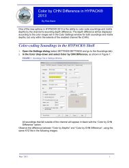
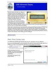
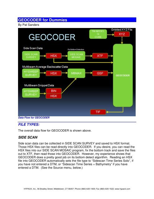
Data Flow <strong>for</strong> GEOCODER<br />
FILE TYPES:<br />
The overall data flow <strong>for</strong> GEOCODER is shown above.<br />
SIDE SCAN<br />
Side scan data can be collected in SIDE SCAN SURVEY and saved to HSX <strong>for</strong>mat.<br />
Those HSX files can be read directly into GEOCODER. If you desire, you can read the<br />
HSX files into our SIDE SCAN MOSAIC program, fix the bottom track and save the files<br />
out to XTF, then read those into GEOCODER. However, my experience shows that<br />
GEOCODER does a pretty good job on its bottom detect algorithm. Reading an HSX<br />
file into GEOCODER automatically sets the file type to “Sidescan Time Series Solo”, if<br />
you have not entered a DTM, or “Sidescan Time Series + Bathymetry” if you have<br />
entered a DTM. (See the Source menu, below.)<br />
HYPACK, Inc., 56 Bradley Street, Middletown, CT 06457; Phone (860)-635-1500; Fax (860)-635-1522; www.hypack.com
MULTIBEAM AVERAGE BACKSCATTER<br />
Average backscatter data can be stored<br />
in the HSX files by the HYSWEEP®<br />
SURVEY program. Those files must be<br />
read into MBMAX and then saved out to<br />
GSF <strong>for</strong>mat (new in the output options) in<br />
order to be read into GEOCODER. The<br />
Source menu should be set to “Beam<br />
Average” be<strong>for</strong>e loading the GSF files.<br />
MULTIBEAM SNIPPETS<br />
The HYSWEEP® SURVEY program stores the snippet data in a Binary file. You<br />
should load the HSX files into MBMAX and then export a GSF file. MBMAX will<br />
automatically read the BIN file and insert the appropriate records in each GSF file. Set<br />
the ‘Source’ to Beam Time Series be<strong>for</strong>e loading your GSF files.<br />
DTMs:<br />
My experience shows that the DTM should be<br />
loaded be<strong>for</strong>e the side scan or backscatter data.<br />
Use the ‘Read XYZ Grid’ function in the DTM menu.<br />
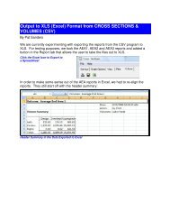
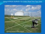
Setting Calibration Parameters:<br />
Be<strong>for</strong>e reading your data files into GEOCODER,<br />
select Edit > Calibration Parameters. Don’t worry<br />
about the offset section, as we take care of all of<br />
this internally. The most important part is the<br />
XTF/SDF Side Scan Options.<br />
• Show if the sensor is located on the main<br />
vessel or the towfish. Check either Ship<br />
Navigation or Sensor Navigation.<br />
• Smooth the point-to-point navigation. We<br />
recommend that you use the Spline Decimation<br />
with a setting of 300.<br />
Models can be improved by applying AVG (Angle Varied<br />
Gain). In order to make use of this function, load an XYZ<br />
data file with fixed spacing between sounding points. To<br />
create these files:<br />
• Save an XYZ file from CUBE<br />
• Save a gridded XYZ file from TIN MODEL, or<br />
• Save values at the<br />
center of each cell<br />
in MAPPER.<br />
HYPACK, Inc., 56 Bradley Street, Middletown, CT 06457; Phone (860)-635-1500; Fax (860)-635-1522; www.hypack.com
• The altitude of the towfish above the bottom can be computed from the Ship<br />
Altitude, Sensor Altitude or Bottom Detection. We have been using the Bottom<br />
Detection <strong>for</strong> most of our testing.<br />
• The orientation of the scan can be either Ship Heading (multibeam systems),<br />
Sensor Heading (towfish with heading indicator) or Course Made Good (towfish –<br />
computed from positions.)<br />
• Channels 0,1 are typically the High Frequency data and Channels 2,3 are typically<br />
the low frequency data. You have to make a choice when reading the data into<br />
GEOCODER.<br />
For some XTF files, you can tell the program whether to apply the layback contained in<br />
the file. You can also fix the layback at a constant distance behind the vessel. If you<br />
use the latter feature, you also need to compute ‘Apply Layback’. I don’t think we<br />
currently make use of the layback features in our XTF output.<br />
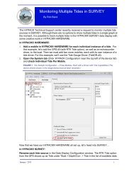
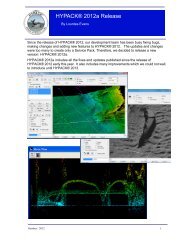
Inserting Files:<br />
1. Select Project > Insert Line.<br />
2. Specify the data type (HSX or GSF or XTF) and<br />
enter one or more files.<br />
GEOCODER will read each file and display the<br />
navigation track and the swath coverage in order to<br />
determine the limits of your mosaic.<br />
To limit the area created by the mosaic, select<br />
Options>Fixed Bounds and specify the X-Y limits (top<br />
left of screen) be<strong>for</strong>e reading in any data files.<br />
GEOCODER does not store any in<strong>for</strong>mation in<br />
memory. It reads through data sequentially and<br />
extracts whatever data it needs.<br />
View Histogram: Be<strong>for</strong>e generating a mosaic, it is<br />
useful to examine the histogram and setting the<br />
bounds. Select View > Historgram and enter the<br />
minimum and maximum dB values to color-code the<br />
mosaic.<br />
Beam Pattern: We do not yet have the capability to<br />
extract the beam pattern. However, we are working<br />
on it and it should be available soon.<br />
Create Mosaic:<br />
Select Mosaic > Assemble. You’ll see the results on<br />
the screen as it runs through each file. GSF files are<br />
processed much faster than HSX or XTF data.<br />
HYPACK, Inc., 56 Bradley St., Middletown CT 06457 USA<br />
Phone (860)-635-1500 Fax (860)-635-1522 Web: www.hypack.com e-mail: sales@hypack.com<br />
3
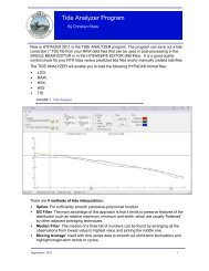
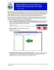
Working on the Mosaic:<br />
Once the mosaic has been assembled, lighten or<br />
darken the area and you can also adjust how the<br />
overlap between adjacent lines is determined. You<br />
can then either adjust the entire line or a section of<br />
the line.<br />
1. Select an individual line you want to work with by<br />
clicking on the navigation track line.<br />
2. Select Mosaic > Remosaic Selected Line.<br />
3. If you want to work with only a portion of the<br />
selected line, enter the ping numbers.<br />
4. To lighten or darken the area, apply a dB offset<br />
5. To adjust how the overlap between adjacent lines<br />
in the selected area is determined. You can<br />
select the appropriate method in the bottom of the<br />
Remosaic dialog box. Among the options:<br />
a. Blend (‘blends the overlap)<br />
b. Fill Gaps (only uses the select line to fill gaps<br />
in the adjacent side scan coverage. Adjacent<br />
lines rule!<br />
c. Forced Overlay (<strong>for</strong>ces the selected file to the<br />
top of the mosaic and it become opaque.<br />
d. Delete (remove the selected file from the<br />
mosaic.<br />
Saving your Mosaic:<br />
Select Mosaic > Save Tiff. <strong>Geocoder</strong> saves your mosaic to a TIF & TFW file pair.<br />
Caveat: During a meeting with Luciano Fonseca, he recommended we remove about<br />
2/3 of the available menu items. Many of them are from research he or his<br />
students were conducting and the results are negligible or can sometimes cause<br />
the program to crash.<br />
HYPACK, Inc., 56 Bradley Street, Middletown, CT 06457; Phone (860)-635-1500; Fax (860)-635-1522; www.hypack.com
ERROR: stackunderflow<br />
OFFENDING COMMAND: begin<br />
STACK: