MOLPRO
MOLPRO
MOLPRO

You also want an ePaper? Increase the reach of your titles
YUMPU automatically turns print PDFs into web optimized ePapers that Google loves.
<strong>MOLPRO</strong><br />
Users Manual<br />
Version 2010.1<br />
H.-J. Werner<br />
Institut für Theoretische Chemie<br />
Universität Stuttgart<br />
Pfaffenwaldring 55<br />
D-70569 Stuttgart<br />
Federal Republic of Germany<br />
P. J. Knowles<br />
School of Chemistry<br />
Cardiff University<br />
Main Building, Park Place, Cardiff CF10 3AT<br />
United Kingdom<br />
SHA1 833379180250ebe11052d872bd9ff53639690c67<br />
(Copyright c○2008 University College Cardiff Consultants Limited)
i<br />
Introduction to <strong>MOLPRO</strong><br />
<strong>MOLPRO</strong> is a complete system of ab initio programs for molecular electronic structure calculations,<br />
designed and maintained by H.-J. Werner and P. J. Knowles, and containing contributions<br />
from a number of other authors. As distinct from other commonly used quantum chemistry<br />
packages, the emphasis is on highly accurate computations, with extensive treatment of the<br />
electron correlation problem through the multiconfiguration-reference CI, coupled cluster and<br />
associated methods. The recently developed explicitly correlated coupled-cluster methods yield<br />
CCSD(T) results with near basis set limit accuracy already with double−ζ or triple−ζ basis<br />
sets, thus reducing the computational effort for calculations of this quality by two orders of<br />
magnitude. Using local electron correlation methods, which significantly reduce the increase<br />
of the computational cost with molecular size, accurate ab initio calculations can be performed<br />
for much larger molecules than with most other programs. These methods have recently been<br />
augmented by explicitly correlated terms, which strongly reduce both the basis set truncation<br />
errors and the errors of the local approximations.<br />
The heart of the program consists of the multiconfiguration SCF, multireference CI, and coupledcluster<br />
routines, and these are accompanied by a full set of supporting features. The package<br />
comprises<br />
• Integral generation for generally contracted symmetry adapted gaussian basis functions<br />
(spd f ghi). There are two programs with identical functionality: the preferred code is<br />
SEWARD (R. Lindh) which is the best on most machines; ARGOS (R. M. Pitzer) is available<br />
as an alternative, and in some cases is optimum for small memory scalar machines.<br />
Also two different gradient integral codes, namely CADPAC (R. Amos) and ALASKA (R.<br />
Lindh) are available. Only the latter allows the use of generally contracted symmetry<br />
adapted gaussian basis functions.<br />
• Effective Core Potentials (contributions from H. Stoll).<br />
• Many one-electron properties.<br />
• Some two-electron properties, e.g. L 2 x, L 2 y, L 2 z , L x L y etc..<br />
• Closed-shell and open-shell (spin restricted and unrestricted) self consistent field.<br />
• Density-functional theory in the Kohn-Sham framework with various gradient corrected<br />
exchange and correlation potentials.<br />
• Multiconfiguration self consistent field. This is the quadratically convergent MCSCF<br />
procedure described in J. Chem. Phys. 82 (1985) 5053. The program can optimize a<br />
weighted energy average of several states, and is capable of treating both completely general<br />
configuration expansions and also long CASSCF expansions as described in Chem.<br />
Phys. Letters 115 (1985) 259.<br />
• Multireference CI. As well as the usual single reference function approaches (MP2, SDCI,<br />
CEPA), this module implements the internally contracted multireference CI method as<br />
described in J. Chem. Phys. 89 (1988) 5803 and Chem. Phys. Lett. 145 (1988) 514. Non<br />
variational variants (e.g. MR-ACPF), as described in Theor. Chim. Acta 78 (1990) 175,<br />
are also available. Electronically excited states can be computed as described in Theor.<br />
Chim. Acta, 84 95 (1992).<br />
• Multireference second-order and third-order perturbation theory (MRPT2, CASPT2, MRPT3)<br />
as described in Mol. Phys. 89, 645 (1996) and J. Chem. Phys. 112, 5546 (2000).
ii<br />
• Møller-Plesset perturbation theory (MPPT), Coupled-Cluster (CCSD), Quadratic configuration<br />
interaction (QCISD), and Brueckner Coupled-Cluster (BCCD) for closed shell<br />
systems, as described in Chem. Phys. Lett. 190 (1992) 1. Perturbative corrections for<br />
triple excitations can also be calculated (Chem. Phys. Letters 227 (1994) 321).<br />
• Open-shell coupled cluster theories as described in J. Chem. Phys. 99 (1993) 5219,<br />
Chem. Phys. Letters 227 (1994) 321.<br />
• An interface to the MRCC program of M. Kallay, allowing coupled-cluster calculations<br />
with arbitrary excitation level.<br />
• Full Configuration Interaction. This is the determinant based benchmarking program described<br />
in Comp. Phys. Commun. 54 (1989) 75.<br />
• Analytical energy gradients for SCF, DFT, state-averaged MCSCF/CASSCF, MRPT2/CASPT2,<br />
MP2 and QCISD(T) methods.<br />
• Analytical non-adiabatic coupling matrix elements for MCSCF.<br />
• Valence-Bond analysis of CASSCF wavefunction, and energy-optimized valence bond<br />
wavefunctions as described in Int. J. Quant. Chem. 65, 439 (1997).<br />
• One-electron transition properties for MCSCF, MRCI, and EOM-CCSD wavefunctions,<br />
CASSCF and MRCI transition properties also between wavefunctions with different orbitals,<br />
as described in Mol. Phys. 105, 1239, (2007).<br />
• Spin-orbit coupling, as described in Mol. Phys., 98, 1823 (2000). More recently, a new<br />
spin-orbit integral program for generally contracted basis sets has been implemented.<br />
• Douglas-Kroll-Hess Hamiltonian up to arbitrary order.<br />
• Density-functional theory symmetry-adapted intermolecular perturbation theory (with density<br />
fitting), DFT-SAPT , as described in J. Chem. Phys. 122, 014103 (2005).<br />
• Some two-electron transition properties for MCSCF wavefunctions (e.g., L 2 x etc.).<br />
• Mulliken population analysis and Natural Population Analysis (NPA)<br />
• Orbital localization.<br />
• Natural bond orbitals (NBOs).<br />
• Distributed Multipole Analysis (A. J. Stone).<br />
• Automatic geometry optimization as described in J. Comp. Chem. 18, (1997), 1473.<br />
Constrained optimization is also possible.<br />
• Automatic calculation of vibrational frequencies, intensities, and thermodynamic properties.<br />
• Reaction path following, as described in Theor. Chem. Acc. 100, (1998), 21.<br />
• Efficient facilities to treat large lattices of point charges for QM/MM calculations, including<br />
lattice gradients.<br />
• Various utilities allowing other more general optimizations, looping and branching (e.g.,<br />
for automatic generation of complete potential energy surfaces), general housekeeping<br />
operations.
iii<br />
• Geometry output in XYZ, MOLDEN and Gaussian formats; molecular orbital and frequency<br />
output in MOLDEN format.<br />
• Integral-direct implementation of all Hartree-Fock, DFT and pair-correlated methods (MP,<br />
CCSD, MRCI etc.), as described in Mol. Phys., 96, (1999), 719. At present, perturbative<br />
triple excitation methods are not implemented.<br />
• Local second-order Møller-Plesset perturbation theory (LMP2) and local coupled cluster<br />
methods, as described in in J. Chem. Phys. 104, 6286 (1996), Chem. Phys. Lett. 290,<br />
143 (1998), J. Chem. Phys. 111, 5691 (1999), J. Chem. Phys. 113, 9443 (2000), J. Chem.<br />
Phys. 113, 9986 (2000), Chem. Phys. Letters 318, 370 (2000), J. Chem. Phys. 114, 661<br />
(2001), Phys. Chem. Chem. Phys. 4, 3941 (2002), J. Chem. Phys. 116, 8772 (2002).<br />
• Local density fitting methods, as described in J. Chem. Phys. 118, 8149 (2003), Phys.<br />
Chem. Chem. Phys. 5, 3349 (2003), Mol. Phys. 102, 2311 (2004).<br />
• Analytical energy gradients for LMP2, DF-LMP2, and LQCISD as described in J. Chem.<br />
Phys. 108, 5185, (1998), Phy. Chem. Chem. Phys. 3, 4853 (2001), J. Chem. Phys. 121,<br />
737 (2004).<br />
• Explicitly correlated MP2-F12 and CCSD(T)-F12 methods, as described in J. Chem.<br />
Phys. 119, 4607 (2003), J. Chem. Phys. 121, 4479 (2004), J. Chem. Phys. 124, 054114<br />
(2006), J. Chem. Phys. 124, 094103 (2006), J. Chem. Phys. 127, 221106 (2007), J.<br />
Chem. Phys. 130, 054104 (2009).<br />
• Explicitly correlated local methods, as described in J. Chem. Phys. 129, 101103 (2009),<br />
J. Chem. Phys. 130, 054106 (2009), J. Chem. Phys. 130, 241101 (2009).<br />
• Parallel execution on distributed memory machines, as described in J. Comp. Chem. 19,<br />
(1998), 1215. At present, SCF, DFT, MRCI, MP2, LMP2, CCSD(T), LCCSD(T) energies<br />
and SCF, DFT gradients are parallelized. Most density fitted codes such as DF-HF, DF-<br />
KS, DF-LMP2, DF-LMP2 gradients, DF-LCCSD(T), DF-MP2-F12, DF-DFT-SAPT, and<br />
GIAO-DF-HF NMR shieldings are also parallelized.<br />
• Automatic embarrassingly parallel computation of numerical gradients and Hessians<br />
(mppx Version).<br />
The program is written mostly in standard Fortran–90. Those parts which are machine dependent<br />
are maintained through the use of a supplied preprocessor, which allows easy interconversion<br />
between versions for different machines. Each release of the program is ported and<br />
tested on a number of systems. A fuller description of the hardware and operating systems of<br />
these machines can be found at http://www.molpro.net/supported. A large library<br />
of commonly used orbital basis sets is available, which can be extended as required. There is a<br />
comprehensive users’ manual, which includes installation instructions. The manual is available<br />
in PDF and also in HTML for mounting on a Worldwide Web server.<br />
More recent methods and enhancements include:<br />
1. Explicitly correlated MP2-F12 (closed-shell) and RMP2-F12 (open-shell) methods with<br />
many many different ansätze, as described in H.-J. Werner, T. B. Adler, and F. R. Manby,<br />
J. Chem. Phys. 126, 164102 (2007) and G. Knizia and H.-J. Werner, J. Chem. Phys. 128,<br />
154103 (2008).<br />
2. Explicitly correlated CCSD(T)-F12 methods as described in T. B. Adler, G. Knizia, and<br />
H.-J. Werner, J. Chem. Phys. 127, 221106 (2007) (closed-shell) and G. Knizia, T. B.<br />
Adler, and H.-J. Werner, J. Chem. Phys. 130, 054104 (2009) (open-shell).
iv<br />
3. Explicitly correlated LMP2-F12 and LCCSD-F12 methods as described in H.-J. Werner,<br />
J. Chem. Phys. 129, 101103 (2009), T. B. Adler, H.-J. Werner, and F. R. Manby, J. Chem.<br />
Phys. 130, 054106 (2009), and T. B. Adler and H.-J. Werner, J. Chem. Phys. 130, 241101<br />
(2009).<br />
4. Natural localized orbitals, NPA and NBO analysis and improved methods for domain<br />
selection in local correlation calculations as described in R. A. Mata and H.-J. Werner,<br />
Mol. Phys. 105, 2753 (2007); see also R. A. Mata and H.-J. Werner, J. Chem. Phys. 125,<br />
184110 (2006).<br />
5. Correlation regions in local correlation calculations as described in R. A. Mata, H.-J.<br />
Werner and M. Schütz, J. Chem. Phys. 128, 144106 (2008).<br />
6. Automated calculation of anharmonic vibrational frequencies and zero-point energies using<br />
VCI methods as described in T. Hrenar, H.-J. Werner, and G. Rauhut, J. Chem. Phys.<br />
126, 134108 (2007) and references therein.<br />
7. Dynamical state weighting as described in M. P. Deskevich and D. J. Nesbitt, and H.-J.<br />
Werner, J. Chem. Phys. 120, 7281 (2004).<br />
8. Coupling of DFT and coupled cluster methods as described in E. Goll, T. Leininger, F. R.<br />
Manby, A. Mitrushchenkov, H.-J. Werner, and H. Stoll, Phys. Chem. Chem. Phys. 10,<br />
3353 (2008) and references therein.<br />
9. NMR chemical shifts using London atomic orbitals for density-fitted Hartree-Fock, as<br />
described in S. Loibl, F.R. Manby, M. Schütz, Mol. Phys. 108, 1362 (2010).<br />
10. Local response methods (LCC2) for computing excitation energies and transition properties<br />
in large molecule as described in D. Kats, T. Korona, M. Schütz, J. Chem. Phys. 125,<br />
104106 (2006), D. Kats, T. Korona, M. Schütz, J. Chem. Phys. 127, 064107 (2007), and<br />
D. Kats, M. Schütz, J. Chem. Phys. 131, 124117 (2009).<br />
11. Automatic basis set extrapolation.<br />
12. Enhanced connections to other programs, including graphical display of output and 3-<br />
dimensional structures.<br />
13. Support for Mac OS X<br />
Future enhancements presently under development include<br />
• Explicitly correlated local coupled cluster methods (closed and open-shell)<br />
• Explicitly correlated CASPT2-F12 and MRCI-F12 methods.<br />
• Analytical energy gradients for CCSD(T) and CCSD(T)-F12.<br />
• Analytic second derivatives for DFT.<br />
• New, more efficient MRCI methods for larger molecules.<br />
• NMR chemical shifts using London atomic orbitals for local MP2.<br />
These features will be included in the base version at later stages. The above list is for information<br />
only, and no representation is made that any of the above will be available within any<br />
particular time.
v<br />
<strong>MOLPRO</strong> on the WWW<br />
The latest information on <strong>MOLPRO</strong>, including program updates, can be found on the worldwide<br />
web at location http://www.molpro.net/.<br />
References<br />
All publications resulting from use of this program must acknowledge the following.<br />
<strong>MOLPRO</strong>, version 2010.1, a package of ab initio programs, H.-J. Werner, P. J. Knowles, G. Knizia,<br />
F. R. Manby, M. Schütz, P. Celani, T. Korona, R. Lindh, A. Mitrushenkov, G. Rauhut, K. R.<br />
Shamasundar, T. B. Adler, R. D. Amos, A. Bernhardsson, A. Berning, D. L. Cooper, M. J. O.<br />
Deegan, A. J. Dobbyn, F. Eckert, E. Goll, C. Hampel, A. Hesselmann, G. Hetzer, T. Hrenar,<br />
G. Jansen, C. Köppl, Y. Liu, A. W. Lloyd, R. A. Mata, A. J. May, S. J. McNicholas,<br />
W. Meyer, M. E. Mura, A. Nicklass, D. P. O’Neill, P. Palmieri, K. Pflüger, R. Pitzer, M. Reiher,<br />
T. Shiozaki, H. Stoll, A. J. Stone, R. Tarroni, T. Thorsteinsson, M. Wang, and A. Wolf, , see<br />
http://www.molpro.net.<br />
Some journals insist on a shorter list of authors; in such a case, the following should be used<br />
instead.<br />
<strong>MOLPRO</strong>, version 2010.1, a package of ab initio programs, H.-J. Werner, P. J. Knowles, G.<br />
Knizia, F. R. Manby, M. Schütz, and others , see http://www.molpro.net.<br />
Depending on which programs are used, the following references should be cited.<br />
Integral evaluation (SEWARD)<br />
R. Lindh, U. Ryu, and B. Liu, J. Chem. Phys. 95, 5889 (1991).<br />
Integral-direct Implementation<br />
M. Schütz, R. Lindh, and H.-J. Werner, Mol. Phys. 96, 719 (1999).<br />
MCSCF/CASSCF:<br />
H.-J. Werner and P. J. Knowles, J. Chem. Phys. 82, 5053 (1985);<br />
P. J. Knowles and H.-J. Werner, Chem. Phys. Lett. 115, 259 (1985).<br />
See also:<br />
H.-J. Werner and W. Meyer, J. Chem. Phys. 73, 2342 (1980);<br />
H.-J. Werner and W. Meyer, J. Chem. Phys. 74, 5794 (1981);<br />
H.-J. Werner, Adv. Chem. Phys. LXIX, 1 (1987).<br />
Internally contracted MRCI:<br />
H.-J. Werner and P.J. Knowles, J. Chem. Phys. 89, 5803 (1988);<br />
P.J. Knowles and H.-J. Werner, Chem. Phys. Lett. 145, 514 (1988).<br />
See also:<br />
H.-J. Werner and E.A. Reinsch, J. Chem. Phys. 76, 3144 (1982);<br />
H.-J. Werner, Adv. Chem. Phys. LXIX, 1 (1987).<br />
Excited states with internally contracted MRCI:<br />
P. J. Knowles and H.-J. Werner, Theor. Chim. Acta 84, 95 (1992).<br />
Internally contracted MR-ACPF, QDVPT, etc:<br />
H.-J. Werner and P. J. Knowles, Theor. Chim Acta 78, 175 (1990).
vi<br />
The original reference to uncontracted MR-ACPF, QDVPT, MR-AQCC are:<br />
R. J. Gdanitz and R. Ahlrichs, Chem. Phys. Lett. 143, 413 (1988);<br />
R. J. Cave and E. R. Davidson, J. Chem. Phys. 89, 6798 (1988);<br />
P. G. Szalay and R. J. Bartlett, Chem. Phys. Lett. 214, 481 (1993).<br />
Multireference perturbation theory (CASPT2/CASPT3):<br />
H.-J. Werner, Mol. Phys. 89, 645 (1996);<br />
P. Celani and H.-J. Werner, J. Chem. Phys. 112, 5546 (2000).<br />
Coupling of multi-reference configuration interaction and multi-reference perturbation<br />
theory, P. Celani, H. Stoll, H.-J. Werner and P. J. Knowles, Mol. Phys. 102, 2369 (2004).<br />
Analytical energy gradients and geometry optimization<br />
Gradient integral evaluation (ALASKA): R. Lindh, Theor. Chim. Acta 85, 423 (1993);<br />
MCSCF gradients: T. Busch, A. Degli Esposti, and H.-J. Werner, J. Chem. Phys. 94, 6708<br />
(1991);<br />
MP2 and LMP2 gradients: A. El Azhary, G. Rauhut, P. Pulay, and H.-J. Werner, J. Chem. Phys.<br />
108, 5185 (1998);<br />
DF-LMP2 gradients: M. Schütz, H.-J. Werner, R. Lindh and F. R. Manby, J. Chem. Phys. 121,<br />
737 (2004).<br />
QCISD and LQCISD gradients: G. Rauhut and H.-J. Werner, Phys. Chem. Chem. Phys. 3,<br />
4853 (2001);<br />
CASPT2 gradients: P. Celani and H.-J. Werner, J. Chem. Phys. 119, 5044 (2003).<br />
Geometry optimization: F. Eckert, P. Pulay and H.-J. Werner, J. Comp. Chemistry 18, 1473<br />
(1997);<br />
Reaction path following: F. Eckert and H.-J. Werner, Theor. Chem. Acc. 100, 21, 1998.<br />
Harmonic frequencies<br />
G. Rauhut, A. El Azhary, F. Eckert, U. Schumann, and H.-J. Werner, Spectrochimica Acta 55,<br />
651 (1999).<br />
T. Hrenar, G. Rauhut, H.-J. Werner, J. Phys. Chem. A 110, 2060 (2006).<br />
Anharmonic frequencies (SURF, VSCF, VCI):<br />
G. Rauhut, J. Chem. Phys. 121, 9313 (2004);<br />
T. Hrenar, H.-J. Werner, G. Rauhut, J. Chem. Phys. 126, 134108 (2007);<br />
G. Rauhut, T. Hrenar, Chem. Phys. 346, 160 (2008);<br />
M. Neff, G. Rauhut, J. Chem. Phys. 131, 124129 (2009).<br />
Møller-Plesset Perturbation theory (MP2, MP3, MP4):<br />
Closed-shell Møller-Plesset Perturbation theory up to fourth order [MP4(SDTQ)] is part of the<br />
coupled cluster code, see CCSD.<br />
Open-shell Møller-Plesset Perturbation theory (RMP2):<br />
R. D. Amos, J. S. Andrews, N. C. Handy, and P. J. Knowles, Chem. Phys. Lett. 185, 256 (1991).<br />
Coupled-Cluster treatments (QCI, CCSD, BCCD):<br />
C. Hampel, K. Peterson, and H.-J. Werner, Chem. Phys. Lett. 190, 1 (1992) and references<br />
therein. The program to compute the perturbative triples corrections has been developed by<br />
M. J. O. Deegan and P. J. Knowles, Chem. Phys. Lett. 227, 321 (1994).<br />
Equation-of-Motion Coupled Cluster Singles and Doubles (EOM-CCSD):<br />
T. Korona and H.-J. Werner, J. Chem. Phys. 118, 3006 (2003).<br />
Open-shell coupled-cluster (RCCSD, UCCSD):<br />
P. J. Knowles, C. Hampel and H.-J. Werner, J. Chem. Phys. 99, 5219 (1993); Erratum: J. Chem.<br />
Phys. 112, 3106 (2000).
vii<br />
Local MP2 (LMP2):<br />
G. Hetzer, P. Pulay, and H.-J. Werner, Chem. Phys. Lett. 290, 143 (1998)<br />
M. Schütz, G. Hetzer, and H.-J. Werner, J. Chem. Phys. 111, 5691 (1999)<br />
G. Hetzer, M. Schütz, H. Stoll, and H.-J. Werner, J. Chem. Phys. 113, 9443 (2000)<br />
See also references on energy gradients and density fitting.<br />
Local Coupled Cluster methods (LCCSD, LQCISD, LMP4):<br />
C. Hampel and H.-J. Werner, J. Chem. Phys. 104 6286 (1996)<br />
M. Schütz and H.-J. Werner, J. Chem. Phys. 114, 661 (2001)<br />
M. Schütz, Phys. Chem. Chem.Phys. 4, 3941 (2002)<br />
See also references on energy gradients and density fitting.<br />
Local triple excitations:<br />
M. Schütz and H.-J. Werner, Chem. Phys. Lett. 318, 370 (2000);<br />
M. Schütz, J. Chem. Phys. 113, 9986 (2000).<br />
M. Schütz, J. Chem. Phys. 116, 8772 (2002).<br />
Density fitting methods:<br />
DFT, Poisson fitting:<br />
DF-MP2, DF-LMP2:<br />
DF-LCCSD:<br />
DF-HF:<br />
DF-LMP2 gradients:<br />
DF-LCCSD(T):<br />
F. R. Manby, P. J. Knowles, and A. W. Lloyd,<br />
J. Chem. Phys. 115, 9144 (2001).<br />
H.-J. Werner, F. R. Manby, and P. J. Knowles,<br />
J. Chem. Phys. 118, 8149 (2003).<br />
M. Schütz and F. R. Manby,<br />
Phys. Chem. Chem. Phys. 5, 3349 (2003)<br />
R. Polly, H.-J. Werner, F. R. Manby, and Peter J. Knowles,<br />
Mol. Phys. 102, 2311 (2004).<br />
M. Schütz, H.-J. Werner, R. Lindh and F. R. Manby,<br />
J. Chem. Phys. 121, 737 (2004).<br />
H.-J. Werner and M. Schütz,<br />
in prepation.<br />
Explicitly correlated methods with density fitting:<br />
DF-MP2-R12: F. R. Manby, J. Chem. Phys. 119, 4807 (2003).<br />
DF-MP2-F12/2A: A. J. May and F. R. Manby, J. Chem. Phys. 121, 4479 (2004).<br />
DF-MP2-F12: H.-J. Werner, T. B. Adler, and F. R. Manby, J. Chem. Phys. 126,<br />
164102 (2007).<br />
DF-RMP2-F12: G. Knizia and H.-J. Werner, J. Chem. Phys. 128, 154103 (2008).<br />
DF-LMP2-F12: H.-J. Werner and F. R. Manby, J. Chem. Phys., 124, 054114 (2006);<br />
F. R. Manby H.-J. Werner, T. B. Adler, and A. J. May, J. Chem. Phys.<br />
124, 094103 (2006); H.-J. Werner, T. B. Adler, and F. R. Manby, J.<br />
Chem. Phys. 126, 164102 (2007); T. B. Adler, H.-J. Werner, and F.<br />
R. Manby, J. Chem. Phys. 130, 054106 (2009).<br />
CCSD(T)-F12: T. B. Adler, G. Knizia, and H.-J. Werner, J. Chem. Phys. 127, 221106<br />
(2007).<br />
UCCSD(T)-F12: G. Knizia, T. B. Adler, and H.-J. Werner, J. Chem. Phys. 130, 054104<br />
(2009).
viii<br />
Rangehybrid methods:<br />
T. Leininger, H. Stoll, H.-J. Werner, and A. Savin, Chem. Phys. Lett. 275, 151 (1997).<br />
J.G. Ángyán, I.C. Gerber, A. Savin, and J. Toulouse, Phys. Rev. A 72, 012510 (2005).<br />
E. Goll, H.-J. Werner, and H. Stoll, Phys. Chem. Chem. Phys. 7, 3917 (2005).<br />
Full CI (FCI):<br />
P. J. Knowles and N. C. Handy, Chem. Phys. Letters 111, 315 (1984);<br />
P. J. Knowles and N. C. Handy, Comp. Phys. Commun. 54, 75 (1989).<br />
Distributed Multipole Analysis (DMA):<br />
A. J. Stone, Chem. Phys. Letters 83, 233 (1981).<br />
Valence bond:<br />
D. L. Cooper, T. Thorsteinsson, and J. Gerratt, Int. J. Quant. Chem. 65, 439 (1997);<br />
D. L. Cooper, T. Thorsteinsson, and J. Gerratt, Adv. Quant. Chem. 32, 51-67 (1998).<br />
See also ”An overview of the CASVB approach to modern valence bond calculations”,<br />
T. Thorsteinsson and D. L. Cooper, in Quantum Systems in Chemistry and Physics. Volume 1:<br />
Basic problems and models systems, eds. A. Hernndez-Laguna, J. Maruani, R. McWeeny, and<br />
S. Wilson (Kluwer, Dordrecht, 2000); pp 303-26.<br />
Relativistic corrections using the Douglas-Kroll Hamiltonian:<br />
M. Reiher, A. Wolf, JCP 121, 2037–2047 (2004);<br />
M. Reiher, A. Wolf, JCP 121, 10945–10956 (2004);<br />
A. Wolf, M. Reiher, B. A. Hess, JCP 117, 9215–9226 (2002).<br />
Spin-orbit coupling:<br />
A. Berning, M. Schweizer, H.-J. Werner, P. J. Knowles, and P. Palmieri, Mol. Phys., 98, 1823<br />
(2000).<br />
Diabatization procedures:<br />
H.-J. Werner and W. Meyer, J. Chem. Phys. 74, 5802 (1981);<br />
H.-J. Werner, B. Follmeg, and M. H. Alexander, J. Chem. Phys. 89, 3139 (1988);<br />
D. Simah, B. Hartke, and H.-J. Werner, J. Chem. Phys. 111, 4523 (1999).<br />
DF-DFT-SAPT:<br />
A. Heßelmann, G. Jansen and M. Schütz, J. Chem. Phys. 122, 014103 (2005).<br />
NMR shielding tensors:<br />
S. Loibl, F.R. Manby, M. Schütz, Mol. Phys. 108, 1362 (2010).
CONTENTS<br />
ix<br />
Contents<br />
1 HOW TO READ THIS MANUAL 1<br />
2 RUNNING <strong>MOLPRO</strong> 1<br />
2.1 Options . . . . . . . . . . . . . . . . . . . . . . . . . . . . . . . . . . . . . . 1<br />
2.2 Running <strong>MOLPRO</strong> on parallel computers . . . . . . . . . . . . . . . . . . . . 3<br />
2.2.1 Specifying parallel execution . . . . . . . . . . . . . . . . . . . . . . . 4<br />
3 DEFINITION OF <strong>MOLPRO</strong> INPUT LANGUAGE 7<br />
3.1 Input format . . . . . . . . . . . . . . . . . . . . . . . . . . . . . . . . . . . . 7<br />
3.2 Commands . . . . . . . . . . . . . . . . . . . . . . . . . . . . . . . . . . . . 8<br />
3.3 Directives . . . . . . . . . . . . . . . . . . . . . . . . . . . . . . . . . . . . . 9<br />
3.4 Global directives . . . . . . . . . . . . . . . . . . . . . . . . . . . . . . . . . 9<br />
3.5 Options . . . . . . . . . . . . . . . . . . . . . . . . . . . . . . . . . . . . . . 10<br />
3.6 Data . . . . . . . . . . . . . . . . . . . . . . . . . . . . . . . . . . . . . . . . 10<br />
3.7 Expressions . . . . . . . . . . . . . . . . . . . . . . . . . . . . . . . . . . . . 10<br />
3.8 Intrinsic functions . . . . . . . . . . . . . . . . . . . . . . . . . . . . . . . . . 11<br />
3.9 Variables . . . . . . . . . . . . . . . . . . . . . . . . . . . . . . . . . . . . . 12<br />
3.9.1 Setting variables . . . . . . . . . . . . . . . . . . . . . . . . . . . . . 12<br />
3.9.2 String variables . . . . . . . . . . . . . . . . . . . . . . . . . . . . . . 12<br />
3.10 Procedures . . . . . . . . . . . . . . . . . . . . . . . . . . . . . . . . . . . . . 13<br />
3.10.1 Procedure definition . . . . . . . . . . . . . . . . . . . . . . . . . . . 13<br />
3.10.2 Procedure calls . . . . . . . . . . . . . . . . . . . . . . . . . . . . . . 13<br />
4 GENERAL PROGRAM STRUCTURE 14<br />
4.1 Input structure . . . . . . . . . . . . . . . . . . . . . . . . . . . . . . . . . . . 14<br />
4.2 Files . . . . . . . . . . . . . . . . . . . . . . . . . . . . . . . . . . . . . . . . 15<br />
4.3 Records . . . . . . . . . . . . . . . . . . . . . . . . . . . . . . . . . . . . . . 15<br />
4.4 Restart . . . . . . . . . . . . . . . . . . . . . . . . . . . . . . . . . . . . . . . 16<br />
4.5 Data set manipulation . . . . . . . . . . . . . . . . . . . . . . . . . . . . . . . 16<br />
4.6 Memory allocation . . . . . . . . . . . . . . . . . . . . . . . . . . . . . . . . 16<br />
4.7 Multiple passes through the input . . . . . . . . . . . . . . . . . . . . . . . . . 16<br />
4.8 Symmetry . . . . . . . . . . . . . . . . . . . . . . . . . . . . . . . . . . . . . 16<br />
4.9 Defining the wavefunction . . . . . . . . . . . . . . . . . . . . . . . . . . . . 18<br />
4.10 Defining orbital subspaces . . . . . . . . . . . . . . . . . . . . . . . . . . . . 19<br />
4.11 Selecting orbitals and density matrices (ORBITAL, DENSITY) . . . . . . . . . 19
CONTENTS<br />
x<br />
4.12 Summary of keywords known to the controlling program . . . . . . . . . . . . 21<br />
4.13 <strong>MOLPRO</strong> help . . . . . . . . . . . . . . . . . . . . . . . . . . . . . . . . . . . 24<br />
5 INTRODUCTORY EXAMPLES 25<br />
5.1 Using the molpro command . . . . . . . . . . . . . . . . . . . . . . . . . . . . 25<br />
5.2 Simple SCF calculations . . . . . . . . . . . . . . . . . . . . . . . . . . . . . 25<br />
5.3 Geometry optimizations . . . . . . . . . . . . . . . . . . . . . . . . . . . . . . 26<br />
5.4 CCSD(T) . . . . . . . . . . . . . . . . . . . . . . . . . . . . . . . . . . . . . 26<br />
5.5 CASSCF and MRCI . . . . . . . . . . . . . . . . . . . . . . . . . . . . . . . 26<br />
5.6 Tables . . . . . . . . . . . . . . . . . . . . . . . . . . . . . . . . . . . . . . . 27<br />
5.7 Procedures . . . . . . . . . . . . . . . . . . . . . . . . . . . . . . . . . . . . . 28<br />
5.8 Do loops . . . . . . . . . . . . . . . . . . . . . . . . . . . . . . . . . . . . . . 28<br />
6 PROGRAM CONTROL 30<br />
6.1 Starting a job (***) . . . . . . . . . . . . . . . . . . . . . . . . . . . . . . . . 30<br />
6.2 Ending a job (---) . . . . . . . . . . . . . . . . . . . . . . . . . . . . . . . . 31<br />
6.3 Restarting a job (RESTART) . . . . . . . . . . . . . . . . . . . . . . . . . . . 31<br />
6.4 Including secondary input files (INCLUDE) . . . . . . . . . . . . . . . . . . . 31<br />
6.5 Allocating dynamic memory (MEMORY) . . . . . . . . . . . . . . . . . . . . . 32<br />
6.6 DO loops (DO/ENDDO) . . . . . . . . . . . . . . . . . . . . . . . . . . . . . . 32<br />
6.6.1 Examples for do loops . . . . . . . . . . . . . . . . . . . . . . . . . . 33<br />
6.7 Branching (IF/ELSEIF/ENDIF) . . . . . . . . . . . . . . . . . . . . . . . . 33<br />
6.7.1 IF statements . . . . . . . . . . . . . . . . . . . . . . . . . . . . . . . 34<br />
6.7.2 GOTO commands . . . . . . . . . . . . . . . . . . . . . . . . . . . . . 34<br />
6.7.3 Labels (LABEL) . . . . . . . . . . . . . . . . . . . . . . . . . . . . . 35<br />
6.8 Procedures (PROC/ENDPROC) . . . . . . . . . . . . . . . . . . . . . . . . . . 35<br />
6.9 Text cards (TEXT) . . . . . . . . . . . . . . . . . . . . . . . . . . . . . . . . . 36<br />
6.10 Checking the program status (STATUS) . . . . . . . . . . . . . . . . . . . . . 37<br />
6.11 Global Thresholds (GTHRESH) . . . . . . . . . . . . . . . . . . . . . . . . . . 37<br />
6.12 Global Print Options (GPRINT/NOGPRINT) . . . . . . . . . . . . . . . . . . 38<br />
6.13 One-electron operators and expectation values (GEXPEC) . . . . . . . . . . . . 39<br />
6.13.1 Example for computing expectation values . . . . . . . . . . . . . . . 40<br />
6.13.2 Example for computing relativistic corrections . . . . . . . . . . . . . 40
CONTENTS<br />
xi<br />
7 FILE HANDLING 43<br />
7.1 FILE . . . . . . . . . . . . . . . . . . . . . . . . . . . . . . . . . . . . . . . 43<br />
7.2 DELETE . . . . . . . . . . . . . . . . . . . . . . . . . . . . . . . . . . . . . . 43<br />
7.3 ERASE . . . . . . . . . . . . . . . . . . . . . . . . . . . . . . . . . . . . . . 43<br />
7.4 DATA . . . . . . . . . . . . . . . . . . . . . . . . . . . . . . . . . . . . . . . 44<br />
7.5 Assigning punch files (PUNCH) . . . . . . . . . . . . . . . . . . . . . . . . . . 44<br />
7.6 <strong>MOLPRO</strong> system parameters (GPARAM) . . . . . . . . . . . . . . . . . . . . 44<br />
8 VARIABLES 45<br />
8.1 Setting variables . . . . . . . . . . . . . . . . . . . . . . . . . . . . . . . . . . 45<br />
8.2 Indexed variables . . . . . . . . . . . . . . . . . . . . . . . . . . . . . . . . . 46<br />
8.3 String variables . . . . . . . . . . . . . . . . . . . . . . . . . . . . . . . . . . 47<br />
8.4 System variables . . . . . . . . . . . . . . . . . . . . . . . . . . . . . . . . . 48<br />
8.5 Macro definitions using string variables . . . . . . . . . . . . . . . . . . . . . 48<br />
8.6 Indexed Variables (Vectors) . . . . . . . . . . . . . . . . . . . . . . . . . . . . 49<br />
8.7 Vector operations . . . . . . . . . . . . . . . . . . . . . . . . . . . . . . . . . 51<br />
8.8 Special variables . . . . . . . . . . . . . . . . . . . . . . . . . . . . . . . . . 51<br />
8.8.1 Variables set by the program . . . . . . . . . . . . . . . . . . . . . . . 51<br />
8.8.2 Variables recognized by the program . . . . . . . . . . . . . . . . . . . 54<br />
8.9 Displaying variables . . . . . . . . . . . . . . . . . . . . . . . . . . . . . . . 57<br />
8.9.1 The SHOW command . . . . . . . . . . . . . . . . . . . . . . . . . . . 57<br />
8.10 Clearing variables . . . . . . . . . . . . . . . . . . . . . . . . . . . . . . . . . 57<br />
8.11 Reading variables from an external file . . . . . . . . . . . . . . . . . . . . . . 58<br />
9 TABLES AND PLOTTING 58<br />
9.1 Tables . . . . . . . . . . . . . . . . . . . . . . . . . . . . . . . . . . . . . . . 58<br />
9.2 Plotting . . . . . . . . . . . . . . . . . . . . . . . . . . . . . . . . . . . . . . 59<br />
9.3 Diatomic potential curve analysis . . . . . . . . . . . . . . . . . . . . . . . . . 61<br />
10 MOLECULAR GEOMETRY 61<br />
10.1 Geometry specifications . . . . . . . . . . . . . . . . . . . . . . . . . . . . . . 61<br />
10.1.1 Z-matrix input . . . . . . . . . . . . . . . . . . . . . . . . . . . . . . 62<br />
10.1.2 XYZ input . . . . . . . . . . . . . . . . . . . . . . . . . . . . . . . . . 63<br />
10.2 Symmetry specification . . . . . . . . . . . . . . . . . . . . . . . . . . . . . . 64<br />
10.3 Writing Gaussian, XMol or MOLDEN input (PUT) . . . . . . . . . . . . . . . 65<br />
10.3.1 Visualization of results using Molden . . . . . . . . . . . . . . . . . . 65
CONTENTS<br />
xii<br />
10.4 Geometry Files . . . . . . . . . . . . . . . . . . . . . . . . . . . . . . . . . . 66<br />
10.5 Lattice of point charges . . . . . . . . . . . . . . . . . . . . . . . . . . . . . . 66<br />
10.6 Redefining and printing atomic masses . . . . . . . . . . . . . . . . . . . . . . 67<br />
10.7 Dummy centres . . . . . . . . . . . . . . . . . . . . . . . . . . . . . . . . . . 67<br />
10.7.1 Counterpoise calculations . . . . . . . . . . . . . . . . . . . . . . . . 68<br />
10.7.2 Example: interaction energy of OH-Ar . . . . . . . . . . . . . . . . . 69<br />
11 BASIS INPUT 69<br />
11.1 Overview: sets and the basis library . . . . . . . . . . . . . . . . . . . . . . . 69<br />
11.2 Cartesian and spherical harmonic basis functions . . . . . . . . . . . . . . . . 70<br />
11.3 The basis set library . . . . . . . . . . . . . . . . . . . . . . . . . . . . . . . . 70<br />
11.4 Default basis sets . . . . . . . . . . . . . . . . . . . . . . . . . . . . . . . . . 71<br />
11.5 Default basis sets for individual atoms . . . . . . . . . . . . . . . . . . . . . . 73<br />
11.6 Basis blocks . . . . . . . . . . . . . . . . . . . . . . . . . . . . . . . . . . . . 73<br />
11.7 Auxiliary basis sets for density fitting or resolution of the identity . . . . . . . 74<br />
11.8 Primitive set definition . . . . . . . . . . . . . . . . . . . . . . . . . . . . . . 74<br />
11.9 Contracted set definitions . . . . . . . . . . . . . . . . . . . . . . . . . . . . . 77<br />
11.10Examples . . . . . . . . . . . . . . . . . . . . . . . . . . . . . . . . . . . . . 77<br />
12 EFFECTIVE CORE POTENTIALS 79<br />
12.1 Input from ECP library . . . . . . . . . . . . . . . . . . . . . . . . . . . . . . 79<br />
12.2 Explicit input for ECPs . . . . . . . . . . . . . . . . . . . . . . . . . . . . . . 79<br />
12.3 Example for explicit ECP input . . . . . . . . . . . . . . . . . . . . . . . . . . 81<br />
12.4 Example for ECP input from library . . . . . . . . . . . . . . . . . . . . . . . 82<br />
13 CORE POLARIZATION POTENTIALS 82<br />
13.1 Input options . . . . . . . . . . . . . . . . . . . . . . . . . . . . . . . . . . . 82<br />
13.2 Example for ECP/CPP . . . . . . . . . . . . . . . . . . . . . . . . . . . . . . 83<br />
14 INTEGRATION 83<br />
14.1 Sorted integrals . . . . . . . . . . . . . . . . . . . . . . . . . . . . . . . . . . 84<br />
14.2 INTEGRAL-DIRECT CALCULATIONS (GDIRECT) . . . . . . . . . . . . . 85<br />
14.2.1 Example for integral-direct calculations . . . . . . . . . . . . . . . . . 93
CONTENTS<br />
xiii<br />
15 DENSITY FITTING 93<br />
15.1 Options for density fitting . . . . . . . . . . . . . . . . . . . . . . . . . . . . . 94<br />
15.1.1 Options to select the fitting basis sets . . . . . . . . . . . . . . . . . . 94<br />
15.1.2 Screening thresholds . . . . . . . . . . . . . . . . . . . . . . . . . . . 95<br />
15.1.3 Parameters to enable local fitting . . . . . . . . . . . . . . . . . . . . . 95<br />
15.1.4 Parameters for fitting domains . . . . . . . . . . . . . . . . . . . . . . 96<br />
15.1.5 Miscellaneous control options . . . . . . . . . . . . . . . . . . . . . . 97<br />
16 THE SCF PROGRAM 98<br />
16.1 Options . . . . . . . . . . . . . . . . . . . . . . . . . . . . . . . . . . . . . . 98<br />
16.1.1 Options to control HF convergence . . . . . . . . . . . . . . . . . . . 98<br />
16.1.2 Options for the diagonalization method . . . . . . . . . . . . . . . . . 99<br />
16.1.3 Options for convergence acceleration methods (DIIS) . . . . . . . . . . 99<br />
16.1.4 Options for integral direct calculations . . . . . . . . . . . . . . . . . . 100<br />
16.1.5 Special options for UHF calculations . . . . . . . . . . . . . . . . . . 100<br />
16.1.6 Options for local density-fitting calculations . . . . . . . . . . . . . . . 100<br />
16.1.7 Options for polarizabilities . . . . . . . . . . . . . . . . . . . . . . . . 100<br />
16.1.8 Printing options . . . . . . . . . . . . . . . . . . . . . . . . . . . . . . 101<br />
16.2 Defining the wavefunction . . . . . . . . . . . . . . . . . . . . . . . . . . . . 101<br />
16.2.1 Defining the number of occupied orbitals in each symmetry . . . . . . 101<br />
16.2.2 Specifying closed-shell orbitals . . . . . . . . . . . . . . . . . . . . . 101<br />
16.2.3 Specifying open-shell orbitals . . . . . . . . . . . . . . . . . . . . . . 101<br />
16.3 Saving the final orbitals . . . . . . . . . . . . . . . . . . . . . . . . . . . . . . 102<br />
16.4 Starting orbitals . . . . . . . . . . . . . . . . . . . . . . . . . . . . . . . . . . 102<br />
16.4.1 Initial orbital guess . . . . . . . . . . . . . . . . . . . . . . . . . . . . 102<br />
16.4.2 Starting with previous orbitals . . . . . . . . . . . . . . . . . . . . . . 103<br />
16.4.3 Starting with a previous density matrix . . . . . . . . . . . . . . . . . 104<br />
16.5 Rotating pairs of orbitals . . . . . . . . . . . . . . . . . . . . . . . . . . . . . 104<br />
16.6 Using additional point-group symmetry . . . . . . . . . . . . . . . . . . . . . 105<br />
16.7 Expectation values . . . . . . . . . . . . . . . . . . . . . . . . . . . . . . . . 105<br />
16.8 Polarizabilities . . . . . . . . . . . . . . . . . . . . . . . . . . . . . . . . . . 105<br />
16.9 Miscellaneous directives . . . . . . . . . . . . . . . . . . . . . . . . . . . . . 105<br />
16.9.1 Level shifts . . . . . . . . . . . . . . . . . . . . . . . . . . . . . . . . 106<br />
16.9.2 Maximum number of iterations . . . . . . . . . . . . . . . . . . . . . 106<br />
16.9.3 Convergence threshold . . . . . . . . . . . . . . . . . . . . . . . . . . 106
CONTENTS<br />
xiv<br />
16.9.4 Sanity check on the energy . . . . . . . . . . . . . . . . . . . . . . . . 106<br />
16.9.5 Print options . . . . . . . . . . . . . . . . . . . . . . . . . . . . . . . 106<br />
16.9.6 Interpolation . . . . . . . . . . . . . . . . . . . . . . . . . . . . . . . 106<br />
16.9.7 Reorthonormalization of the orbitals . . . . . . . . . . . . . . . . . . . 107<br />
16.9.8 Direct SCF . . . . . . . . . . . . . . . . . . . . . . . . . . . . . . . . 107<br />
17 THE DENSITY FUNCTIONAL PROGRAM 108<br />
17.1 Options . . . . . . . . . . . . . . . . . . . . . . . . . . . . . . . . . . . . . . 108<br />
17.2 Directives . . . . . . . . . . . . . . . . . . . . . . . . . . . . . . . . . . . . . 109<br />
17.2.1 Density source (DENSITY, ODENSITY) . . . . . . . . . . . . . . . . 109<br />
17.2.2 Thresholds (DFTTHRESH) . . . . . . . . . . . . . . . . . . . . . . . . 109<br />
17.2.3 Exact exchange computation (EXCHANGE) . . . . . . . . . . . . . . . 109<br />
17.2.4 Rangehybrid methods (RANGEHYBRID) . . . . . . . . . . . . . . . . 110<br />
17.2.5 Exchange-correlation potential (POTENTIAL) . . . . . . . . . . . . . 110<br />
17.2.6 Grid blocking factor (DFTBLOCK) . . . . . . . . . . . . . . . . . . . . 110<br />
17.2.7 Dump integrand values(DFTDUMP) . . . . . . . . . . . . . . . . . . . 110<br />
17.3 Numerical integration grid control (GRID) . . . . . . . . . . . . . . . . . . . . 110<br />
17.3.1 Target quadrature accuracy (GRIDTHRESH) . . . . . . . . . . . . . . . 111<br />
17.3.2 Radial integration grid (RADIAL) . . . . . . . . . . . . . . . . . . . . 111<br />
17.3.3 Angular integration grid (ANGULAR) . . . . . . . . . . . . . . . . . . 112<br />
17.3.4 Atom partitioning of integration grid (VORONOI) . . . . . . . . . . . . 113<br />
17.3.5 Grid caching (GRIDSAVE, NOGRIDSAVE) . . . . . . . . . . . . . . 113<br />
17.3.6 Grid symmetry (GRIDSYM,NOGRIDSYM) . . . . . . . . . . . . . . . 113<br />
17.3.7 Grid printing (GRIDPRINT) . . . . . . . . . . . . . . . . . . . . . . . 113<br />
17.4 Density Functionals . . . . . . . . . . . . . . . . . . . . . . . . . . . . . . . . 114<br />
17.4.1 Alias density functionals . . . . . . . . . . . . . . . . . . . . . . . . . 120<br />
17.4.2 Implementing new functionals . . . . . . . . . . . . . . . . . . . . . . 121<br />
17.4.3 Implementing new hybrid-functionals . . . . . . . . . . . . . . . . . . 122<br />
17.5 Empirical damped dispersion correction . . . . . . . . . . . . . . . . . . . . . 122<br />
17.6 Examples . . . . . . . . . . . . . . . . . . . . . . . . . . . . . . . . . . . . . 123<br />
18 ORBITAL LOCALIZATION 124<br />
18.1 Defining the input orbitals (ORBITAL) . . . . . . . . . . . . . . . . . . . . . . 124<br />
18.2 Saving the localized orbitals (SAVE) . . . . . . . . . . . . . . . . . . . . . . . 124<br />
18.3 Choosing the localization method (METHOD) . . . . . . . . . . . . . . . . . . 125<br />
18.4 Delocalization of orbitals (DELOCAL) . . . . . . . . . . . . . . . . . . . . . . 125
CONTENTS<br />
xv<br />
18.5 Localizing AOs(LOCAO) . . . . . . . . . . . . . . . . . . . . . . . . . . . . . 125<br />
18.6 Selecting the orbital space . . . . . . . . . . . . . . . . . . . . . . . . . . . . 125<br />
18.6.1 Defining the occupied space (OCC) . . . . . . . . . . . . . . . . . . . 125<br />
18.6.2 Defining the core orbitals (CORE) . . . . . . . . . . . . . . . . . . . . 125<br />
18.6.3 Defining groups of orbitals (GROUP, OFFDIAG) . . . . . . . . . . . . 125<br />
18.6.4 Localization between groups (OFFDIAG) . . . . . . . . . . . . . . . . 126<br />
18.7 Ordering of localized orbitals . . . . . . . . . . . . . . . . . . . . . . . . . . . 126<br />
18.7.1 No reordering (NOORDER) . . . . . . . . . . . . . . . . . . . . . . . . 126<br />
18.7.2 Ordering using domains (SORT) . . . . . . . . . . . . . . . . . . . . . 126<br />
18.7.3 Defining reference orbitals (REFORB) . . . . . . . . . . . . . . . . . . 127<br />
18.7.4 Selecting the fock matrix (FOCK) . . . . . . . . . . . . . . . . . . . . 127<br />
18.7.5 Selecting a density matrix (DENSITY) . . . . . . . . . . . . . . . . . 127<br />
18.8 Localization thresholds (THRESH) . . . . . . . . . . . . . . . . . . . . . . . . 127<br />
18.9 Options for PM localization (PIPEK) . . . . . . . . . . . . . . . . . . . . . . 128<br />
18.10Printing options (PRINT) . . . . . . . . . . . . . . . . . . . . . . . . . . . . . 128<br />
19 THE MCSCF PROGRAM MULTI 129<br />
19.1 Structure of the input . . . . . . . . . . . . . . . . . . . . . . . . . . . . . . . 129<br />
19.2 Defining the orbital subspaces . . . . . . . . . . . . . . . . . . . . . . . . . . 130<br />
19.2.1 Occupied orbitals . . . . . . . . . . . . . . . . . . . . . . . . . . . . . 130<br />
19.2.2 Frozen-core orbitals . . . . . . . . . . . . . . . . . . . . . . . . . . . 130<br />
19.2.3 Closed-shell orbitals . . . . . . . . . . . . . . . . . . . . . . . . . . . 131<br />
19.2.4 Freezing orbitals . . . . . . . . . . . . . . . . . . . . . . . . . . . . . 131<br />
19.3 Defining the optimized states . . . . . . . . . . . . . . . . . . . . . . . . . . . 131<br />
19.3.1 Defining the state symmetry . . . . . . . . . . . . . . . . . . . . . . . 131<br />
19.3.2 Defining the number of states in the present symmetry . . . . . . . . . 132<br />
19.3.3 Specifying weights in state-averaged calculations . . . . . . . . . . . . 132<br />
19.3.4 Dynamical weighting . . . . . . . . . . . . . . . . . . . . . . . . . . . 132<br />
19.4 Defining the configuration space . . . . . . . . . . . . . . . . . . . . . . . . . 132<br />
19.4.1 Occupation restrictions . . . . . . . . . . . . . . . . . . . . . . . . . . 132<br />
19.4.2 Selecting configurations . . . . . . . . . . . . . . . . . . . . . . . . . 133<br />
19.4.3 Specifying orbital configurations . . . . . . . . . . . . . . . . . . . . . 133<br />
19.4.4 Selecting the primary configuration set . . . . . . . . . . . . . . . . . 134<br />
19.4.5 Projection to specific Λ states in linear molecules . . . . . . . . . . . . 134<br />
19.5 Restoring and saving the orbitals and CI vectors . . . . . . . . . . . . . . . . . 134
CONTENTS<br />
xvi<br />
19.5.1 Defining the starting guess . . . . . . . . . . . . . . . . . . . . . . . . 135<br />
19.5.2 Rotating pairs of initial orbitals . . . . . . . . . . . . . . . . . . . . . 135<br />
19.5.3 Saving the final orbitals . . . . . . . . . . . . . . . . . . . . . . . . . 135<br />
19.5.4 Saving the CI vectors and information for a gradient calculation . . . . 136<br />
19.5.5 Natural orbitals . . . . . . . . . . . . . . . . . . . . . . . . . . . . . . 136<br />
19.5.6 Pseudo-canonical orbitals . . . . . . . . . . . . . . . . . . . . . . . . 137<br />
19.5.7 Localized orbitals . . . . . . . . . . . . . . . . . . . . . . . . . . . . . 137<br />
19.5.8 Diabatic orbitals . . . . . . . . . . . . . . . . . . . . . . . . . . . . . 137<br />
19.6 Selecting the optimization methods . . . . . . . . . . . . . . . . . . . . . . . . 139<br />
19.6.1 Selecting the CI method . . . . . . . . . . . . . . . . . . . . . . . . . 139<br />
19.6.2 Selecting the orbital optimization method . . . . . . . . . . . . . . . . 140<br />
19.6.3 Disabling the optimization . . . . . . . . . . . . . . . . . . . . . . . . 140<br />
19.6.4 Disabling the extra symmetry mechanism . . . . . . . . . . . . . . . . 140<br />
19.7 Calculating expectation values . . . . . . . . . . . . . . . . . . . . . . . . . . 141<br />
19.7.1 Matrix elements over one-electron operators . . . . . . . . . . . . . . . 141<br />
19.7.2 Matrix elements over two-electron operators . . . . . . . . . . . . . . 141<br />
19.7.3 Saving the density matrix . . . . . . . . . . . . . . . . . . . . . . . . . 141<br />
19.8 Miscellaneous options . . . . . . . . . . . . . . . . . . . . . . . . . . . . . . 141<br />
19.8.1 Print options . . . . . . . . . . . . . . . . . . . . . . . . . . . . . . . 142<br />
19.8.2 Convergence thresholds . . . . . . . . . . . . . . . . . . . . . . . . . 142<br />
19.8.3 Maximum number of iterations . . . . . . . . . . . . . . . . . . . . . 143<br />
19.8.4 Test options . . . . . . . . . . . . . . . . . . . . . . . . . . . . . . . . 143<br />
19.8.5 Special optimization parameters . . . . . . . . . . . . . . . . . . . . . 143<br />
19.8.6 Saving wavefunction information for CASVB . . . . . . . . . . . . . . 144<br />
19.8.7 Saving transformed integrals . . . . . . . . . . . . . . . . . . . . . . . 144<br />
19.9 Coupled-perturbed MCSCF . . . . . . . . . . . . . . . . . . . . . . . . . . . . 144<br />
19.9.1 Gradients for SA-MCSCF . . . . . . . . . . . . . . . . . . . . . . . . 145<br />
19.9.2 Difference gradients for SA-MCSCF . . . . . . . . . . . . . . . . . . 145<br />
19.9.3 Non-adiabatic coupling matrix elements for SA-MCSCF . . . . . . . . 145<br />
19.9.4 MCSCF hessians . . . . . . . . . . . . . . . . . . . . . . . . . . . . . 146<br />
19.10Optimizing valence bond wavefunctions . . . . . . . . . . . . . . . . . . . . . 146<br />
19.11Hints and strategies . . . . . . . . . . . . . . . . . . . . . . . . . . . . . . . . 146<br />
19.12Examples . . . . . . . . . . . . . . . . . . . . . . . . . . . . . . . . . . . . . 147
CONTENTS<br />
xvii<br />
20 THE CI PROGRAM 148<br />
20.1 Introduction . . . . . . . . . . . . . . . . . . . . . . . . . . . . . . . . . . . . 149<br />
20.2 Specifying the wavefunction . . . . . . . . . . . . . . . . . . . . . . . . . . . 149<br />
20.2.1 Occupied orbitals . . . . . . . . . . . . . . . . . . . . . . . . . . . . . 149<br />
20.2.2 Frozen-core orbitals . . . . . . . . . . . . . . . . . . . . . . . . . . . 149<br />
20.2.3 Closed-shell orbitals . . . . . . . . . . . . . . . . . . . . . . . . . . . 149<br />
20.2.4 Defining the orbitals . . . . . . . . . . . . . . . . . . . . . . . . . . . 150<br />
20.2.5 Defining the state symmetry . . . . . . . . . . . . . . . . . . . . . . . 150<br />
20.2.6 Additional reference symmetries . . . . . . . . . . . . . . . . . . . . . 150<br />
20.2.7 Selecting configurations . . . . . . . . . . . . . . . . . . . . . . . . . 151<br />
20.2.8 Occupation restrictions . . . . . . . . . . . . . . . . . . . . . . . . . . 152<br />
20.2.9 Explicitly specifying reference configurations . . . . . . . . . . . . . . 152<br />
20.2.10 Defining state numbers . . . . . . . . . . . . . . . . . . . . . . . . . . 152<br />
20.2.11 Defining reference state numbers . . . . . . . . . . . . . . . . . . . . . 153<br />
20.2.12 Specifying correlation of orbital pairs . . . . . . . . . . . . . . . . . . 153<br />
20.2.13 Restriction of classes of excitations . . . . . . . . . . . . . . . . . . . 154<br />
20.3 Options . . . . . . . . . . . . . . . . . . . . . . . . . . . . . . . . . . . . . . 154<br />
20.3.1 Coupled Electron Pair Approximation . . . . . . . . . . . . . . . . . . 154<br />
20.3.2 Coupled Pair Functional (ACPF, AQCC) . . . . . . . . . . . . . . . . 154<br />
20.3.3 Projected excited state calculations . . . . . . . . . . . . . . . . . . . 155<br />
20.3.4 Transition matrix element options . . . . . . . . . . . . . . . . . . . . 155<br />
20.3.5 Convergence thresholds . . . . . . . . . . . . . . . . . . . . . . . . . 155<br />
20.3.6 Level shifts . . . . . . . . . . . . . . . . . . . . . . . . . . . . . . . . 155<br />
20.3.7 Maximum number of iterations . . . . . . . . . . . . . . . . . . . . . 155<br />
20.3.8 Restricting numbers of expansion vectors . . . . . . . . . . . . . . . . 156<br />
20.3.9 Selecting the primary configuration set . . . . . . . . . . . . . . . . . 156<br />
20.3.10 Canonicalizing external orbitals . . . . . . . . . . . . . . . . . . . . . 156<br />
20.3.11 Saving the wavefunction . . . . . . . . . . . . . . . . . . . . . . . . . 156<br />
20.3.12 Starting wavefunction . . . . . . . . . . . . . . . . . . . . . . . . . . 157<br />
20.3.13 One electron properties . . . . . . . . . . . . . . . . . . . . . . . . . . 157<br />
20.3.14 Transition moment calculations . . . . . . . . . . . . . . . . . . . . . 157<br />
20.3.15 Saving the density matrix . . . . . . . . . . . . . . . . . . . . . . . . . 157<br />
20.3.16 Natural orbitals . . . . . . . . . . . . . . . . . . . . . . . . . . . . . . 157<br />
20.3.17 Miscellaneous options . . . . . . . . . . . . . . . . . . . . . . . . . . 158<br />
20.3.18 Miscellaneous parameters . . . . . . . . . . . . . . . . . . . . . . . . 159
CONTENTS<br />
xviii<br />
20.4 Miscellaneous thresholds . . . . . . . . . . . . . . . . . . . . . . . . . . . . . 159<br />
20.5 Print options . . . . . . . . . . . . . . . . . . . . . . . . . . . . . . . . . . . . 160<br />
20.6 Examples . . . . . . . . . . . . . . . . . . . . . . . . . . . . . . . . . . . . . 162<br />
20.7 Cluster corrections for multi-state MRCI . . . . . . . . . . . . . . . . . . . . . 163<br />
21 MULTIREFERENCE RAYLEIGH SCHRÖDINGER PERTURBATION THEORY165<br />
21.1 Introduction . . . . . . . . . . . . . . . . . . . . . . . . . . . . . . . . . . . . 166<br />
21.2 Excited state calculations . . . . . . . . . . . . . . . . . . . . . . . . . . . . . 167<br />
21.3 Multi-State CASPT2 . . . . . . . . . . . . . . . . . . . . . . . . . . . . . . . 167<br />
21.3.1 Performing SS-SR-CASPT2 calculations . . . . . . . . . . . . . . . . 168<br />
21.3.2 Performing MS-MR-CASPT2 calculations . . . . . . . . . . . . . . . 170<br />
21.4 Modified Fock-operators in the zeroth-order Hamiltonian. . . . . . . . . . . . . 171<br />
21.5 Level shifts . . . . . . . . . . . . . . . . . . . . . . . . . . . . . . . . . . . . 171<br />
21.6 Integral direct calculations . . . . . . . . . . . . . . . . . . . . . . . . . . . . 172<br />
21.7 CASPT2 gradients . . . . . . . . . . . . . . . . . . . . . . . . . . . . . . . . 172<br />
21.8 Coupling MRCI and MRPT2: The CIPT2 method . . . . . . . . . . . . . . . . 175<br />
21.9 Further options for CASPT2 and CASPT3 . . . . . . . . . . . . . . . . . . . . 175<br />
22 NEVPT2 calculations 176<br />
22.1 General considerations . . . . . . . . . . . . . . . . . . . . . . . . . . . . . . 176<br />
22.2 Input description . . . . . . . . . . . . . . . . . . . . . . . . . . . . . . . . . 177<br />
23 MØLLER PLESSET PERTURBATION THEORY 178<br />
23.1 Expectation values for MP2 . . . . . . . . . . . . . . . . . . . . . . . . . . . . 179<br />
23.2 Polarizabilities and second-order properties for MP2 . . . . . . . . . . . . . . 179<br />
23.3 CPHF for gradients, expectation values and polarizabilities . . . . . . . . . . . 179<br />
23.4 Density-fitting MP2 (DF-MP2, RI-MP2) . . . . . . . . . . . . . . . . . . . . . 180<br />
23.5 Spin-component scaled MP2 (SCS-MP2) . . . . . . . . . . . . . . . . . . . . 180<br />
24 THE CLOSED SHELL CCSD PROGRAM 182<br />
24.1 Coupled-cluster, CCSD . . . . . . . . . . . . . . . . . . . . . . . . . . . . . . 182<br />
24.2 Quadratic configuration interaction, QCI . . . . . . . . . . . . . . . . . . . . . 183<br />
24.3 Brueckner coupled-cluster calculations, BCCD . . . . . . . . . . . . . . . . . 183<br />
24.3.1 The BRUECKNER directive . . . . . . . . . . . . . . . . . . . . . . . . 183<br />
24.4 Singles-doubles configuration interaction, CISD . . . . . . . . . . . . . . . . . 184<br />
24.5 The DIIS directive . . . . . . . . . . . . . . . . . . . . . . . . . . . . . . . . 184<br />
24.6 Examples . . . . . . . . . . . . . . . . . . . . . . . . . . . . . . . . . . . . . 184
CONTENTS<br />
xix<br />
24.6.1 Single-reference correlation treatments for H 2 O . . . . . . . . . . . . . 184<br />
24.6.2 Single-reference correlation treatments for N 2 F 2 . . . . . . . . . . . . 185<br />
24.7 Saving the density matrix . . . . . . . . . . . . . . . . . . . . . . . . . . . . . 185<br />
24.8 Natural orbitals . . . . . . . . . . . . . . . . . . . . . . . . . . . . . . . . . . 186<br />
24.9 Dual basis set calculations . . . . . . . . . . . . . . . . . . . . . . . . . . . . 187<br />
25 EXCITED STATES WITH EQUATION-OF-MOTION CCSD (EOM-CCSD) 188<br />
25.1 Options for EOM . . . . . . . . . . . . . . . . . . . . . . . . . . . . . . . . . . 188<br />
25.2 Options for EOMPAR card . . . . . . . . . . . . . . . . . . . . . . . . . . . . . 189<br />
25.3 Options for EOMPRINT card . . . . . . . . . . . . . . . . . . . . . . . . . . . 190<br />
25.4 Examples . . . . . . . . . . . . . . . . . . . . . . . . . . . . . . . . . . . . . 191<br />
25.4.1 PES for lowest excited states for hydrogen fluride . . . . . . . . . . . . 191<br />
25.4.2 EOM-CCSD transition moments for hydrogen fluoride . . . . . . . . . 191<br />
25.4.3 Calculate an EOM-CCSD state most similar to a given CIS state . . . . 192<br />
25.5 Excited states with CIS . . . . . . . . . . . . . . . . . . . . . . . . . . . . . . 193<br />
25.6 First- and second-order properties for CCSD . . . . . . . . . . . . . . . . . . . 193<br />
26 OPEN-SHELL COUPLED CLUSTER THEORIES 195<br />
27 The MRCC program of M. Kallay (MRCC) 196<br />
27.1 Installing MRCC . . . . . . . . . . . . . . . . . . . . . . . . . . . . . . . . . . 196<br />
27.2 Running MRCC . . . . . . . . . . . . . . . . . . . . . . . . . . . . . . . . . . 196<br />
28 SMILES 201<br />
28.1 INTERNAL BASIS SETS . . . . . . . . . . . . . . . . . . . . . . . . . . . . 202<br />
28.2 EXTERNAL BASIS SETS . . . . . . . . . . . . . . . . . . . . . . . . . . . . 202<br />
28.3 Example . . . . . . . . . . . . . . . . . . . . . . . . . . . . . . . . . . . . . . 203<br />
29 LOCAL CORRELATION TREATMENTS 204<br />
29.1 Introduction . . . . . . . . . . . . . . . . . . . . . . . . . . . . . . . . . . . . 204<br />
29.2 Getting started . . . . . . . . . . . . . . . . . . . . . . . . . . . . . . . . . . . 205<br />
29.3 Summary of options . . . . . . . . . . . . . . . . . . . . . . . . . . . . . . . . 206<br />
29.4 Summary of directives . . . . . . . . . . . . . . . . . . . . . . . . . . . . . . 209<br />
29.5 General Options . . . . . . . . . . . . . . . . . . . . . . . . . . . . . . . . . . 209<br />
29.6 Options for selection of domains . . . . . . . . . . . . . . . . . . . . . . . . . 212<br />
29.6.1 Standard domains . . . . . . . . . . . . . . . . . . . . . . . . . . . . . 212<br />
29.6.2 Extended domains . . . . . . . . . . . . . . . . . . . . . . . . . . . . 213
CONTENTS<br />
xx<br />
29.6.3 Manually Defining orbital domains (DOMAIN) . . . . . . . . . . . . . 214<br />
29.7 Options for selection of pair classes . . . . . . . . . . . . . . . . . . . . . . . 214<br />
29.8 Directives . . . . . . . . . . . . . . . . . . . . . . . . . . . . . . . . . . . . . 215<br />
29.8.1 The LOCAL directive . . . . . . . . . . . . . . . . . . . . . . . . . . . 215<br />
29.8.2 The MULTP directive . . . . . . . . . . . . . . . . . . . . . . . . . . . 216<br />
29.8.3 Saving the wavefunction (SAVE) . . . . . . . . . . . . . . . . . . . . . 216<br />
29.8.4 Restarting a calculation (START) . . . . . . . . . . . . . . . . . . . . 216<br />
29.8.5 Correlating subsets of electrons (REGION) . . . . . . . . . . . . . . . 216<br />
29.8.6 Domain Merging (MERGEDOM) . . . . . . . . . . . . . . . . . . . . . 217<br />
29.8.7 Energy partitioning for molecular cluster calculations (ENEPART) . . . 217<br />
29.9 Doing it right . . . . . . . . . . . . . . . . . . . . . . . . . . . . . . . . . . . 218<br />
29.9.1 Basis sets . . . . . . . . . . . . . . . . . . . . . . . . . . . . . . . . . 219<br />
29.9.2 Symmetry and Orientation . . . . . . . . . . . . . . . . . . . . . . . . 219<br />
29.9.3 Localization . . . . . . . . . . . . . . . . . . . . . . . . . . . . . . . . 219<br />
29.9.4 Orbital domains . . . . . . . . . . . . . . . . . . . . . . . . . . . . . . 220<br />
29.9.5 Freezing domains . . . . . . . . . . . . . . . . . . . . . . . . . . . . . 221<br />
29.9.6 Pair Classes . . . . . . . . . . . . . . . . . . . . . . . . . . . . . . . . 221<br />
29.9.7 Gradients and frequency calculations . . . . . . . . . . . . . . . . . . 222<br />
29.9.8 Intermolecular interactions . . . . . . . . . . . . . . . . . . . . . . . . 223<br />
29.10Density-fitted LMP2 (DF-LMP2) and coupled cluster (DF-LCCSD(T0)) . . . 223<br />
30 LOCAL METHODS FOR EXCITED STATES 224<br />
30.1 Local CC2 and ADC(2) . . . . . . . . . . . . . . . . . . . . . . . . . . . . . . 224<br />
30.2 Options for EOM . . . . . . . . . . . . . . . . . . . . . . . . . . . . . . . . . . 225<br />
30.3 Parameters on LAPLACE card . . . . . . . . . . . . . . . . . . . . . . . . . . 226<br />
30.4 Print options . . . . . . . . . . . . . . . . . . . . . . . . . . . . . . . . . . . . 226<br />
30.5 Examples . . . . . . . . . . . . . . . . . . . . . . . . . . . . . . . . . . . . . 227<br />
31 EXPLICITLY CORRELATED METHODS 228<br />
31.1 Reference functions . . . . . . . . . . . . . . . . . . . . . . . . . . . . . . . . 230<br />
31.2 Wave function Ansätze . . . . . . . . . . . . . . . . . . . . . . . . . . . . . . 230<br />
31.2.1 The general ansatz . . . . . . . . . . . . . . . . . . . . . . . . . . . . 230<br />
31.2.2 The diagonal ansatz (D) . . . . . . . . . . . . . . . . . . . . . . . . . 230<br />
31.2.3 The fixed amplitude ansatz (FIX) . . . . . . . . . . . . . . . . . . . . 231<br />
31.3 RI Approximations . . . . . . . . . . . . . . . . . . . . . . . . . . . . . . . . 231<br />
31.4 Basis sets . . . . . . . . . . . . . . . . . . . . . . . . . . . . . . . . . . . . . 231
CONTENTS<br />
xxi<br />
31.5 Symmetry . . . . . . . . . . . . . . . . . . . . . . . . . . . . . . . . . . . . . 233<br />
31.6 Options . . . . . . . . . . . . . . . . . . . . . . . . . . . . . . . . . . . . . . 233<br />
31.7 Choosing the ansatz and the level of approximation . . . . . . . . . . . . . . . 236<br />
31.8 CABS Singles correction . . . . . . . . . . . . . . . . . . . . . . . . . . . . . 238<br />
31.9 Pair specific geminal exponents . . . . . . . . . . . . . . . . . . . . . . . . . . 238<br />
31.10CCSD(T)-F12 . . . . . . . . . . . . . . . . . . . . . . . . . . . . . . . . . . . 240<br />
31.11DF-LMP2-F12 calculations with local approximations . . . . . . . . . . . . . 240<br />
31.12Variables set by the F12 programs . . . . . . . . . . . . . . . . . . . . . . . . 242<br />
32 THE FULL CI PROGRAM 244<br />
32.1 Defining the orbitals . . . . . . . . . . . . . . . . . . . . . . . . . . . . . . . 244<br />
32.2 Occupied orbitals . . . . . . . . . . . . . . . . . . . . . . . . . . . . . . . . . 244<br />
32.3 Frozen-core orbitals . . . . . . . . . . . . . . . . . . . . . . . . . . . . . . . . 244<br />
32.4 Defining the state symmetry . . . . . . . . . . . . . . . . . . . . . . . . . . . 244<br />
32.5 Printing options . . . . . . . . . . . . . . . . . . . . . . . . . . . . . . . . . . 245<br />
32.6 Interface to other programs . . . . . . . . . . . . . . . . . . . . . . . . . . . . 245<br />
33 SYMMETRY-ADAPTED INTERMOLECULAR PERTURBATION THEORY 245<br />
33.1 Introduction . . . . . . . . . . . . . . . . . . . . . . . . . . . . . . . . . . . . 245<br />
33.2 First example . . . . . . . . . . . . . . . . . . . . . . . . . . . . . . . . . . . 246<br />
33.3 DFT-SAPT . . . . . . . . . . . . . . . . . . . . . . . . . . . . . . . . . . . . 248<br />
33.4 High order terms . . . . . . . . . . . . . . . . . . . . . . . . . . . . . . . . . 248<br />
33.5 Density fitting . . . . . . . . . . . . . . . . . . . . . . . . . . . . . . . . . . . 249<br />
33.6 SAPT with ECP’s . . . . . . . . . . . . . . . . . . . . . . . . . . . . . . . . . 249<br />
33.7 Examples . . . . . . . . . . . . . . . . . . . . . . . . . . . . . . . . . . . . . 250<br />
33.7.1 HF-SAPT calculation of the H 2 O dimer using the δ(HF) correction . . 250<br />
33.7.2 DFT-SAPT calculation of the NeAr dimer using the δ(HF) correction . 252<br />
33.7.3 DF-DFT-SAPT calculation of the NeAr dimer using the δ(HF) correction 254<br />
33.8 Options . . . . . . . . . . . . . . . . . . . . . . . . . . . . . . . . . . . . . . 255<br />
34 PROPERTIES AND EXPECTATION VALUES 256<br />
34.1 The property program . . . . . . . . . . . . . . . . . . . . . . . . . . . . . . . 256<br />
34.1.1 Calling the property program (PROPERTY) . . . . . . . . . . . . . . . 256<br />
34.1.2 Expectation values (DENSITY) . . . . . . . . . . . . . . . . . . . . . 257<br />
34.1.3 Orbital analysis (ORBITAL) . . . . . . . . . . . . . . . . . . . . . . . 257<br />
34.1.4 Specification of one-electron operators . . . . . . . . . . . . . . . . . 257
CONTENTS<br />
xxii<br />
34.1.5 Printing options . . . . . . . . . . . . . . . . . . . . . . . . . . . . . . 257<br />
34.1.6 Examples . . . . . . . . . . . . . . . . . . . . . . . . . . . . . . . . . 258<br />
34.2 Distributed multipole analysis . . . . . . . . . . . . . . . . . . . . . . . . . . 258<br />
34.2.1 Calling the DMA program (DMA) . . . . . . . . . . . . . . . . . . . . 259<br />
34.2.2 Specifying the density matrix (DENSITY) . . . . . . . . . . . . . . . . 259<br />
34.2.3 Linear molecules (LINEAR, GENERAL) . . . . . . . . . . . . . . . . . 259<br />
34.2.4 Maximum rank of multipoles (LIMIT) . . . . . . . . . . . . . . . . . 259<br />
34.2.5 Omitting nuclear contributions (NONUCLEAR) . . . . . . . . . . . . . 259<br />
34.2.6 Specification of multipole sites (ADD, DELETE) . . . . . . . . . . . . . 259<br />
34.2.7 Defining the radius of multipole sites (RADIUS) . . . . . . . . . . . . 260<br />
34.2.8 Notes and references . . . . . . . . . . . . . . . . . . . . . . . . . . . 260<br />
34.2.9 Examples . . . . . . . . . . . . . . . . . . . . . . . . . . . . . . . . . 260<br />
34.3 Mulliken population analysis . . . . . . . . . . . . . . . . . . . . . . . . . . . 260<br />
34.3.1 Calling the population analysis program (POP) . . . . . . . . . . . . . 260<br />
34.3.2 Defining the density matrix (DENSITY) . . . . . . . . . . . . . . . . . 261<br />
34.3.3 Populations of basis functions (INDIVIDUAL) . . . . . . . . . . . . . 261<br />
34.3.4 Example . . . . . . . . . . . . . . . . . . . . . . . . . . . . . . . . . 261<br />
34.4 Natural Bond Orbital Analysis . . . . . . . . . . . . . . . . . . . . . . . . . . 261<br />
34.4.1 Calling the Natural Bond Orbital analysis program (NBO) . . . . . . . . 261<br />
34.4.2 Saving the NLMO orbitals (SAVE) . . . . . . . . . . . . . . . . . . . . 262<br />
34.5 Finite field calculations . . . . . . . . . . . . . . . . . . . . . . . . . . . . . . 262<br />
34.5.1 Dipole fields (DIP) . . . . . . . . . . . . . . . . . . . . . . . . . . . . 262<br />
34.5.2 Quadrupole fields (QUAD) . . . . . . . . . . . . . . . . . . . . . . . . 262<br />
34.5.3 General fields (FIELD) . . . . . . . . . . . . . . . . . . . . . . . . . . 262<br />
34.5.4 Examples . . . . . . . . . . . . . . . . . . . . . . . . . . . . . . . . . 262<br />
34.6 Relativistic corrections . . . . . . . . . . . . . . . . . . . . . . . . . . . . . . 264<br />
34.6.1 Example . . . . . . . . . . . . . . . . . . . . . . . . . . . . . . . . . 265<br />
34.7 CUBE — dump density or orbital values . . . . . . . . . . . . . . . . . . . . . 265<br />
34.7.1 STEP — setting the point spacing . . . . . . . . . . . . . . . . . . . . 265<br />
34.7.2 DENSITY — source of density . . . . . . . . . . . . . . . . . . . . . 265<br />
34.7.3 ORBITAL — source of orbitals . . . . . . . . . . . . . . . . . . . . . 266<br />
34.7.4 AXIS — direction of grid axes . . . . . . . . . . . . . . . . . . . . . . 266<br />
34.7.5 BRAGG — spatial extent of grid . . . . . . . . . . . . . . . . . . . . . 266<br />
34.7.6 ORIGIN — centroid of grid . . . . . . . . . . . . . . . . . . . . . . . 266<br />
34.7.7 TITLE — user defined title . . . . . . . . . . . . . . . . . . . . . . . . 266
CONTENTS<br />
xxiii<br />
34.7.8 DESCRIPTION — user defined description . . . . . . . . . . . . . . . 267<br />
34.7.9 Format of cube file . . . . . . . . . . . . . . . . . . . . . . . . . . . . 267<br />
34.8 GOPENMOL — calculate grids for visualization in gOpenMol . . . . . . . . . 267<br />
35 RELATIVISTIC CORRECTIONS 268<br />
35.1 Using the Douglas–Kroll–Hess Hamiltonian . . . . . . . . . . . . . . . . . . . 268<br />
35.2 Example for computing relativistic corrections . . . . . . . . . . . . . . . . . . 269<br />
36 DIABATIC ORBITALS 269<br />
37 NON ADIABATIC COUPLING MATRIX ELEMENTS 271<br />
37.1 The DDR procedure . . . . . . . . . . . . . . . . . . . . . . . . . . . . . . . . 271<br />
38 QUASI-DIABATIZATION 274<br />
39 THE VB PROGRAM CASVB 280<br />
39.1 Structure of the input . . . . . . . . . . . . . . . . . . . . . . . . . . . . . . . 280<br />
39.2 Defining the CASSCF wavefunction . . . . . . . . . . . . . . . . . . . . . . . 281<br />
39.2.1 The VBDUMP directive . . . . . . . . . . . . . . . . . . . . . . . . . 281<br />
39.3 Other wavefunction directives . . . . . . . . . . . . . . . . . . . . . . . . . . 281<br />
39.4 Defining the valence bond wavefunction . . . . . . . . . . . . . . . . . . . . . 281<br />
39.4.1 Specifying orbital configurations . . . . . . . . . . . . . . . . . . . . . 281<br />
39.4.2 Selecting the spin basis . . . . . . . . . . . . . . . . . . . . . . . . . . 282<br />
39.5 Recovering CASSCF CI vector and VB wavefunction . . . . . . . . . . . . . . 282<br />
39.6 Saving the VB wavefunction . . . . . . . . . . . . . . . . . . . . . . . . . . . 282<br />
39.7 Specifying a guess . . . . . . . . . . . . . . . . . . . . . . . . . . . . . . . . 283<br />
39.7.1 Orbital guess . . . . . . . . . . . . . . . . . . . . . . . . . . . . . . . 283<br />
39.7.2 Guess for structure coefficients . . . . . . . . . . . . . . . . . . . . . . 283<br />
39.7.3 Read orbitals or structure coefficients . . . . . . . . . . . . . . . . . . 283<br />
39.8 Permuting orbitals . . . . . . . . . . . . . . . . . . . . . . . . . . . . . . . . . 284<br />
39.9 Optimization control . . . . . . . . . . . . . . . . . . . . . . . . . . . . . . . 284<br />
39.9.1 Optimization criterion . . . . . . . . . . . . . . . . . . . . . . . . . . 284<br />
39.9.2 Number of iterations . . . . . . . . . . . . . . . . . . . . . . . . . . . 284<br />
39.9.3 CASSCF-projected structure coefficients . . . . . . . . . . . . . . . . 284<br />
39.9.4 Saddle-point optimization . . . . . . . . . . . . . . . . . . . . . . . . 284<br />
39.9.5 Defining several optimizations . . . . . . . . . . . . . . . . . . . . . . 285<br />
39.9.6 Multi-step optimization . . . . . . . . . . . . . . . . . . . . . . . . . . 285
CONTENTS<br />
xxiv<br />
39.10Point group symmetry and constraints . . . . . . . . . . . . . . . . . . . . . . 285<br />
39.10.1 Symmetry operations . . . . . . . . . . . . . . . . . . . . . . . . . . . 285<br />
39.10.2 The IRREPS keyword . . . . . . . . . . . . . . . . . . . . . . . . . . 285<br />
39.10.3 The COEFFS keyword . . . . . . . . . . . . . . . . . . . . . . . . . . 286<br />
39.10.4 The TRANS keyword . . . . . . . . . . . . . . . . . . . . . . . . . . 286<br />
39.10.5 Symmetry relations between orbitals . . . . . . . . . . . . . . . . . . . 286<br />
39.10.6 The SYMPROJ keyword . . . . . . . . . . . . . . . . . . . . . . . . . 286<br />
39.10.7 Freezing orbitals in the optimization . . . . . . . . . . . . . . . . . . . 287<br />
39.10.8 Freezing structure coefficients in the optimization . . . . . . . . . . . . 287<br />
39.10.9 Deleting structures from the optimization . . . . . . . . . . . . . . . . 287<br />
39.10.10Orthogonality constraints . . . . . . . . . . . . . . . . . . . . . . . . . 287<br />
39.11Wavefunction analysis . . . . . . . . . . . . . . . . . . . . . . . . . . . . . . 288<br />
39.11.1 Spin correlation analysis . . . . . . . . . . . . . . . . . . . . . . . . . 288<br />
39.11.2 Printing weights of the valence bond structures . . . . . . . . . . . . . 288<br />
39.11.3 Printing weights of the CASSCF wavefunction in the VB basis . . . . . 288<br />
39.12Controlling the amount of output . . . . . . . . . . . . . . . . . . . . . . . . . 289<br />
39.13Further facilities . . . . . . . . . . . . . . . . . . . . . . . . . . . . . . . . . . 289<br />
39.14Service mode . . . . . . . . . . . . . . . . . . . . . . . . . . . . . . . . . . . 289<br />
39.15Examples . . . . . . . . . . . . . . . . . . . . . . . . . . . . . . . . . . . . . 290<br />
40 SPIN-ORBIT-COUPLING 291<br />
40.1 Introduction . . . . . . . . . . . . . . . . . . . . . . . . . . . . . . . . . . . . 291<br />
40.2 Calculation of SO integrals . . . . . . . . . . . . . . . . . . . . . . . . . . . . 291<br />
40.3 Calculation of individual SO matrix elements . . . . . . . . . . . . . . . . . . 292<br />
40.4 Approximations used in calculating spin-orbit integrals and matrix elements . . 292<br />
40.5 Calculation and diagonalization of the entire SO-matrix . . . . . . . . . . . . . 293<br />
40.6 Modifying the unperturbed energies . . . . . . . . . . . . . . . . . . . . . . . 293<br />
40.6.1 Print Options for spin-orbit calculations . . . . . . . . . . . . . . . . . 294<br />
40.6.2 Options for spin-orbit calculations . . . . . . . . . . . . . . . . . . . . 294<br />
40.7 Examples . . . . . . . . . . . . . . . . . . . . . . . . . . . . . . . . . . . . . 295<br />
40.7.1 SO calculation for the S-atom using the BP operator . . . . . . . . . . 295<br />
40.7.2 SO calculation for the I-atom using ECPs . . . . . . . . . . . . . . . . 297
CONTENTS<br />
xxv<br />
41 ENERGY GRADIENTS 298<br />
41.1 Analytical energy gradients . . . . . . . . . . . . . . . . . . . . . . . . . . . . 298<br />
41.1.1 Adding gradients (ADD) . . . . . . . . . . . . . . . . . . . . . . . . . 298<br />
41.1.2 Scaling gradients (SCALE) . . . . . . . . . . . . . . . . . . . . . . . . 298<br />
41.1.3 Defining the orbitals for SCF gradients (ORBITAL) . . . . . . . . . . . 299<br />
41.1.4 MCSCF gradients (MCSCF) . . . . . . . . . . . . . . . . . . . . . . . 299<br />
41.1.5 State-averaged MCSCF gradients with SEWARD . . . . . . . . . . . . 299<br />
41.1.6 State-averaged MCSCF gradients with CADPAC . . . . . . . . . . . . 299<br />
41.1.7 Non-adiabatic coupling matrix elements (NACM) . . . . . . . . . . . . 300<br />
41.1.8 Difference gradients for SA-MCSCF (DEMC) . . . . . . . . . . . . . . 300<br />
41.1.9 Example . . . . . . . . . . . . . . . . . . . . . . . . . . . . . . . . . 301<br />
41.2 Numerical gradients . . . . . . . . . . . . . . . . . . . . . . . . . . . . . . . . 301<br />
41.2.1 Choice of coordinates (COORD) . . . . . . . . . . . . . . . . . . . . . 302<br />
41.2.2 Numerical derivatives of a variable . . . . . . . . . . . . . . . . . . . . 303<br />
41.2.3 Step-sizes for numerical gradients . . . . . . . . . . . . . . . . . . . . 303<br />
41.2.4 Active and inactive coordinates . . . . . . . . . . . . . . . . . . . . . 303<br />
41.3 Saving the gradient in a variables . . . . . . . . . . . . . . . . . . . . . . . . . 304<br />
42 GEOMETRY OPTIMIZATION (OPTG) 304<br />
42.1 Options . . . . . . . . . . . . . . . . . . . . . . . . . . . . . . . . . . . . . . 305<br />
42.1.1 Options to select the wavefunction and energy to be optimized . . . . . 305<br />
42.1.2 Options for optimization methods . . . . . . . . . . . . . . . . . . . . 305<br />
42.1.3 Options to modify convergence criteria . . . . . . . . . . . . . . . . . 306<br />
42.1.4 Options to specify the optimization space . . . . . . . . . . . . . . . . 306<br />
42.1.5 Options to specify the optimization coordinates . . . . . . . . . . . . . 307<br />
42.1.6 Options for numerical gradients . . . . . . . . . . . . . . . . . . . . . 307<br />
42.1.7 Options for computing Hessians . . . . . . . . . . . . . . . . . . . . . 308<br />
42.1.8 Miscellaneous options: . . . . . . . . . . . . . . . . . . . . . . . . . . 309<br />
42.2 Directives for OPTG . . . . . . . . . . . . . . . . . . . . . . . . . . . . . . . 309<br />
42.2.1 Selecting the optimization method (METHOD) . . . . . . . . . . . . . . 309<br />
42.2.2 Optimization coordinates (COORD) . . . . . . . . . . . . . . . . . . . 310<br />
42.2.3 Displacement coordinates (DISPLACE) . . . . . . . . . . . . . . . . . 311<br />
42.2.4 Defining active geometry parameters (ACTIVE) . . . . . . . . . . . . 312<br />
42.2.5 Defining inactive geometry parameters (INACTIVE) . . . . . . . . . . 312<br />
42.2.6 Hessian approximations (HESSIAN) . . . . . . . . . . . . . . . . . . 312
CONTENTS<br />
xxvi<br />
42.2.7 Numerical Hessian (NUMHESS) . . . . . . . . . . . . . . . . . . . . . 313<br />
42.2.8 Hessian elements (HESSELEM) . . . . . . . . . . . . . . . . . . . . . 314<br />
42.2.9 Hessian update (UPDATE) . . . . . . . . . . . . . . . . . . . . . . . . 314<br />
42.2.10 Numerical gradients (NUMERICAL) . . . . . . . . . . . . . . . . . . . 315<br />
42.2.11 Transition state (saddle point) optimization (ROOT) . . . . . . . . . . . 315<br />
42.2.12 Setting a maximum step size (STEP) . . . . . . . . . . . . . . . . . . 316<br />
42.2.13 Redefining the trust ratio (TRUST) . . . . . . . . . . . . . . . . . . . . 316<br />
42.2.14 Setting a cut parameter (CUT) . . . . . . . . . . . . . . . . . . . . . . 316<br />
42.2.15 Line searching (LINESEARCH) . . . . . . . . . . . . . . . . . . . . . 316<br />
42.2.16 Reaction path following options (OPTION) . . . . . . . . . . . . . . . 317<br />
42.2.17 Optimizing energy variables (VARIABLE) . . . . . . . . . . . . . . . 317<br />
42.2.18 Printing options (PRINT) . . . . . . . . . . . . . . . . . . . . . . . . 318<br />
42.2.19 Conical Intersection optimization (CONICAL) . . . . . . . . . . . . . 318<br />
42.3 Using the SLAPAF program for geometry optimization . . . . . . . . . . . . . 320<br />
42.3.1 Defining constraints . . . . . . . . . . . . . . . . . . . . . . . . . . . 321<br />
42.3.2 Defining internal coordinates . . . . . . . . . . . . . . . . . . . . . . . 322<br />
42.3.3 Additional options for SLAPAF . . . . . . . . . . . . . . . . . . . . . 322<br />
42.4 Examples . . . . . . . . . . . . . . . . . . . . . . . . . . . . . . . . . . . . . 323<br />
42.4.1 Simple HF optimization using Z-matrix . . . . . . . . . . . . . . . . . 323<br />
42.4.2 Optimization using natural internal coordinates (BMAT) . . . . . . . . 324<br />
42.4.3 MP2 optimization using a procedure . . . . . . . . . . . . . . . . . . . 324<br />
42.4.4 Optimization using geometry DIIS . . . . . . . . . . . . . . . . . . . . 325<br />
42.4.5 Transition state of the HCN – HNC isomerization . . . . . . . . . . . . 325<br />
42.4.6 Reaction path of the HCN – HNC isomerization . . . . . . . . . . . . . 327<br />
42.4.7 Optimizing counterpoise corrected energies . . . . . . . . . . . . . . . 329<br />
43 VIBRATIONAL FREQUENCIES (FREQUENCIES) 334<br />
43.1 Options . . . . . . . . . . . . . . . . . . . . . . . . . . . . . . . . . . . . . . 334<br />
43.2 Printing options (PRINT) . . . . . . . . . . . . . . . . . . . . . . . . . . . . . 335<br />
43.3 Saving the hessian and other information (SAVE) . . . . . . . . . . . . . . . . 336<br />
43.4 Restarting a hessian/Frequency calculation (START) . . . . . . . . . . . . . . 336<br />
43.5 Coordinates for numerical hessian calculations (COORD) . . . . . . . . . . . . 336<br />
43.6 Stepsizes for numerical hessian calculations (STEP) . . . . . . . . . . . . . . . 336<br />
43.7 Numerical hessian using energy variables (VARIABLE) . . . . . . . . . . . . . 336<br />
43.8 Thermodynamical properties (THERMO) . . . . . . . . . . . . . . . . . . . . . 337<br />
43.9 Examples . . . . . . . . . . . . . . . . . . . . . . . . . . . . . . . . . . . . . 337
CONTENTS<br />
xxvii<br />
44 MAGNETIC PROPERTIES OF MOLECULES 339<br />
45 MINIMIZATION OF FUNCTIONS 340<br />
45.1 Examples . . . . . . . . . . . . . . . . . . . . . . . . . . . . . . . . . . . . . 341<br />
45.1.1 Geometry optimization . . . . . . . . . . . . . . . . . . . . . . . . . . 341<br />
45.1.2 Basis function optimizations . . . . . . . . . . . . . . . . . . . . . . . 341<br />
46 BASIS SET EXTRAPOLATION 343<br />
46.1 Options . . . . . . . . . . . . . . . . . . . . . . . . . . . . . . . . . . . . . . 344<br />
46.2 Extrapolation functionals . . . . . . . . . . . . . . . . . . . . . . . . . . . . . 345<br />
46.3 Geometry optimization using extrapolated energies . . . . . . . . . . . . . . . 348<br />
46.4 Harmonic vibrational frequencies using extrapolated energies . . . . . . . . . . 349<br />
47 POTENTIAL ENERGY SURFACES (SURF) 351<br />
47.1 Options . . . . . . . . . . . . . . . . . . . . . . . . . . . . . . . . . . . . . . 352<br />
47.2 Multi-level calculations . . . . . . . . . . . . . . . . . . . . . . . . . . . . . . 354<br />
47.3 Restart capabilities . . . . . . . . . . . . . . . . . . . . . . . . . . . . . . . . 357<br />
47.4 Linear combinations of normal coordinates . . . . . . . . . . . . . . . . . . . 358<br />
47.5 Scaling of individual coordinates . . . . . . . . . . . . . . . . . . . . . . . . . 358<br />
47.6 Modeling of high-order n-body terms . . . . . . . . . . . . . . . . . . . . . . 359<br />
47.7 Quality Check . . . . . . . . . . . . . . . . . . . . . . . . . . . . . . . . . . . 360<br />
47.8 Recommendations . . . . . . . . . . . . . . . . . . . . . . . . . . . . . . . . . 360<br />
47.9 Standard Problems . . . . . . . . . . . . . . . . . . . . . . . . . . . . . . . . 360<br />
48 POLYNOMIAL REPRESENTATIONS (POLY) 362<br />
48.1 Options . . . . . . . . . . . . . . . . . . . . . . . . . . . . . . . . . . . . . . 362<br />
49 THE VSCF PROGRAM (VSCF) 363<br />
49.1 Options . . . . . . . . . . . . . . . . . . . . . . . . . . . . . . . . . . . . . . 363<br />
50 THE VCI PROGRAM (VCI) 365<br />
50.1 Options . . . . . . . . . . . . . . . . . . . . . . . . . . . . . . . . . . . . . . 365<br />
50.2 Recommendations . . . . . . . . . . . . . . . . . . . . . . . . . . . . . . . . . 367<br />
50.3 Examples . . . . . . . . . . . . . . . . . . . . . . . . . . . . . . . . . . . . . 367<br />
51 VIBRATIONAL MP2 (VMP2) 369<br />
52 THE COSMO MODEL 370<br />
52.1 BASIC THEORY . . . . . . . . . . . . . . . . . . . . . . . . . . . . . . . . . 371
CONTENTS<br />
xxviii<br />
53 QM/MM INTERFACES 373<br />
53.1 Chemshell . . . . . . . . . . . . . . . . . . . . . . . . . . . . . . . . . . . . . 373<br />
54 THE TDHF AND TDKS PROGRAMS 373<br />
55 ORBITAL MERGING 375<br />
55.1 Defining the input orbitals (ORBITAL) . . . . . . . . . . . . . . . . . . . . . . 375<br />
55.2 Moving orbitals to the output set (MOVE) . . . . . . . . . . . . . . . . . . . . . 375<br />
55.3 Adding orbitals to the output set (ADD) . . . . . . . . . . . . . . . . . . . . . . 375<br />
55.4 Defining extra symmetries (EXTRA) . . . . . . . . . . . . . . . . . . . . . . . 376<br />
55.5 Defining offsets in the output set (OFFSET) . . . . . . . . . . . . . . . . . . . 376<br />
55.6 Projecting orbitals (PROJECT) . . . . . . . . . . . . . . . . . . . . . . . . . . 376<br />
55.7 Symmetric orthonormalization (ORTH) . . . . . . . . . . . . . . . . . . . . . . 377<br />
55.8 Schmidt orthonormalization (SCHMIDT) . . . . . . . . . . . . . . . . . . . . . 377<br />
55.9 Rotating orbitals (ROTATE) . . . . . . . . . . . . . . . . . . . . . . . . . . . 377<br />
55.10Initialization of a new output set (INIT) . . . . . . . . . . . . . . . . . . . . . 377<br />
55.11Saving the merged orbitals . . . . . . . . . . . . . . . . . . . . . . . . . . . . 377<br />
55.12Printing options (PRINT) . . . . . . . . . . . . . . . . . . . . . . . . . . . . . 377<br />
55.13Examples . . . . . . . . . . . . . . . . . . . . . . . . . . . . . . . . . . . . . 378<br />
55.13.1 H 2 F . . . . . . . . . . . . . . . . . . . . . . . . . . . . . . . . . . . . 378<br />
55.13.2 NO . . . . . . . . . . . . . . . . . . . . . . . . . . . . . . . . . . . . 378<br />
56 MATRIX OPERATIONS 380<br />
56.1 Calling the matrix facility (MATROP) . . . . . . . . . . . . . . . . . . . . . . . 381<br />
56.2 Loading matrices (LOAD) . . . . . . . . . . . . . . . . . . . . . . . . . . . . . 382<br />
56.2.1 Loading orbitals . . . . . . . . . . . . . . . . . . . . . . . . . . . . . 382<br />
56.2.2 Loading density matrices . . . . . . . . . . . . . . . . . . . . . . . . . 382<br />
56.2.3 Loading the AO overlap matrix S . . . . . . . . . . . . . . . . . . . . 382<br />
56.2.4 Loading S −1/2 . . . . . . . . . . . . . . . . . . . . . . . . . . . . . . . 382<br />
56.2.5 Loading the one-electron hamiltonian . . . . . . . . . . . . . . . . . . 382<br />
56.2.6 Loading the kinetic or potential energy operators . . . . . . . . . . . . 383<br />
56.2.7 Loading one-electron property operators . . . . . . . . . . . . . . . . . 383<br />
56.2.8 Loading matrices from plain records . . . . . . . . . . . . . . . . . . . 383<br />
56.3 Saving matrices (SAVE) . . . . . . . . . . . . . . . . . . . . . . . . . . . . . 383<br />
56.4 Adding matrices (ADD) . . . . . . . . . . . . . . . . . . . . . . . . . . . . . . 384<br />
56.5 Trace of a matrix or the product of two matrices (TRACE) . . . . . . . . . . . . 384
CONTENTS<br />
xxix<br />
56.6 Setting variables (SET) . . . . . . . . . . . . . . . . . . . . . . . . . . . . . . 384<br />
56.7 Multiplying matrices (MULT) . . . . . . . . . . . . . . . . . . . . . . . . . . . 384<br />
56.8 Transforming operators (TRAN) . . . . . . . . . . . . . . . . . . . . . . . . . 385<br />
56.9 Transforming density matrices into the MO basis (DMO) . . . . . . . . . . . . . 385<br />
56.10Diagonalizing a matrix DIAG . . . . . . . . . . . . . . . . . . . . . . . . . . . 385<br />
56.11Generating natural orbitals (NATORB) . . . . . . . . . . . . . . . . . . . . . . 385<br />
56.12Forming an outer product of two vectors (OPRD) . . . . . . . . . . . . . . . . 385<br />
56.13Combining matrix columns (ADDVEC) . . . . . . . . . . . . . . . . . . . . . . 385<br />
56.14Forming a closed-shell density matrix (DENS) . . . . . . . . . . . . . . . . . . 386<br />
56.15Computing a fock matrix (FOCK) . . . . . . . . . . . . . . . . . . . . . . . . . 386<br />
56.16Computing a coulomb operator (COUL) . . . . . . . . . . . . . . . . . . . . . 386<br />
56.17Computing an exchange operator (EXCH) . . . . . . . . . . . . . . . . . . . . 386<br />
56.18Printing matrices (PRINT) . . . . . . . . . . . . . . . . . . . . . . . . . . . . 386<br />
56.19Printing diagonal elements of a matrix (PRID) . . . . . . . . . . . . . . . . . . 386<br />
56.20Printing orbitals (PRIO) . . . . . . . . . . . . . . . . . . . . . . . . . . . . . 386<br />
56.21Assigning matrix elements to a variable (ELEM) . . . . . . . . . . . . . . . . . 386<br />
56.22Reading a matrix from the input file (READ) . . . . . . . . . . . . . . . . . . . 387<br />
56.23Writing a matrix to an ASCII file (WRITE) . . . . . . . . . . . . . . . . . . . . 387<br />
56.24Examples . . . . . . . . . . . . . . . . . . . . . . . . . . . . . . . . . . . . . 387<br />
56.25Exercise: SCF program . . . . . . . . . . . . . . . . . . . . . . . . . . . . . . 389<br />
A Installation Guide 390<br />
A.1 Obtaining the distribution materials . . . . . . . . . . . . . . . . . . . . . . . 390<br />
A.2 Installation of pre-built binaries . . . . . . . . . . . . . . . . . . . . . . . . . . 390<br />
A.3 Installation from source files . . . . . . . . . . . . . . . . . . . . . . . . . . . 391<br />
A.3.1 Overview . . . . . . . . . . . . . . . . . . . . . . . . . . . . . . . . . 391<br />
A.3.2 Prerequisites . . . . . . . . . . . . . . . . . . . . . . . . . . . . . . . 391<br />
A.3.3 Configuration . . . . . . . . . . . . . . . . . . . . . . . . . . . . . . . 393<br />
A.3.4 Compilation and linking . . . . . . . . . . . . . . . . . . . . . . . . . 397<br />
A.3.5 Adjusting the default environment for <strong>MOLPRO</strong> . . . . . . . . . . . . . 397<br />
A.3.6 Tuning . . . . . . . . . . . . . . . . . . . . . . . . . . . . . . . . . . 397<br />
A.3.7 Testing . . . . . . . . . . . . . . . . . . . . . . . . . . . . . . . . . . 398<br />
A.3.8 Installing the program for production . . . . . . . . . . . . . . . . . . 398<br />
A.3.9 Getting and applying patches . . . . . . . . . . . . . . . . . . . . . . . 398<br />
A.3.10 Installation of documentation . . . . . . . . . . . . . . . . . . . . . . 400
CONTENTS<br />
xxx<br />
A.3.11 Fedora 13 (32-bit) . . . . . . . . . . . . . . . . . . . . . . . . . . . . 401<br />
A.3.12 openSUSE 11.3 (32 & 64-bit) . . . . . . . . . . . . . . . . . . . . . . 402<br />
A.3.13 Ubuntu 10.04 (32-bit) . . . . . . . . . . . . . . . . . . . . . . . . . . 403<br />
A.3.14 Installation on a Cygwin system . . . . . . . . . . . . . . . . . . . . . 404<br />
A.3.15 Parallel installation on 64-bit MacOS 10.6.4 standalone machine . . . . 404<br />
B Recent Changes 405<br />
B.1 New features of <strong>MOLPRO</strong>2010.1 . . . . . . . . . . . . . . . . . . . . . . . . 405<br />
B.1.1 AIC density fitting integral program . . . . . . . . . . . . . . . . . . . 405<br />
B.1.2 Pair specific geminal exponents in explicitly correlated methods . . . . 405<br />
B.1.3 Change of defaults in explicitly correlated methods . . . . . . . . . . . 405<br />
B.1.4 New basis sets in the Molpro library . . . . . . . . . . . . . . . . . . . 406<br />
B.1.5 Improved support for MPI implementation of parallelism . . . . . . . . 407<br />
B.1.6<br />
Change of the order of states and the defaults for computing the Davidson<br />
correction in multi-state MRCI . . . . . . . . . . . . . . . . . . . 407<br />
B.1.7 IPEA shift for CASPT2 . . . . . . . . . . . . . . . . . . . . . . . . . 407<br />
B.1.8 Karton-Martin extrapolation of HF energies . . . . . . . . . . . . . . . 407<br />
B.2 New features of <strong>MOLPRO</strong>2009.1 . . . . . . . . . . . . . . . . . . . . . . . . 408<br />
B.2.1 Basis set updates . . . . . . . . . . . . . . . . . . . . . . . . . . . . . 408<br />
B.2.2 Explicitly correlated calculations . . . . . . . . . . . . . . . . . . . . . 408<br />
B.2.3 Improvements to the Hartree-Fock program . . . . . . . . . . . . . . . 408<br />
B.2.4 Changes to geometry input . . . . . . . . . . . . . . . . . . . . . . . . 409<br />
B.2.5 MPI-2 parallel implementation . . . . . . . . . . . . . . . . . . . . . . 409<br />
B.3 New features of <strong>MOLPRO</strong>2008.1 . . . . . . . . . . . . . . . . . . . . . . . . 409<br />
B.4 New features of <strong>MOLPRO</strong>2006.1 . . . . . . . . . . . . . . . . . . . . . . . . 410<br />
B.5 New features of <strong>MOLPRO</strong>2002.6 . . . . . . . . . . . . . . . . . . . . . . . . 411<br />
B.6 New features of <strong>MOLPRO</strong>2002 . . . . . . . . . . . . . . . . . . . . . . . . . 411<br />
B.7 Features that were new in <strong>MOLPRO</strong>2000 . . . . . . . . . . . . . . . . . . . . 412<br />
B.8 Facilities that were new in <strong>MOLPRO</strong>98 . . . . . . . . . . . . . . . . . . . . . 413<br />
C Density functional descriptions 414<br />
C.1 B86: Xαβγ . . . . . . . . . . . . . . . . . . . . . . . . . . . . . . . . . . . . 414<br />
C.2 B86MGC: Xαβγ with Modified Gradient Correction . . . . . . . . . . . . . . 415<br />
C.3 B86R: Xαβγ Re-optimised . . . . . . . . . . . . . . . . . . . . . . . . . . . . 415<br />
C.4 B88: Becke 1988 Exchange Functional . . . . . . . . . . . . . . . . . . . . . 415<br />
C.5 B88C: Becke 1988 Correlation Functional . . . . . . . . . . . . . . . . . . . . 416
CONTENTS<br />
xxxi<br />
C.6 B95: Becke 1995 Correlation Functional . . . . . . . . . . . . . . . . . . . . 417<br />
C.7 B97DF: Density functional part of B97 . . . . . . . . . . . . . . . . . . . . . 418<br />
C.8 B97RDF: Density functional part of B97 Re-parameterized by Hamprecht et al 420<br />
C.9 BR: Becke-Roussel Exchange Functional . . . . . . . . . . . . . . . . . . . . . 422<br />
C.10 BRUEG: Becke-Roussel Exchange Functional — Uniform Electron Gas Limit . 423<br />
C.11 BW: Becke-Wigner Exchange-Correlation Functional . . . . . . . . . . . . . . 423<br />
C.12 CS1: Colle-Salvetti correlation functional . . . . . . . . . . . . . . . . . . . . 423<br />
C.13 CS2: Colle-Salvetti correlation functional . . . . . . . . . . . . . . . . . . . . 424<br />
C.14 DIRAC: Slater-Dirac Exchange Energy . . . . . . . . . . . . . . . . . . . . . 424<br />
C.15 ECERF: Short-range LDA correlation functional . . . . . . . . . . . . . . . . . 424<br />
C.16 EXERF: Short-range LDA correlation functional . . . . . . . . . . . . . . . . . 425<br />
C.17 G96: Gill’s 1996 Gradient Corrected Exchange Functional . . . . . . . . . . . 426<br />
C.18 HCTH120: Handy least squares fitted functional . . . . . . . . . . . . . . . . . 426<br />
C.19 HCTH147: Handy least squares fitted functional . . . . . . . . . . . . . . . . . 428<br />
C.20 HCTH93: Handy least squares fitted functional . . . . . . . . . . . . . . . . . 430<br />
C.21 LTA: Local τ Approximation . . . . . . . . . . . . . . . . . . . . . . . . . . . 432<br />
C.22 LYP: Lee, Yang and Parr Correlation Functional . . . . . . . . . . . . . . . . . 432<br />
C.23 MK00: Exchange Functional for Accurate Virtual Orbital Energies . . . . . . . 433<br />
C.24 MK00B: Exchange Functional for Accurate Virtual Orbital Energies . . . . . . 433<br />
C.25 P86: . . . . . . . . . . . . . . . . . . . . . . . . . . . . . . . . . . . . . . . . 433<br />
C.26 PBEC: PBE Correlation Functional . . . . . . . . . . . . . . . . . . . . . . . . 435<br />
C.27 PBEX: PBE Exchange Functional . . . . . . . . . . . . . . . . . . . . . . . . 438<br />
C.28 PBEXREV: Revised PBE Exchange Functional . . . . . . . . . . . . . . . . . 438<br />
C.29 PW86: . . . . . . . . . . . . . . . . . . . . . . . . . . . . . . . . . . . . . . . 439<br />
C.30 PW91C: Perdew-Wang 1991 GGA Correlation Functional . . . . . . . . . . . . 439<br />
C.31 PW91X: Perdew-Wang 1991 GGA Exchange Functional . . . . . . . . . . . . 442<br />
C.32 PW92C: Perdew-Wang 1992 GGA Correlation Functional . . . . . . . . . . . . 443<br />
C.33 STEST: Test for number of electrons . . . . . . . . . . . . . . . . . . . . . . . 444<br />
C.34 TH1: Tozer and Handy 1998 . . . . . . . . . . . . . . . . . . . . . . . . . . . 444<br />
C.35 TH2: . . . . . . . . . . . . . . . . . . . . . . . . . . . . . . . . . . . . . . . . 445<br />
C.36 TH3: . . . . . . . . . . . . . . . . . . . . . . . . . . . . . . . . . . . . . . . . 446<br />
C.37 TH4: . . . . . . . . . . . . . . . . . . . . . . . . . . . . . . . . . . . . . . . . 447<br />
C.38 THGFC: . . . . . . . . . . . . . . . . . . . . . . . . . . . . . . . . . . . . . . 448<br />
C.39 THGFCFO: . . . . . . . . . . . . . . . . . . . . . . . . . . . . . . . . . . . . . 448<br />
C.40 THGFCO: . . . . . . . . . . . . . . . . . . . . . . . . . . . . . . . . . . . . . . 449
CONTENTS<br />
xxxii<br />
C.41 THGFL: . . . . . . . . . . . . . . . . . . . . . . . . . . . . . . . . . . . . . . 450<br />
C.42 VSXC: . . . . . . . . . . . . . . . . . . . . . . . . . . . . . . . . . . . . . . . 451<br />
C.43 VWN3: Vosko-Wilk-Nusair (1980) III local correlation energy . . . . . . . . . . 453<br />
C.44 VWN5: Vosko-Wilk-Nusair (1980) V local correlation energy . . . . . . . . . . 454<br />
D License information 455<br />
D.1 BLAS . . . . . . . . . . . . . . . . . . . . . . . . . . . . . . . . . . . . . . . 456<br />
D.2 LAPACK . . . . . . . . . . . . . . . . . . . . . . . . . . . . . . . . . . . . . 457<br />
D.3 Boost . . . . . . . . . . . . . . . . . . . . . . . . . . . . . . . . . . . . . . . 458
1 HOW TO READ THIS MANUAL 1<br />
1 HOW TO READ THIS MANUAL<br />
This manual is organized as follows: The next chapter gives an overview of the general structure<br />
of <strong>MOLPRO</strong>. It is essential for the new user to read this chapter, in order to understand the<br />
conventions used to define the symmetry, records and files, orbital spaces and so on. The later<br />
chapters, which describe the input of the individual program modules in detail, assume that you<br />
are familiar with these concepts. The appendices describe details of running the program, and<br />
the installation procedure.<br />
Throughout this manual, words in Typewriter Font denote keywords recognized by MOL-<br />
PRO. In the input, these have to be typed as shown, but may be in upper or lower case. Numbers<br />
or options which must be supplied by the user are in italic. In some cases, various different<br />
forms of an input record are possible. This is indicated as [options], and the possible options are<br />
described individually in subsequent subsections.<br />
2 RUNNING <strong>MOLPRO</strong><br />
On Unix systems, <strong>MOLPRO</strong> is accessed using the molpro unix command. The syntax is<br />
molpro<br />
[options] [datafile]<br />
<strong>MOLPRO</strong>’s execution is controlled by user-prepared data; if datafile is not given on the command<br />
line, the data is read from standard input, and program results go to standard output. Otherwise,<br />
data is taken from datafile, and the output is written to a file whose name is generated from<br />
datafile by removing any trailing suffix, and appending .out. If the output file already exists,<br />
then the old file is appended to the same name with suffix .out 1, and then deleted. This provides<br />
a mechanism for saving old output files from overwriting. Note that the above behaviour<br />
can be modified with the -o or -s options.<br />
2.1 Options<br />
Most options are not required, since sensible system defaults are usually set. Options as detailed<br />
below may be given, in order of decreasing priority, on the command line, in the environment<br />
variable <strong>MOLPRO</strong> OPTIONS, or in the files ./molpro.rc, $HOME/.molprorc,<br />
and tuning.rc in the library files directory.<br />
-d dir1:dir2:... where dir1:dir2:... is a list of directories which may be used for<br />
creating scratch files. Each of the directories should be writable<br />
by those who will use the program, and the directory specification<br />
may contain embedded environment variables in shell form, for<br />
example $TMPDIR or /tmp/$USER; these will be expanded at<br />
run time. If multiple scratch file systems are available, it is advantageous<br />
to present a list of directories of which there is one in<br />
each file system. Some parts of <strong>MOLPRO</strong> present extreme I/O demands,<br />
and it is therefore important to be careful in optimizing the<br />
provision and specification of scratch directories.<br />
Note that in the building of bin/molpro, the environment variables<br />
$TMPDIR, $TMPDIR2, $TMPDIR3,... are used to construct<br />
the list of scratch directories for the -d option. Thus, these<br />
environment variables should at make time be filled with the names
2 RUNNING <strong>MOLPRO</strong> 2<br />
of directories on each available scratch file system (cf. section<br />
A.3.3).<br />
-o | --output outfile specifies a different output file.<br />
-x | --executable executable specifies an alternative <strong>MOLPRO</strong> executable file.<br />
-d | --directory directory1:directory2... specifies a list of directories in which the program<br />
will place scratch files. For detailed discussion of optimal<br />
specification, see the installation guide.<br />
--backup nfile<br />
enables the saving of previous output files, up to a maximum of<br />
nfile. If nfile is omitted, it defaults to infinity. The names of the<br />
backup files are constructed by appending _ and a sequence number<br />
to the output file name, and both regular and xml-format files<br />
are processed, together with any log file.<br />
-a | --append-backup Previous output files are concatenated by appending, instead of<br />
being kept separate.<br />
--directory-backup<br />
Backup files are stored in a single separate subdirectory, named<br />
datafile.d, with subdirectories 01, 02, .... --directory-backup<br />
and --append-backup are mutually exclusive, and switching<br />
one of them on will force the other to be switched off.<br />
--backup-directory dir In the case of --directory-backup, use dir as the location<br />
of backup files instead of the default.<br />
-s | --nobackup disables the mechanism whereby an existing output file is saved.<br />
-v | --verbose causes the procedure to echo debugging information; --noverbose<br />
selects quiet operation (default).<br />
-k key where key is the licence key. This is normally not necessary since<br />
the key should be installed globally when installing <strong>MOLPRO</strong>.<br />
-m specifies the working memory to be assigned to the program, in 8-<br />
byte words. The memory may also be given in units of 1000 words<br />
by appending the letter k to the value, or in units of 1000000 with<br />
the key m, or 10 9 with g. K, M, G stand for 2 10 , 2 20 and 2 30 .<br />
-I | --main-file-repository directory specifies the directory where the permanent copy<br />
of any integral file (file 1) resides. This may be a pathname which<br />
is absolute or relative to the current directory (e.g., ’.’ would<br />
specify the current directory). Normally, the -I directory should<br />
be equal to the -d working directory to avoid copying of large integral<br />
files, since after completion of the job the file will be copied<br />
to the directory given after -I. On some main frames, the scratch<br />
directory is erased automatically after a job has terminated, and<br />
in such cases a different -I directory, e.g., $HOME/int, can be<br />
specified (environment variables will be expanded at run time). In<br />
view of the large integral file sizes, this should be used with care,<br />
however. Note that in parallel runs with more than 1 processor the<br />
integral file will never be copied, and cannot be restarted.<br />
-W | --wavefunction-file-repository directory is similar to --main-file-repository<br />
except that it refers to the directory for the wavefunction files (2,3<br />
and 4). This determines the destination of permanent wavefunction<br />
(dump) files used for storing information like orbitals or CIvectors<br />
etc. These files are essential for restarting a job. As explained<br />
for the integral files above, permanent wavefunction files
2 RUNNING <strong>MOLPRO</strong> 3<br />
will be copied to directory after completion of the job. The default<br />
for directory is $HOME/wfu.<br />
-X | --xml-output specifies that the output file will be a well-formed XML file suitable<br />
for automatic post-processing. Important data such as input,<br />
geometries, and results are tagged, and the bulk of the normal descriptive<br />
output is wrapped as XML comments. --no-xml-output<br />
switches off this behaviour and forces a plain-text output file to be<br />
produced.<br />
-L | --library directory specifies the directory where the basis set library files (LIBMOL*)<br />
are found.<br />
-1 | --file-1-directory directory:directory:... specifies the directory where the runtime<br />
file 1 will be placed, overriding --directory for this file<br />
only. -2, -3, -4, -5, -6, -7, -8 and -9 may be used similarly.<br />
Normally these options should not be given, since the program<br />
tries to use what is given in -d to optimally distribute the I/O.<br />
-t | --omp-num-threads n Specify the number of OpenMP threads, as if the environment<br />
variable OPENMP_NUM_THREADS were set to n.<br />
--xml2txt<br />
Convert Molpro XML output file to plain text. In this mode the<br />
input file should refer to a Molpro XML output file.<br />
There are a number of other options, specific to parallel execution, which are summarized below<br />
and described in detail in the next section. All of the followng options are ignored when using<br />
serial <strong>MOLPRO</strong>.<br />
-n | --tasks tasks/tasks per node:smp threads tasks specifies the number of parallel processes<br />
to be set up.<br />
-N | --task-specification user1:node1:tasks1,user2:node2:tasks2... node1, node2 etc.<br />
specify the host names of the nodes on which to run.<br />
-G | --global-memory memory Global Arrays shared memory.<br />
-S | --shared-file-implementation method specifies the method by which the shared<br />
data are held in parallel.<br />
--multiple-helper-server nprocs per server enables the multiple helper servers.<br />
--node-helper-server specifies one helper server on every node.<br />
--single-helper-server specifies only one single helper server for all processes.<br />
--no-helper-server<br />
disables the helper server.<br />
There are a number of other options for tuning and system parameters, but these do not usually<br />
concern the general user.<br />
It is not usually necessary to specify any of these options as there are sensible defaults. Sometimes<br />
installation dependent options can be found in the system configuration file molpro.rc<br />
in the same directory as the <strong>MOLPRO</strong>library files.<br />
2.2 Running <strong>MOLPRO</strong> on parallel computers<br />
<strong>MOLPRO</strong> will run on distributed-memory multiprocessor systems, including workstation clusters,<br />
under the control of the Global Arrays parallel toolkit or the MPI-2 library. There are
2 RUNNING <strong>MOLPRO</strong> 4<br />
also some parts of the code that can take advantage of shared memory parallelism through the<br />
OpenMP protocol, although these are somewhat limited, and this facility is not at present recommended.<br />
It should be noted that there remain some parts of the code that are not, or only<br />
partly, parallelized, and therefore run with replicated work. Additionally, some of those parts<br />
which have been parallelized rely on fast inter-node communications, and can be very inefficient<br />
across ordinary networks. Therefore some caution and experimentation is needed to avoid waste<br />
of resources in a multiuser environment.<br />
<strong>MOLPRO</strong> effects interprocess cooperation through the ppidd library, which, depending on how<br />
it was configured and built, draws on either the Global Arrays parallel toolkit or pure MPI.<br />
ppidd is described in Comp. Phys. Commun. 180, 2673-2679 (2009). Global Arrays handles<br />
distributed data objects using whatever one-sided remote memory access facilities are provided<br />
and supported. In the case of the MPI implementation, there is a choice of using either MPI-2<br />
one-sided memory access, or devoting some of the processes to act as data ‘helpers’. It is generally<br />
found that performance is significantly better, and competitive with Global Arrays, if at<br />
least one dedicated helper is used, and in some cases it is advisable to specify more. The scalable<br />
limit is to devote one core on each node in a typical multi-core cluster machine, but in most<br />
cases it is possible to manage with fewer, thereby making more cores available for computation.<br />
This aspect of configuration can be tuned through the *-helper-server options described<br />
below.<br />
Molpro can be compiled in three different ways:<br />
1. Serial execution only. In this case, no parallelism is possible at run time.<br />
2. ‘MPP’: a number of copies of the program execute simultaneously a single task. For<br />
example, a single CCSD(T) calculation can run in parallel, with the work divided between<br />
the processors in order to achieve a reduced elapsed time.<br />
3. ‘MPPX’: a number of copies of the program run in serial executing identical independent<br />
tasks. An example of this is the calculation of gradients and frequencies by finite<br />
difference: for the initial wavefunction calculation, the calculation is replicated on all<br />
processes, but thereafter each process works in serial on a different displaced geometry.<br />
At present, this is implemented only for numerical gradients and Hessians.<br />
Which of these three modes is available is fixed at compilation time, and is reported in the job<br />
output. The options, described below, for selecting the number and location of processors are<br />
identical for MPP and MPPX.<br />
2.2.1 Specifying parallel execution<br />
The following additional options for the molpro command may be used to specify and control<br />
parallel execution.<br />
-n | --tasks tasks/tasks per node:smp threads tasks specifies the number of parallel processes<br />
to be set up, and defaults to 1. tasks per node sets the<br />
number of GA(or MPI-2) processes to run on each node, where<br />
appropriate. The default is installation dependent. In some environments<br />
(e.g., IBM running under Loadleveler; PBS batch job),<br />
the value given by -n is capped to the maximum allowed by the<br />
environment; in such circumstances it can be useful to give a very<br />
large number as the value for -n so that the control of the number<br />
of processes is by the batch job specification. smp threads relates
2 RUNNING <strong>MOLPRO</strong> 5<br />
to the use of OpenMP shared-memory parallelism, and specifies<br />
the maximum number of OpenMP threads that will be opened,<br />
and defaults to 1. Any of these three components may be omitted,<br />
and appropriate combinations will allow GA(or MPI-2)-only,<br />
OpenMP-only, or mixed parallelism.<br />
-N | --task-specification user1:node1:tasks1,user2:node2:tasks2... node1, node2 etc.<br />
specify the host names of the nodes on which to run. On most parallel<br />
systems, node1 defaults to the local host name, and there is no<br />
default for node2 and higher. On Cray T3E and IBM SP systems,<br />
and on systems running under the PBS batch system, if -N is not<br />
specified, nodes are obtained from the system in the standard way.<br />
tasks1, tasks2 etc. may be used to control the number of tasks on<br />
each node as a more flexible alternative to -n / tasks per node.<br />
If omitted, they are each set equal to -n / tasks per node. user1,<br />
user2 etc. give the username under which processes are to be created.<br />
Most of these parameters may be omitted in favour of the<br />
usually sensible default values.<br />
-G | --global-memory memory Some parts of the program make use of Global Arrays for<br />
holding and communicating temporary data structures. This option<br />
sets the amount of memory to allocate in total across all processors<br />
for such activities. This option is no longer activated.<br />
-S | --shared-file-implementation method specifies the method by which the shared<br />
data are held in parallel. method can be sf or ga, and it is set automatically<br />
according to the properties of scratch directories by default.<br />
If method is manually set to sf, please ensure all the scratch<br />
directories are shared by all processes. Note that for GA version of<br />
<strong>MOLPRO</strong>, if method is set to sf manually or by default, the scratch<br />
directories can’t be located in NFS when running molpro job on<br />
multiple nodes. The reason is that the SF facility in Global Arrays<br />
doesn’t work well on multiple nodes with NFS. There is no such<br />
restriction for MPI-2 version of <strong>MOLPRO</strong>.<br />
--multiple-helper-server nprocs per server enables the multiple helper servers, and<br />
nprocs per server sets how many processes own one helper server.<br />
For example, when total number of processes is specified as 32 and<br />
nprocs per server = 8, then every 8 processes(including helper<br />
server) will own one helper server, and there are 4 helper servers in<br />
total. For any unreasonable value of nprocs per server (i.e., any<br />
integer less than 2), it will be reset to a very large number automatically,<br />
and this will be equivalent to option --single-helper-server.<br />
--node-helper-server specifies one helper server on every node if all the nodes are<br />
symmetric and have reasonable processes (i.e., every node has the<br />
same number of processes, and the number should be greater than<br />
1), and this is the default behaviour. Otherwise, only one single<br />
helper server for all processes/nodes will be used, and this will be<br />
equivalent to option --single-helper-server<br />
--single-helper-server specifies only one single helper server for all processes.<br />
--no-helper-server<br />
disables the helper server.<br />
-t | --omp-num-threads n Specify the number of OpenMP threads, as if the environment<br />
variable OPENMP_NUM_THREADS were set to n.
2 RUNNING <strong>MOLPRO</strong> 6<br />
Note that options --multiple-helper-server, --node-helper-server,<br />
--single-helper-server, and --no-helper-server are only effective for MOL-<br />
PRO built with MPI-2 library. In the cases of one or more helper servers enabled, one or more<br />
processes act as data helper servers, and the rest processes are used for computation. Even so, it<br />
is quite competitive in performance when it is run with a large number of processes. In the case<br />
of helper server disabled, all processes are used for computation; however, the performance may<br />
not be good because of the poor performance of some existing implementations of the MPI-2<br />
standard for one-sided operations.<br />
In addition, for <strong>MOLPRO</strong> built with GA library (TCGMSG MPI or MPI over InfiniBand), GA<br />
data structures can’t be too large (e.g., 2GB per node) when running molpro job on multiple<br />
nodes. In this case, setting environment variable ARMCI DEFAULT SHMMAX might be helpful.<br />
The number should be less than 2GB (e.g., to set 1600MB for ARMCI DEFAULT SHMMAX<br />
in bash: export ARMCI DEFAULT SHMMAX=1600). One can also use more computer nodes<br />
to run such jobs, thus allocated memory for GA data structures on each node becomes smaller.<br />
There is no such restriction for MPI-2 version of <strong>MOLPRO</strong>.
3 DEFINITION OF <strong>MOLPRO</strong> INPUT LANGUAGE 7<br />
3 DEFINITION OF <strong>MOLPRO</strong> INPUT LANGUAGE<br />
3.1 Input format<br />
<strong>MOLPRO</strong>’s execution is controlled by an input file. In general, each input record begins with a<br />
keyword, which may be followed by data or other keywords. Molpro input contains commands,<br />
directives, options and data. The commands and directives are sequentially executed in the order<br />
they are encountered. Furthermore, procedures can be defined anywhere in the input, which can<br />
include any number of commands and directives. They are only executed when called (which<br />
may be before or after the definition in the input file).<br />
The input file can be written in free format. The following conversions take place:<br />
, (comma) move to next tab stop, i.e. this delimits input fields<br />
; (semicolon) end of record, i.e. a new record is started<br />
! (exclamation mark) ignore rest of input line (useful for comments)<br />
--- (three dashes) end of file (rest of input is ignored)<br />
Input may be given upper or lower case. The input processor converts all characters to upper<br />
case. All integers are appended with “.” (only floating point numbers are read by the program).<br />
Several logical input records can actually be typed on one line and separated by semicolons, i.e.,<br />
a given input line may contain many actual commands (separated by semicolons), or just one,<br />
as you prefer. These basic command units (records) delimited by semicolons are also frequently<br />
referred to as cards throughout this manual.<br />
Exception to these general rules are:<br />
*** first data line always<br />
INCLUDE<br />
FILE<br />
TEXT<br />
TITLE<br />
CON<br />
include other input file<br />
definition of named files<br />
prints text<br />
defines a title for the run or a table<br />
specifies orbital configurations<br />
--- last line of input<br />
These commands always occupy a whole line. Using INCLUDE it is possible to open secondary<br />
input files. If an INCLUDE command is encountered, the new input file is opened and read until<br />
its end. Input is then continued after the include card in the first file. INCLUDE’s may be nested.<br />
A <strong>MOLPRO</strong> input record (card) contains a number of input fields. Input fields may be up to<br />
256 characters wide and contain either expressions or strings. The fields can be separated by<br />
commas or blanks. We recommend the general use of commas in order to avoid unexpected<br />
results.<br />
Each line may start with a label. A label is separated from the body of the line by a colon (:).<br />
The colon is part of the label. The length of the label must not exceed 6 characters (including the<br />
colon) and the labels must be unique. Labels may be useful with GOTO commands. Example:<br />
GOTO,START:<br />
...<br />
START: CCSD(T)
3 DEFINITION OF <strong>MOLPRO</strong> INPUT LANGUAGE 8<br />
Here START: is a label, and CCSD(T) is a command.<br />
Strings containing blanks can be entered using quotes. For instance, ’This is a string’<br />
is interpreted as one string, but This is a string is a sequence of four strings in four<br />
subsequent fields. Strings in quotes are not converted to upper case.<br />
Input lines may be concatenated using \ at the end of the line(s) to be continued. Any number<br />
of lines may be concatenated up to a total length of 1024 characters (only 500 characters are<br />
possible on older IBM systems).<br />
Filenames may be up to 31 characters long, provided that long filenames are supported by the<br />
Unix system used. An exception are older CRAY systems, which allow only 8 characters for<br />
the names of binary <strong>MOLPRO</strong> files.<br />
3.2 Commands<br />
A command invokes a particular program. It may be followed by local input for this program,<br />
enclosed in curley brackets 1<br />
The general format is either<br />
COMMAND, options<br />
or<br />
{ COMMAND,options<br />
directives<br />
data<br />
}<br />
Examples for commands are HF, MP2, CCSD(T), MCSCF, MRCI. Examples for directives<br />
are OCC, CLOSED, WF, PRINT. Directives can be in any order, unless otherwise<br />
noted. Data can follow certain directives. For the format of options, directives and data see<br />
subsections 3.3, 3.5, and 3.6, respectively.<br />
In the following, such a sequence of input will be denoted a command block. Special command<br />
blocks are the geometry and basis blocks.<br />
The options given on the command line may include any options relevant to the current program.<br />
For instance, in DF-LMP2-R12 this could be options for density fitting, local, explicit, and/or<br />
thresholds. Alternatively, options can be specified on individual directives like<br />
DFIT,options<br />
LOCAL,options<br />
EXPLICIT,options<br />
THRESH,options<br />
In these cases, only the options belong to the corresponding directive are valid; thus, if an option<br />
for EXPLICIT would be specified, e.g., on the DFIT directive, an error would result. This error<br />
would be detected already in the input prechecking stage.<br />
1 Depending on the parameter STRICTCHECK in file lib/variable.registry the program may tolerate<br />
directives given after commands without curley brackets. The program checks for ambiguities in the input. A<br />
directive is considered ambiguous if a command or procedure with the same name is known, and the directive<br />
is not in a command block (i.e., no curley brackets are used). STRICTCHECK=0: The input checker tolerates<br />
ambiguous directives if they a are followed by a non ambiguous directive which is valid for the current command.<br />
STRICTCHECK=1: The input checker does not tolerate any ambiguous directives. STRICTCHECK=2: The input<br />
checker does not tolerate any directives outside curley brackets. The default is STRICTCHECK=0, which gives the<br />
maximum possible compatibility to previous Molpro versions.
3 DEFINITION OF <strong>MOLPRO</strong> INPUT LANGUAGE 9<br />
As already mentioned, the use of curly brackets is normally compulsary if more than one input<br />
line is needed. In the case of one-line commands, curley brackets are needed as well if the next<br />
command or procedure has the same name as a directive valid for the current command.<br />
Note: DIRECT and associated options cannot be specified on command lines any more.<br />
3.3 Directives<br />
Directives serve to specify input data and special options for programs. They start with a keyword,<br />
followed by data and/or options. The general format is<br />
DIRECTIVE,data,options<br />
The format of data and options is specified in the subsequent sections. Data must always be<br />
given before any options.<br />
Examples for directives are<br />
OCC,CORE, CLOSED, WF, LOCAL, DFIT, . . .<br />
3.4 Global directives<br />
Certain directives can be given anywhere in the input, i.e. either inside or outside command<br />
blocks. If they are given inside of command blocks, the specified options are valid only locally<br />
for the current program. However, if they are given outside a command block, they act globally,<br />
and are used for all programs executed after the input has been encountered. Local options have<br />
preference over global options.<br />
The following directives can be either local or global:<br />
Wavefunction definition: OCC,CORE, CLOSED, FROZEN, WF<br />
Thresholds and options: LOCAL, DFIT, DIRECT, EXPLICIT, THRESH, PRINT, GRID<br />
If such options are given outside a command block, a context can be specifified<br />
DIRECTIVE,data,CONTEXT=context,<br />
e.g.,<br />
OCC,3,1,1,CONTEXT=HF<br />
OCC,4,1,2,CONTEXT=MCSCF<br />
CONTEXT can be any valid command name (or any valid alias for this), but internally these are<br />
converted to one of the following: HF (Hartree-Fock and DFT), MC (MCSCF and CASSCF),<br />
CC (single reference correlation methods, as implemented in the CCSD program), CI (multireference<br />
correlation methods, as implemented in the MRCI program). The directive will then be<br />
applied to one of the four cases. Several contexts can be specified separated by colon, e.g.,<br />
CONTEXT=HF:CCSD<br />
If only a single context is given (no colon), shortcuts for the specifying the CONTEXT option<br />
are obtained by postfixing context to the command name, e.g.,<br />
OCC HF,3,1,1<br />
OCC MCSCF,4,1,2<br />
If no context is given, the default is HF. The default occupations for single reference methods<br />
(e.g., MP2, CCSD) are the ones used in HF, the defaults for multireference methods (e.g. RS2,<br />
MRCI) correspond to those used in MCSCF.
3 DEFINITION OF <strong>MOLPRO</strong> INPUT LANGUAGE 10<br />
3.5 Options<br />
Options have the general form NAME[=value]<br />
where value can be a number, and expression, or a string. Several options are separated by<br />
comma or blank. NAME must begin with a character [A-Z]. If options are given on a COMMAND<br />
line or on directives within a command block, they are valid only for the corresponding program<br />
(see Sec. 3.3). If options are given in a procedure, they are valid only in the procedure and<br />
procedures called from the current procedure; whenever a procedure is terminated, the options<br />
of the previous level are restored.<br />
Options can also be single keywords, like SYM or NOSYM. In this case, the option is switched<br />
on or off, depending whether or not the key begins with NO. Alternatively, such logical options<br />
can also be set or unset using NAME=ON or NAME=OFF. For instance, SYM=OFF is equivalent<br />
to NOSYM. Furthermore, YES and NO are aliases for ON and OFF, respectively.<br />
3.6 Data<br />
Data are defined as a sequence of numbers, expressions, or strings, separated by commas or<br />
blanks. Generally, the order of data is essential. Empty fields are interpreted as zeros. Strings<br />
and variables must begin with a character [A-Z]. If + or − follows blank and directly precedes<br />
a number or variable it is interpreted as sign and not a binary operator. If there are no blanks<br />
before and after such operators, or blanks follow them, they are interpreted as binary operators.<br />
Examples:<br />
3 - 4 4 yields [-1,4]<br />
3-4 4 yields [-1,4]<br />
3 -4 4 yields [3,-4,4]<br />
3,-4 4 yields [3,-4,4]<br />
3, -4, 4 yields [3,-4,4]<br />
Expressions (including numbers) may contain variables.<br />
Examples for the use of data: geometry and basis input, LATTICE, OCC, CLOSED, CORE, WF<br />
directives.<br />
In some cases several lines of data are needed for a certain command or directive; in such cases<br />
the data must follow directly the corresponding command|directive, and must be enclosed in<br />
square brackets:<br />
COMMAND,options<br />
[data]<br />
Normally, the input format of data is <strong>MOLPRO</strong> style, i.e., numbers are separated by commas,<br />
and variables as well as expressions can be used.<br />
If data are included using external files, the input format of data is free format: no commas are<br />
needed, but no variables and expressions can be used.<br />
3.7 Expressions<br />
In any input field, data can be entered in the form of expressions. Numbers and variables are<br />
special cases of expressions. An expression is typed in Fortran style and may contain any number<br />
of nested parenthesis. The standard intrinsic functions are also available (see next section).
3 DEFINITION OF <strong>MOLPRO</strong> INPUT LANGUAGE 11<br />
<strong>MOLPRO</strong> understands both arithmetic and logical expressions. The result of an arithmetic expression<br />
is a real (double precision) number. Internally, all integers are also converted to real<br />
numbers. The result of a logical expression is either .TRUE. or .FALSE.. Internally, .TRUE.<br />
is stored as a one (1.0), and .FALSE. as zero (0.0). Expressions may contain any number of<br />
variables.<br />
The following standard operations can be performed :<br />
expr + expr<br />
expr - expr<br />
expr * expr<br />
expr / expr<br />
expr .OR. expr<br />
expr .AND. expr<br />
expr .XOR. expr<br />
.NOT.expr<br />
expr .GT. expr<br />
expr .EQ. expr<br />
expr .LT. expr<br />
expr .GE. expr<br />
expr .LE. expr<br />
expr .NE. expr<br />
expr **expr<br />
expr ˆ expr<br />
(expr)<br />
-expr<br />
+expr<br />
Addition<br />
Subtraction<br />
Multiplication<br />
Division<br />
Logical OR<br />
Logical AND<br />
Exclusive OR<br />
Logical NOT<br />
Greater Than<br />
Equal<br />
Less Than<br />
Greater Equal<br />
Less Equal<br />
Not Equal<br />
Exponentiation<br />
Exponentiation<br />
Parenthesis (no effect)<br />
Change sign<br />
Keep sign (no effect)<br />
3.8 Intrinsic functions<br />
Expressions may contain the following intrinsic functions:<br />
ABS(expr)<br />
Absolute value<br />
MAX(expr,expr, ...) Largest value of arbitrary number of numbers or expressions<br />
MIN(expr,expr, ...) Smallest value of arbitrary number of numbers of expressions<br />
EXP(expr)<br />
Exponential<br />
LOG(expr)<br />
Natural Logarithm<br />
LOG10(expr) Common Logarithm<br />
SQRT(expr)<br />
Square Root<br />
NINT(expr)<br />
Next nearest integer<br />
INT(expr)<br />
Truncate to integer<br />
SIN(expr)<br />
Sine
3 DEFINITION OF <strong>MOLPRO</strong> INPUT LANGUAGE 12<br />
COS(expr)<br />
TAN(expr)<br />
ASIN(expr)<br />
ACOS(expr)<br />
ATAN(expr)<br />
COSH(expr)<br />
SINH(expr)<br />
TANH(expr)<br />
MOD(expr1 , expr2 )<br />
Cosine<br />
Tangent<br />
Arcsine<br />
Arccosine<br />
Arctangent<br />
Hyperbolic cosine<br />
Hyperbolic sine<br />
Hyperbolic tangent<br />
Remainder: expr1-INT(expr1/expr2)*expr2<br />
Note: all trigonometric functions use or produce angles in degrees.<br />
3.9 Variables<br />
3.9.1 Setting variables<br />
Data and results can be stored in <strong>MOLPRO</strong> variables. Variables can be of type string, floating,<br />
or logical and may be used anywhere in the input.<br />
The syntax for setting variables is<br />
VARNAME1=expression [unit],VARNAME2=expression [unit]<br />
where unit is optional. If a variable is undefined, zero is assumed.<br />
Variables are useful for running the same input with different actual parameters (e.g. geometries<br />
or basis function exponents), and to store and manipulate the results. Arrays are variables with<br />
an index in parenthesis, e.g., var(1). The number of elements in an array var is #var.<br />
The array length can be reset to zero by the CLEAR directive or simply by modifying #var.<br />
Variables and variable arrays may be displayed at any place in the output by the SHOW command,<br />
and whole tables of variables can be generated using the TABLE command. For more details<br />
about variables see section 8.<br />
3.9.2 String variables<br />
Special care is necessary when using strings. In order to avoid unexpected results, either a $ has<br />
to be prefixed whenever a string variable is set, or the string has to be given in quotes. Possible<br />
forms are<br />
$name=string<br />
name=’string’<br />
name=string variable<br />
$name=string variable<br />
Examples:<br />
string1=’This is a string’<br />
string2=string1<br />
!define a string variable. Text in quotes is not<br />
! converted to upper case.<br />
!assign string variable string1 to a new variable
3 DEFINITION OF <strong>MOLPRO</strong> INPUT LANGUAGE 13<br />
$string3=string1<br />
$string4=mystring<br />
string5=mystring<br />
!equivalent to previous case.<br />
!define a string variable. Since ’’mystring’’ is<br />
!given in quotes, !it will be converted to upper<br />
!string5 will not be a string variable since $ is<br />
yields<br />
SETTING STRING1 = This is a string<br />
SETTING STRING2 = This is a string<br />
SETTING STRING3 = This is a string<br />
SETTING STRING4 = MYSTRING<br />
VARIABLE MYSTRING UNDEFINED, ASSUMING 0<br />
SETTING STRING5 = 0.00000000<br />
For more information concerning strings and string variables, see section 8.3<br />
3.10 Procedures<br />
3.10.1 Procedure definition<br />
Procedures are sequences of commands and/or options. They can be defined anywhere in the<br />
input as<br />
[PROC ]procname={<br />
command blocks<br />
directives<br />
}<br />
or<br />
PROC procname<br />
command blocks<br />
directives<br />
ENDPROC<br />
In order to avoid unexpected results, procname must differ from all known command names.<br />
Procedures must not contain geometry blocks.<br />
Note that procedures are not executed when encountered in the input, but only when called.<br />
Procedure definitions must not be nested. Procedures can contain procedure calls up to a nesting<br />
level of 10.<br />
3.10.2 Procedure calls<br />
Procedures can be called anywhere in the input. The syntax is the same as for commands (cf.<br />
section 3.2), except that the procedure name replaces the command name.<br />
PROCEDURE<br />
No options are allowed on procedure calls. However, specific options may be set using directives<br />
within the procedure, and these are then valid for all programs within the procedure which<br />
follow the directive. When execution of the procedure is finished, the previous global options<br />
are restored. The hierarchy in which options are processed is as follows:
4 GENERAL PROGRAM STRUCTURE 14<br />
Global options<br />
Options in procedures<br />
Command line options<br />
Options given on directives within a command block<br />
The last option set is then actually used. Thus, options specified on command lines or within<br />
command blocks have preference over procedure options, and procedure options have preference<br />
over global options.<br />
4 GENERAL PROGRAM STRUCTURE<br />
This chapter gives an overview of the most important features of <strong>MOLPRO</strong>. For the new user, it<br />
is essential to understand the strategies and conventions described in this section, in particular<br />
the meaning of files and records, and the use of symmetry. This chapter will focus on general<br />
aspects; detailed information about each command will be given in later chapters. Information<br />
about commands and parameters can also be obtained using the <strong>MOLPRO</strong> help facility (see<br />
section 4.13).<br />
4.1 Input structure<br />
A typical <strong>MOLPRO</strong> input has the following structure:<br />
***,title<br />
memory,4,m<br />
file,1,name.int<br />
file,2,name.wfu<br />
gprint,options<br />
gthresh,options<br />
gdirect[,options]<br />
gexpec,opnames<br />
basis=basisname<br />
geometry={...}<br />
var1=value,var2=value,...<br />
!title (optional)<br />
!memory specification (optional)<br />
!permanent named integral file (optional)<br />
!permanent named wavefunction file (optional)<br />
!global print options (optional)<br />
!global thresholds (optional)<br />
!global direct (optional)<br />
!global definition of one-electron operators (opt<br />
!basis specification. If not present, cc-pVDZ is<br />
!geometry specification<br />
!setting variables for geometry and/or wavefuncti<br />
{command,options<br />
!program or procedure name<br />
directive,data,option !directives for command (optional)<br />
...<br />
} !end of command block<br />
--- !end of input (optional)<br />
If the memory card is given, it should be the first card (after the optional title card). If any file<br />
cards are given, they should follow immediately. The order of basis, geometry, gprint,<br />
gdirect, gthresh, gexpec, and variable definitions is arbitrary. It is possible to call several<br />
programs one after each other. It is also possible to redefine basis set and/or geometry<br />
between the call to programs; the program will recognize automatically if the integrals have to<br />
be recomputed.
4 GENERAL PROGRAM STRUCTURE 15<br />
4.2 Files<br />
<strong>MOLPRO</strong> uses three sequential text files, namely the input file, the output file, and the punch<br />
file. The punch file is a short form of the output which contains the most important data and<br />
results, such as geometries, energies, dipole moments, etc. The punch file can be processed<br />
by the separate program READPUN, which selects specific results by keywords and is able to<br />
produce ordered tables in user supplied format. Furthermore, there are up to 9 binary <strong>MOLPRO</strong><br />
files available, each one known to the program simply by its number (1 to 9). By default, they<br />
are temporary files, usually allocated dynamically by the program, but they can be connected<br />
to permanent files with the FILE command. Each file is direct access, and word addressable<br />
(word=64 bit usually), but is organised in records of any length. The name, address and length<br />
of each record is held in a directory at the start of the file.<br />
File 1 is the main file, holding basis set, geometry, and the one and two electron integrals. By<br />
default, file 2 is the dump file and used to store the wavefunction information, i.e. orbitals, CI<br />
coefficients, and density matrices. File 3 is an auxiliary file which can be used in addition to file<br />
2 for restart purposes. Often files 1 and 2 (and 3) are declared as permanent files (see FILE) to<br />
enable restarts. Storing the wavefunction information on file 2 is useful, since the integral file is<br />
overwritten at each new geometry, while the orbitals and CI coefficients of one calculation can<br />
be used as a starting guess for the next calculation at a neighbouring geometry. Files 4 to 8 are<br />
used as scratch space, e.g., for sorting the integrals, storage of transformed integrals and of the<br />
CI vectors. These files should normally not be made permanent.<br />
Note that the file name appearing in molpro input is always converted to lower case on unix<br />
machines.<br />
4.3 Records<br />
Record names are positive integers, and are usually referred to in the format record.file, e.g.,<br />
2100.2 means the record called 2100 on file 2. Note that these names are quite arbitrary, and<br />
their numerical values have nothing to do with the order of the records in the file. Record names<br />
≤ 2000 are reserved for standard quantities (e.g. integrals, properties etc.) and you should never<br />
use these in an input, unless you know exactly what you are doing. Some important default<br />
records to remember are<br />
2100 RHF dump record (closed and open-shell)<br />
2200 UHF dump record<br />
2140 MCSCF dump record<br />
4100 CPHF restart information<br />
5000 MCSCF gradient information<br />
5100 CP-MCSCF gradient information<br />
5200 MP2 gradient information<br />
5300 Hessian restart information<br />
5400 Frequencies restart information<br />
6300 Domain restart information<br />
If an input contains several wavefunction calculations of the same type, e.g., several MCSCF<br />
calculations with different active spaces, the record number will be increased by 1 for each<br />
calculation of the same type. Thus, the results of the first SCF calculation in an input are stored
4 GENERAL PROGRAM STRUCTURE 16<br />
in dump record 2100.2, the second SCF in record 2101.2, the first MCSCF in 2140.2, the second<br />
MCSCF in 2141.2 and so on. Note that these numbers refer to the occurrence in the input and<br />
not on the order in which the calculations are performed in the actual run. If an input or part of<br />
it is repeated using DO loops, this ensures that each calculation will start with the orbitals from<br />
the corresponding orbitals from the previous cycle, as long as the order of the commands in the<br />
input remains unchanged. If for instance the first SCF would be skipped in the second cycle<br />
using some IF / ENDIF structure, the second SCF would still use record 2101.2. Thus, under<br />
most circumstances the program defaults are appropriate, and the user does not have to specify<br />
the records.<br />
After a restart this logic will still work correctly if the number and sequence of SCF and MCSCF<br />
commands is kept unchanged. Thus, if you want to skip certain parts of the input after a restart,<br />
it is recommended to use IF / ENDIF structures or the GOTO command rather than to delete or<br />
comment certain commands. If for some reason this is not possible, the START and ORBITAL<br />
directives can be used to specify explicitely the records to be used.<br />
In general we recommend the use of program defaults whenever possible, since this minimizes<br />
the probability of input errors and frustration!<br />
After completion of each program step, <strong>MOLPRO</strong> prints a summary of the records on each file.<br />
4.4 Restart<br />
Information from the permanent files is automatically recovered in subsequent calculations.<br />
This can be controlled using the RESTART directive.<br />
4.5 Data set manipulation<br />
It is possible to truncate files and rename or copy records using the DATA command. Several<br />
standard matrix operations can be performed with MATROP, e.g., printing records, linearly<br />
combining or multiplying matrices, or forming the trace of a product of two matrices.<br />
4.6 Memory allocation<br />
<strong>MOLPRO</strong> allocates memory dynamically as required by the user on the MEMORY card. Thus it is<br />
not necessary to maintain different versions of the program with different memory sizes. If the<br />
MEMORY command is omitted, the program will use a default memory size, which depends on<br />
the hardware used and how the program was installed. Note that, on Unix machines, the default<br />
memory can be set on the molpro command line using the flag -m.<br />
4.7 Multiple passes through the input<br />
It is possible to perform loops over parts of the input using DO loops, very much as in FORTRAN<br />
programs. DO loops may be nested to any reasonable depth. This can be conveniently used, for<br />
instance, to compute automatically whole potential energy surfaces.<br />
4.8 Symmetry<br />
<strong>MOLPRO</strong> can use Abelian point group symmetry only. For molecules with degenerate symmetry,<br />
an Abelian subgroup must be used — e.g., C 2v or D 2h for linear molecules. The symmetry
4 GENERAL PROGRAM STRUCTURE 17<br />
Table 1: The symmetry generators for the point groups<br />
Generators<br />
Point group<br />
(null card) C 1 (i.e. no point group symmetry)<br />
X (or Y or Z) C s<br />
XY C 2<br />
XYZ C i<br />
X,Y C 2v<br />
XY,Z C 2h<br />
XZ,YZ D 2<br />
X,Y,Z D 2h<br />
Table 2: Numbering of the irreducible representations in D 2h<br />
D 2h<br />
No. Name Function<br />
1 A g s<br />
2 B 3u x<br />
3 B 2u y<br />
4 B 1g xy<br />
5 B 1u z<br />
6 B 2g xz<br />
7 B 3g yz<br />
8 A u xyz<br />
group which is used is defined in the integral input by combinations of the symmetry elements<br />
x, y, and z, which specify which coordinate axes change sign under the corresponding generating<br />
symmetry operation. It is usually wise to choose z to be the unique axis where appropriate<br />
(essential for C 2 and C 2h ). The possibilities in this case are shown in Table 1.<br />
Normally, <strong>MOLPRO</strong> determines the symmetry automatically, and rotates and translates the<br />
molecule accordingly. However, explicit symmetry specification is sometimes useful to fix the<br />
orientation of the molecule or to use lower symmetries.<br />
The irreducible representations of each group are numbered 1 to 8. Their ordering is important<br />
and given in Tables 2 – 4. Also shown in the tables are the transformation properties of products<br />
of x, y, and z. s stands for an isotropic function, e.g., s orbital, and for these groups, this gives<br />
also the transformation properties of x 2 , y 2 , and z 2 . Orbitals or basis functions are generally<br />
referred to in the format number.irrep, i.e. 3.2 means the third orbital in the second irreducible<br />
representation of the point group used.
4 GENERAL PROGRAM STRUCTURE 18<br />
Table 3: Numbering of the irreducible representations in the four-dimensional groups<br />
C 2v C 2h D 2<br />
No. Name Function Name Function Name Function<br />
1 A 1 s,z A g s,xy A s<br />
2 B 1 x,xz A u z B 3 x,yz<br />
3 B 2 y,yz B u x,y B 2 y,xz<br />
4 A 2 xy B g xz,yz B 1 xy<br />
Table 4: Numbering of the irreducible representations in the two-dimensional groups<br />
C s C 2 C i<br />
No. Name Function Name Function Name Function<br />
1 A ′ s,x,y,xy A s,z,xy A g s,xy,xz,yz<br />
2 A ′′ z,xz,yz B x,y,xz,yz A u x,y,z<br />
4.9 Defining the wavefunction<br />
In all program modules where such information is required, the total symmetry of the N-electron<br />
wavefunction is defined on WF (wavefunction) cards in the following way:<br />
WF,nelec,irrep,spin<br />
or, alternatively<br />
WF,[NELEC=nelec],[SYM[METRY]=irrep],[spin=spin],[CHARGE=charge]<br />
where nelec is the total number of electrons, irrep is the number of the irreducible representation,<br />
and spin equals 2 × S, where S is the total spin quantum number. Instead of nelec also charge<br />
can be given, which specifies the total charge of the molecule. For instance, for a calculation<br />
in C 2v symmetry with 10 electrons, WF,10,3,0 denotes a 1 B 2 state, and WF,10,1,2 a 3 A 1<br />
state. The charge can also be defined by setting the variable CHARGE:<br />
SET,CHARGE=charge<br />
This charge will be used in all energy calculations following this input. Not that SET is required,<br />
since CHARGE is a system variable (cf. section 8.4).<br />
Although in principle each program unit requires a WF command, in practice it is seldom necessary<br />
to give it. The program remembers the information on the WF card, and so one might<br />
typically specify the information in an SCF calculation, but then not in subsequent MCSCF or<br />
CI calculations; this also applies across restarts. Furthermore, nelec defaults to the sum of the<br />
nuclear charges, irrep to 1 and spin to 0 or 1; thus in many cases, it is not necessary to specify a<br />
WF card at all.<br />
If the WF directive is given outside an command input block, it is treated as global, i.e., the<br />
given values are used for all subsequent calculations. Setting the variables NELEC, SPIN, or<br />
SYMMETRY, has the same effect giving these on a gobal WF directive. If the global WF directive
4 GENERAL PROGRAM STRUCTURE 19<br />
is given after the variable definition, the values of the variables are replaced by the values given<br />
on the WF directive. Vice versa, if a variable definition follows a gobal WF directive, the new<br />
value of the variable is used in the following. Note that WF input cards in command blocks have<br />
preference over global WF directives or input variables.<br />
4.10 Defining orbital subspaces<br />
In the SCF, MCSCF, and CI programs it may be necessary to specify how many orbitals in each<br />
symmetry are occupied (or internal in CI), and which of these are core or closed shell (doubly<br />
occupied in all CSFs). This information is provided on the OCC, CORE, and CLOSED cards in<br />
the following way:<br />
OCC,m 1 ,m 2 ,...,m 8 ; CORE,co 1 ,co 2 ,...,co 8 ; CLOSED,cl 1 ,cl 2 ,...,cl 8 ; FROZEN, f r 1 , f r 2 ,..., f r 8 ;<br />
where m i is the number of occupied orbitals (including core/frozen and closed), co i the number<br />
of core orbitals, and cl i is the number of closed-shell orbitals (including the core orbitals) in the<br />
irreducible representation i. In general, m i ≥ cl i , and cl i ≥ co i . It is assumed that these numbers<br />
refer to the first orbitals in each irrep. FROZEN only exists in the MCSCF program and denotes<br />
frozen core orbitals that are not optimized (note that in older <strong>MOLPRO</strong> versions frozen core<br />
orbitals were denoted CORE).<br />
Note that the OCC and CLOSED cards have slightly different meanings in the SCF, MCSCF and<br />
CI or CCSD programs. In SCF and MCSCF, occupied orbitals are those which occur in any<br />
of the CSFs. In electron correlation methods (CI, MPn, CCSD etc), however, OCC denotes the<br />
orbitals which are occupied in any of the reference CSFs. In the MCSCF, FROZEN orbitals<br />
are doubly occupied in all CSFs and frozen (not optimized), while closed denotes all doubly<br />
occupied orbitals (frozen plus optimized). In the CI and CCSD programs, core orbitals are<br />
those which are not correlated and closed orbitals are those which are doubly occupied in all<br />
reference CSFs.<br />
OCC, CORE and CLOSED directives are generally required in each program module where they<br />
are relevant; however, the program remembers the most recently used values, and so the directives<br />
may be omitted if the orbital spaces are not to be changed from their previous values.<br />
Note that this information is also preserved across restarts. Note also, as with the WF information,<br />
sensible defaults are assumed for these orbital spaces. For full details, see the appropriate<br />
program description.<br />
The orbital spaces may also be defined outside command blocks, and then the directive is treated<br />
as global, i.e., it is used in all subsequent programs. Spaces specific to certain wavefunction<br />
types can be defined by specifiying the program name with a CONTEXT option, e.g.,<br />
OCC,4,2,1,CONTEXT=MULTI<br />
Alternatively, the context can be appended to the directive name with an underscore. For example<br />
OCC MULTI,4,2,1<br />
is equivalent to the previous form.<br />
Local input given within command blocks has preference over global input.<br />
4.11 Selecting orbitals and density matrices (ORBITAL, DENSITY)<br />
As outlined in section 4.3, the information for each SCF or MCSCF calculation is stored in<br />
a dump record. Dump records contain orbitals, density matrices, orbital energies, occupa-
4 GENERAL PROGRAM STRUCTURE 20<br />
tion numbers, fock matrices and other information as wavefunction symmetries etc. Subsequent<br />
calculation can access the orbitals and density matrices from a particular record using the<br />
ORBITAL and DENSITY directives, respectively. These input cards have the same structure in<br />
all programs. The general format of the ORBITAL and DENSITY directives is as follows.<br />
ORBITAL[,[RECORD=]record] [,[TYPE=]orbtype] [,STATE=state] [,SYM[METRY]=symmetry]<br />
[,SPIN=spin] [,MS2=ms2] [,[N]ELEC=nelec] [,SET=iset] [,OVL] [,NOCHECK] [,IGNORE[ ERROR]]<br />
DENSITY[,[RECORD=]record] [,[TYPE=]dentype] [,STATE=state] [,SYM[METRY]=symmetry]<br />
[,SPIN=spin] [,MS2=ms2] [,[N]ELEC=nelec] [,SET=iset]<br />
where the (optional) specifications can be used to select specific orbitals, if several different<br />
orbital sets are stored in the same record. The meaning of the individual specifications are as<br />
follows:<br />
orbtype<br />
Orbital type. This can be one of<br />
CANONICAL: canonical or pseudo-canonical orbitals;<br />
NATURAL: natural orbitals;<br />
LOCAL: localized orbitals;<br />
LOCAL(PM): localized Pipek-Mezey orbitals;<br />
LOCAL(BOYS): localized Boys orbitals;<br />
PROJECTED: projected virtual orbitals used in local calculations.<br />
Without further specification, the most recently computed orbitals of<br />
the specified type are used. If the orbital type is not specified, the<br />
program will try to find the most suitable orbitals automatically. For<br />
instance, in MRCI calculations NATURAL orbitals will be used preferentially<br />
if available; MRPT (CASPT2) calculations will first search<br />
for CANONICAL orbitals, and local calculations will first look for<br />
LOCAL orbitals. Therefore, in most cases the orbital type needs not<br />
to be specified.<br />
state Specifies a particular state in the form istate.isym. For instance, 2.1<br />
refers to the second state in symmetry 1. This can be used if density<br />
matrices or natural orbitals have been computed for different states in<br />
a state-averaged CASSCF calculation. If not given, the state-averaged<br />
orbitals are used. The specification of isym is optional; it can also be<br />
defined using the SYMMETRY key.<br />
dentype<br />
symmetry<br />
spin<br />
ms2<br />
nelec<br />
iset<br />
Density type. This can be one of<br />
CHARGE: charge density;<br />
SPIN: UHF spin density;<br />
TRANSITION: transition density matrix;<br />
The default is CHARGE.<br />
Specifies a particular state symmetry. Alternatively, the state symmetry<br />
can be specified using STATE (see above).<br />
Spin quantum number, i.e. 0 for singlet, 1/2 for doublet, 1 for triplet,<br />
etc. Alternatively MS2 can be used.<br />
2M S , i.e. 0 for singlet, 1 for doublet, 2 for triplet etc. Alternatively,<br />
SPIN can be used.<br />
Number of electrons.<br />
Set number of orbitals. The orbital sets are numbered in the order they<br />
are stored.
4 GENERAL PROGRAM STRUCTURE 21<br />
If OVL is specified, the starting orbitals are obtained by maximizing the overlap with previous<br />
orbitals. By default, this is used if the basis dimension of the previous orbitals is different then<br />
the current one. If OVL is specified this procedure is used even if the basis dimensions are the<br />
same, which is occasionally useful if the contraction scheme changed.<br />
If NOCHECK is specified, some consistency checks for finding correct orbitals are skipped, and<br />
error messages like ”ORBITALS CORRESPOND TO DIFFERENT GEOMETRY” are ignored.<br />
If IGNORE ERROR is specified, MPn or triples calculations can be forced with other than canonical<br />
orbitals. Note that this can lead to meaningless results! Note that in MULTI IGNORE ERROR<br />
must be given on the START directive, since in this program ORBITAL is used to define the new<br />
orbitals.<br />
If any of the above options are given, they must be obeyed strictly, i.e., the program aborts if the<br />
request cannot be fulfilled.<br />
Examples:<br />
ORBITAL,2100.2<br />
ORBITAL,2140.2<br />
ORBITAL,2140.2,CANONICAL<br />
ORBITAL,2140.2,NATURAL,STATE=2.1<br />
!Use SCF orbitals<br />
!Use (state-averaged) MCSCF orbitals<br />
!use canonical MCSCF orbitals<br />
!use natural MCSCF orbitals for second state<br />
4.12 Summary of keywords known to the controlling program<br />
This is a summary of all keywords presently implemented in the controlling program. Each<br />
module knows further keywords, which are described in the chapters about the individual programs.<br />
For detailed information about the use of the commands listed below, consult the following<br />
chapters.
4 GENERAL PROGRAM STRUCTURE 22<br />
Program control:<br />
*** indicates start of a new calculation<br />
MEMORY<br />
allocates dynamic memory<br />
PUNCH<br />
opens a punch file<br />
FILE<br />
connects units to permanent files<br />
RESTART<br />
recovers file information<br />
INCLUDE<br />
includes other input files<br />
BASIS<br />
can be used to define default basis sets<br />
GEOMETRY<br />
can be used to specify the geometry<br />
ZMAT<br />
can be used to define the Z-matrix<br />
PARALLEL<br />
can be used to control parallelization<br />
STATUS<br />
checks status of program steps<br />
PRINT,GPRINT controls global print levels<br />
THRESH,GTHRESH controls global thresholds<br />
DIRECT,GDIRECT flags direct computation of integrals and for setting direct options<br />
EXPEC,GEXPEC controls computation of expectation values<br />
TEXT<br />
prints text<br />
EXIT<br />
stops execution<br />
DO<br />
controls do loops<br />
ENDDO<br />
end of do loops<br />
IF<br />
controls conditional actions<br />
ELSEIF<br />
controls conditional actions<br />
ENDIF<br />
end of IF block<br />
GOTO<br />
used to skip part of input and for loops over input<br />
LABEL<br />
no action<br />
DATA<br />
data set management<br />
DELETE, ERASE data set deletion<br />
MATROP<br />
performs matrix operations<br />
GRID<br />
Define grid<br />
CUBE<br />
Dump data to grid<br />
CARTESIAN Use cartesian basis functions<br />
SPHERICAL Use spherical harmonic basis functions<br />
USER<br />
calls user-supplied subroutine<br />
--- last line of input<br />
Variables:<br />
SET<br />
sets variables (obsolete)<br />
SETI<br />
sets variables or numbers to their inverse (obsolete)<br />
SETA<br />
sets variable arrays (obsolete)<br />
CLEAR<br />
clears variables
4 GENERAL PROGRAM STRUCTURE 23<br />
CLEARALL<br />
GETVAR<br />
SHOW<br />
TABLE<br />
Wave function optimization:<br />
INT<br />
LSINT<br />
SORT<br />
CPP<br />
clears all variables<br />
recovers variables from file<br />
displays the values of variables<br />
prints tables<br />
calls the machine default integral program. This is optional and needs<br />
not to be given.<br />
calls the spin-orbit integral program<br />
calls two-electron sorting program. This is called automatically and<br />
needs not to be given<br />
compute core polarization potential integrals<br />
HF, RHF, HF-SCF, or RHF-SCF calls spin-restricted Hartree-Fock program (open or closed<br />
shell)<br />
UHF or UHF-SCF<br />
DFT<br />
KS, RKS<br />
UKS<br />
calls spin-unrestricted Hartree-Fock program<br />
calls the density functional program<br />
call the Kohn-Sham spin restricted density functional program<br />
call the Kohn-Sham spin-unrestricted density functional program<br />
MULTI, MCSCF, or CASSCF calls MCSCF/CASSCF program<br />
CASVB<br />
CI, MRCI, or CI-PRO<br />
CIPT2<br />
ACPF, AQCC<br />
CEPA<br />
RS2, RS3<br />
RS2C<br />
MP2<br />
MP3<br />
MP4<br />
CISD<br />
CCSD<br />
BCCD<br />
QCI,QCSID<br />
UCCSD<br />
RCCSD<br />
FCI or FULLCI<br />
Local correlation methods:<br />
LMP2<br />
LMP3<br />
LMP4<br />
calls the CASVB valence bond program<br />
calls internally contracted MRCI program<br />
calls internally contracted CIPT2 program<br />
calls internally contracted MR-ACPF program<br />
calls single-reference CEPA program (closed- or open-shell)<br />
calls internally contracted multireference perturbation theory<br />
faster program for internally contracted multireference perturbation<br />
theory<br />
calls closed-shell MP2 program<br />
calls closed-shell MP3 program<br />
calls closed-shell MP4 program<br />
calls closed-shell CISD program<br />
calls closed-shell coupled cluster program<br />
calls closed-shell Brueckner CCD program<br />
calls closed-shell quadratic configuration interaction program<br />
calls spin-unrestricted open-shell coupled cluster program<br />
calls spin-restricted open-shell coupled cluster program<br />
calls determinant based full CI program<br />
calls closed-shell local MP2 program<br />
calls closed-shell local MP3 program<br />
calls closed-shell local MP4 program
4 GENERAL PROGRAM STRUCTURE 24<br />
LCISD<br />
calls closed-shell local CISD program<br />
LCCSD<br />
calls closed-shell local coupled cluster program<br />
Explicitly correlated methods:<br />
DF-MP2-R12 MP2-R12 program with density fitting<br />
DF-MP2-F12 MP2-F12 program with density fitting<br />
DF-LMP2-R12 Local MP2-R12 program with density fitting<br />
DF-LMP2-F12 Local MP2-F12 program with density fitting<br />
Orbital manipulation:<br />
LOCALI<br />
calls orbital localization program<br />
MERGE<br />
calls orbital manipulation program<br />
Properties and wavefunction analysis:<br />
POP<br />
calls population analysis program<br />
DMA<br />
calls distributed multipole analysis program<br />
PROPERTY<br />
calls properties program<br />
DIP<br />
adds dipole field to h<br />
QUAD<br />
adds quadrupole field to h<br />
LATTICE<br />
read or disable lattice of point charges<br />
Gradients and geometry optimization:<br />
FORCES<br />
calls gradient program<br />
OPTG<br />
performs automatic geometry optimization<br />
MIN<br />
performs energy minimization with respect to some parameters<br />
PUT<br />
print or write geometry to a file<br />
HESSIAN<br />
calculate Hessian<br />
FREQUENCY calculate vibrational frequencies<br />
MASS<br />
define atomic masses<br />
DDR<br />
evaluates approximate non-adiabatic coupling matrix elements<br />
The command names for single reference coupled cluster methods QCISD, CCSD, LQCISD,<br />
LCCSD can be appended by (T) and then a perturbative correction for triple excitations will be<br />
computed (e.g., CCSD(T)).<br />
HF, KS, MP2 and all local correlation methods can be prepended by DF- to invoke density<br />
fitting.<br />
4.13 <strong>MOLPRO</strong> help<br />
The help command can be used to obtain a short description of commands, input parameters,<br />
and variables. The syntax is:<br />
HELP,set,name,[keys]<br />
where set is either COMMAND, VARIABLE, or the name of the input set (e.g., THRESH, PRINT,<br />
LOCAL, EOM, CFIT), and name is the name of the parameter. If name is blank, all parameters<br />
of the set are shown. Optionally, keys can be specified to request specific information (e.g.,
5 INTRODUCTORY EXAMPLES 25<br />
short description, long description, default value, type, program). If<br />
keys are not given, short description is assumed.<br />
Currently, help is only available for a limited number of parameters and commands. However,<br />
the database will be extended in the near future.<br />
5 INTRODUCTORY EXAMPLES<br />
This section explains some very simple calculations in order to help the new user to understand<br />
how easy things can be.<br />
5.1 Using the molpro command<br />
1. Perform a simple SCF calculation for molecular hydrogen. The input is typed in directly<br />
and the output is sent to the terminal:<br />
molpro
5 INTRODUCTORY EXAMPLES 26<br />
In the above example, the default basis set (VDZ) is used. We can modify the default basis using<br />
a BASIS directive.<br />
***,h2o cc-pVTZ basis !A title<br />
r=1.85,theta=104<br />
!set geometry parameters<br />
geometry={O;<br />
!z-matrix geometry input<br />
H1,O,r;<br />
H2,O,r,H1,theta}<br />
basis=VTZ<br />
!use VTZ basis<br />
hf<br />
!closed-shell scf<br />
http://www.molpro.net/info/current/examples/h2o_scf_vtz.com<br />
5.3 Geometry optimizations<br />
Now we can also do a geometry optimization, simply by adding the card OPTG.<br />
***,h2o<br />
!A title<br />
r=1.85,theta=104<br />
!set geometry parameters<br />
geometry={O;<br />
!z-matrix geometry input<br />
H1,O,r;<br />
H2,O,r,H1,theta}<br />
basis=6-31g**<br />
!use Pople basis set<br />
hf<br />
!closed-shell scf<br />
optg<br />
!do scf geometry optimization<br />
http://www.molpro.net/info/current/examples/h2o_scfopt_631g.com<br />
5.4 CCSD(T)<br />
The following job does a CCSD(T) calculation using a larger (VTZ) basis (this includes an f<br />
function on oxygen and a d function on the hydrogens).<br />
***,h2o<br />
!A title<br />
r=1.85,theta=104<br />
!set geometry parameters<br />
geometry={O;<br />
!z-matrix geometry input<br />
H1,O,r;<br />
H2,O,r,H1,theta}<br />
basis=VTZ<br />
!use VTZ basis<br />
hf<br />
!closed-shell scf<br />
ccsd(t)<br />
!do ccsd(t) calculation<br />
http://www.molpro.net/info/current/examples/h2o_ccsdt_vtz.com<br />
5.5 CASSCF and MRCI<br />
Perhaps you want to do a CASSCF and subsequent MRCI for comparison. The following uses<br />
the full valence active space in the CASSCF and MRCI reference function.
5 INTRODUCTORY EXAMPLES 27<br />
***,h2o<br />
!A title<br />
r=1.85,theta=104<br />
!set geometry parameters<br />
geometry={o;<br />
!z-matrix geometry input<br />
h1,O,r;<br />
h2,O,r,H1,theta}<br />
basis=vtz<br />
!use VTZ basis<br />
hf<br />
!closed-shell scf<br />
ccsd(t)<br />
!do ccsd(t) calculation<br />
casscf<br />
!do casscf calculation<br />
mrci<br />
!do mrci calculation<br />
http://www.molpro.net/info/current/examples/h2o_mrci_vtz.com<br />
5.6 Tables<br />
You may now want to print a summary of all results in a table. To do so, you must store the<br />
computed energies in variables:<br />
***,h2o<br />
!A title<br />
r=1.85,theta=104<br />
!set geometry parameters<br />
geometry={o;<br />
!z-matrix geometry input<br />
h1,O,r;<br />
h2,O,r,H1,theta}<br />
basis=vtz<br />
!use VTZ basis<br />
hf<br />
!closed-shell scf<br />
e(1)=energy<br />
!save scf energy in variable e(1)<br />
method(1)=program<br />
!save the string ’HF’ in variable method(1)<br />
ccsd(t)<br />
e(2)=energy<br />
method(2)=program<br />
casscf<br />
e(3)=energy<br />
method(3)=program<br />
mrci<br />
e(4)=energy<br />
method(4)=program<br />
!do ccsd(t) calculation<br />
!save ccsd(t) energy in variable e(2)<br />
!save the string ’CCSD(T)’ in variable method(2)<br />
!do casscf calculation<br />
!save scf energy in variable e(3)<br />
!save the string ’CASSCF’ in variable method(3)<br />
!do mrci calculation<br />
!save scf energy in variable e(4)<br />
!save the string ’MRCI’ in variable method(4)<br />
table,method,e<br />
!print a table with results<br />
title,Results for H2O, basis=$basis !title for the table<br />
http://www.molpro.net/info/current/examples/h2o_table.com<br />
This job produces the following table:<br />
Results for H2O, basis=VTZ<br />
METHOD E<br />
HF -76.05480122<br />
CCSD(T) -76.33149220<br />
CASSCF -76.11006259<br />
MRCI -76.31960943
5 INTRODUCTORY EXAMPLES 28<br />
5.7 Procedures<br />
You could simplify this job by defining a procedure SAVE E as follows:<br />
***,h2o<br />
proc save_e<br />
if(#i.eq.0) i=0<br />
i=i+1<br />
e(i)=energy<br />
method(i)=program<br />
endproc<br />
!A title<br />
!define procedure save_e<br />
!initialize variable i if it does not exist<br />
!increment i<br />
!save scf energy in variable e(i)<br />
!save the present method in variable method(i)<br />
!end of procedure<br />
r=1.85,theta=104<br />
!set geometry parameters<br />
geometry={o;<br />
!z-matrix geometry input<br />
h1,O,r;<br />
h2,O,r,H1,theta}<br />
basis=vtz<br />
!use VTZ basis<br />
hf<br />
!closed-shell scf<br />
save_e<br />
!call procedure, save results<br />
ccsd(t)<br />
save_e<br />
casscf<br />
save_e<br />
mrci<br />
save_e<br />
!do ccsd(t) calculation<br />
!call procedure, save results<br />
!do casscf calculation<br />
!call procedure, save results<br />
!do mrci calculation<br />
!call procedure, save results<br />
table,method,e<br />
!print a table with results<br />
title,Results for H2O, basis=$basis !title for the table<br />
http://www.molpro.net/info/current/examples/h2o_proce.com<br />
The job produces the same table as before.<br />
5.8 Do loops<br />
Now you have the idea that one geometry is not enough. Why not compute the whole surface<br />
DO loops make it easy. Here is an example, which computes a whole potential energy surface<br />
for H 2 O.
5 INTRODUCTORY EXAMPLES 29<br />
***,H2O potential<br />
symmetry,x<br />
!use cs symmetry<br />
geometry={<br />
o; !z-matrix<br />
h1,o,r1(i);<br />
h2,o,r2(i),h1,theta(i) }<br />
basis=vdz<br />
!define basis set<br />
angles=[100,104,110]<br />
!list of angles<br />
distances=[1.6,1.7,1.8,1.9,2.0] !list of distances<br />
i=0 !initialize a counter<br />
do ith=1,#angles<br />
!loop over all angles H1-O-H2<br />
do ir1=1,#distances<br />
!loop over distances for O-H1<br />
do ir2=1,ir1<br />
!loop over O-H2 distances(r1.ge.r2)<br />
i=i+1<br />
!increment counter<br />
r1(i)=distances(ir1)<br />
!save r1 for this geometry<br />
r2(i)=distances(ir2)<br />
!save r2 for this geometry<br />
theta(i)=angles(ith)<br />
!save theta for this geometry<br />
hf;<br />
!do SCF calculation<br />
escf(i)=energy<br />
!save scf energy for this geometry<br />
ccsd(t);<br />
!do CCSD(T) calculation<br />
eccsd(i)=energc<br />
!save CCSD energy<br />
eccsdt(i)=energy<br />
!save CCSD(T) energy<br />
enddo<br />
!end of do loop ith<br />
enddo<br />
!end of do loop ir1<br />
enddo<br />
!end of do loop ir2<br />
{table,r1,r2,theta,escf,eccsd,eccsdt !produce a table with results<br />
head, r1,r2,theta,scf,ccsd,ccsd(t) !modify column headers for table<br />
save,h2o.tab<br />
!save the table in file h2o.tab<br />
title,Results for H2O, basis $basis !title for table<br />
sort,3,1,2}<br />
!sort table<br />
http://www.molpro.net/info/current/examples/h2o_pes_ccsdt.com<br />
This produces the following table.<br />
Results for H2O, basis VDZ<br />
R1 R2 THETA SCF CCSD CCSD(T)<br />
1.6 1.6 100.0 -75.99757338 -76.20140563 -76.20403920<br />
1.7 1.6 100.0 -76.00908379 -76.21474489 -76.21747582<br />
1.7 1.7 100.0 -76.02060127 -76.22812261 -76.23095473<br />
...<br />
2.0 1.9 110.0 -76.01128923 -76.22745359 -76.23081968<br />
2.0 2.0 110.0 -76.00369171 -76.22185092 -76.22537212<br />
You can use also use DO loops to repeat your input for different methods.
6 PROGRAM CONTROL 30<br />
***,h2o benchmark<br />
$method=[hf,fci,ci,cepa(0),cepa(1),cepa(2),cepa(3),mp2,mp3,mp4,\<br />
qci,ccsd,bccd,qci(t),ccsd(t),bccd(t),casscf,mrci,acpf]<br />
basis=dz<br />
!Double zeta basis set<br />
geometry={o;h1,o,r;h2,o,r,h1,theta} !Z-matrix for geometry<br />
r=1 ang, theta=104 !Geometry parameters<br />
do i=1,#method<br />
!Loop over all requested methods<br />
$method(i);<br />
!call program<br />
e(i)=energy<br />
!save energy for this method<br />
enddo<br />
escf=e(1)<br />
!scf energy<br />
efci=e(2)<br />
!fci energy<br />
table,method,e,e-escf,e-efci<br />
!print a table with results<br />
!Title for table:<br />
title,Results for H2O, basis $basis, R=$r Ang, Theta=$theta degree<br />
http://www.molpro.net/info/current/examples/h2o_manymethods.com<br />
This calculation produces the following table.<br />
Results for H2O, basis DZ, R=1 Ang, Theta=104 degree<br />
METHOD E E-ESCF E-EFCI<br />
HF -75.99897339 .00000000 .13712077<br />
FCI -76.13609416 -.13712077 .00000000<br />
CI -76.12844693 -.12947355 .00764722<br />
CEPA(0) -76.13490643 -.13593304 .00118773<br />
CEPA(1) -76.13304720 -.13407381 .00304696<br />
CEPA(2) -76.13431548 -.13534209 .00177868<br />
CEPA(3) -76.13179688 -.13282349 .00429728<br />
MP2 -76.12767140 -.12869801 .00842276<br />
MP3 -76.12839400 -.12942062 .00770015<br />
MP4 -76.13487266 -.13589927 .00122149<br />
QCI -76.13461684 -.13564345 .00147732<br />
CCSD -76.13431854 -.13534515 .00177561<br />
BCCD -76.13410586 -.13513247 .00198830<br />
QCI(T) -76.13555640 -.13658301 .00053776<br />
CCSD(T) -76.13546225 -.13648886 .00063191<br />
BCCD(T) -76.13546100 -.13648762 .00063315<br />
CASSCF -76.05876129 -.05978790 .07733286<br />
MRCI -76.13311835 -.13414496 .00297580<br />
ACPF -76.13463018 -.13565679 .00146398<br />
One can do even more fancy things, like, for instance, using macros, stored as string variables.<br />
See example oh macros.com for a demonstration.<br />
6 PROGRAM CONTROL<br />
6.1 Starting a job (***)<br />
The first card of each input should be:<br />
***,text
6 PROGRAM CONTROL 31<br />
where text is arbitrary. If file 1 is restarted, text must always be the same. The effect of this card<br />
is to reset all program counters, etc. If the *** card is omitted, text assumes its default value,<br />
which is all blank.<br />
6.2 Ending a job (---)<br />
The end of the input is signaled by either an end of file, or a<br />
---<br />
card. All input following the --- card is ignored.<br />
Alternatively, a job can be stopped at at some place by inserting an EXIT card. This could also<br />
be in the middle of a DO loop or an IF block. If in such a case the --- card would be used, an<br />
error would result, since the ENDDO or ENDIF cards would not be found.<br />
6.3 Restarting a job (RESTART)<br />
In contrast to <strong>MOLPRO</strong>92 and older versions, the current version of <strong>MOLPRO</strong> attempts to recover<br />
all information from all permanent files by default. If a restart is unwanted, the NEW option can<br />
be used on the FILE directive. The RESTART directive as described below can still be used as<br />
in <strong>MOLPRO</strong>92, but is usually not needed.<br />
RESTART,r 1 ,r 2 ,r 3 ,r 4 ,...;<br />
The r i specify which files are restarted. These files must have been allocated before using FILE<br />
cards. There are two possible formats for the r i :<br />
a) 0 < r i < 10: Restart file r i and restore all information.<br />
b) r i = name.nr: Restart file nr but truncate before record name.<br />
If all r i = 0, then all permanent files are restarted. However, if at least one r i is not equal to zero,<br />
only the specified files are restarted.<br />
Examples:<br />
RESTART;<br />
RESTART,1;<br />
RESTART,2;<br />
will restart all permanent files allocated with FILE cards (default)<br />
will restart file 1 only<br />
will restart file 2 only<br />
RESTART,1,2,3; will restart files 1-3<br />
RESTART,2000.1; will restart file 1 and truncate before record 2000.<br />
6.4 Including secondary input files (INCLUDE)<br />
INCLUDE,file[,ECHO];<br />
Insert the contents of the specified file in the input stream. In most implementations the file name<br />
given is used directly in a Fortran open statement. If the ECHO option is specified, the included<br />
file is echoed to the output in the normal way, but by default its contents are not printed. The<br />
included file may itself contain INCLUDE commands up to a maximum nesting depth of 10.
6 PROGRAM CONTROL 32<br />
6.5 Allocating dynamic memory (MEMORY)<br />
MEMORY,n,scale;<br />
Sets the limit on dynamic memory to n floating point words. If scale is given as K, n is multiplied<br />
by 1000; if scale is M, n is multiplied by 1 000 000.<br />
Note: The MEMORY card must precede all FILE cards!<br />
Examples:<br />
MEMORY,90000<br />
MEMORY,500,K<br />
MEMORY,2,M<br />
allocates 90 000 words of memory<br />
allocates 500 000 words of memory<br />
allocates 2 000 000 words of memory<br />
6.6 DO loops (DO/ENDDO)<br />
DO loops can be constructed using the DO and ENDDO commands. The general format of the DO<br />
command is similar to Fortran:<br />
DO variable=start, end [[,]increment] [[,]unit]<br />
where start, end, increment may be expressions or variables. The default for increment is 1. In<br />
contrast to Fortran, these variables can be modified within the loop (to be used with care!). For<br />
instance:<br />
DR=0.2<br />
DO R=1.0,6.0,DR,ANG<br />
IF (R.EQ.2) DR=0.5<br />
IF (R.EQ.3) DR=1.0<br />
....<br />
ENDDO<br />
performs the loop for the following values of R: 1.0, 1.2, 1.4, 1.6, 1.8, 2.0,<br />
2.5, 3.0, 4.0, 5.0, 6.0 Ångstrøm. The same could be achieved as follows:<br />
RVEC=[1.0,1.2,1.4,1.6,1.8,2.0,2.5,3.0,4.0,5.0,6.0] ANG<br />
DO I=1,#RVEC<br />
R=RVEC(I)<br />
....<br />
ENDDO<br />
Up to 20 DO loops may be nested. Each DO must end with its own ENDDO.<br />
Jumps into DO loops are possible if the DO variables are known. This can be useful in restarts,<br />
since it allows to continue an interrupted calculation without changing the input (all variables<br />
are recovered in a restart).
6 PROGRAM CONTROL 33<br />
6.6.1 Examples for do loops<br />
The first example shows how to compute a potential energy surface for water.<br />
***,H2O potential<br />
symmetry,x<br />
!use cs symmetry<br />
geometry={<br />
o; !z-matrix<br />
h1,o,r1(i);<br />
h2,o,r2(i),h1,theta(i) }<br />
basis=vdz<br />
!define basis set<br />
angles=[100,104,110]<br />
!list of angles<br />
distances=[1.6,1.7,1.8,1.9,2.0] !list of distances<br />
i=0 !initialize a counter<br />
do ith=1,#angles<br />
!loop over all angles H1-O-H2<br />
do ir1=1,#distances<br />
!loop over distances for O-H1<br />
do ir2=1,ir1<br />
!loop over O-H2 distances(r1.ge.r2)<br />
i=i+1<br />
!increment counter<br />
r1(i)=distances(ir1)<br />
!save r1 for this geometry<br />
r2(i)=distances(ir2)<br />
!save r2 for this geometry<br />
theta(i)=angles(ith)<br />
!save theta for this geometry<br />
hf;<br />
!do SCF calculation<br />
escf(i)=energy<br />
!save scf energy for this geometry<br />
ccsd(t);<br />
!do CCSD(T) calculation<br />
eccsd(i)=energc<br />
!save CCSD energy<br />
eccsdt(i)=energy<br />
!save CCSD(T) energy<br />
enddo<br />
!end of do loop ith<br />
enddo<br />
!end of do loop ir1<br />
enddo<br />
!end of do loop ir2<br />
{table,r1,r2,theta,escf,eccsd,eccsdt !produce a table with results<br />
head, r1,r2,theta,scf,ccsd,ccsd(t) !modify column headers for table<br />
save,h2o.tab<br />
!save the table in file h2o.tab<br />
title,Results for H2O, basis $basis !title for table<br />
sort,3,1,2}<br />
!sort table<br />
http://www.molpro.net/info/current/examples/h2o_pes_ccsdt.com<br />
The next example shows how to loop over many methods.<br />
***,h2o benchmark<br />
$method=[hf,fci,ci,cepa(0),cepa(1),cepa(2),cepa(3),mp2,mp3,mp4,\<br />
qci,ccsd,bccd,qci(t),ccsd(t),bccd(t),casscf,mrci,acpf]<br />
basis=dz<br />
!Double zeta basis set<br />
geometry={o;h1,o,r;h2,o,r,h1,theta} !Z-matrix for geometry<br />
r=1 ang, theta=104 !Geometry parameters<br />
do i=1,#method<br />
!Loop over all requested methods<br />
$method(i);<br />
!call program<br />
e(i)=energy<br />
!save energy for this method<br />
enddo<br />
escf=e(1)<br />
!scf energy<br />
efci=e(2)<br />
!fci energy<br />
table,method,e,e-escf,e-efci<br />
!print a table with results<br />
!Title for table:<br />
title,Results for H2O, basis $basis, R=$r Ang, Theta=$theta degree<br />
http://www.molpro.net/info/current/examples/h2o_manymethods.com<br />
6.7 Branching (IF/ELSEIF/ENDIF)<br />
IF blocks and IF/ELSEIF blocks can be constructed as in FORTRAN.
6 PROGRAM CONTROL 34<br />
6.7.1 IF statements<br />
IF blocks have the same form as in Fortran:<br />
IF (logical expression) THEN<br />
statements<br />
ENDIF<br />
If only one statement is needed, the one-line form<br />
IF (logical expression) statement<br />
can be used, except if statement is a procedure name.<br />
ELSE and ELSE IF can be used exactly as in Fortran. IF statements may be arbitrarily nested.<br />
Jumps into IF or ELSE IF blocks are allowed. In this case no testing is performed; when an<br />
ELSE is reached, control continues after ENDIF.<br />
The logical expression may involve logical comparisons of algebraic expressions or of strings.<br />
Examples:<br />
IF(STATUS.LT.0) THEN<br />
TEXT,An error occurred, calculation stopped<br />
STOP<br />
ENDIF<br />
IF($method.eq.’HF’) then<br />
...<br />
ENDIF<br />
In the previous example the dollar and the quotes are optional:<br />
IF(METHOD.EQ.HF) then<br />
...<br />
ENDIF<br />
6.7.2 GOTO commands<br />
GOTO commands can be used to skip over parts of the input. The general form is<br />
GOTO,command,[n],[nrep]<br />
Program control skips to the |n|’th occurrence of command (Default: n = 1). command must be<br />
a keyword in the first field of an input line. If n is positive, the search is forward starting from<br />
the current position. If n is negative, search starts from the top of the input. The GOTO command<br />
is executed at most nrep times. The default for nrep is 1 if n < 0 and infinity otherwise. We<br />
recommend that GOTO commands are never used to construct loops.<br />
Alternatively, one can jump to labels using<br />
GOTO,label<br />
Since labels must be unique, the search starts always from the top of the input. It is required that<br />
the label ends with a colon.
6 PROGRAM CONTROL 35<br />
6.7.3 Labels (LABEL)<br />
LABEL<br />
This is a dummy command, sometimes useful in conjunction with GOTO.<br />
6.8 Procedures (PROC/ENDPROC)<br />
Procedures can be defined at the top of the input or in INCLUDE files as follows:<br />
PROC name<br />
statements<br />
ENDPROC<br />
Alternatively, one can use the form<br />
PROC name[=]{statements}<br />
In the latter case, it is required that the left curly bracket ({) appears on the same line as PROC,<br />
but statements can consist of several lines. If in the subsequent input name is found as a command<br />
in the first field of a line, it is substituted by the statements. Example:<br />
PROC SCF<br />
IF (#SPIN.EQ.0.OR.MOD(SPIN,2).NE.MOD(NELEC,2)) SET,SPIN=MOD(NELEC,2)<br />
IF (SPIN.EQ.0) THEN<br />
HF<br />
ELSE<br />
RHF<br />
ENDIF<br />
ENDPROC<br />
Alternatively, this could be written as<br />
PROC SCF={<br />
IF (#SPIN.EQ.0.OR.MOD(SPIN,2).NE.MOD(NELEC,2)) SET,SPIN=MOD(NELEC,2)<br />
IF (SPIN.EQ.0) THEN; HF; ELSE; RHF; ENDIF}<br />
Procedures may be nested up to a depth of 10. In the following example SCF is a procedure:<br />
PROC CC<br />
SCF<br />
IF (SPIN.EQ.0) THEN<br />
CCSD<br />
ELSE<br />
RCCSD<br />
ENDPROC<br />
Note: Procedure names are substituted only if found in the first field of an input line. Therefore,<br />
they must not be used on one-line IF statements; please use IF / ENDIF structures instead.<br />
If as first statement of a procedure ECHO is specified, the substituted commands of the present<br />
and lower level procedures will be printed. If ECHO is specified in the main input file, all<br />
subsequent procedures are printed.
6 PROGRAM CONTROL 36<br />
Certain important input data can be passed to the program using variables. For instance, occupancy<br />
patterns, symmetries, number of electrons, and multiplicity can be defined in this way<br />
(see section 8.8 for more details). This allows the quite general use of procedures. For example,<br />
assume the following procedure has been defined at the top of the input:<br />
PROC MRCI<br />
IF (INTDONE.EQ.0) INT<br />
IF (SCFDONE.EQ.0) THEN<br />
SCF<br />
ENDIF<br />
MULTI<br />
CI<br />
ENDPROC<br />
This procedure can be used for a calculation of a vertical ionization potential of H 2 O as follows:<br />
R=1 ANG !Set bond distance<br />
THETA=104 DEGREE !Set bond angle<br />
BASIS=VTZ<br />
GEOMETRY<br />
O<br />
H1,O,R<br />
H2,O,R,H1,THETA<br />
ENDG<br />
HF<br />
MRCI<br />
EH2O=ENERGY<br />
!Define basis set<br />
!Geometry input block<br />
!Z-matrix<br />
!End of geometry input<br />
!Compute mrci energy of water using defaults<br />
!save mrci energy in variable EH2O<br />
SET,NELEC=9 !Set number of electrons to 9<br />
SET,SYMMETRY=2 !Set wavefunction symmetry to 2<br />
HF<br />
MRCI<br />
!Compute mrci energy of H2O+ (2B2 state)<br />
IPCI=(ENERGY-EH2O)*TOEV<br />
!Compute MRCI ionization potential in eV<br />
Note: At present, all variables are global, i.e., variables are commonly known to all procedures<br />
and all variables defined in procedures will be subsequently known outside the procedures as<br />
well. The reason is that procedures are included into the internal input deck at the beginning of<br />
the job and not at execution time; for the same reason, variable substitution of procedure names<br />
is not possible, e.g. one cannot use constructs like<br />
method=scf<br />
$method<br />
!this does not work!<br />
6.9 Text cards (TEXT)<br />
TEXT,xxxxxx<br />
will just print xxxxxx in the output. If the text contains variables which are preceded by a dollar<br />
($), these are replaced by their actual values, e.g.
6 PROGRAM CONTROL 37<br />
r=2.1<br />
text,Results for R=\$r<br />
will print<br />
Results for R=2.1<br />
6.10 Checking the program status (STATUS)<br />
STATUS,[ALL|LAST|commands],[IGNORE|STOP|CRASH],[CLEAR]<br />
This command checks and prints the status of the specified program steps. commands may be<br />
a list of commands for wavefunction calculations previously executed in the current job. If no<br />
command or LAST is specified, the status of the last step is checked. If ALL is given, all program<br />
steps are checked.<br />
If CRASH or STOP is given, the program will crash or stop, respectively, if the status was not<br />
o.k. (STOP is default). If IGNORE is given, any bad status is ignored. If CLEAR is specified,<br />
all status information for the checked program steps is erased, so there will be no crash at<br />
subsequent status checks.<br />
Examples:<br />
STATUS,HF,CRASH;<br />
will check the status of the last HF-SCF step and crash if it was not<br />
o.k. (i.e. no convergence). CRASH is useful to avoid that the next<br />
program in a chain is executed.<br />
STATUS,MULTI,CI,STOP; will check the status of the most previous MULTI and CI steps<br />
and stop if something did not converge.<br />
STATUS,RHF,CLEAR; will clear the status flag for last RHF. No action even if RHF did not<br />
converge.<br />
Note that the status variables are not recovered in a restart.<br />
By default, the program automatically does the following checks:<br />
1.) If an orbital optimization did not converge, and the resulting orbitals are used in a subsequent<br />
correlation calculation, an error will result. This the error exit can be avoided using the<br />
IGNORE ERROR option on the ORBITAL directive.<br />
2.) If a CCSD|QCI|BCC|LMPn calculation did not converge, further program steps which depend<br />
on the solution (e.g, Triples, CPHF, EOM) will not be done and an error will result. This can be<br />
avoided using the NOCHECK option on the command line.<br />
3.) In geometry optimizations or frequency calculations no convergence will lead to immediate<br />
error exits.<br />
6.11 Global Thresholds (GTHRESH)<br />
A number of global thresholds can be set using the GTHRESH command outside the individual<br />
programs (the first letter G is optional, but should be used to avoid confusion with program<br />
specific THRESH cards). The syntax is<br />
GTHRESH,key1=value1,key2=value2,. . .<br />
key can be one of the following.
6 PROGRAM CONTROL 38<br />
ZERO<br />
ONEINT<br />
TWOINT<br />
PREFAC<br />
LOCALI<br />
EORDER<br />
ENERGY<br />
GRADIENT<br />
STEP<br />
ORBITAL<br />
CIVEC<br />
COEFF<br />
Numerical zero (default 1.d-12)<br />
Threshold for one-electron integrals (default 1.d-12, but not used at<br />
present)<br />
Threshold for the neglect of two-electron integrals (default 1.d-12)<br />
Threshold for test of prefactor in TWOINT (default 1.d-14)<br />
Threshold for orbital localization (default 1.d-8)<br />
Threshold for reordering of orbital after localization (default 1.d-4)<br />
Convergence threshold for energy (default 1.d-6)<br />
Convergence threshold for orbital gradient in MCSCF (default 1.d-2)<br />
Convergence threshold for step length in MCSCF orbital optimization<br />
(default 1.d-3)<br />
Convergence threshold for orbital optimization in the SCF program<br />
(default 1.d-5).<br />
Convergence threshold for CI coefficients in MCSCF and reference<br />
vector in CI (default 1.-d.5)<br />
Convergence threshold for coefficients in CI and CCSD<br />
(default 1.d-4)<br />
PRINTCI Threshold for printing CI coefficients (default 0.05)<br />
PUNCHCI<br />
SYMTOL<br />
GRADTOL<br />
THROVL<br />
THRORTH<br />
Threshold for punching CI coefficients (default 99 - no punch)<br />
Threshold for finding symmetry equivalent atoms (default 1.d-6)<br />
Threshold for symmetry in gradient (default 1.d-6).<br />
Threshold for smallest allowed eigenvalue of the overlap matrix (default<br />
1.d-8)<br />
Threshold for orthonormality check (default 1.d-8)<br />
6.12 Global Print Options (GPRINT/NOGPRINT)<br />
Global print options can be set using the GPRINT command outside the individual programs<br />
(the first letter G is optional, but should be used to avoid confusion with program specific PRINT<br />
cards). The syntax is<br />
GPRINT,key1[=value1],key2[=value2],. . .<br />
NOGPRINT,key1,key2,. . .<br />
Normally, value can be omitted, but values > 0 may be used for debugging purposes, giving<br />
more information in some cases. The default is no print for all options, except for DISTANCE,<br />
ANGLES (default=0), and VARIABLE. NOGPRINT,key is equivalent to PRINT,key=-1. key<br />
can be one of the following:<br />
BASIS<br />
DISTANCE<br />
ANGLES<br />
ORBITAL<br />
ORBEN<br />
Print basis information<br />
Print bond distances (default)<br />
Print bond angle information (default). If > 0, dihedral angles are<br />
also printed.<br />
Print orbitals in SCF and MCSCF<br />
Print orbital energies in SCF
6 PROGRAM CONTROL 39<br />
CIVECTOR<br />
PAIRS<br />
CS<br />
CP<br />
REF<br />
PSPACE<br />
MICRO<br />
CPU<br />
IO<br />
VARIABLE<br />
Print CI vector in MCSCF<br />
Print pair list in CI, CCSD<br />
Print information for singles in CI, CCSD<br />
Print information for pairs in CI, CCSD<br />
Print reference CSFs and their coefficients in CI<br />
Print p-space configurations<br />
Print micro-iterations in MCSCF and CI<br />
Print detailed CPU information<br />
Print detailed I/O information<br />
Print variables each time they are set or changed (default).<br />
6.13 One-electron operators and expectation values (GEXPEC)<br />
The operators for which expectation values are requested, are specified by keywords on the<br />
global GEXPEC directive. The first letter G is optional, but should be used to avoid confusion<br />
with program specific EXPEC cards, which have the same form as GEXPEC. For all operators<br />
specified on the GEXPEC card, expectation values are computed in all subsequent programs (if<br />
applicable).<br />
For a number of operators it is possible to use generic operator names, e.g., DM for dipole moments,<br />
which means that all three components DMX, DMY, and DMZ are computed. Alternatively,<br />
individual components may be requested.<br />
The general format is as follows:<br />
[G]EXPEC,opname[,][icen,[x,y,z]],...<br />
where<br />
opname<br />
icen<br />
operator name (string), either generic or component.<br />
z-matrix row number or z-matrix symbol used to determine the origin<br />
(x,y,z must not be specified).<br />
If icen= 0 or blank, the origin must be specified in x,y,z<br />
Several GEXPEC cards may follow each other, or several operators may be specified on one<br />
card.<br />
Examples:<br />
GEXPEC,QM computes quadrupole moments with origin at (0,0,0),<br />
GEXPEC,QM1 computes quadrupole moments with origin at centre 1.<br />
GEXPEC,QM,O1 computes quadrupole moments with origin at atom O1.<br />
GEXPEC,QM,,1,2,3 computes quadrupole moments with origin at (1,2,3).<br />
The following table summarizes all available operators:<br />
Expectation values are only nonzero for symmetric operators (parity=1). Other operators can be<br />
used to compute transition quantities (spin-orbit operators need a special treatment). By default,<br />
the dipole moments are computed.
6 PROGRAM CONTROL 40<br />
6.13.1 Example for computing expectation values<br />
The following job computes dipole and quadrupole moments for H 2 O.<br />
***,h2o properties<br />
geometry={o;h1,o,r;h2,o,r,h1,theta} !Z-matrix geometry input<br />
r=1 ang !bond length<br />
theta=104<br />
!bond angle<br />
gexpec,dm,sm,qm<br />
!compute dipole and quarupole moments<br />
$methods=[hf,multi,ci]<br />
!do hf, casscf, mrci<br />
do i=1,#methods<br />
!loop over methods<br />
$methods(i)<br />
!run energy calculation<br />
e(i)=energy<br />
dip(i)=dmz<br />
!save dipole moment in variable dip<br />
quadxx(i)=qmxx<br />
!save quadrupole momemts<br />
quadyy(i)=qmyy<br />
quadzz(i)=qmzz<br />
smxx(i)=xx<br />
!save second momemts<br />
smyy(i)=yy<br />
smzz(i)=zz<br />
enddo<br />
table,methods,dip,smxx,smyy,smzz !print table of first and second moments<br />
table,methods,e,quadxx,quadyy,quadzz !print table of quadrupole moments<br />
http://www.molpro.net/info/current/examples/h2o_gexpec2.com<br />
This Job produces the following tables<br />
METHODS DIP SMXX SMYY SMZZ<br />
HF 0.82747571 -5.30079792 -3.01408114 -4.20611391<br />
MULTI 0.76285513 -5.29145148 -3.11711397 -4.25941000<br />
CI 0.76868508 -5.32191822 -3.15540500 -4.28542917<br />
METHODS E QUADXX QUADYY QUADZZ<br />
HF -76.02145798 -1.69070039 1.73937477 -0.04867438<br />
MULTI -76.07843443 -1.60318949 1.65831677 -0.05512728<br />
CI -76.23369821 -1.60150114 1.64826869 -0.04676756<br />
6.13.2 Example for computing relativistic corrections<br />
***,ar2<br />
geometry={ar1;ar2,ar1,r}<br />
r=2.5 ang<br />
{hf;<br />
expec,rel,darwin,massv}<br />
e_nrel=energy<br />
show,massv,darwin,erel<br />
dkroll=1<br />
hf;<br />
e_dk=energy<br />
show,massv,darwin,erel<br />
show,e_dk-e_nrel<br />
!geometry definition<br />
!bond distance<br />
!non-relativisitic scf calculation<br />
!compute relativistic correction using Cowan-Griffin operator<br />
!save non-relativistic energy in variable enrel<br />
!show individual contribution and their sum<br />
!use douglas-kroll one-electron integrals<br />
!relativistic scf calculation<br />
!save relativistic scf energy in variable e_dk.<br />
!show mass-velocity and darwin contributions and their sum<br />
!show relativistic correction using Douglas-Kroll<br />
http://www.molpro.net/info/current/examples/ar2_rel.com<br />
This jobs shows at the end the following variables:
6 PROGRAM CONTROL 41<br />
MASSV / AU = -14.84964285<br />
DARWIN / AU = 11.25455679<br />
EREL / AU = -3.59508606
6 PROGRAM CONTROL 42<br />
Table 5: One-electron operators and their components<br />
Generic Parity Components Description<br />
name<br />
OV 1 Overlap<br />
EKIN 1 Kinetic energy<br />
POT 1 potential energy<br />
DELTA 1 delta function<br />
DEL4 1 ∆ 4<br />
DARW 1 one-electron Darwin term,<br />
i.e., DELTA with appropriate factors<br />
summed over atoms.<br />
MASSV 1 mass-velocity term,<br />
i.e., DEL4 with appropriate factor.<br />
REL 1 total Cowan-Griffin Relativistic correction,<br />
i.e., DARW+MASSV.<br />
DM 1 DMX, DMY, DMZ dipole moments<br />
SM 1 XX, YY, ZZ, XY, XZ, YZ second moments<br />
TM 1 XXX, XXY, XXZ, XYY, XYZ,<br />
XZZ, YYY, YYZ, YZZ, ZZZ<br />
third moments<br />
MLTPn 1 all unique Cartesian products of order n multipole moments<br />
QM 1 QMXX, QMYY, QMZZ, QMXY, QMXZ, QMYZ, quadrupole moments and R 2<br />
QMRR=XX + YY + ZZ,<br />
QMXX=(3 XX - RR)/2,<br />
QMXY=3 XY / 2 etc.<br />
EF 1 EFX, EFY, EFZ electric field<br />
FG 1 FGXX, FGYY, FGZZ, FGXY, FGXZ, FGYZ electric field gradients<br />
DMS 1 DMSXX, DMSYX, DMSZX,<br />
DMSXY, DMSYY, DMSZY,<br />
DMSXZ, DMSYZ, DMSZZ<br />
diamagnetic shielding tensor<br />
LOP -1 LX, LY, LZ Angular momentum operators ˆL x , ˆL y , ˆL z<br />
LOP2 1 LXLX, LYLY, LZLZ, one electron parts of products of<br />
LXLY, LXLZ, LYLZ<br />
angular momentum operators.<br />
The symmetric combinations<br />
1<br />
2 (ˆL x ˆL y + ˆL y ˆL x ) etc. are computed<br />
VELO -1 D/DX, D/DY, D/DZ velocity<br />
LS -1 LSX, LSY, LSZ spin-orbit operators<br />
ECPLS -1 ECPLSX, ECPLSY, ECPLSZ ECP spin-orbit operators
7 FILE HANDLING 43<br />
7 FILE HANDLING<br />
7.1 FILE<br />
The FILE directive is used to open permanent files, which can be used for later restarts. The<br />
syntax in <strong>MOLPRO</strong>94 and later versions is<br />
FILE,file,name,[status]<br />
file is the logical <strong>MOLPRO</strong> file number (1-9). name is the file name (will be converted to lower<br />
case). status can be one of the following:<br />
UNKNOWN<br />
OLD<br />
NEW<br />
ERASE<br />
SCRATCH<br />
DELETE<br />
A permanent file is opened. If it exists, it is automatically restarted.<br />
This is the default.<br />
Same effect as UNKNOWN. No error occurs if the file does not exist.<br />
A permanent file is opened. If it already exists, it is erased and not<br />
restarted.<br />
Same effect as NEW.<br />
A temporary file is opened. If it already exists, it is erased and not<br />
restarted. After the job has finished, the file is no longer existent.<br />
Same effect as SCRATCH.<br />
Note that RESTART is now the default for all permanent files. All temporary files are usually<br />
allocated automatically where needed. I/O buffers are allocated at the top of the dynamic memory,<br />
and the available memory decreases by the size of the buffers. The MEMORY card must<br />
therefore be presented before the first FILE card!<br />
Examples:<br />
FILE,1,H2O.INT<br />
allocates permanent file 1 with name H2O.INT. Previous information<br />
on the file is recovered.<br />
FILE,2,H2O.WFU,NEW allocates permanent file 2 with name H2O.WFU. All previous information<br />
on the file is erased.<br />
Note that filenames are converted to lower case on unix machines.<br />
7.2 DELETE<br />
DELETE,file1, file2, . . .<br />
Deletes the specified files. file refers to the logical <strong>MOLPRO</strong> file numbers as specified on the<br />
FILE card.<br />
7.3 ERASE<br />
ERASE,file1, file2, . . .<br />
Erases the specified files. file refers to the logical <strong>MOLPRO</strong> file numbers as specified on the<br />
FILE card.
7 FILE HANDLING 44<br />
7.4 DATA<br />
The DATA command can be used to modify the <strong>MOLPRO</strong> binary files.<br />
UNIT<br />
RENAME,rec1,rec2<br />
TRUNCATE,nen<br />
TRUNCATE,rec<br />
COUNT<br />
COPY,rec1,rec2<br />
Alias for NPL (should never be used)<br />
used to rename rec1 to rec2. rec1 and rec2 must be given in the form<br />
name.ifil, where ifil is the number of a <strong>MOLPRO</strong> binary file (alias for<br />
NAME).<br />
used to truncate files after nen-1 records (alias for NEN).<br />
used to truncate before record rec. rec must be given in the form<br />
name.ifil, where ifil is the number of a <strong>MOLPRO</strong> binary file.<br />
Alias for NRE (presently not used)<br />
Copies record rec1 to rec2. rec1 and rec2 must be given in the form<br />
nam1.ifil1, nam2.ifil2. If nam2=0, nam2=nam1. If nam1=0, all records<br />
are copied from file ifil1 to file ifil2.<br />
7.5 Assigning punch files (PUNCH)<br />
PUNCH,filename,[REWIND]<br />
Opens punch file named filename. If this file already exists, it is appended, unless the REWIND<br />
or NEW option is specified; in that case, any previous information on the punch file is overwritten.<br />
See FILE for machine dependent interpretation of filename. The punch file contains all<br />
important results (geometries, energies, dipole, transition moments etc). It can be read by a<br />
separate program READPUN, which can produce tables in user supplied format.<br />
Example:<br />
PUNCH,H2O.PUN allocates punch file H2O.PUN<br />
Note that the file name is converted to lower case on unix machines.<br />
7.6 <strong>MOLPRO</strong> system parameters (GPARAM)<br />
The GPARAM card allows to change <strong>MOLPRO</strong> system parameters. This should only be used<br />
by experts!<br />
GPARAM,option=value,...<br />
The following options can be given in any order.<br />
NOBUFF<br />
LSEG<br />
INTREL<br />
IBANK<br />
IVECT<br />
MINVEC<br />
LTRACK<br />
if present, disable system buffering<br />
disk sector length<br />
number of integer words per real word (should never be modified!)<br />
number of memory banks. Default is 2, which should always be o.k.<br />
0=scalar, 1=vector machine<br />
minimum vector length for call to mxmb<br />
page size in buffer routines (must be multiple of lseg)
8 VARIABLES 45<br />
LENBUF length of integral buffer (file 1)<br />
NTR<br />
LTR<br />
NCACHE<br />
IASYN<br />
MXMBLK<br />
MXMBLN<br />
NCPUS<br />
MINBR1<br />
length of integral records (must be multiple of 3·ltrack)<br />
disk sector length assumed in CI (default 1 is reasonable)<br />
machine cache size in bytes<br />
if nonzero, use asynchronous I/O on CONVEX<br />
column/row block size for mxma<br />
link block size for mxma<br />
maximum number of cpus to be used in multitasking<br />
min number of floating point ops per processor<br />
MXDMP highest file number to be treated as dump file with full functionality (1 ≤ .<br />
MXDMP≤ .3).<br />
The MXDMP option is for experts only! This prevents basis and geometry information from<br />
being written to dump files with higher file number than the given value, and can sometimes be<br />
useful for counterpoise corrected geometry optimizations. Note that some functionality is lost<br />
by giving this option, and errors will result unless all input is correct!<br />
8 VARIABLES<br />
Data may be stored in variables. A variable can be of type string, real or logical, depending on<br />
the type of the expression in its definition. Any sequence of characters which is not recognized<br />
as expression or variable is treated as string. In this section, we will discuss only real and logical<br />
variables. String variables will be discussed in more detail in section 8.3. Variables can be used<br />
anywhere in the input, but they can be set only outside the input blocks for specific programs.<br />
For example, if a variable is used within the input block for HF, it must have been set before the<br />
HF{...} input block.<br />
<strong>MOLPRO</strong> automatically stores various results and data in system variables (see section 8.8.1),<br />
which can be used for further processing. A new feature of <strong>MOLPRO</strong>2002 is that most system<br />
variables are write protected and cannot be overwritten by the user. The input is automatically<br />
checked before the job starts, and should a system variable be set in the input the job will stop<br />
immediately with an error message. Only in some exceptions (see section 8.4), system variables<br />
can be modified using the SET command (but not with the simple NAME=value syntax). Note<br />
that due to the changed usage and syntax of the SET command, compatibility with <strong>MOLPRO</strong>92<br />
input syntax is no longer maintained.<br />
8.1 Setting variables<br />
A variable can be defined using<br />
variable1=value1, variable2=value2, . . .<br />
A variable definition is recognized by the equals sign in the first field of the input card. For<br />
example,<br />
THRESH,ENERGY=1.d-8,GRADIENT=1.d-5<br />
does not define variables; here ENERGY and GRADIENT are options for the THRESH directive.<br />
Variables can have different types:
8 VARIABLES 46<br />
Numbers:<br />
Logicals:<br />
Strings:<br />
The value is a number or an expression. The general form of value is<br />
expression [,] [unit]<br />
unit is an optional string which can be used to associate a unit to the value.<br />
ANG[STROM], DEGREE, HARTREE are examples. Undefined variables in<br />
expressions are assumed to be zero (and defined to be zero at the same time).<br />
The value can be .TRUE. or .FALSE. (.T. and .F. also work), or a logical<br />
expression. Internally, .TRUE. is stored as 1 and .FALSE. as zero.<br />
The value can either be a string enclosed in quotes or a string variable. See<br />
section 8.3 for more details.<br />
8.2 Indexed variables<br />
Variables can be indexed, but only one-dimensional indexing is available. Indexed variables can<br />
be defined either individually, e.g.<br />
R(1)=1.0 ANG<br />
R(2)=1.2 ANG<br />
R(3)=1.3 ANG<br />
or as a vector of values enclosed by square brackets:<br />
R=[1.0,1.1,1.2] ANG<br />
Subranges can also be defined, e.g.<br />
R(1)=1.0 ANG<br />
R(2:3)=[1.1,1.2] ANG<br />
leads to the same result as the above two forms.<br />
The type of each element depends on the type of the assigned value, and it is possible to mix<br />
types in one variable. Example:<br />
geometry={he}<br />
hf<br />
result=[program,energy,status.gt.0]<br />
yields:<br />
RESULT(1) = HF-SCF<br />
RESULT(2) = -2.85516048 AU<br />
RESULT(3) = TRUE<br />
In this example the variables PROGRAM, ENERGY, and STATUS are system variables, which<br />
are set by the program (see section 8.4).
8 VARIABLES 47<br />
8.3 String variables<br />
As explained already in section 8.1, string variables can be set as other variables in the form<br />
variable = ’string’<br />
variable = string variable<br />
Strings must be enclosed by quotes. Otherwise the string is assumed to be a variable, and if this<br />
is undefined it is assumed to be zero.<br />
Alternatively, if the name of the variable is preceded by a dollar ($), all values is assumed to be<br />
a string. This can a string variable, a quoted string, or an unquoted string. Note that unquoted<br />
strings are converted to upper case. Also note that quotes are compulsory if the string contains<br />
blanks.<br />
Example:<br />
$str=[a,b+4,’This is an example for strings’]<br />
yields<br />
STR(1) = A<br />
STR(2) = B+4<br />
STR(3) = This is an example for strings<br />
As a general rule, string variables are replaced by their value only if they are preceded by a<br />
dollar ($) (exceptions: in variable definitions, on SHOW cards, and in logical expressions on IF<br />
cards, the dollar is optional). This is a precaution to avoid commands which have the same name<br />
as a variable being interpreted as variables. Variables may also appear on TEXT or TITLE cards<br />
or in strings, but must be preceded by $ in these cases. Example:<br />
$METHOD=MCSCF<br />
R=1.5<br />
TEXT,$method results for R=$R Bohr<br />
prints<br />
MCSCF results for R=1.5 Bohr<br />
String variables can be concatenated with strings or other string variables in the following way.<br />
Assume that variable PROGRAM has the value MRCI. Setting<br />
METHOD=’$PROGRAM+Q’<br />
sets METHOD to MRCI+Q. Alternatively, if we would also have a variable VERSION with value<br />
Q, we could write<br />
METHOD=’$PROGRAM+$VERSION’<br />
Again, the value of METHOD would be MRCI+Q. Note that the quotes are necessary in these<br />
cases.<br />
Substring operations are not implemented.
8 VARIABLES 48<br />
8.4 System variables<br />
As mentioned above, most system variables cannot be written by the user. In some exceptions,<br />
it is possible to redefine them using the SET command:<br />
SET,variable = expression [,] [unit]<br />
This holds for the following variables:<br />
CHARGE<br />
NELEC<br />
SPIN<br />
SCFSPIN<br />
MCSPIN<br />
CISPIN<br />
STATE<br />
MCSTATE<br />
CISTATE<br />
SYMMETRY<br />
SCFSYM[METRY]<br />
MCSYM[METRY]<br />
CISYM[METRY]<br />
ZSYMEL<br />
LQUANT<br />
OPTCONV<br />
PROGRAM<br />
CPUSTEP<br />
SYSSTEP<br />
WALLSTEP<br />
FOCKDONE<br />
MAXBASIS<br />
Total charge of the molecule<br />
Number of electrons<br />
Spin quantum number, given as 2 · M S (integer)<br />
Same as SPIN, but only for HF<br />
Same as SPIN, but only for MCSCF<br />
Same as SPIN, but only for MRCI<br />
State to be optimized<br />
Same as STATE but only for MCSCF<br />
Same as STATE but only for MRCI<br />
State symmetry<br />
Same as SYMMETRY but only for HF<br />
Same as SYMMETRY but only for MCSCF<br />
Same as SYMMETRY but only for MRCI<br />
Symmetry elements<br />
Lambda quantum number for linear molecules<br />
Geometry optimization convergence criterion<br />
Last program name<br />
CPU-time of last program step<br />
System-time of last program step<br />
Elapsed-time of last program step<br />
Indicates if closed-shell fock operator is available.<br />
Max number of basis sets stored on dump files. If the maximum is<br />
reached, the last one is overwritten when a new one is made, and all<br />
information (including dump records etc) of the previous basis is lost.<br />
The default is the maximum possible number of basis sets (30), which<br />
cannot be exceeded.<br />
8.5 Macro definitions using string variables<br />
String variables for which the stored string has the form of an algebraic expression are evaluated<br />
to a number if they are preceded by two dollars ($$). Example:<br />
string=’a+b’<br />
a=3<br />
b=4<br />
text,This is string $string which evaluates to $$string
8 VARIABLES 49<br />
prints<br />
** This is string a+b which evaluates to 7<br />
This can be used to define simple macros, which can be used at various places in the subsequent<br />
input. For instance,<br />
ECORR=’ENERGY-ESCF’ !define a macro<br />
HF<br />
!do SCF calculation<br />
ESCF=ENERGY<br />
!store SCF energy in variable ESCF<br />
MULTI<br />
!do CASSCF<br />
DEMC=$$ECORR !store CASSCF correlation energy in variable DEMC<br />
MRCI<br />
!do MRCI<br />
DECI=$$ECORR !store MRCI correlation energy in variable DECI<br />
Here is an example of advanced use of macros and string variables:<br />
***,test for parser<br />
text,This fancy input demonstrates how string variables and macros can be used<br />
text<br />
basis=vdz<br />
!define basis set<br />
geometry={O;H,O,r} !define geometry (z-matrix)<br />
text,methods<br />
$method=[rhf,2[casscf,2[mrci]]]<br />
text,active spaces<br />
$spaces=[’[3,1,1]’,3[’[4,2,2]’],3[’[5,2,2]’]]<br />
text,symmetries<br />
$symset=[’1’,2[’[1,2,3]’,’1’,’2’]]<br />
text,weight factors for state averaged casscf<br />
$weights=[’1’,’[1,1,1]’,2[’ ’],’[1,0.5,0.5]’,2[’ ’]]<br />
text,scf occupation<br />
set,scfocc=[3,2[1]]<br />
text,bond distance<br />
r=1.85<br />
hf<br />
do i=1,#method<br />
!loop over methods<br />
mcocc=$$spaces(i) !set active space for this run<br />
set,symmetry=$$symset(i) !set symmetries for this run<br />
set,weight=$$weights(i) !set weights for this run<br />
$method(i)<br />
!now run method<br />
e(i)=’$energy’<br />
!save energies in strings<br />
dipol(i)=’$dmz’ !save dipole moments in strings<br />
enddo<br />
table,method,spaces,symset,weights,e,dipol<br />
title,Results for OH, r=$r, basis=$basis<br />
head,method,spaces,symmetries,weights,energies,’dipole moments’<br />
exit<br />
http://www.molpro.net/info/current/examples/oh_macros.com<br />
8.6 Indexed Variables (Vectors)<br />
Variables may be indexed, but only one-dimensional arrays (vectors) are supported. The index<br />
may itself be a variable. For instance<br />
METHOD(I)=PROGRAM<br />
E(I)=ENERGY
8 VARIABLES 50<br />
are valid variable definitions, provided I, PROGRAM, and ENERGY are also defined variables.<br />
Indices may be nested to any depth.<br />
Different elements of an array can be of different type (either real or logical). However, only<br />
one unit can be assigned to an array. String variables have no associated value and cannot be<br />
mixed with the other variable types. Therefore, a given variable name can only be used either<br />
for a string variable or a real (logical) variable.<br />
Vectors (arrays) can be conveniently defined using square brackets:<br />
R=[1.0,1.2,1.3] ANG<br />
This defines an array with three elements, which can be accessed using indices; for instance,<br />
R(2) has the value 1.2 ANG. A repeat specifier can be given in front of the left bracket: 5[0]<br />
is equivalent to [0,0,0,0,0]. Brackets can even be nested: for instance, 2[1,2,2[2.1,3.1]]<br />
is equivalent to [1,2,2.1,3.1,2.1,3.1,1,2,2.1,3.1,2.1,3.1].<br />
Arrays can be appended from a given position just by entering additional elements; for instance,<br />
R(4)=[1.4,1.5] ANG<br />
or<br />
R(4:)=[1.4,1.5] ANG<br />
extends the above array to length 5. Previously defined values can be overwritten. For instance<br />
R(2)=[1.25,1.35,1.45]<br />
modifies the above vector to (1.0, 1.25, 1.35, 1.45, 1.5).<br />
If no index is given on the left hand side of the equal sign, an existing variable of the same name<br />
is replaced by the new values, and all old values are lost. For instance<br />
THETA=[100,110,120,130] set four values<br />
. . .<br />
THETA(1)=104 replace THETA(1) by a new value; THETA(2:4) are unchanged<br />
. . .<br />
THETA=[140,150] old variable THETA is replaced; THETA(3:4) are deleted<br />
Square brackets can also be used to define an array of strings, e.g.,<br />
METHOD=[INT,HF,CASSCF,MRCI]<br />
These could be used as follows:<br />
DO I=1,4<br />
$METHOD(I)<br />
ENDDO<br />
The above input would be equivalent to<br />
INT<br />
HF<br />
CASSCF<br />
MRCI
8 VARIABLES 51<br />
The current length of an array can be accessed by preceding # to the variable name. For instance,<br />
in the above examples #R and #METHOD have the values 5 and 4, respectively. If a variable is<br />
not defined, zero is returned but no error occurs. This can be used to test for the existence of a<br />
variable, for example:<br />
IF(#SPIN.EQ.0.AND.#NELEC.EQ.1) SET,SPIN=MOD(NELEC,2)<br />
This defines variable SPIN if it is unknown and if NELEC is a scalar (one dimensional) variable.<br />
8.7 Vector operations<br />
The following simple vector operations are possible:<br />
• Copying or appending a vector to another vector. For instance S=R copies a vector R<br />
to a vector S. S(3)=R copies R to S(3), S(4), .... S(#S+1)=R appends vector<br />
R to vector S. It is also possible to access a range of subsequent elements in a vector:<br />
S=R(2:4) copies elements 2 to 4 of R to S(1), S(2), S(3). Note that R(2:)<br />
denotes elements R(2) to R(#R), but R(2) denotes a single element of R.<br />
• Vector-scalar operations: R=R*2 multiplies each element of R by 2. Instead of the number<br />
2, also scalar (one dimensional) variables or expressions can be used, e.g., R=R*ANG<br />
converts all elements of R from Ångstrøm to bohr, or Z=R*COS(THETA) creates a vector<br />
Z with elements Z(i) = R(i)*COS(THETA). All other algebraic operators can be<br />
used instead of “*”.<br />
• Vector-vector operations: If A and B are vectors of the same length, then A × B is also a<br />
vector of this length. Here × stands for any algebraic operator, and the operation is done<br />
for each pair of corresponding elements. For instance, A + B adds the vectors A and B,<br />
and A * B multiplies their elements. Note that the latter case is not a scalar product. If<br />
an attempt is made to connect two vectors of different lengths by an algebraic operator,<br />
an error occurs.<br />
• Intrinsic functions: Assume THETA=[100,110,120,-130] to be a vector of angles<br />
(in degrees). In this case X=2*COS(THETA) is also a vector containing the cosines of<br />
each element of THETA multiplied by two, i.e., X(i) = 2*COS(THETA(i)). MAX(THETA)<br />
or MIN(THETA) return the maximum and minimum values, respectively, in array THETA.<br />
Vector operations can also be nested, e.g., MAX(ABS(THETA)) returns the maximum<br />
value in array ABS(THETA).<br />
At present, vector operations are not supported with string variables.<br />
8.8 Special variables<br />
8.8.1 Variables set by the program<br />
A number of variables are predefined by the program. The following variables can be used to<br />
convert between atomic units and other units:<br />
EV=1.d0/27.2113961d0 HARTREE<br />
KELVIN=1.d0/3.157733d5 HARTREE<br />
KJOULE=1.d0/2625.500d0 HARTREE<br />
KCAL=1.d0/627.5096d0 HARTREE
8 VARIABLES 52<br />
CM=1.d0/219474.63067d0 HARTREE<br />
CM-1=1.d0/219474.63067d0 HARTREE<br />
HZ=1.d0/6.5796838999d15 HARTREE<br />
HERTZ=1.d0/6.5796838999d15 HARTREE<br />
ANG=1.d0/0.529177249d0 BOHR<br />
ANGSTROM=1.d0/0.529177249d0 BOHR<br />
TOEV=27.2113961d0 EV<br />
TOK=3.157733d5 K<br />
TOKELVIN=3.157733d5 K<br />
TOCM=219474.63067d0 CM-1<br />
TOHERTZ=6.5796838999d15 HZ<br />
TOHZ=6.5796838999d15 HZ<br />
TOKJ=2625.500d0 KJ/MOL<br />
TOKJOULE=2625.500d0 KJ/MOL<br />
TOKCAL=627.5096d0 KCAL/MOL<br />
TOA=0.529177249d0 ANGSTROM<br />
TOANG=0.529177249d0 ANGSTROM<br />
TODEBYE=2.54158d0 DEBYE<br />
Further variables which are set during execution of the program:<br />
INTYP<br />
INTDONE<br />
CARTESIAN<br />
SCFDONE<br />
NUMVAR<br />
STATUS<br />
CHARGE<br />
NELEC<br />
SPIN<br />
ORBITAL<br />
LASTORB<br />
LASTSYM<br />
LASTSPIN<br />
LASTNELEC<br />
ENERGR(istate)<br />
ENERGY(istate)<br />
ENERGD(istate)<br />
ENERGP(istate)<br />
defines integral program to be used. Either INTS (Seward) or INTP<br />
(Argos).<br />
has the value .true. if the integrals are done for the current geometry.<br />
Set to one if Cartesian basis functions are used.<br />
has the value .true. if an SCF calculation has been done for the<br />
current geometry.<br />
number of variables presently defined<br />
status of last step (1=no error, -1=error or no convergence)<br />
Total charge of the molecule<br />
number of electrons in last wavefunction<br />
spin multiplicity minus one of last wavefunction<br />
record of last optimized orbitals (set but never used in the program)<br />
Type of last optimized orbitals (RHF, UHF, UHFNAT, or MCSCF.<br />
Symmetry of wavefunction for last optimized orbitals.<br />
2 ∗ M S for wavefunctions for last optimized orbitals.<br />
Number of electrons in wavefunction for last optimized orbitals.<br />
Reference energy for state istate in MRCI and CCSD.<br />
last computed total energy for state istate for the method specified in<br />
the input (e.g., HF, MULTI, CCSD(T), or CCSD[T].<br />
Total energy for state istate including Davidson correction (set only<br />
in CI).<br />
Total energy for state istate including Pople correction (set only in<br />
CI).
8 VARIABLES 53<br />
ENERGT(1)<br />
ENERGT(2)<br />
ENERGT(3)<br />
EMP2<br />
EMP3<br />
EMP4<br />
METHODC<br />
METHODT(1)<br />
METHODT(2)<br />
METHODT(3)<br />
ENERGC<br />
DFTFUN<br />
DFTFUNS(ifun)<br />
DFTNAME(ifun)<br />
DFTFAC(ifun)<br />
DFTEXFAC<br />
PROP(istate)<br />
PROGRAM<br />
ITERATIONS<br />
CPUSTEP<br />
SYSSTEP<br />
WALLSTEP<br />
Total energy including perturbative triples (T) correction (set only in<br />
CCSD(T), QCI(T)).<br />
Total energy including perturbative triples [T] correction (set only in<br />
CCSD(T), QCI(T)).<br />
Total energy including perturbative triples -t correction (set only in<br />
CCSD(T), QCI(T)).<br />
holds MP2 energy in MPn, CCSD, BCCD, or QCISD calculations,<br />
and RS2 energy in MRPT2 (CASPT2) calculations.<br />
holds MP3 energy in MP3 and MP4 calculations, and RS3 energy in<br />
MRPR3 (CASPT3) calculations.<br />
holds MP4(SDQ) energy in MP4 calculations. The MP4(SDTQ) energy<br />
is stored in variable ENERGY.<br />
String variable holding name of the methods used for ENERGC, e.g.,<br />
CCSD, BCCD, QCI.<br />
String variable holding name of the methods used for ENERGT(1),<br />
e.g., CCSD(T), BCCD(T), QCI(T).<br />
String variable holding name of the methods used for ENERGT(2),<br />
e.g., CCSD[T], BCCD[T], QCI[T].<br />
String variable holding name of the methods used for ENERGT(3),<br />
e.g., CCSD-T, BCCD-T, QCI-T.<br />
Total energy excluding perturbative triples correction (set only in QCI<br />
or CCSD with triples correction enabled).<br />
total value of density functional in DFT or KS.<br />
value of ifun’th component of density functional in DFT or KS.<br />
name of ifun’th component of density functional in DFT or KS.<br />
factor multiplying ifun’th component of density functional in DFT<br />
or KS.<br />
factor multiplying exact exchange in KS.<br />
computed property for state istate. See below for the names PROP of<br />
various properties.<br />
last program called, as specified in the input (e.g., HF, CCSD(T),<br />
etc.)<br />
Number of iterations used. Set negative if no convergence or max<br />
number of iterations reached.<br />
User-CPU time in seconds for last program called.<br />
System-CPU time in seconds for last program called.<br />
Elapsed time in seconds for last program called.<br />
The variable names for properties are the same as used on the EXPEC input cards.<br />
OV<br />
EKIN<br />
POT<br />
DELTA<br />
Overlap<br />
Kinetic energy<br />
Potential<br />
Delta function
8 VARIABLES 54<br />
DEL4 ∇ 4<br />
DARWIN<br />
Darwin term of relativistic correction<br />
MASSV<br />
Mass-velocity term of relativistic correction<br />
EREL<br />
Total relativistic correction<br />
DMX, DMY, DMZ<br />
Dipole moments<br />
XX, YY, ZZ, XY, XZ, XY<br />
Second moments<br />
XXX, XXY, XXZ, XYY, XYZ, XZZ, YYY, YYZ, YZZ, ZZZ Third moments<br />
QMXX, QMYY, QMZZ, QMXY, QMXZ, QMXY Quadrupole moments<br />
EFX, EFY, EFZ<br />
Electric field<br />
FGXX, FGYY, FGZZ, FGXY, FGXZ, FGXY Electric field gradients<br />
D/DX, D/DY, D/DZ<br />
Velocity<br />
LSX, LSY, LSZ<br />
One-electron spin-orbit<br />
LL Total angular momentum squared L 2<br />
LX, LY, LZ<br />
Electronic angular momentum<br />
LXLX, LYLY, LZLZ, LXLY, LXLZ, LYLZ Two-electron angular momentum<br />
By default, only the dipole moments are computed and defined. The values of other properties<br />
are only stored in variables if they are requested by EXPEC cards. If more than one state is<br />
computed (e.g., in state-averaged MCSCF, corresponding arrays PROP(istate) are returned.<br />
If properties are computed for more than one center, the center number is appended to the name,<br />
e.g. EFX1, EFX2 etc.<br />
If transition properties are computed, their values are stored in corresponding variables with<br />
prefix TR, e.g., TRDMX, TRDMY, TRDMZ for transition dipole moments. If more than two<br />
states are computed, the index is (i − 1) ∗ (i − 2)/2 + j, where i > j ≥ 1 are state numbers. In a<br />
state-averaged calculation, states are counted sequentially for all state symmetries.<br />
For instance, in the following state-averaged MCSCF<br />
MULTI;WF,14,1,0;STATE,3;WF,14,2,0;STATE,2;WF,3,0<br />
the states are counted as<br />
i 1 2 3 4 5 6<br />
Symmetry 1 1 1 2 2 3<br />
Root in Sym. 1 2 3 1 2 1<br />
8.8.2 Variables recognized by the program<br />
All variables described below are checked by the program, but not set (except NELEC and<br />
SPIN). If these are not defined by the user, the program uses its internal defaults.<br />
Variables recognized by the SCF program:<br />
CHARGE<br />
NELEC<br />
SPIN<br />
SCFSYM[METRY]<br />
Total charge of the molecule (can be given instead of nelec)<br />
number of electrons<br />
spin multiplicity minus one<br />
wavefunction symmetry
8 VARIABLES 55<br />
SYMMETRY<br />
SCFOC[C]<br />
SCFCL[OSED]<br />
SCFORB<br />
SCFSTART<br />
as SCFSYMM; only used if SCFSYMM is not present.<br />
number of occupied orbitals in each symmetry for SCF<br />
number of closed-shell orbitals in each symmetry for SCF<br />
record of saved orbitals in SCF<br />
record of starting orbitals used in SCF<br />
Variables recognized by the MCSCF program:<br />
CHARGE<br />
NELEC<br />
MCSYM[METRY]<br />
SYMMETRY<br />
MCSPIN<br />
SPIN<br />
MCSTATE<br />
STATE<br />
WEIGHT<br />
LQUANT<br />
MCSELECT<br />
SELECT<br />
MCRESTRICT<br />
RESTRICT<br />
CONFIG<br />
MCOC[C]<br />
OCC<br />
MCCL[OSED]<br />
CLOSED<br />
MCFROZEN<br />
FROZEN<br />
MCSTART<br />
COREORB<br />
MCORB<br />
MCSAVE<br />
Total charge of the molecule (can be given instead of nelec)<br />
number of electrons<br />
wavefunction symmetry. This can be an array for state-averaged calculations.<br />
as MCSYMM; only used if MCSYMM is not present.<br />
spin multiplicity minus one. This can be an array for state-averaged<br />
calculations, but different spin multiplicities can only be used in determinant<br />
CASSCF. If only one value is specified, this is used for all<br />
states<br />
as MCSPIN; only used if MCSPIN is not present.<br />
number of states for each symmetry in MCSCF<br />
as MCSTATE; only used if MCSTATE is not present.<br />
weight factors for all states defined by SYMMETRY and STATE<br />
Eigenvalues of L 2 z for linear molecules for each state defined by SYM-<br />
METRY and STATE.<br />
records from which configurations can be selected and selection threshold<br />
as MCSELECT; only used if MCSELECT is not present.<br />
can be used to define occupancy restrictions<br />
as MCRESTRCT; only used if MCRESTRICT is not present:<br />
if set to .true. or to one triggers use of CSFs<br />
number of occupied orbitals in each symmetry<br />
as MCOCC; only used if MCOCC is not present.<br />
number of optimized closed-shell orbitals in each symmetry<br />
as MCCLOSED; only used if MCCLOSED is not present.<br />
number of frozen core orbitals in each symmetry<br />
as MCFROZEN; only used if MCFROZEN is not present.<br />
record of starting orbitals<br />
record of frozen core orbitals<br />
record for saving optimized orbitals<br />
records for saving CI wavefunction (like SAVE card in MCSCF)<br />
Variables recognized by the CI/CCSD program:
8 VARIABLES 56<br />
CHARGE<br />
NELEC<br />
SPIN<br />
CISYM[METRY]<br />
SYMMETRY<br />
CISTATE<br />
STATE<br />
CISELECT<br />
SELECT<br />
CIRESTRICT<br />
RESTRICT<br />
CIOC[C]<br />
OCC<br />
CICL[OSED]<br />
CLOSED<br />
CICO[RE]<br />
CORE<br />
CIORB<br />
CISAVE<br />
CISTART<br />
Total charge of the molecule (can be given instead of nelec)<br />
number of electrons<br />
spin multiplicity minus one<br />
wavefunction symmetry. If this is an array, only SYMMETRY(1) is<br />
used.<br />
as CISYMM; only used if CISYMM is not present.<br />
number of states in CI<br />
as CISTATE, only used if CISTATE is not present.<br />
records from which configurations can be selected<br />
as CISELECT; only used if CISELCT is not present.<br />
defines occupancy restrictions<br />
as RESTRICT; only used if CIRESTRICT is not present.<br />
number of occupied orbitals in each symmetry<br />
as CIOCC; only used if CIOCC is not present.<br />
number of closed-shell orbitals in each symmetry<br />
as CICLOSED; only used if CICLOSED is not present.<br />
number of core orbitals in each symmetry<br />
as CICORE; only used if CICORE is not present.<br />
record of orbitals used in CI<br />
records for saving CI wavefunction (like SAVE card in CI)<br />
records for restarting with previous CI wavefunction (like START<br />
card in CI)<br />
Variables recognized by the DFT/KS program:<br />
DF(ifun) or DFTNAME(ifun) name of ifun’th component of density functional.<br />
DFTFAC(ifun) factor multiplying ifun’th component of density functional.<br />
DFTEXFAC<br />
factor multiplying exact exchange in KS.<br />
Example for the use of these variables for a state-averaged MCSCF (note that system variables<br />
can only be modified using the SET command, see section 8.4):<br />
SET,NELEC=9 defines number of electrons<br />
SET,SPIN=1 defines wavefunction to be a doublet<br />
SET,SYMMETRY=[1,2,3] defines wavefunction symmetries for state averaged calculation<br />
SET,STATE=[2,1,1] defines number of states to be averaged in each symmetry<br />
WEIGHT=[2,2,1,1] defines weights for the above four states<br />
OCC=[5,2,2] number of occupied orbitals in each symmetry<br />
CLOSED=2 number of closed-shell orbitals in symmetry 1<br />
MCORB=3100.2 record for optimized orbitals<br />
MULTI<br />
do mcscf with above parameters
8 VARIABLES 57<br />
Note: Setting the variables NELEC, SPIN, or SYMMETRY, has the same effect giving these on<br />
a gobal WF directive. If the global WF directive is given after the variable definition, the values<br />
of the variables are replaced by the values given on the WF directive. Vice versa, if a variable<br />
definition follows a gobal WF directive, the new value of the variable is used in the following.<br />
Note that WF input cards in command blocks have preference over global WF directives or input<br />
variables.<br />
8.9 Displaying variables<br />
Variables or the results of expressions can be displayed in the output using SHOW and TABLE.<br />
8.9.1 The SHOW command<br />
The general form of the SHOW command is as follows:<br />
SHOW[ncol,format],expression<br />
where expression can be an expression or variable, ncol is the number of values printed per line<br />
(default 6), and format is a format (default 6F15.8). This can be used to print vectors in matrix<br />
form. The specification of ncol and format is optional. Assume that E is a vector:<br />
SHOW,E<br />
SHOW[n],E<br />
prints E using defaults.<br />
prints E with n elements per line; (if n>6, more than one line is needed, but<br />
in any case a new line is started after n elements).<br />
SHOW[n,10f10.4],E prints E in the format given, with newline forced after n elements.<br />
Note that the total length of the format should not exceed 100 characters (a left margin of 30<br />
characters is always needed).<br />
A wild card format can be used to show several variables more easily:<br />
SHOW,qm*,dm*<br />
shows all variables whose names begin with QM and DM. Note that no letters must appear after<br />
the *, i.e., the wild card format is less general than in UNIX commands.<br />
See the TABLE command for another possibility to tabulate results.<br />
8.10 Clearing variables<br />
Variables can be deleted using<br />
CLEAR,name1, name2, . . .<br />
Wild cards can be used as in SHOW, e.g.,<br />
CLEAR,ENERG*<br />
clears all variables whose names begin with ENERG. All variables can be cleared using<br />
CLEARALL<br />
The length of vectors can be truncated simply by redefining the length specifier: #R=2 truncates<br />
the array R to length 2. Higher elements are no longer available (but could be redefined). Setting<br />
#R=0 is equivalent to the command CLEAR,R.
9 TABLES AND PLOTTING 58<br />
8.11 Reading variables from an external file<br />
Variables can be read from an external file using<br />
READVAR, filename, [option]<br />
Such files can be save, for instance by the geometry optimization program, and reused later to<br />
recover a certain optimized geometry. The format of the input in filename is the same as for<br />
ordinary input.<br />
If option=NOINDEX|IGNOREINDEX is given then variable indices are ignored and only the<br />
last value read is saved (without index). This can be useful if for example a file saved with<br />
SAVEACT in a geometry optimization is read, and it is intended to continue with the variables<br />
that were saved last.<br />
9 TABLES AND PLOTTING<br />
9.1 Tables<br />
Variables can be printed in Table form using the command<br />
TABLE,var1,var2,. . .<br />
The values of each variable are printed in one column, so all variables used must be defined<br />
for the same range, and corresponding elements should belong together. For example, if in a<br />
calculation one has stored R(i), THETA(i), ECI(i) for each geometry i, one can print<br />
these data simply using<br />
TABLE, R, THETA, ECI<br />
By default, the number of rows equals the number of elements of the first variable. This can be<br />
changed, however, using the RANGE subcommand.<br />
The first ten columns of a table may contain string variables. For instance,<br />
hf;etot(1)=energy;method(1)=program;cpu(1)=cpustep<br />
ccsd;etot(2)=energy;method(2)=program;cpu(2)=cpustep<br />
qci;etot(3)=energy;method(3)=program;cpu(3)=cpustep<br />
table,method,etot,cpu<br />
prints a table with the SCF, CCSD, and QCI results in the first, second, and third row, respectively.<br />
For other use of string variables and tables see, e.g. the examples h2o tab.com and<br />
oh macros.com<br />
The apparence of the table may be modified using the following commands, which may be given<br />
(in any order) directly after the the TABLE card:<br />
HEADING,head1, head2,. . .<br />
FORMAT,format<br />
Specify a heading for each column. By default, the names of<br />
the variables are used as headings.<br />
Specify a format for each row in fortran style. format must<br />
be enclosed by quotes. Normally, the program determines automatically<br />
an appropriate format, which depends on the type<br />
and size of the printed data.
9 TABLES AND PLOTTING 59<br />
FTYP,typ1, typ2, typ3, . . .<br />
DIGITS,dig1, dig2, dig3, . . .<br />
TYPE<br />
SAVE,file,status<br />
TITLE,title<br />
SORT,col1,col2,. . .<br />
PRINT,key1,key2,. . .<br />
NOPRINT,key1,key2,. . .<br />
NOPUNCH<br />
RANGE,start,end<br />
STATISTICS<br />
Simplified form to modify the format. This gives the type (A,<br />
F, or D) for each column (sensible defaults are normally used).<br />
Give the number of digits after the decimal points to be printed<br />
for each column (sensible defaults are normally used).<br />
Specify a data format for the table. The default is TEXT which<br />
gives a plain text file. Other possibilities are CSV (commaseparated<br />
fields suitable for a spreadsheet), LATEX (a LATEX<br />
table environment), MATHEMATICA (Mathematica code that<br />
assigns the table to an array), MATLAB (Matlab code that assigns<br />
the table to an array), MAPLE (Maple code that assigns<br />
the table to an array), HTML (an HTML TABLE construction),<br />
and XML (an XML document containing a tree representing the<br />
table. The actual format is XHTML).<br />
Specify a file on which the table will be written. If status is<br />
NEW, the file is rewound, otherwise it is appended. If file has a<br />
suffix that is one of txt, csv, tex, m, mpl, html,<br />
xml, and a TYPE command is not specified, then the type will<br />
be set to that which is conventionally appropriate for the suffix.<br />
If file is omitted, then a file name is automatically generated,<br />
with the form input.tablen.ext: input is the basename of the<br />
input file (or molpro if running from standard input); n is a<br />
sequence number that is incremented by one each time a table<br />
is produced; ext is a suffix appropriate to the file format, eg<br />
txt, html, etc.<br />
Specify one line of a title (several TITLE cards may follow<br />
each other). Note that titles are only displayed in the SAVE<br />
file, if the SAVE command is given before the TITLE card.<br />
Sort rows according to increasing values of the given columns.<br />
The columns are sorted in the order they are specified.<br />
Specify print options (TABLE, HEADING, TITLE, WARNING,<br />
FORMAT, SORT). The default is print for the first three, and<br />
noprint for the last three.<br />
Disable print for given keys.<br />
Don’t write data to the punch file (data are written by default).<br />
Specify start and end indices of the variables to be printed.<br />
Print also linear regression and quadratic fits of the data columns.<br />
9.2 Plotting<br />
[PLOT[,col1,col2,...][,options]<br />
Construct input for a plotting program using the table as data. PLOT is a subcommand of TABLE<br />
and must follow TABLE or any of its valid subcommands given in the previous section. More<br />
than one PLOT command can be included within a single TABLE, and each invocation generates<br />
a new plot. However, PLOT must appear after all other TABLE subcommands.<br />
col1, col2,... are the names of the table columns to be plotted. These must be an exact subset<br />
of those given on the TABLE command. The first column is taken as abscissa, and the values<br />
of the remainder will be plotted against it. If no columns are specified, then the entire table is
9 TABLES AND PLOTTING 60<br />
plotted; if a single column is specified, it will be used as abscissa, and all other columns in the<br />
table will be plotted as ordinate. options can be chosen from the following.<br />
CMD=unix plot command<br />
FILE=plotfile<br />
INTERACTIVE<br />
TYPE=type<br />
BACKGROUND=rgb<br />
unix plot command consists of the system command needed<br />
to start the plotting program, followed by any required options.<br />
The whole thing should normally be enclosed in quotation<br />
marks to preserve lower-case letters. The default is ’xmgrace’.<br />
At present, the Grace program (also known as xmgrace, grace,<br />
gracebat), with only numerical data, is supported. The output<br />
is also compatible with the portable drop-in replacement<br />
for Grace, AptPlot, and if Grace is not found on the system,<br />
Molpro will attempt to use AptPlot as default instead.<br />
By default the input file for the plotting program is saved in<br />
input.tablen.plotm.agr, where m is an automatically generated<br />
sequence number. The name of the plotfile can be modified<br />
using the FILE option.<br />
By default, the plot is not shown on the screen but all plot data<br />
are saved in the given file. The plotting program can be started<br />
interactively by giving the INTERACTIVE option.<br />
If TYPE is specified, type should be set to one of pdf, svg,<br />
png, jpeg or eps. The result is that the gracebat program<br />
is executed on the plot input file to generate the graph<br />
output file in the desired format. This feature depends on the<br />
availability of gracebat, and on it supporting the requested<br />
output format (for example, at present pdf is supported under<br />
Mac OS X, but not in some Linux systems).<br />
rgb should be a string of six hexadecimal digits specifying the<br />
red-green-blue colour to use for the background of the plot.<br />
BACKGROUND=TRANSPARENT The background of the plot is made transparent (currently implemented<br />
only for TYPE=svg).<br />
NOSPLINE<br />
Prevents spline interpolation of data points<br />
NSPLINE=number Number of interpolation points (default 20)<br />
LEGEND=’x, y’<br />
LEGEND=OFF<br />
PCOMMAND=’command’<br />
Position legend at (x,y) on plot.<br />
Do not draw legend; this behaviour is chosen automatically<br />
when there is only a single ordinate dataset.<br />
Insert arbitrary Grace command into the plot file; for details,<br />
consult http://plasma-gate.weizmann.ac.il/Grace/doc/UsersGuide.html#s5.<br />
The following additional directives can be given before the PLOT directive:<br />
COLOUR,icolour1, icolour2,...<br />
COLOUR,rgb1, rgb2,...<br />
SYMBOL,isymb1, isymb2,...<br />
Colour map to be used for columns 1,2,...; zero means to use<br />
default values (colours black, blue, red, green cycle)<br />
Absolute colours (6-hex-digit rgb values) to be used for columns<br />
1,2,...;<br />
Symbol types to be used for columns 1,2,...; -1 means no symbols;<br />
zero means to use default values.<br />
LINEWIDTH,width1, width2,... Line widths to be used for columns 1,2,...; omit to use default<br />
values.
10 MOLECULAR GEOMETRY 61<br />
LINESTYLE,style1, style2,...<br />
Line styles to be used for columns 1,2,...; omit to use default<br />
values.<br />
9.3 Diatomic potential curve analysis<br />
For the case that a table contains one or more potential energy functions for a diatomic molecule,<br />
with the first column containing bond lengths in Bohr or Ångstrom, it is possible to calculate<br />
spectroscopic constants using<br />
DIATOMIC[,DEGREE=n][,MASS=m][,PRINT=p]<br />
The data are fitted to a polynomial of degree n (default is number of points minus 1, ie interpolation),<br />
and spectroscopic constants calculated using reduced mass m expressed in u. Note that it is<br />
possible to constrain which bond lengths are used through the use of the RANGE subcommand.<br />
10 MOLECULAR GEOMETRY<br />
10.1 Geometry specifications<br />
The geometry may be given in standard Z-matrix form, or XYZ form. The geometry specifications<br />
are given in the form<br />
[SYMMETRY, options ]<br />
[ORIENT, options ]<br />
[ANGSTROM]<br />
GEOMETRY={<br />
atom specifications<br />
}<br />
GEOMETRY must come after the other commands that modify the way the geometry is constructed.<br />
The following are permitted as SYMMETRY options:<br />
NOSYM<br />
Any valid combination of symmetry generators, as described in<br />
section 10.2 below.<br />
Disable use of symmetry. Instead of SYMMETRY,NOSYM also<br />
just NOSYM can be used.<br />
The following are permitted as ORIENT options:<br />
CHARGE<br />
MASS<br />
NOORIENT<br />
SIGNX=±1<br />
Orient molecule such that origin is centre of charge, and axes<br />
are eigenvectors of quadrupole moment.<br />
Orient molecule such that origin is centre of mass, and axes are<br />
eigenvectors of inertia tensor (default for Z-matrix input). Alternatively,<br />
the symmetry centre can be specified as CENTRE=MASS|CHARGE.<br />
Disable re-orientation of molecule (default for XYZ-input).<br />
Force first non-zero x-coordinate to be positive or negative, respectively.<br />
Similarly, SIGNY, SIGNZ can be set for the y- and
10 MOLECULAR GEOMETRY 62<br />
PLANEXZ<br />
z-coordinates, respectively. This can be useful to fix the orientation<br />
of the molecule across different calculations and geometries.<br />
Alternatively, the system variables ZSIGNX, ZSIGNZ,<br />
ZSIGNZ can be set to positive or negative values to achieve the<br />
same effect.<br />
For the C 2v and D 2h point groups, force the primary plane to<br />
be xz instead of the default yz. The geometry builder attempts<br />
by swapping coordinate axes to place as many atoms as possible<br />
in the primary plane, so for the particular case of a planar<br />
molecule, this means that all the atoms will lie in the primary<br />
plane. The default implements recommendation 5a and the first<br />
part of recommendation 5b specified in J. Chem. Phys. 55,<br />
1997 (1955). PLANEYZ and PLANEXY may also be specified,<br />
but note that the latter presently generates an error for C 2v .<br />
ANGSTROM Forces bond lengths that are specified by numbers, or variables without associated<br />
units, to use the values as a number of Ångstrom, rather than Bohr.<br />
10.1.1 Z-matrix input<br />
The general form of an atom specification line is<br />
[group[,]]atom, p 1 , r, p 2 , α, p 3 , β, J<br />
or, alternatively,<br />
[group[,]]atom, p 1 , x, y, z<br />
where<br />
group<br />
atom<br />
p 1<br />
r<br />
p 2<br />
atomic group number (optional). Can be used if different basis<br />
sets are used for different atoms of the same kind. The basis set<br />
is then referred to by this group number and not by the atomic<br />
symbol.<br />
chemical symbol of the new atom placed at position p 0 . This<br />
may optionally be appended (without blank) by an integer, which<br />
can act as sequence number, e.g., C1, H2, etc. Dummy centres<br />
with no charge and basis functions are denoted either Q or X,<br />
optionally appended by a number, e.g, Q1; note that the first<br />
atom in the z-matrix must not be called X, since this may be<br />
confused with a symmetry specification (use Q instead).<br />
atom to which the present atom is connected. This may be either<br />
a number n, where n refers to the n’th line of the Z-matrix,<br />
or an alphanumeric string as specified in the atom field of a previous<br />
card, e.g., C1, H2 etc. The latter form works only if the<br />
atoms are numbered in a unique way.<br />
Distance of new atom from p 1 . This value is given in bohr,<br />
unless ANG has been specified directly before or after the symmetry<br />
specification.<br />
A second atom needed to define the angle α(p 0 , p 1 , p 2 ). The<br />
same rules hold for the specification as for p 1 .
10 MOLECULAR GEOMETRY 63<br />
α<br />
Internuclear angle α(p 0 , p 1 , p 2 ). This angle is given in degrees<br />
and must be in the range 0 < α < 180 0 .<br />
p 3 A third atom needed to define the dihedral angle β(p 0 , p 1 , p 2 , p 3 ).<br />
Only applies if J = 0, see below.<br />
β<br />
J<br />
x,y,z<br />
Dihedral angle β(p 0 , p 1 , p 2 , p 3 ) in degree. This angle is defined<br />
as the angle between the planes defined by (p 0 , p 1 , p 2 )<br />
and (p 1 , p 2 , p 3 ) (−180 0 ≤ β ≤ 180 o ). Only applies if J = 0,<br />
see below.<br />
If this is specified and nonzero, the new position is specified by<br />
two bond angles rather than a bond angle and a dihedral angle.<br />
If J = ±1, β is the angle β(p 0 , p 1 , p 3 ). If J = 1, the triple vector<br />
product (p 1 −p 0 )·[(p 1 −p 2 )×(p 1 −p 3 )] is positive, while this<br />
quantity is negative if J = −1.<br />
Cartesian coordinates of the new atom. This form is assumed<br />
if p 1 ≤ 0; if p 1 < 0, the coordinates are frozen in geometry<br />
optimizations.<br />
All atoms, including those related by symmetry transformations, should be specified in the Z-<br />
matrix. Note that for the first atom, no coordinates need be given, for the second atom only<br />
p 1 ,r are needed, whilst for the third atom p 3 ,β,J may be omitted. The 6 missing coordinates<br />
are obtained automatically by the program, which translates and re-orients the molecule such<br />
that the origin is at the centre of mass, and the axes correspond to the eigenvectors of the inertia<br />
tensor (see also CHARGE option above).<br />
Variable names, and in general expressions that are linear in all dependent variables, may be<br />
used as well as fixed numerical values for the parameters r, α and β. These expressions are<br />
evaluated as late as possible, so that it is possible, for example, to set up loops in which these<br />
parameters are changed; the geometry optimizer also understands this construction, and will<br />
optimize the energy with respect to the value of the variables. Non-linear expressions should<br />
not be used, because the geometry optimization module is unable to differentiate them.<br />
Once the reorientation has been done, the program then looks for symmetry (D 2h and subgroups),<br />
unless the NOSYM option has been given. It is possible to request that reduced symmetry<br />
be used by using appropriate combinations of the options X,Y,Z,XY,XZ,YZ,XYZ. These<br />
specify symmetry operations, the symbol defining which coordinate axes change sign under the<br />
operation. The point group is constructed by taking all combinations of specified elements. If<br />
symmetry is explicitly specified in this way, the program checks to see that the group requested<br />
can be used, swapping the coordinate axes if necessary. This provides a mechanism for ensuring<br />
that the same point group is used, for example, at all points in the complete generation of<br />
a potential energy surface, allowing the safe re-utilization of neighbouring geometry molecular<br />
orbitals as starting guesses, etc..<br />
Note that symmetry is not implemented in density fitting methods, and in these cases the<br />
NOSYM option is implied automatically.<br />
Also note that by default the automatic orientation of the molecule only takes place if the geometry<br />
is defined by internal (Z-matrix) coordinates. In case of XYZ Input the orientation is<br />
unchanged, unless the MASS option is specified in the geomnetry block.<br />
10.1.2 XYZ input<br />
Simple cartesian coordinates in Ångstrom units can be read as an alternative to a Z matrix. This<br />
facility is triggered by setting the <strong>MOLPRO</strong> variable GEOMTYP to the value XYZ before the
10 MOLECULAR GEOMETRY 64<br />
geometry specification is given, but usually this does not need to be done, as a geometry specification<br />
where the first line is a single integer will be recognized as XYZ format, as will the case<br />
of the first line consisting of a chemical symbol followed by three cartesian coordinates. The<br />
geometry block should then contain the cartesian coordinates in Minnesota Computer Centre,<br />
Inc. XYZ format. Variable names, and in general expressions that are linear in all dependent<br />
variables, may be used as well as fixed numerical values. Non-linear expressions should not be<br />
used, because the geometry optimization module is unable to differentiate them.<br />
The XYZ file format consists of two header lines, the first of which contains the number of<br />
atoms, and the second of which is a title. The remaining lines each specify the coordinates of<br />
one atom, with the chemical symbol in the first field, and the x, y, z coordinates following. A<br />
sequence number may be appended to the chemical symbol; it is then interpreted as the atomic<br />
group number, which can be used when different basis sets are wanted for different atoms of the<br />
same kind. The basis set is then specified for this group number rather than the atomic symbol.<br />
As a further extension, the first two header lines can be omitted.<br />
Note that for XYZ input the default is not to reorient the molecule. Orientation can be forced,<br />
however, by the MASS or CHARGE options on the ORIENT directive.<br />
geomtyp=xyz<br />
geometry={<br />
3 ! number of atoms<br />
This is an example of geometry input for water with an XYZ file<br />
O ,0.0000000000,0.0000000000,-0.1302052882<br />
H ,1.4891244004,0.0000000000, 1.0332262019<br />
H,-1.4891244004,0.0000000000, 1.0332262019<br />
}<br />
hf<br />
http://www.molpro.net/info/current/examples/h2o_xyzinput.com<br />
The XYZ format is specified within the documentation distributed with MSCI’s XMol package.<br />
Note that <strong>MOLPRO</strong> has the facility to write XYZ files with the PUT command (see section 10.3).<br />
10.2 Symmetry specification<br />
If standard Z-matrix input is used, <strong>MOLPRO</strong> determines the symmetry automatically by default.<br />
However, sometimes it is necessary to use a lower symmetry or a different orientation<br />
than obtained by the default, and this can be achieved by explicit specification of the symmetry<br />
elements to be used, as described below.<br />
Generating symmetry elements, which uniquely specify the point group, can be specified on the<br />
SYMMETRY directive. This must be given before the geometry block. Each symmetry directive<br />
only affects the subsequent geometry block; after a geometry block has been processed, the<br />
defaults are restored. Note that the specification of symmetry elements inside the geometry<br />
block is no longer allowed.<br />
The dimension of the point group is 2**(number of fields given). Each field consists of one or<br />
more of X, Y, or Z (with no intervening spaces) which specify which coordinate axes change<br />
sign under the corresponding generating symmetry operation. It is usually wise to choose z to<br />
be the unique axis where appropriate (essential for C 2 and C 2h ). In that case, the possibilities<br />
are:<br />
(null card)<br />
Z<br />
C 1 (i.e., no point group symmetry)<br />
C s
10 MOLECULAR GEOMETRY 65<br />
XY C 2<br />
XYZ<br />
X,Y<br />
XY,Z<br />
C i<br />
C 2v<br />
C 2h<br />
XZ,YZ D 2<br />
X,Y,Z<br />
D 2h<br />
Note that Abelian point group symmetry only is available, so for molecules with degenerate<br />
symmetry, an Abelian subgroup must be used — e.g, C 2v or D 2h for linear molecules.<br />
See section 10.2 for more details of symmetry groups and ordering of the irreducible representations.<br />
Also see section 10.1.1 for more information about automatic generation of symmetry<br />
planes.<br />
Note that by default the automatic orientation of the molecule only takes place if the geometry<br />
is defined by internal (Z-matrix) coordinates. In case of XYZ Input the orientation is unchanged,<br />
unless the MASS option is specified in the geometry block.<br />
10.3 Writing Gaussian, XMol or MOLDEN input (PUT)<br />
The PUT command may be used at any point in the input to print, or write to a file, the current<br />
geometry. The syntax is<br />
PUT,style,file,status,info<br />
If style is GAUSSIAN, a complete Gaussian input file will be written; in that case, info will be<br />
used for the first (route) data line, and defaults to ‘# SP’.<br />
If style is XYZ, an XYZ file will be written (see also section 10.1.2). If style is CRD, the coordinates<br />
will be written in CHARMm CRD format.<br />
If style is MOLDEN, an interface file for the MOLDEN visualization program is created; further<br />
details and examples are given below.<br />
If style is omitted, the Z-matrix, current geometry, and, where applicable, gradient are written.<br />
file specifies a file name to which the data is written; if blank, the the data is written to the output<br />
stream. If status is omitted or set to NEW, any old contents of the file are destroyed; otherwise<br />
the file is appended.<br />
10.3.1 Visualization of results using Molden<br />
Geometry, molecular orbital, and normal mode information, when available, is dumped by<br />
PUT,MOLDEN in the format that is usable by MOLDEN.<br />
The interface to the gOpenMol program offers an alternative visualization possibility, and is<br />
described in section 34.8.<br />
The example below generates all the information required to plot the molecular orbitals of water,<br />
and to visualize the normal modes of vibration:
10 MOLECULAR GEOMETRY 66<br />
***,H2O<br />
geometry={angstrom;o;h,o,roh;h,o,roh,h,theta};<br />
roh=1.0<br />
theta=104.0<br />
rhf;<br />
optg;<br />
{frequencies;<br />
print,low,img;}<br />
put,molden,h2o.molden;<br />
http://www.molpro.net/info/current/examples/h2o_put_molden.com<br />
The example below does a difference density by presenting its natural orbitals to MOLDEN.<br />
Note that it although MOLDEN has internal features for difference density plots, the approach<br />
show here is more general in that it bypasses the restriction to STO-3G, 3-21G, 4-31G and<br />
6-31G basis sets.<br />
gprint,orbitals<br />
symmetry,y,planexz<br />
geometry={O;H1,O,r;h2,O,r,h1,alpha}<br />
r=1.8<br />
alpha=104<br />
int;<br />
{hf;wf,10,1;orbital,2100.2}<br />
{multi;wf,10,1;orbital,2140.2}<br />
{matrop<br />
load,dscf,density,2100.2<br />
load,dmcscf,density,2140.2<br />
add,ddiff,dmcscf,-1,dscf<br />
natorb,neworb1,dscf<br />
natorb,neworb2,dmcscf<br />
natorb,neworbs,ddiff<br />
save,neworbs,2110.2<br />
save,ddiff,2110.2}<br />
!load scf density<br />
!load mcscf density<br />
!compute dmcscf-dscf<br />
put,molden,h2o_ddens.molden;orb,2110.2<br />
http:<br />
//www.molpro.net/info/current/examples/h2o_diffden_molden.com<br />
10.4 Geometry Files<br />
Using the format<br />
GEOMETRY=file<br />
the geometry definitions are read from file, instead of inline.<br />
10.5 Lattice of point charges<br />
LATTICE,[INFILE=input file,] [OUTFILE=output file,] [VARGRAD,] [NUCONLY,] [REMOVE]<br />
Includes a lattice of point charges, for use in QM/MM calculations for example (see section 53).<br />
An external file (input file) should be given as input, with the following format:<br />
Comment line<br />
number of point charges N
10 MOLECULAR GEOMETRY 67<br />
x1,y1,z1,q1,flag1<br />
.<br />
xN,yN,zN,qN,flagN<br />
The x,y and z fields stand for the point charge coordinates (in Å), q for its charge and flag=1<br />
indicates that gradients should be computed for this lattice point (0 means no gradient).<br />
outfile specifies a file name to which the lattice gradient is written; if blank, it will be written to<br />
the output stream.<br />
VARGRAD<br />
NUCONLY<br />
REMOVE<br />
(logical) Stores the lattice gradient in variable VARGRAD.<br />
(logical) Disables gradient evaluation with respect to the lattice,<br />
independent of flag in the lattice file.<br />
(logical) Removes the lattice.<br />
Symmetry is not supported for lattice gradients.<br />
10.6 Redefining and printing atomic masses<br />
The current masses of all atoms can be printed using<br />
MASS, PRINT<br />
The atomic masses can be redefined using<br />
MASS, [type,] [symbol=mass, . . . ]<br />
The optional keyword type can take either the value AVER[AGE] for using average isotope<br />
masses, or ISO[TOPE] for using the masses of the most abundant isotopes. This affects only<br />
the rotational constants and vibrational frequencies. As in most quantum chemistry packages,<br />
the default for type is AVERAGE. If INIT is given, all previous mass definitions are deleted and<br />
the defaults are reset.<br />
Individual masses can be changed by the following entries, where symbol is the chemical symbol<br />
of the atom and mass is the associated mass. Several entries can be given on one MASS card,<br />
and/or several MASS cards can follow each other. The last given mass is used.<br />
Note that specifying different isotope masses for symmetry related atoms lowers the symmetry<br />
of the system if the molecular centre of mass is taken as the origin. This effect can be avoided<br />
by using the charge centre as origin, i.e., specifying CHARGE as first entry in the GEOMETRY<br />
input:<br />
GEOMETRY={CHARGE; ...}<br />
10.7 Dummy centres<br />
DUMMY,atom1,atom2,...<br />
Sets nuclear charges on atoms 1,2 etc. to zero, for doing counterpoise calculations, for example.<br />
atom1, atom2,... can be Z-matrix row numbers or tag names. Note that the current<br />
setting of dummies is remembered by the program across restarts via the <strong>MOLPRO</strong> variable<br />
DUMMYATOMS. Dummies can be reset to their original charges using a DUMMY card with no
10 MOLECULAR GEOMETRY 68<br />
entries. Dummy centres are also reset to their original charges if (i) and INT command is encountered,<br />
or (ii) a new geometry input is encountered.<br />
The program does not recognize automatically if the symmetry is reduced by defining dummy<br />
atoms. Therefore, for a given dummy atom, either all symmetry equivalent atoms must also be<br />
dummies, or the symmetry must be reduced manually as required. An error will result if the<br />
symmetry is not consistent with the dummy centre definitions.<br />
10.7.1 Counterpoise calculations<br />
Counterpoise corrections are easily performed using dummy cards. One first computes the<br />
energy of the total system, and then for the subsystems using dummy cards.
11 BASIS INPUT 69<br />
10.7.2 Example: interaction energy of OH-Ar<br />
***,OH(2Sig+)-Ar linear<br />
memory,2,m<br />
geometry={q1;<br />
o,q1,ro;h,q1,rh,o,180;<br />
ar,q1,rar,o,theta,h,0}<br />
roh=1.8<br />
rar=7.5<br />
theta=0<br />
ro=roh*16/17<br />
rh=roh*1/17<br />
basis=avdz<br />
text,calculation for complex<br />
{rhf;occ,8,3,3;wf,27,1,1}<br />
rccsd(t)<br />
e_ohar=energy<br />
text,cp calculation for OH<br />
dummy,ar<br />
{rhf;occ,3,1,1;wf,9,1,1}<br />
rccsd(t)<br />
e_oh=energy<br />
text,cp calculation for Ar<br />
dummy,o,h<br />
hf<br />
ccsd(t)<br />
e_ar=energy<br />
!dummy center in center of mass<br />
!geometry of OH<br />
!geometry of Ar<br />
!OH bond-length<br />
!distance of Ar from center of mass<br />
!angle OH-Ar<br />
!distance of O from center of mass<br />
!distance of H from center of mass<br />
!basis set<br />
!RHF for total system<br />
!CCSD(T) for total system<br />
!save energy in variable e_ohar<br />
!make Ar a dummy center<br />
!RHF for OH<br />
!CCSD(T) for OH<br />
!save energy in variable e_oh<br />
!make OH dummy<br />
!scf for Ar<br />
!CCSD(T) for Ar<br />
!save energy in variable e_ar<br />
text,separate calculation for OH<br />
geometry={O;H,O,roh}<br />
!geometry for OH alone<br />
{rhf;occ,3,1,1;wf,9,1,1} !RHF for OH<br />
rccsd(t)<br />
!CCSD(T) for OH<br />
e_oh_inf=energy<br />
!save energy in variable e_oh_inf<br />
text,separate calculation for Ar<br />
geometry={AR}<br />
!geometry for OH alone<br />
hf<br />
!scf for Ar<br />
ccsd(t)<br />
!CCSD(T) for Ar<br />
e_ar_inf=energy<br />
!save energy in variable e_ar_inf<br />
de=(e_ohar-e_oh_inf-e_ar_inf)*tocm<br />
de_cp=(e_ohar-e_oh-e_ar)*tocm<br />
bsse_oh=(e_oh-e_oh_inf)*tocm<br />
bsse_ar=(e_ar-e_ar_inf)*tocm<br />
bsse_tot=bsse_oh+bsse_ar<br />
!compute uncorrected interaction energy<br />
!compute counter-poise corrected interaction energy<br />
!BSSE for OH<br />
!BSSE for Ar<br />
!total BSSE<br />
http://www.molpro.net/info/current/examples/ohar_bsse.com<br />
For performing counterpoise corrected geometry optimizations see section 42.4.7.<br />
11 BASIS INPUT<br />
11.1 Overview: sets and the basis library<br />
Basis functions are used in Molpro not just for representing orbitals, but also for providing auxiliary<br />
sets for density fitting (see 15) and for simplifying integrals through approximate identity
11 BASIS INPUT 70<br />
resolution in explicitly-correlated methods (see 31). In order to accommodate this, the program<br />
maintains internally a number of different sets. The first of these always has the name ORBITAL<br />
and is the primary basis set for representing orbitals, and others can be defined as necessary as<br />
described below, or else are constructed automatically by the program when required. In the<br />
latter case, the density-fitting and other modules attempt to guess a reasonable libary fitting basis<br />
that should be appropriate for the orbital basis set; it is advisable to check the choice when<br />
using anything other than a standard orbital basis set.<br />
The basis sets may either be taken from the PHP script library, or may be specified explicitly, or<br />
any combination. Optionally, the basis function type can be chosen using the CARTESIAN or<br />
SPHERICAL commands.<br />
11.2 Cartesian and spherical harmonic basis functions<br />
<strong>MOLPRO</strong> uses spherical harmonics (5d, 7 f , etc) by default, even for Pople basis sets like<br />
6-31G**. This behaviour may be different to that of other programs; However, cartesian<br />
functions can be requested using the CARTESIAN command.<br />
CARTESIAN<br />
If this command is encountered, the logical <strong>MOLPRO</strong> variable CARTESIAN is set to true (1.0),<br />
and all subsequent calculations use cartesian basis functions. This is remembered across restarts.<br />
One can switch back to spherical harmonics using the command<br />
SPHERICAL<br />
11.3 The basis set library<br />
The basis set library consists of a set of plain text files, together with an associated index,<br />
that constitute a database of commonly-used basis sets (primitive gaussians and associated<br />
contractions) and effective core potentials. These files can be found in the source tree as<br />
lib/*.libmol and lib/libmol.index, but it is usually more convenient to query the<br />
database using one of the provided tools.<br />
Many of the basis sets are taken directly from the Pacific Northwest National Laboratory basis<br />
set database, but there are others, notably the Stuttgart effective core potentials and bases.<br />
A simple command-line interface to the database is provided through the libmol program. It<br />
requires the environment variable LIBMOL to point to the lib/ directory, but this will default<br />
to the location of the source tree at compile time, so it is often not necessary to specify it. The<br />
command-line syntax is<br />
libmol [-p print] [-e element] [-k key] [-t type]<br />
where the parameters are<br />
[-f format]<br />
print:<br />
element:<br />
key:<br />
type:<br />
format:<br />
Output level; 0 means list matching keys, 1 means print also<br />
the entry.<br />
Specify chemical element. If omitted, all elements are searched.<br />
Specify record key. If omitted, all keys are searched.<br />
Specify entry type, i.e. s, p,.... If omitted, all types are searched.<br />
One of text (default), molpro (<strong>MOLPRO</strong> input format),<br />
table (tabular) or html (html table) to govern the output format.
11 BASIS INPUT 71<br />
A more convenient way of browsing the basis library is through a web-based interface. The PHP<br />
script basis.php presents a graphical and forms based interface for performing searches. It<br />
may be installed locally, but is also normally available at<br />
http://www.molpro.net/info/current/basis.php.<br />
11.4 Default basis sets<br />
If a basis is not specified at all for any unique atom group, then the program assumes a global<br />
default. Presently, this default is VDZ, but may be overridden using<br />
BASIS,basis<br />
or<br />
BASIS=basis<br />
basis is looked up in the file lib/defbas, which generates an appropriate request for a complete<br />
contracted set, together in some cases with an ECP, from the library. This mapping includes<br />
the following commonly-used basis sets:<br />
• All of the Dunning correlation consistent basis sets, through the use of either the standard<br />
name of the basis set (cc-pVXZ, aug-cc-pVXZ) or an abbreviation (VXZ, AVXZ). For<br />
Al-Ar the tight-d augmented sets are obtained through the standard name cc-pV(X+d)Z,<br />
aug-cc-pV(X+d)Z or VXZ+d, AVXZ+d. Sets X=D,T,Q,5 are available for H-Kr with<br />
X=6 available for B-Ne and Al-Ar.<br />
• The correlation consistent basis sets for core correlation, cc-pCVXZ, aug-cc-pCVXZ<br />
or CVXZ, ACVXZ (X=D,T,Q,5), and the newer ”weighted sets” cc-pwCVXZ, aug-cc-pwCVXZ<br />
or WCVXZ, AWCVXZ (X=D,T,Q,5). These are available for Li-Kr (CVXZ do not include<br />
Sc-Zn).<br />
• Douglas-Kroll-Hess relativistic versions of the correlation consistent basis sets are available<br />
through use of the standard or abbreviated names with extension -DK, e.g., cc-pVXZ-DK<br />
or VXZ-DK. X=D-5 are available for H-Kr, while X=T are available for Y-Cd and Hf-Hg.<br />
Sets contracted for 3rd-order DKH are available for Hf-Hg with extension -DK3.<br />
• The F12 basis sets of Peterson et al. for explicitly correlated calculations, cc-pVXZ-F12,<br />
cc-pCVXZ-F12 or VXZ-F12, CVXZ-F12 with X=D,T,Q. These are available for H-<br />
Ar.<br />
• The Turbomole def2 family of basis sets, SV(P), SVP, TZVP, TZVPP, QZVP, and QZVPP.<br />
These are available for the entire periodic table except for the f-block elements.<br />
• The older segmented Dunning/Hay double-zeta sets for the first row (DZ and DZP).<br />
• The Roos ANO basis sets for H-Ar (ROOS).<br />
• The Stuttgart ECPs and associated basis sets (e.g., ECP10MDF), as well as the ECP-based<br />
correlation consistent basis sets of Peterson and co-workers, cc-pVXZ-PP, aug-cc-pVXZ-PP,<br />
cc-pwCVXZ-PP, aug-cc-pwCVXZ-PP or VXZ-PP, AVXZ-PP, WCVXZ-PP, AWCVXZ-PP.<br />
The latter are available for Cu-Kr, Y-Xe, and Hf-Rn (core correlation sets currently only<br />
for transition metals).<br />
• The Hay ECPs and corresponding basis sets (ECP1 and ECP2).<br />
• Other members of the Karslruhe basis sets (SV, TZV, and, for some elements, TZVPPP).
11 BASIS INPUT 72<br />
• The Binning/Curtiss sets for Ga–Kr (BINNING-SV, BINNING-SVP, BINNING-VTZ<br />
and BINNING-VTZP)<br />
• Most of the Pople basis sets, using their standard names (e.g., 6-31G*, 6-311++G(D,P),<br />
etc.). Note that specially in this case, the mechanism described below using parenthesized<br />
modifiers to restrict the basis set is disabled to allow the full range of standard basis sets<br />
to be specified.<br />
In addition, many density fitting and resolution of the identity (RI) basis sets are available. For<br />
the correlation consistent basis sets of Dunning, the appropriate VXZ/JKFIT, VXZ/MP2FIT,<br />
AVXZ/MP2FIT sets of Weigend are chosen automatically in density fitted calculations (augmented<br />
versions AVXZ/JKFIT for Fock-matrix fitting are also available, but not used by default).<br />
For the def2 family of orbital basis sets, the appropriate auxiliary sets (e.g., TZVPP/JFIT,<br />
TZVPP/JKFIT, TZVPP/MP2FIT) are used. In principle these JKFIT sets are universal and also<br />
applicable in combination with the AVXZ basis sets. Initial results indicate that they also work<br />
well with the cc-pVXZ-PP and aug-cc-pVXZ-PP series of basis sets.<br />
For explicitly correlated F12 calculations that use the cc-pVXZ-F12 orbital basis sets, the corresponding<br />
VXZ-F12/OPTRI basis sets are used by default to construct the complementary<br />
auxiliary orbital basis (CABS). For other orbital basis sets, appropriate JKFIT sets are utilized<br />
by default.<br />
Example:<br />
BASIS=VTZ<br />
generates valence triple zeta basis set for all atoms. Thus, the input<br />
***,h2o cc-pVTZ basis !A title<br />
r=1.85,theta=104<br />
!set geometry parameters<br />
geometry={O;<br />
!z-matrix geometry input<br />
H1,O,r;<br />
H2,O,r,H1,theta}<br />
basis=VTZ<br />
!use VTZ basis<br />
hf<br />
!closed-shell scf<br />
http://www.molpro.net/info/current/examples/h2o_scf_vtz.com<br />
performs a Hartree-Fock calculation for H 2 O using the cc-pVTZ basis set.<br />
Default basis sets can be defined anywhere in the input before the energy calculation to which<br />
it should apply using a single BASIS card as shown above. The default basis set applies to all<br />
types of atoms but can be superceded by different basis sets for specific atoms as explained in<br />
the next section. Some restrictions concerning the maximum angular momentum functions to<br />
be used, or the number of contracted functions are possible as follows:<br />
The maximum angular momentum in the basis set can be reduced using syntax such as<br />
BASIS,VQZ(D)<br />
which would omit the f and g functions that would normally be present in the VQZ basis set.<br />
BASIS,VQZ(D/P)<br />
would specify additionally a maximum angular momentum of 1 on hydrogen, i.e. would omit d<br />
orbitals on hydrogen.<br />
For generally contracted basis sets, an extended syntax can be used to explicitly give the number<br />
of contracted functions of each angular momentum. For example,
11 BASIS INPUT 73<br />
BASIS,ROOS(3s2p1d/2s)<br />
generates a 6-31G*-sized basis set from the Roos ANO compilation.<br />
11.5 Default basis sets for individual atoms<br />
Different default basis sets for individual atoms can be specified one one-line BASIS commands<br />
by adding after the default basis atom1=name1, atom2=name2,. . . , where atomi are the chemical<br />
symbols, and namei are the associated basis set names. The name conventions for the atom<br />
specific basis sets work exactly as described above for default basis sets. Examples:<br />
basis=vtz,h=vdz<br />
uses cc-pVTZ as a general default, but for hydrogen atoms cc-pVDZ is used.<br />
basis,vtz,h=vdz<br />
or<br />
basis,default=vtz,h=vdz<br />
are equivalent to the above. Note that the default basis has to be specified before any atom<br />
specific sets.<br />
11.6 Basis blocks<br />
More specific basis set definitions for individual atoms can be given BASIS input blocks, which<br />
have the following general form:<br />
BASIS<br />
SET,setname1,[options]<br />
DEFAULT=name<br />
atom1=name1<br />
atom2=name2<br />
primitive basis set specifications<br />
SET,setname2,[options]<br />
...<br />
END<br />
Instead of the BASIS . . . END block one can also use the structure BASIS={...}<br />
Any number of basis sets can be be given in a basis block. The definition of each basis sets is<br />
started by a SET directive, on which the name of the basis and further options can be specified.<br />
By default, the first set in a basis block is the orbital basis, and in this case the directive<br />
SET,ORBITAL can be omitted.<br />
DEFAULT specifies the default basis set, exactly as on one line basis input. It can be followed<br />
by specifications for individual atoms, e.g. O=AVTZ. The default and atom specifications can<br />
also be merged to one line, separated by commas, e.g.<br />
DEFAULT=VTZ,O=AVTZ,H=VDZ<br />
Here the basis sets AVTZ, VDZ overwrite the default basis set VTZ for the atoms O and H,<br />
respectively. This is exactly as described in section 11.5 for one-line basis inputs.
11 BASIS INPUT 74<br />
The specifications SET, DEFAULT, atom=name are all optional. If DEFAULT is not given, the<br />
previous default, as specified on the last previous BASIS card, is used.<br />
Several BASIS cards and/or blocks can immediately follow each other. Always the last specification<br />
for a given atom and setname is used (the default setname is ORBITAL).<br />
If a basis is not specified at all for any unique atom group, then the program assumes VDZ.<br />
11.7 Auxiliary basis sets for density fitting or resolution of the identity<br />
As described in the previous section, several basis sets can be defined in a basis block. The<br />
definition of each basis starts with a line<br />
SET,name,[CONTEXT=context]<br />
where name is an arbitary name that can be used later to choose the basis set using options like<br />
df basis=name, ri basis=name etc. CONTEXT can optionally be specified to select the<br />
basis types JFIT, JKFIT, MP2FIT, CCSDFIT, or OPTRI. This affects the choice of default<br />
basis sets. For example<br />
basis={<br />
default=avtz !default orbital basis set<br />
set,df,context=mp2fit<br />
default,avtz !use avtz/mp2fit<br />
set,jk,context=jkfit<br />
default,avtz !use avtz/jkfit<br />
}<br />
is equivalent to<br />
basis={<br />
default=avtz<br />
set,df<br />
default,avtz/mp2fit<br />
set,jk<br />
default,avtz/jkfit<br />
}<br />
!default orbital basis set<br />
!use avtz/mp2fit<br />
!use vtz/jkfit<br />
If the setname begins with JFIT, JKFIT, MP2FIT, CCSDFIT, or OPTRI, these strings define<br />
the default context.<br />
Specific basis sets for individual atoms or explicit input of exponents and contraction coefficients<br />
can be given exactly in the same way as for orbital basis sets.<br />
11.8 Primitive set definition<br />
Default basis sets given using one-line BASIS commands or DEFAULT directives in a basis<br />
block can be overwritten by explicit specifications of basis functions (type, exponents, contraction<br />
coefficients).<br />
A group of basis functions is defined by a data card specifying a set of primitive gaussians,<br />
optionally followed by one or more cards specifying particular contractions of primitives to be<br />
included in the final basis (see section 11.9 for specification of contractions).
11 BASIS INPUT 75<br />
If an individual basis function type (s, p, d, etc.) is specified for an atom, it is required that all<br />
other types are also defined, i.e., as soon as an explicit definition of a basis function for an atom<br />
is given, all defaults are erased for this atom.<br />
There are four different input forms for basis functions, as explained below under a) to d). In<br />
case that options (e.g. SCALE, NPRIM) are specified, they can be given in any order, but no<br />
value without option key must be given after an option.<br />
In all four cases type defines the angular symmetry (S, P, D, F, G, H, or I). type can<br />
include several types, e.g., SPD or DF (this usually makes sense only with or default library<br />
contractions or no contractions). The basis is loaded for all atoms with tag name atom in the<br />
geometry input. If atom is an integer, it refers to a z-matrix row.<br />
a) Library basis sets:<br />
type,atom,name,scale2,nprim;<br />
or<br />
type,atom,name,[SCALE=scale|SCALE2=scale2],[NPRIM=nprim|DELETE=ndel];<br />
Load basis named name from the library<br />
If scale or scale2 is present, all exponents are scaled by scale or scale**2, respectively. If nprim<br />
is specified, the first nprim exponents only are taken from the library. If nprim is negative or<br />
ndel is given, the last |nprim| (ndel) basis functions from the library set are deleted. Associated<br />
with the library basis may be a set of default contraction coefficients which may be accessed<br />
in subsequent contraction cards. type can include several types, e.g., SPD or DF. This usually<br />
makes sense only with default contractions, i.e., such cards should be followed only by “C”<br />
without any other specifications for contractions.<br />
b) Explicit basis input:<br />
type,atom,exp1,exp2,...expn;expn+1,...;<br />
General specification of exponents; continuation onto subsequent cards (separated by semicolon)<br />
is permitted as shown (the first card can hold up to 19 exponents, each following card 20<br />
exponents.<br />
The exponents (and other numerical parameters described below such as numbers of functions,<br />
and contraction coefficients) can be given as general input expressions, possibly involving variables.<br />
It is important to note, however, that these expressions are evaluated typically just once,<br />
at the same time as the complete basis set is parsed. This generally happens the first time that<br />
the basis set is required, perhaps before the first SCF calculation can be done. If the variables on<br />
which the basis depends are altered, this will not be noticed by the program, and the new basis<br />
set will not be used for subsequent stages of the computation. If, however, a new basis block is<br />
presented in the input, then the program marks as outdated any quantities such as integrals that<br />
have been calculated with the old basis set; subsequent job steps will then use the new basis.<br />
c) Even tempered basis sets:<br />
type,atom,EVEN,nprim,ratio,centre,dratio<br />
or<br />
type,atom,EVEN,NPRIM=nprim,[RATIO=ratio],[CENTRE=centre],[DRATIO=dratio]<br />
Generates a generalized even tempered set of functions. The number of functions n is specified<br />
by nprim, their geometric mean c by centre, the mean ratio of successive exponents r by ratio,<br />
and the variation of this ratio, d, by dratio. If centre is not given, the previous basis of the same<br />
type is extended by diffuse functions. If in this case ratio is not given, r is determined from
11 BASIS INPUT 76<br />
the exponents of the last two function of the previous basis. If this is not possible, the default<br />
r = 2.5 is adopted. d = 1 (the default) specifies a true even-tempered set, but otherwise the ratio<br />
between successive exponents changes linearly; the exponents are given explicitly by<br />
loge i = logc + ((n + 1)/2 − i) logr + 1 2 ((n + 1)/2 − i)2 logd<br />
i = 1,2,...,n<br />
Example 1<br />
Example 2<br />
SP,1,VTZ;C;SP,1,EVEN,1;<br />
generates the generally contracted s and p triple-zeta basis sets<br />
for atom 1 and extends these by one diffuse function.<br />
SPD,1,VTZ,DELETE=1;C;<br />
SP,1,EVEN,NPRIM=2,RATIO=2.5;<br />
generates the generally contracted s, p triple-zeta basis sets for<br />
atom 1. Two energy optimized d-functions of Dunning are included.<br />
The last s and p functions are deleted and replaced by<br />
two even tempered functions with ratio 2.5.<br />
d) 3-term tempered basis sets:<br />
type,atom,EVEN3,nprim,α, β, γ<br />
Generates a 3-parameter set of nprim functions with exponents given by<br />
e i = α;<br />
e i = e i−1 β<br />
(<br />
γi 2 )<br />
1 +<br />
(nprim + 1) 2<br />
e) Regular even tempered basis sets:<br />
type,atom,EVENR,nprim,aa,ap,bb,bp<br />
Generates an even tempered set of nprim functions according to the “regular” prescription described<br />
in M W Schmidt and K Ruedenberg, J. Chem. Phys. 71 (1970) 3951. If any of the<br />
parameters aa, ap, bb, bp is zero or omitted, the values are taken from table III of the above.<br />
f) Even tempered basis set with confined progression:<br />
type,atom,EVENP,nprim,α,β,γ<br />
Generates an even tempered basis set with nprim functions and a maximal exponent given by α.<br />
The progression (ratio) between the first and second exponent is adjusted using parameter β and<br />
the progression between the last but one and the last exponent is adjusted with parameter γ. In<br />
between the progression is linearly interpolated. The explicit values of the progression factors<br />
are given by:<br />
p(β) = exponenti<br />
exponent i+1 = 5 π (arctan(β − 2.5) + π 2 ) + √ 2<br />
so that for β ≪ 0 : p → √ 2 and for β ≫ 0 : p → 5 + √ 2 which limits the progression factors<br />
in between these two values and enables unconstrained basis set optimisations. For β ≈ 0 the<br />
progression has a factor of about 2.<br />
type,atom,EVENP2,nprim,α,β,γ,δ<br />
Generalises confined progression tempered basis sets by a third paramter (now γ) which defines<br />
the progression as above in the centre. The ratio factors are then determined by interpolating<br />
between p(β) → p(γ) and p(γ) → p(δ).
11 BASIS INPUT 77<br />
11.9 Contracted set definitions<br />
a) C,first.last,c1,c2,...cn;cn+1,...;<br />
General specification of a contracted function. first.last defines the range of primitives to be<br />
contracted. The order corresponds to the primitives as specified on the previous input card. c1,<br />
c2... are the last − f irst + 1 contraction coefficients. Continuation onto a subsequent card is<br />
permitted as shown.<br />
b) C;<br />
Use default contractions from the library. This applies to both the number of contracted primitives<br />
and also to the number of different contraction sets.<br />
c) nC,first.last;<br />
n contracted functions taken from library. first.last defines the range of primitives to be contracted.<br />
If n is omitted and first.last is specified, n = 1. If first.last is omitted, the library default<br />
values are used. If both n and first.last are omitted, default values for both are used.<br />
d) nC,first.last,record.file,orb.sym;<br />
n contracted functions taken from orbitals orb, orb+1,..,orb+n−1 of symmetry sym on molpro<br />
file record.file. The first nonzero coefficient in the specified orbital corresponds to the first<br />
associated basis function. first.last specifies the range of primitives to be contracted. If first.last<br />
is omitted, all coefficients from the specified orbitals are used.<br />
Example<br />
2C,1.12,2100.2,1.1<br />
generates two contractions, using the first 12 coefficients from<br />
orbitals 1.1 and 2.1. The orbitals are read from record 2100.2.<br />
11.10 Examples<br />
This shows the use of default basis sets for H 2 O:<br />
***,H2O<br />
basis=VQZ(f/p)<br />
R=0.95 ANG,THETA=104 DEGREE<br />
geometry={O;H1,O,R;H2,O,R,H1,THETA}<br />
hf<br />
!do closed-shell SCF<br />
http://www.molpro.net/info/current/examples/h2o_vqz_fp.com<br />
This is equivalent to the explicit input form<br />
***,H2O<br />
R=0.95 ANG,THETA=104 DEGREE<br />
geometry={O;H1,O,R;H2,O,R,H1,THETA}<br />
basis={spdf,o,vqz;c;sp,h,vqz,c;}<br />
hf<br />
!do closed-shell SCF<br />
http:<br />
//www.molpro.net/info/current/examples/h2o_vqz_fp_explicit.com<br />
This is an example for using multiple basis sets for density fitting and resolution of the identity
11 BASIS INPUT 78<br />
***,h2o<br />
geom={o;<br />
h1,o,r;<br />
h2,o,r,h1,theta}<br />
r=0.97 ang<br />
theta=104<br />
basis={<br />
default,avtz<br />
set,df<br />
default,avtz/mp2fit !density fitting basis<br />
set,jk<br />
default,avtz/jkfit !density fitting basis for Fock and exchange matrices<br />
set,ri<br />
default,avtz/optri !ri cabs basis<br />
}<br />
hf<br />
ccsd(t)-f12,df_basis=df,df_basis_exch=jk,ri_basis=ri<br />
http://www.molpro.net/info/current/examples/h2o_basissets1.com<br />
The following two examples yield identical results:<br />
***,h2o<br />
geom={o;<br />
h1,o,r;<br />
h2,o,r,h1,theta}<br />
r=0.97 ang<br />
theta=104<br />
basis={<br />
default,avtz<br />
set,df,context=mp2fit<br />
default,avtz<br />
!density fitting basis<br />
set,jk,context=jkfit<br />
default,avtz<br />
!density fitting basis for Fock and exchange matrices<br />
set,ri,context=optri<br />
default,avtz<br />
!ri cabs basis<br />
}<br />
hf<br />
ccsd(t)-f12,df_basis=df,df_basis_exch=jk,ri_basis=ri<br />
http://www.molpro.net/info/current/examples/h2o_basissets2.com<br />
***,h2o<br />
geom={o;<br />
h1,o,r;<br />
h2,o,r,h1,theta}<br />
r=0.97 ang<br />
theta=104<br />
basis=avtz<br />
hf<br />
ccsd(t)-f12,df_basis=avtz/mp2fit,df_basis_exch=avtz/jkfit,ri_basis=avtz/optri<br />
http://www.molpro.net/info/current/examples/h2o_basissets3.com<br />
In the latter example, the speciations mp2fit and jkfit, respectively, can be omitted since these<br />
contexts are defaults for df basis and df basis exch, respectively.
12 EFFECTIVE CORE POTENTIALS 79<br />
12 EFFECTIVE CORE POTENTIALS<br />
Pseudopotentials (effective core potentials, ECPs) may be defined at the beginning of BASIS<br />
blocks.<br />
The general form of the input cards is<br />
ECP,atom,[ECP specification]<br />
which defines a pseudopotential for an atom specified either by a chemical symbol or a group<br />
number. The ECP specification may consist either of a single keyword, which references a<br />
pseudopotential stored in the library, or else of an explicit definition (extending over several<br />
input cards), cf. below.<br />
12.1 Input from ECP library<br />
The basis set library presently contains the pseudopotentials and associated valence basis sets<br />
by a) the Los Alamos group (P. J. Hay and W. R. Wadt, J. Chem. Phys. 82, 270 (1985) and<br />
following two papers), and b) the Stuttgart/Köln group (e.g., A. Nicklass, M. Dolg, H. Stoll and<br />
H. Preuß, J. Chem. Phys. 102, 8942 (1995); for more details and proper references, see the web<br />
page http://www.theochem.uni-stuttgart.de/pseudopotentials/). Pseudopotentials<br />
a) are adjusted to orbital energies and densities of a suitable atomic reference state,<br />
while pseudopotentials b) are generated using total valence energies of a multitude of atomic<br />
states.<br />
Library keywords in case a) are ECP1 and ECP2; ECP2 is used when more than one pseudopotential<br />
is available for a given atom and then denotes the ECP with the smaller core definition.<br />
(For Cu, e.g., ECP1 refers to an Ar-like 18e − -core, while ECP2 simulates a Ne-like 10e − one<br />
with the 3s and 3p electrons promoted to the valence shell). For accurate calculations including<br />
electron correlation, promotion of all core orbitals with main quantum number equal to any of<br />
the valence orbitals is recommended.<br />
Library keywords in case b) are of the form ECPnXY ; n is the number of core electrons which<br />
are replaced by the pseudopotential, X denotes the reference system used for generating the<br />
pseudopotential (X = S: single-valence-electron ion; X = M: neutral atom), and Y stands for<br />
the theoretical level of the reference data (Y = HF: Hartree-Fock, Y = WB: quasi-relativistic;<br />
Y = DF: relativistic). For one- or two-valence electron atoms X = S, Y = DF is a good choice,<br />
while otherwise X = M, Y = WB (or Y = DF) is recommended. (For light atoms, or for the<br />
discussion of relativistic effects, the corresponding Y = HF pseudopotentials may be useful.)<br />
Additionally, spin-orbit (SO) potentials and core-polarization potentials (CPP) are available, to<br />
be used in connection with case b) ECPs, but these are not currently contained in the library, so<br />
explicit input is necessary here (cf. below).<br />
In both cases, a) and b), the same keywords refer to the pseudopotential and the corresponding<br />
basis set, with a prefix MBS-. . . in case a).<br />
12.2 Explicit input for ECPs<br />
For each of the pseudopotentials the following information has to be provided:<br />
• a card of the form<br />
ECP,atom,n core ,l max ,l ′ max;<br />
where n core is the number of core electrons replaced by the pseudopotential V ps , l max
12 EFFECTIVE CORE POTENTIALS 80<br />
is the number of semi-local terms in the scalar-relativistic part of V ps , while l ′ max is the<br />
corresponding number of terms in the SO part:<br />
V ps<br />
= − Z − n core<br />
r<br />
l max −1<br />
+ V lmax +<br />
∑<br />
l=0<br />
(V l − V lmax )P l +<br />
l ′ max<br />
∑ ∆V l P l<br />
⃗l ·⃗sP l ;<br />
l=1<br />
the semi-local terms (with angular-momentum projectors P l ) are supplemented by a local<br />
term for l = l max .<br />
• a number of cards specifying V lmax , the first giving the expansion length n lmax in<br />
V lmax =<br />
n lmax<br />
∑ c j r m j−2 e −γ jr 2<br />
j=1<br />
and the following n lmax ones giving the parameters in the form<br />
m 1 ,γ 1 ,c 1 ;m 2 ,γ 2 ,c 2 ;...<br />
• a number of cards specifying the scalar-relativistic semi-local terms in the order l =<br />
0,1,...,l max − 1. For each of these terms a card with the expansion length n l in<br />
V l − V lmax =<br />
n l<br />
∑ c l jr ml j −2 e −γl j r2<br />
j=1<br />
has to be given, and immediately following n l cards with the corresponding parameters in<br />
the form m l 1 ,γl 1 ,cl 1 ;ml 2 ,γl 2 ,cl 2 ;...<br />
• analogously, a number of cards specifying the coefficients of the radial potentials ∆V l of<br />
the SO part of V ps .
12 EFFECTIVE CORE POTENTIALS 81<br />
12.3 Example for explicit ECP input<br />
***,CU<br />
! SCF d10s1 -> d9s2 excitation energy of the Cu atom<br />
! using the relativistic Ne-core pseudopotential<br />
! and basis of the Stuttgart/Koeln group.<br />
gprint,basis,orbitals<br />
geometry={cu}<br />
basis<br />
ECP,1,10,3; ! ECP input<br />
1; ! NO LOCAL POTENTIAL<br />
2,1.,0.;<br />
2; ! S POTENTIAL<br />
2,30.22,355.770158;2,13.19,70.865357;<br />
2; ! P POTENTIAL<br />
2,33.13,233.891976;2,13.22,53.947299;<br />
2; ! D POTENTIAL<br />
2,38.42,-31.272165;2,13.26,-2.741104;<br />
! (8s7p6d)/[6s5p3d] BASIS SET<br />
s,1,27.69632,13.50535,8.815355,2.380805,.952616,.112662,.040486,.01;<br />
c,1.3,.231132,-.656811,-.545875;<br />
p,1,93.504327,16.285464,5.994236,2.536875,.897934,.131729,.030878;<br />
c,1.2,.022829,-1.009513;C,3.4,.24645,.792024;<br />
d,1,41.225006,12.34325,4.20192,1.379825,.383453,.1;<br />
c,1.4,.044694,.212106,.453423,.533465;<br />
end<br />
rhf;<br />
e1=energy<br />
{rhf;occ,4,1,1,1,1,1,1;closed,4,1,1,1,1,1;wf,19,7,1;}<br />
e2=energy<br />
de=(e2-e1)*toev<br />
! Delta E = -0.075 eV<br />
http://www.molpro.net/info/current/examples/cu_ecp_explicit.com
13 CORE POLARIZATION POTENTIALS 82<br />
12.4 Example for ECP input from library<br />
***,AuH<br />
! CCSD(T) binding energy of the AuH molecule at r(exp)<br />
! using the scalar-relativistic 19-valence-electron<br />
! pseudopotential of the Stuttgart/Koeln group<br />
gprint,basis,orbitals;<br />
geometry={au}<br />
basis={<br />
ecp,au,ECP60MWB;<br />
! ECP input<br />
spd,au,ECP60MWB;c,1.2; ! basis set<br />
f,au,1.41,0.47,0.15;<br />
g,au,1.2,0.4;<br />
spd,h,avtz;c;<br />
}<br />
rhf;<br />
{rccsd(t);core,1,1,1,,1;}<br />
e1=energy<br />
geometry={h}<br />
rhf<br />
e2=energy;<br />
rAuH=1.524 ang<br />
! molecular calculation<br />
geometry={au;h,au,rAuH}<br />
hf;<br />
{ccsd(t);core,2,1,1;}<br />
e3=energy<br />
de=(e3-e2-e1)*toev<br />
! binding energy = 3.11 eV<br />
http://www.molpro.net/info/current/examples/auh_ecp_lib.com<br />
13 CORE POLARIZATION POTENTIALS<br />
13.1 Input options<br />
The calculation of core-polarization matrix elements is invoked by the CPP card, which can be<br />
called at an arbitrary position in the <strong>MOLPRO</strong> input, provided the integrals have been calculated<br />
before. The CPP card can have the following three formats:<br />
• CPP,INIT,ncentres;<br />
• CPP,ADD[,factor];<br />
• CPP,SET[,fcpp];<br />
CPP,INIT,< ncentres >;<br />
abs(< ncentres >) further cards will be read in the following format:<br />
< atomtype >,< ntype >,< α d >,< α q >,< β d >,< cuto f f >;<br />
< atomtype > corresponds to the recognition of the atomic centres in the integral part of the<br />
program,<br />
< ntype > fixes the form of the cutoff-function (choose 1 for Stoll/Fuentealba and 2 for Mueller/Meyer);<br />
< α d > is the static dipole polarizability,<br />
< α q > is the static quadrupole polarizability,<br />
< β d > is the first non-adiabatic correction to the dipole-polarizability and
14 INTEGRATION 83<br />
< cuto f f > is the exponential parameter of the cutoff-function.<br />
When < ncentres > is lower than zero, only the integrals are calculated and saved in the record<br />
1490.1. Otherwise, the h 0 matrix (records 1200.1 and 1210.1) and the two-electron-integrals<br />
(record 1300.1) will be modified.<br />
CPP,ADD,< f actor >;<br />
With this variant, previously calculated matrix elements of the polarization matrix can be added<br />
with the variable factor < f actor > (default: < f actor > = 1) to the h 0 -matrix as well as to the<br />
two-electron-integrals. In particular, CPP,ADD,-1.; can be used to retrieve the integrals without<br />
the polarization contribution.<br />
CPP,SET,< f cpp >;<br />
normally not necessary but may be used to tell <strong>MOLPRO</strong> after a restart, with what factor the<br />
polarization integrals are effective at the moment. Currently the CPP integrals are restricted to<br />
basis functions up to and including angular momentum 4, i.e. g functions.<br />
13.2 Example for ECP/CPP<br />
***,Na2<br />
! Potential curve of the Na2 molecule<br />
! using 1-ve ECP + CPP<br />
gprint,basis,orbitals;<br />
rvec=[2.9,3.0,3.1,3.2,3.3] ang<br />
do i=1,#rvec<br />
rNa2=rvec(i)<br />
geometry={na;na,na,rNa2}<br />
basis={<br />
ecp,na,ecp10sdf; ! ecp input<br />
s,na,even,8,3,.5; ! basis input<br />
p,na,even,6,3,.2;<br />
d,na,.12,.03;<br />
}<br />
cpp,init,1;<br />
! CPP input<br />
na,1,.9947,,,.62;<br />
hf;<br />
ehf(i)=energy<br />
{cisd;core;}<br />
eci(i)=energy<br />
enddo<br />
table,rvec,ehf,eci<br />
---<br />
http://www.molpro.net/info/current/examples/na2_ecp_cpp.com<br />
14 INTEGRATION<br />
Before starting any energy calculations, the geometry and basis set must be defined in GEOMETRY<br />
and BASIS blocks, respectively. By default, two electron integrals are evaluated once and stored<br />
on disk. This behaviour may be overridden by using the input command gdirect (see section<br />
14.2) to force evaluation of integrals on the fly. <strong>MOLPRO</strong> checks if the one-and two-electron<br />
integrals are available for the current basis set and geometry, automatically computing them if<br />
necessary. The program also recognizes automatically if only the nuclear charges have been<br />
changed, as is the case in counterpoise calculations. In this case, the two-electron integrals are<br />
not recomputed.
14 INTEGRATION 84<br />
14.1 Sorted integrals<br />
If the integrals are stored on disk, immediately after evaluation they are sorted into complete<br />
symmetry-packed matrices, so that later program modules that use them can do so as efficiently<br />
as possible. As discussed above, it is normally not necessary to call the integral and sorting<br />
programs explicitly, but sometimes additional options are desired, and can be specified using<br />
the INT command, which should appear after geometry and basis specifications, and before any<br />
commands to evaluate an energy.<br />
INT, [[NO]SORT,] [SPRI=value]<br />
SORT, [SPRI=value]<br />
INT,NOSORT;SORT can be used to explicitly separate the integral evaluation and sorting<br />
steps, for example to collect separate timing data. With value set to more than 1 in the SPRI<br />
option, all the two-electron integrals are printed.<br />
The detailed options for the integral sort can be specified using the AOINT parameter set, using<br />
the input form<br />
AOINT, key1=value1, key2=value2, ...<br />
AOINT can be used with or without an explicit INT command.<br />
The following summarizes the possible keys, together with their meaning, and default values.<br />
c final<br />
c sort1<br />
c seward<br />
compress<br />
thresh<br />
io<br />
Integer specifying the compression algorithm to be used for the<br />
final sorted integrals. Possible values are 0 (no compression), 1<br />
(compression using 1, 2, 4 or 8-byte values), 2 (2, 4 or 8 bytes),<br />
4 (4, 8 bytes) and 8. Default: 0<br />
Integer specifying the compression algorithm for the intermediate<br />
file during the sort. Default: 0<br />
Integer specifying the format of label tagging and compression<br />
written by the integral program and read by the sort program.<br />
Default: 0<br />
Overall compression; c final, c seward and c sort1 are forced<br />
internally to be not less than this parameter. Default: 1<br />
Real giving the truncation threshold for compression. Default:<br />
0.0, which means use the integral evaluation threshold (GTHRESH,TWOINT)<br />
String specifying how the sorted integrals are written. Possible<br />
values are molpro (standard <strong>MOLPRO</strong> record on file 1)<br />
and eaf (Exclusive-access file). eaf is permissible only if the<br />
program has been configured for MPP usage, and at present<br />
molpro is implemented only for serial execution. molpro is<br />
required if the integrals are to be used in a restart job. For maximum<br />
efficiency on a parallel machine, eaf should be used,<br />
since in that case the integrals are distributed on separate processorlocal<br />
files.<br />
For backward-compatibility purposes, two convenience commands are also defined: COMPRESS<br />
is equivalent to AOINT,COMPRESS=1, and UNCOMPRESS is equivalent to AOINT,COMPRESS=0.
14 INTEGRATION 85<br />
14.2 INTEGRAL-DIRECT CALCULATIONS (GDIRECT)<br />
References:<br />
Direct methods, general: M. Schütz, R. Lindh, and H.-J. Werner, Mol. Phys. 96, 719 (1999).<br />
Linear scaling LMP2: M. Schütz, G. Hetzer, and H.-J. Werner J. Chem. Phys. 111, 5691 (1999).<br />
All methods implemented in <strong>MOLPRO</strong> apart from full CI (FCI) and perturbative triple excitations<br />
(T) can be performed integral-direct, i.e., the methods are integral driven with the two-electron<br />
integrals in the AO basis being recomputed whenever needed, avoiding the bottleneck of storing<br />
these quantities on disk. For small molecules, this requires significantly more CPU time, but<br />
reduces the disk space requirements when using large basis sets. However, due to efficient<br />
prescreening techniques, the scaling of the computational cost with molecular size is lower in<br />
integral-direct mode than in conventional mode, and therefore integral-direct calculations for<br />
extended molecules may even be less expensive than conventional ones. The break-even point<br />
depends strongly on the size of the molecule, the hardware, and the basis set. Depending on<br />
the available disk space, calculations with more than 150–200 basis functions in one symmetry<br />
should normally be done in integral-direct mode.<br />
Integral-direct calculations are requested by the DIRECT or GDIRECT directives. If one of these<br />
cards is given outside the input of specific programs it acts globally, i.e. all subsequent calculations<br />
are performed in integral-direct mode. On the other hand, if the DIRECT card is part<br />
of the input of specific programs (e.g. HF, CCSD), it affects only this program. The GDIRECT<br />
directive is not recognized by individual programs and always acts globally. Normally, all calculations<br />
in one job will be done integral-direct, and then a DIRECT or GDIRECT card is<br />
required before the first energy calculation. However, further DIRECT or GDIRECT directives<br />
can be given in order to modify specific options or thresholds for particular programs.<br />
The integral-direct implementation in <strong>MOLPRO</strong> involves three different procedures: (i) Fock<br />
matrix evaluation (DFOCK), (ii) integral transformation (DTRAF), and (iii) external exchange<br />
operators (DKEXT). Specific options and thresholds exist for all three programs, but it is also<br />
possible to specify the most important thresholds by general parameters, which are used as<br />
defaults for all programs.<br />
Normally, appropriate default values are automatically used by the program, and in most cases<br />
no parameters need to be specified on the DIRECT directive. However, in order to guarantee<br />
sufficient accuracy, the default thresholds are quite strict, and in calculations for extended<br />
systems larger values might be useful to reduce the CPU time.<br />
The format of the DIRECT directive is<br />
DIRECT, key1=value1, key2=value2. . .<br />
The following table summarizes the possible keys and their meaning. The default values are<br />
given in the subsequent table. In various cases there is a hierarchy of default values. For instance,<br />
if THREST D2EXT is not given, one of the following is used: [THR D2EXT, THREST DTRAF,<br />
THR DTRAF, THREST, default]. The list in brackets is checked from left to right, and the first<br />
one found in the input is used. default is a default value which depends on the energy threshold<br />
and the basis set (the threshold is reduced if the overlap matrix contains very small eigenvalues).<br />
General Options (apply to all programs):<br />
THREST<br />
Integral prescreening threshold. The calculation of an integral<br />
shell block is skipped if the product of the largest estimated integral<br />
value (based on the Cauchy-Schwarz inequality) and the<br />
largest density matrix element contributing to the shell block is
14 INTEGRATION 86<br />
smaller than this value. In DTRAF and DKEXT effective density<br />
matrices are constructed from the MO coefficients and amplitudes,<br />
respectively.<br />
THRINT Integral prescreening threshold. This applies to the product<br />
of the exact (i.e. computed) integral value and a density matrix.<br />
This threshold is only used in DTRAF and DKEXT. A shell<br />
block of integrals is skipped if the product of the largest integral<br />
and the largest element of the effective density matrix<br />
contributing to the shell block is smaller than this threshold. If<br />
it set negative, no computed integrals will be neglected.<br />
THRPROD<br />
THRMAX<br />
SCREEN<br />
MAXRED<br />
VARRED<br />
SWAP<br />
Prescreening threshold for products of integrals and MO-coefficients<br />
(DTRAF) or amplitudes (DKEXT). Shell blocks of MO coefficients<br />
or amplitudes are neglected if the product of the largest<br />
integral in the shell block and the largest coefficient is smaller<br />
than this value. If this is set negative, no product screening is<br />
performed.<br />
Initial value of the prescreening threshold THREST for DFOCK<br />
and DKEXT in iterative methods (SCF, CI, CCSD). If nonzero,<br />
it will also be used for DKEXT in MP3 and MP4(SDQ) calculations.<br />
The threshold will be reduced to THREST once a certain<br />
accuracy has been reached (see VARRED), or latest after<br />
MAXRED iterations. In CI and CCSD calculations, also the initial<br />
thresholds THRINT DKEXT and THRPROD DKEXT are influenced<br />
by this value. For a description, see THRMAX DKEXT.<br />
If THRMAX=0, the final thresholds will be used from the beginning<br />
in all methods.<br />
Enables or disables prescreening.<br />
SCREEN≥ 0: full screening enabled.<br />
SCREEN< 0: THRPROD is unused. No density screening in<br />
direct SCF.<br />
SCREEN< −1: THRINT is unused.<br />
SCREEN< −2: THREST is unused.<br />
Maximum number of iterations after which thresholds are reduced<br />
to their final values in CI and CCSD calculations. If<br />
MAXRED=0, the final thresholds will be used in CI and CCSD<br />
from the beginning (same as THRMAX=0, but MAXRED has no<br />
effect on DSCF. In the latter case a fixed value of 10 is used.<br />
Thresholds are reduced to their final values if the sum of squared<br />
amplitude changes is smaller than this value.<br />
Enables or disables label swapping in SEWARD. Test purpose<br />
only.<br />
Specific options for direct SCF (DFOCK):<br />
THREST DSCF<br />
THRMAX DSCF<br />
Final prescreening threshold in direct SCF. If given, it replaces<br />
the value of THREST.<br />
Initial prescreening threshold in direct SCF. This is used for<br />
the first 7-10 iterations. Once a certain accuracy is reached, the<br />
threshold is reduced to THREST DSCF
14 INTEGRATION 87<br />
SWAP DFOCK<br />
Enables or disables label swapping in fock matrix calculation<br />
(test purpose only).<br />
General options for direct integral transformation (DTRAF):<br />
PAGE DTRAF<br />
SCREEN DTRAF<br />
MAXSHLQ1 DTRAF<br />
Selects the transformation method.<br />
PAGE DTRAF=0: use minimum memory algorithm, requiring<br />
four integral evaluations.<br />
PAGE DTRAF=1: use paging algorithm,leading to the minimum<br />
CPU time (one integral evaluation for DMP2/LMP2 and<br />
two otherwise).<br />
If given, replaces value of SCREEN for DTRAF.<br />
Maximum size of merged shells in the first quarter transformation<br />
step (0: not used).<br />
MINSHLQ1 DTRAF Shells are only merged if their size is smaller than this value (0:<br />
not used).<br />
MAXSHLQ2 DTRAF<br />
Maximum size of merged shells in the second quarter transformation<br />
step (0: not used).<br />
MINSHLQ2 DTRAF Shells are only merged if their size is smaller than this value (0:<br />
not used).<br />
MAXCEN DTRAF<br />
PRINT DTRAF<br />
Maximum number of centres in merged shells (0: no limit).<br />
Print parameter for DTRAF.<br />
General thresholds for all direct integral transformations:<br />
THR DTRAF<br />
THREST DTRAF<br />
THRINT DTRAF<br />
THRPROD DTRAF<br />
General threshold for DTRAF. If given, this is taken as default<br />
value for all thresholds described below.<br />
AO prescreening threshold for DTRAF.<br />
Defaults: [THR DTRAF, THREST, default].<br />
Integral threshold for DTRAF.<br />
Defaults: [THR DTRAF, THRINT, default].<br />
Product threshold for DTRAF.<br />
Defaults: [THR DTRAF, THRPROD, default].<br />
Thresholds specific to direct integral transformations:<br />
THR D2EXT<br />
THREST D2EXT<br />
THRINT D2EXT<br />
THRPROD D2EXT<br />
General threshold for generation of 2-external integrals. If given,<br />
this is used as a default for all D2EXT thresholds described below.<br />
Prescreening threshold for generation of 2-external integrals.<br />
Defaults: [THR D2EXT, THREST DTRAF, THR DTRAF, THREST,<br />
default].<br />
Integral threshold for generation of 2-external integrals.<br />
Defaults: [THR D2EXT, THRINT DTRAF, THR DTRAF, THRINT,<br />
default].<br />
Product threshold for generation of 2-external integrals.<br />
Defaults: [THR D2EXT, THRPROD DTRAF, THR DTRAF, THRPROD,<br />
default].
14 INTEGRATION 88<br />
THR D3EXT<br />
THREST D3EXT<br />
THRINT D3EXT<br />
THRPROD D3EXT<br />
THR D4EXT<br />
THREST D4EXT<br />
THRINT D4EXT<br />
THRPROD D4EXT<br />
THR DCCSD<br />
THREST DCCSD<br />
THRINT DCCSD<br />
THRPROD DCCSD<br />
THRMAX DCCSD<br />
General threshold for generation of 3-external integrals. If given,<br />
this is used as a default for all D3EXT thresholds described below.<br />
Prescreening threshold for generation of 3-external integrals.<br />
Defaults: [THR D3EXT, THREST DTRAF, THR DTRAF, THREST,<br />
default].<br />
Integral threshold for generation of 3-external integrals.<br />
Defaults: [THR D3EXT, THRINT DTRAF, THR DTRAF, THRINT,<br />
default].<br />
Product threshold for generation of 3-external integrals.<br />
Defaults: [THR D3EXT, THRPROD DTRAF, THR DTRAF, THRPROD,<br />
default].<br />
General threshold for generation of 4-external integrals. If given,<br />
this is used as a default for all D4EXT thresholds described below.<br />
Prescreening threshold for generation of 4-external integrals.<br />
Defaults: [THR D4EXT, THREST DTRAF, THR DTRAF, THREST,<br />
default].<br />
Integral threshold for generation of 4-external integrals.<br />
Defaults: [THR D4EXT, THRINT DTRAF, THR DTRAF, THRINT,<br />
default].<br />
Product threshold for generation of 4-external integrals.<br />
Defaults: [THR D4EXT, THRPROD DTRAF, THR DTRAF, THRPROD,<br />
default].<br />
General threshold for generalized transformation needed in each<br />
CCSD iteration. If given, this is used as a default for THREST DCCSD,<br />
THRINT DCCSD, and THRPROD DCCSD described below.<br />
Prescreening threshold for DCCSD transformation.<br />
Defaults: [THR DCCSD, THREST DTRAF, THR DTRAF, THREST,<br />
default].<br />
Integral threshold for DCCSD transformation.<br />
Defaults: [THR DCCSD, THRINT DTRAF, THR DTRAF, THRINT,<br />
default].<br />
Product threshold for DCCSD transformation.<br />
Defaults: [THR DCCSD, THRPROD DTRAF, THR DTRAF, THRPROD,<br />
default].<br />
Initial value for THREST DCCSD in CCSD calculations. The<br />
threshold will be reduced to THREST DCCSD once a certain<br />
accuracy has been reached (see VARRED), or latest after MAXRED<br />
iterations. The initial thresholds THRINT DCCSD and THRPROD DCCSD<br />
are obtained by multiplying their input (or default) values by<br />
THRMAX DCCSD/THREST DCCSD, with the restriction that the<br />
initial values cannot be smaller than the final ones.<br />
Specific options for direct MP2 (DMP2):
14 INTEGRATION 89<br />
DMP2<br />
THR DMP2<br />
THREST DMP2<br />
THRINT DMP2<br />
THRPROD DMP2<br />
Selects the transformation method for direct MP2:<br />
DMP2=−1: automatic selection, depending on the available<br />
memory.<br />
DMP2=0: use fully direct method for DMP2 (min. two integral<br />
evaluations, possibly multipassing, no disk space).<br />
DMP2=1: use semi-direct method for DMP2 (one to four integral<br />
evaluations, depending on PAGE DTRAF).<br />
DMP2=2: use DKEXT to compute exchange operators in DMP2<br />
(one integral evaluation). This is only useful in local DMP2 calculations<br />
with many distant pairs.<br />
General threshold for generation of 2-external integrals in DMP2.<br />
If given, this is used as a default for all DMP2 thresholds described<br />
below.<br />
Prescreening threshold for generation of 2-external integrals.<br />
Defaults: [THR DMP2, THREST DTRAF, THR DTRAF, THREST,<br />
default].<br />
Integral threshold for generation of 2-external integrals.<br />
Defaults: [THR DMP2, THRINT DTRAF, THR DTRAF, THRINT,<br />
default].<br />
Product threshold for generation of 2-external integrals<br />
Defaults: [THR DMP2, THRPROD DTRAF, THR DTRAF, THRPROD,<br />
default].<br />
Specific options for direct local MP2 (LMP2):<br />
DTRAF<br />
Selects the transformation method for direct LMP2:<br />
DTRAF ≥ 0: generates the 2-external integrals (exchange operators)<br />
first in AO basis and transforms these thereafter in a<br />
second step to the projected, local basis. The disk storage requirements<br />
hence scale cubically with molecular size.<br />
DTRAF = −1: generates the 2-external integrals (exchange operators)<br />
directly in projected basis. The disk storage requirements<br />
hence scale linearly with molecular size. This (together<br />
with PAGE DTRAF = 0) is the recommended algorithm for very<br />
large molecules (cf. linear scaling LMP2, chapter 29).<br />
DTRAF = −2: alternative algorithm to generate the exchange<br />
operators directly in projected basis. Usually, this algorithm<br />
turns out to be computationally more expensive than the one<br />
selected with DTRAF = −1. Note, that neither DTRAF = −1<br />
nor DTRAF = −2 work in the context of LMP2 gradients.<br />
THR LMP2<br />
THREST LMP2<br />
THRQ1 LMP2<br />
General threshold for generation of 2-external integrals in linear<br />
scaling LMP2. If given, this is used as a default for all<br />
LMP2 thresholds described below.<br />
Prescreening threshold for generation of 2-external integrals.<br />
Defaults: [THR LMP2, THREST DTRAF, THR DTRAF, THREST,<br />
default].<br />
Threshold used in the first quarter transformation.<br />
Defaults: [THR LMP2, THRPROD DTRAF, THR DTRAF, THRPROD,<br />
default].
14 INTEGRATION 90<br />
THRQ2 LMP2<br />
THRAO ATTEN<br />
Threshold used in the second and subsequent quarter transformations.<br />
Defaults: [THR LMP2, THRINT DTRAF, THR DTRAF, THRINT,<br />
default].<br />
Special threshold for prescreening of attenuated integrals (µµ|νν)<br />
Default: THREST LMP2<br />
Options for integral-direct computation of external exchange operators (DKEXT):<br />
DKEXT<br />
Selects driver for DKEXT.<br />
DKEXT=−1: use paging algorithm (minimum memory). This<br />
is automatically used if in-core algorithm would need more<br />
than one integral pass.<br />
DKEXT=0: use in-core algorithm, no integral triples.<br />
DKEXT=1: use in-core algorithm and integral triples.<br />
DKEXT=2: use in-core algorithm and integral triples if at least<br />
two integrals of a triple differ.<br />
DKEXT=3: use in-core algorithm and integral triples if all integrals<br />
of a triple differ.<br />
SCREEN DKEXT<br />
MAXSIZE DKEXT<br />
MINSIZE DKEXT<br />
MAXCEN DKEXT<br />
SCREEN DKEXT<br />
PRINT DKEXT<br />
SWAP DKEXT<br />
MXMBLK DKEXT<br />
if given, replaces value of SCREEN for DKEXT.<br />
Largest size of merged shells in DKEXT (0: not used).<br />
Shells are only merged if their size is smaller than this value.<br />
(0: not used).<br />
Maximum number of centres in merged shells (0: no limit).<br />
Enables of disables screening in DKEXT.<br />
Print parameter for DKEXT.<br />
Enables of disables label swapping in DKEXT (test purpose<br />
only)<br />
Largest matrix block size in DKEXT (only used with DKEXT≥<br />
1).<br />
Thresholds for integral-direct computation of external exchange operators (DKEXT):<br />
THR DKEXT<br />
THREST DKEXT<br />
THRINT DKEXT<br />
THRPROD DKEXT<br />
THRMAX DKEXT<br />
General threshold for DKEXT. If given, this is used as a default<br />
for all DKEXT thresholds described below.<br />
Prescreening threshold for DKEXT.<br />
Defaults: [THR DKEXT, THREST, default].<br />
Integral threshold for DKEXT.<br />
Defaults: [THR DKEXT, THRINT, default].<br />
Product threshold for DKEXT.<br />
Defaults: [THR DKEXT, THRPROD, default].<br />
Initial value for THREST DKEXT in CI, and CCSD calculations.<br />
If nonzero. it will also be used for DKEXT in MP3<br />
and MP4(SDQ) calculations. The threshold will be reduced to<br />
THREST DKEXT once a certain accuracy has been reached (see<br />
VARRED), or latest after MAXRED iterations. The initial thresholds<br />
THRINT DKEXT and THRPROD DKEXT are obtained by<br />
multiplying their input (or default) values by THRMAX DKEXT/THREST DKEXT,
14 INTEGRATION 91<br />
with the restriction that the initial values cannot be smaller than<br />
the final ones.<br />
For historical reasons, many options have alias names. The following tables summarize the<br />
default values for all options and thresholds and also gives possible alias names.<br />
Table 6: Default values and alias names for direct options.<br />
Parameter Alias Default value<br />
SCREEN 1<br />
MAXRED 7<br />
VARRED<br />
1.d-7<br />
SWAP 1<br />
SWAP DFOCK<br />
SWAP<br />
DMP2 DTRAF −1<br />
PAGE DTRAF PAGE 1<br />
SCREEN DTRAF<br />
SCREEN<br />
MAXSHLQ1 DTRAF NSHLQ1 32<br />
MINSHLQ1 DTRAF 0<br />
MAXSHLQ2 DTRAF NSHLQ2 16<br />
MINSHLQ2 DTRAF 0<br />
MAXCEN DTRAF 0<br />
PRINT DTRAF<br />
−1<br />
SWAP DTRAF<br />
SWAP<br />
DKEXT DRVKEXT 3<br />
SCREEN DKEXT<br />
SCREEN<br />
MAXSIZE DKEXT 0<br />
MINSIZE DKEXT 5<br />
MAXCEN DKEXT 1<br />
PRINT DKEXT<br />
−1<br />
SWAP DKEXT<br />
SWAP<br />
MXMBLK DKEXT<br />
depends on hardware (-B parameter on molpro command)
14 INTEGRATION 92<br />
Table 7: Default thresholds and alias names for direct calculations<br />
Parameter Alias Default value<br />
THREST THRAO min(∆E · 1.d − 2,1.d − 9) a,b<br />
THRINT THRSO min(∆E · 1.d − 2,1.d − 9) a,b<br />
THRPROD THRP min(∆E · 1.d − 3,1.d − 10) a,b<br />
THRMAX<br />
1.d-8 b<br />
THREST DSCF THRDSCF ≤ 1.d-10 (depending on accuracy and basis set)<br />
THRMAX DSCF THRDSCF MAX THRMAX<br />
THR DTRAF THRDTRAF<br />
THREST DTRAF THRAO DTRAF [THR DTRAF, THREST]<br />
THRINT DTRAF THRAO DTRAF [THR DTRAF, THRINT]<br />
THRPROD DTRAF THRP DTRAF [THR DTRAF, THRPROD]<br />
THR D2EXT THR2EXT THR DTRAF<br />
THREST D2EXT THRAO D2EXT [THR D2EXT, THREST DTRAF]<br />
THRINT D2EXT THRSO D2EXT [THR D2EXT, THRINT DTRAF]<br />
THRPROD D2EXT THRP D2EXT [THR D2EXT, THRPROD DTRAF]<br />
THR D3EXT THR3EXT THR DTRAF<br />
THREST D3EXT THRAO D3EXT [THR D3EXT, THREST DTRAF]<br />
THRINT D3EXT THRSO D3EXT [THR D3EXT, THRINT DTRAF]<br />
THRPROD D3EXT THRP D3EXT [THR D3EXT, THRPROD DTRAF]<br />
THR D4EXT THR4EXT THR DTRAF<br />
THREST D4EXT THRAO D4EXT [THR D4EXT, THREST DTRAF]<br />
THRINT D4EXT THRSO D4EXT [THR D4EXT, THRINT DTRAF]<br />
THRPROD D4EXT THRP D4EXT [THR D4EXT, THRPROD DTRAF]<br />
THR DCCSD THRCCSD THR DTRAF<br />
THREST DCCSD THRAO DCCSD [THR DCCSD, THREST DTRAF]<br />
THRINT DCCSD THRSO DCCSD [THR DCCSD, THRINT DTRAF]<br />
THRPROD DCCSD THRP DCCSD [THR DCCSD, THRPROD DTRAF]<br />
THRMAX DCCSD THRMAX DTRAF THRMAX<br />
THR DMP2 THRDMP2 THR DTRAF<br />
THREST DMP2 THRAO DMP2 [THR DMP2, THREST DTRAF, default c ]<br />
THRINT DMP2 THRSO DMP2 [THR DMP2, THRINT DTRAF, default c ]<br />
THRPROD DMP2 THRP DMP2 [THR DMP2, THRPROD DTRAF, default c ]<br />
THR LMP2 THRLMP2 THR DTRAF<br />
THREST LMP2 THRAO LMP2 [THR LMP2, THREST DTRAF, default c ]<br />
THRQ1 LMP2 THRQ1 [THR LMP2, THRPROD DTRAF, default c ]<br />
THRQ2 LMP2 THRQ2 [THR LMP2, THRINT DTRAF, default c ]<br />
THRAO ATTEN ] THRATTEN THREST LMP2<br />
THR DKEXT THRKEXT<br />
THREST DKEXT THRAO DKEXT [THR DKEXT, THREST]<br />
THRINT DKEXT THRSO DKEXT [THR DKEXT, THRINT]<br />
THRPROD DKEXT THRP DKEXT [THR DKEXT, THRPROD]<br />
THRMAX DKEXT<br />
THRMAX<br />
a) ∆E is the requested accuracy in the energy (default 1.d-6).<br />
b) The thresholds are reduced if the overlap matrix has small eigenvalues.<br />
c) The default thresholds for DMP2 and LMP2 are 0.1 · ∆E.
15 DENSITY FITTING 93<br />
14.2.1 Example for integral-direct calculations<br />
memory,2,m<br />
$method=[hf,mp2,ccsd,qci,bccd,multi,mrci,acpf,rs3]<br />
!some methods<br />
basis=vdz<br />
!basis<br />
geometry={o;h1,o,r;h2,o,r,h1,theta}<br />
!geometry<br />
gdirect<br />
!direct option<br />
r=1 ang,theta=104 !bond length and angle<br />
do i=1,#method<br />
!loop over methods<br />
$method(i)<br />
!run method(i)<br />
e(i)=energy<br />
!save results in variables<br />
dip(i)=dmz<br />
enddo<br />
table,method,e,dip<br />
!print table of results<br />
http://www.molpro.net/info/current/examples/h2o_direct.com<br />
This jobs produces the following table:<br />
METHOD E DIP<br />
HF -76.02145798 0.82747348<br />
MP2 -76.22620591 0.00000000<br />
CCSD -76.23580191 0.00000000<br />
QCI -76.23596211 0.00000000<br />
BCCD -76.23565813 0.00000000<br />
MULTI -76.07843443 0.76283026<br />
MRCI -76.23369819 0.76875001<br />
ACPF -76.23820180 0.76872802<br />
RS3 -76.23549448 0.75869972<br />
15 DENSITY FITTING<br />
Density fitting can be used to approximate the integrals in spin restricted Hartree-Fock (HF),<br />
density functional theory (KS), second-order Møller-Plesset perturbation theory (MP2 and RMP2),<br />
explicitly correlated MP2 (MP2-F12), and all levels of closed-shell local correlation methods<br />
(LCC2, LMP2-LMP4, LQCISD(T), LCCSD(T)). Density fitting is invoked by adding the prefix<br />
DF- to the command name, e.g. DF-HF, DF-KS, DF-MP2 and so on. Gradients are available<br />
for DF-HF, DF-KS, and DF-LMP2. Symmetry is not implemented for density fitting<br />
programs. Therefore, symmetry is turned off automatically if DF- is found in the input.<br />
By default, a fitting basis set will be chosen automatically that corresponds to the current orbital<br />
basis set and is appropriate for the method. For instance, if the orbital basis set is VTZ, the<br />
default fitting basis is VTZ/JKFIT for DF-HF or DF-KS, and VTZ/MP2FIT for DF-MP2.<br />
Other fitting basis sets from the library can be chosen using the DF BASIS option, e.g.<br />
BASIS=VTZ<br />
DF-HF,DF_BASIS=VQZ<br />
DF-MP2,DF_BASIS=VQZ<br />
!use VTZ orbital basis<br />
!use VQZ/JKFIT fitting basis<br />
!use VQZ/MP2FIT fitting basis<br />
The program then chooses automatically the set which is appropriate for the method. Optionally,<br />
the basis type can appended to the basis name and then this supercedes the default, e.g.
15 DENSITY FITTING 94<br />
DF-HF,DF_BASIS=VQZ/JKFIT<br />
!use VQZ/JKFIT fitting basis<br />
Orbital basis sets can be chosen using type ORBITAL (but this is not recommended normally!).<br />
Contraction/uncontraction can be forced appending (CONTRACT) or (UNCONTRACT) to the<br />
basis name, e.g.<br />
DF BASIS=AVQZ(UNCONTRACT)/ORBITAL.<br />
If other options are given in parenthesis, these can be separeted by commas, e.g.<br />
DF BASIS=AVQZ(f/d,UNCONTRACT)/ORBITAL.<br />
Alternative forms, which should work as well, are<br />
DF BASIS=AVQZ(f/d)(UNCONTRACT)/ORBITAL<br />
or<br />
DF BASIS=AVQZ(f/d)/ORBITAL(UNCONTRACT).<br />
Note that the CONTRACT/UNCONTRACT option cannot be used with basis set names previously<br />
defined in a basis block (see below).<br />
Alternatively, fitting basis sets can be defined in a preceding basis block (see 11), and then be<br />
refered to with their set names, e.g.,<br />
DF-HF, DF BASIS=MYJKBASIS<br />
DF-MP2, DF BASIS=MYMP2BASIS<br />
where MYJKBASIS and MYMP2BASIS are sets defined in a basis block. In this case it is the<br />
responsibility of the user to ensure that the basis set is appropriate for the method.<br />
Further options, as fully described in section 15.1, can be added on the command line. In this<br />
case they are valid only for the current command. Alternatively, the options can be specifed on<br />
a separate DFIT directive. If this is given within a command block, the options are used only<br />
for the current program; this is entirely equivalent to the case that the options are specified on<br />
the command line. However, if a DFIT (or GDFIT) directive is given outside of a command<br />
block, the specified options are used globally in all subsequent density fitting calculations in the<br />
same run.<br />
The options specified on a global DFIT directive are also passed down to procedures. However,<br />
if a DFIT is given within a procedure, the corresponding options are used only in the same<br />
procedure and procedures called from it. When the procedure terminates, the options from the<br />
previous level are recovered.<br />
15.1 Options for density fitting<br />
The options described in this section have sensible default values and usually do not have to be<br />
given. Many options described below have alias names. These can be obtained using<br />
HELP,CFIT,ALIASES.<br />
15.1.1 Options to select the fitting basis sets<br />
BASIS<br />
BASIS COUL<br />
BASIS EXCH<br />
BASIS MP2<br />
BASIS CCSD<br />
Basis set for fitting (Default: set corresponding to the orbital<br />
basis)<br />
Basis set for Coulomb fitting (default BASIS)<br />
Basis set for exchange fitting (default BASIS)<br />
Fitting basis set for DF-MP2 (default BASIS)<br />
Fitting basis set for DF-LCCSD (default BASIS)
15 DENSITY FITTING 95<br />
15.1.2 Screening thresholds<br />
THRAO<br />
THRMO<br />
THRSW<br />
THROV<br />
THRPROD<br />
Threshold for neglecting contracted 3-index integrals in the AO<br />
basis (default 1.d-8).<br />
Threshold for neglecting half-transformed 3-index integrals (default<br />
1.d-8).<br />
Threshold for Schwarz screening (default 1.d-5).<br />
Threshold for neglecting 2-index integrals in the AO (default<br />
1.d-10.<br />
Product screening threshold for first half transformation (default<br />
1.d-8).<br />
Analogous thresholds for specfic programs can be set by appending the above keywords by the<br />
following specifications<br />
SCF<br />
COUL<br />
EXCH<br />
CPHF<br />
SCFGRD<br />
Coulomb and exchange fitting in DF-HF/DF-KS<br />
Coulomb fitting in DF-HF/DF-KS<br />
Exchange fitting in DF-HF/DF-KS<br />
Coulomb and exchange fitting in CPHF<br />
Coulomb and exchange fitting in DF-HF/DF-KS gradients<br />
The default values are the same as for the general thresholds.<br />
Further thresholds:<br />
THR2HLF<br />
THRASM SCF<br />
THRAO FOCK<br />
Threshold for second-half transformation in exchange fitting<br />
(default THRAO SCF)<br />
Threshold for local assembly of exchange matrix (default THRAO SCF)<br />
Threshold for Coulomb fitting in DF-KS<br />
(default MIN(THRAO SCF*1.d-2,1.d-12))<br />
15.1.3 Parameters to enable local fitting<br />
Local fitting as described in H.-J. Werner, F. R. Manby, and P. J. Knowles, J. Chem. Phys. 118,<br />
8149 (2003), Polly, H.-J. Werner, F. R. Manby, and Peter J. Knowles, Mol. Phys. 102, 2311<br />
(2004), and M. Schütz, H.-J. Werner, R. Lindh and F. R. Manby, J. Chem. Phys. 121, 737<br />
(2004). can be activated by setting LOCFIT=1. By default, local fitting is disabled, because<br />
under certain circumstances it can lead to unacceptable errors. For instance, local fitting must<br />
not be used in counter-poise calculations, since the lack of fitting functions at the dummy atoms<br />
can lead to wrong results.<br />
Local fitting can be restricted to certain programs, using the following options:<br />
LOCFIT<br />
LOCFIT SCF<br />
LOCFIT MP2<br />
If positive, use local fitting in all programs in which it is available<br />
(default 0).<br />
If positive, use local fitting in SCF (default LOCFIT)<br />
If positive, use local fitting in DF-LMP2; 1: use orbital domains;<br />
2: use pair domains (default LOCFIT)
15 DENSITY FITTING 96<br />
LOCFIT F12<br />
LOCFIT CCSD<br />
LOCFIT 2EXT<br />
LOCFIT 3EXT<br />
LOCFIT 4EXT<br />
LOCFIT CPHF<br />
LOCFIT SCFGRD<br />
If positive, use local fitting in DF-LMP2-F12 (default LOCFIT)<br />
If positive, use local fitting in DF-LCCSD (default LOCFIT)<br />
If positive, use local fitting in LCCSD 2ext transformation (default<br />
LOCFIT CCSD)<br />
If positive, use local fitting in LCCSD 3ext transformation (default<br />
LOCFIT CCSD)<br />
If positive, use local fitting in LCCSD 4ext transformation (default<br />
LOCFIT CCSD)<br />
If positive, use local fitting in CPHF (default LOCFIT)<br />
If positive, use local fitting in gradient calculations (default<br />
LOCFIT)<br />
LOCORB If positive, use localized orbitals in DF-HF (default 1)<br />
LOCTRA<br />
If positive, use local screening in first half transformation (default<br />
LOCFIT).<br />
DSCREEN If positive, enable density screening in LMP2 (default 0)<br />
KSCREEN<br />
If positive, enable fit-basis Schwarz screening in LMP2 (default<br />
depends on LOCTRA).<br />
15.1.4 Parameters for fitting domains<br />
The following options can be used to modify the domains used in local fitting. These parameters<br />
only have an effect if LOCFIT=1. The local fitting domains are determined in two<br />
steps: first primary orbital domains are deterimined. In the LMP2 and LCCSD programs, the<br />
primary orbital domains are the same as used for excitation domains and determined by the<br />
Boughton-Pulay procedure, as described in Sect. 29. Depending on the value of FITDOM MP2<br />
or FITDOM CCSD for LMP2 and LCCSD, respectively, either the orbital domains are used directly<br />
or united pair domains are generated. In DF-HF the primary orbital domains include all<br />
basis functions at atoms which have Löwdin charges greater or equal to THRCHG SCF. In the<br />
second step the primary fitting domains are extended using either distance criteria (RDOMAUX,<br />
in bohr) or bond connectivity criteria (IDOMAUX). IDOMAUX=1 means to include all functions<br />
at atoms wich are at most one bond distant from the primary domains. By default, distance<br />
criteria are used. However, if IDOMAUX.ge.0, the distance criteria are ignored and connectivity<br />
is used.<br />
THRCHG SCF<br />
FITDOM MP2<br />
FITDOM CCSD<br />
RDOMAUX SCF<br />
Parameter to select the primary orbital domains in local exchange<br />
fitting (default 0.1). All atoms are include which have<br />
L”owdin charges greater than this value. The primary domains<br />
are extended according to RDOMAUX SCF or IDOMAUX SCF.<br />
Parameter to select primary fitting domains in LMP2 transformation<br />
(default 3). 1: use orbital domains; 2: use united orbital<br />
domains of strong pairs; 3: use united orbital domains of strong<br />
and weak pairs (default 3). The primary domains are extended<br />
according to RDOMAUX MP2 or IDOMAUX MP2<br />
Similar to FITDOM MP2 but used for LCCSD 2-ext transformation.<br />
Distance criterion for fitting domain extension in SCF (default<br />
5.0)
15 DENSITY FITTING 97<br />
IDOMAUX SCF<br />
RDOMAUX CORE<br />
IDOMAUX CORE<br />
RDOMSCF START<br />
IDOMSCF START<br />
RDOMSCF FINAL<br />
IDOMSCF FINAL<br />
RDOMAUX MP2<br />
IDOMAUX MP2<br />
RDOMAUX CCSD<br />
IDOMAUX CCSD<br />
RDOMAUX CPHF<br />
RDOMAUX SCFGRD<br />
SCSGRD<br />
Connectivity criterion for fitting domain extension in SCF (default<br />
0)<br />
Distance criterion for core orbital fitting domain extension in<br />
SCF (default RDOMAUX SCF).<br />
Connectivity criterion for core orbital fitting domain extension<br />
in SCF (default IDOMAUX SCF).<br />
Distance criterion for fitting domain extension in the initial<br />
SCF iterations (default 3.0).<br />
Connectivity criterion for fitting domain extension in the initial<br />
SCF iterations (default 1).<br />
Distance criterion for fitting domain extension in the final SCF<br />
iterations (default RDOMAUX SCF).<br />
Connectivity criterion for fitting domain extension in the final<br />
SCF iterations (default IDOMAUX SCF).<br />
Distance criterion for fitting domain extension in LMP2. The<br />
default value depends on FITDOM MP2<br />
Connectivity criterion for fitting domain extension in LMP2.<br />
The default value depends on FITDOM MP2<br />
Distance criterion for fitting domain extension in LCCSD. The<br />
default value depends on FITDOM CCSD).<br />
Connectivity criterion for fitting domain extension in LCCSD.<br />
The default value depends on FITDOM CCSD.<br />
Distance criterion for fitting domain extension in CPHF (default<br />
3.0).<br />
Distance criterion for fitting domain extension in gradients (default<br />
5.0).<br />
Switches the DF-LMP2 analytic gradient to Grimmes SCS scaled<br />
MP2 energy functional (default 0).<br />
15.1.5 Miscellaneous control options<br />
There is a rather large number of parameters. Many of these should normally not be changed,<br />
and therefore only a subset is described here. A full list can be obtained using<br />
HELP,CFIT
16 THE SCF PROGRAM 98<br />
16 THE SCF PROGRAM<br />
The Hartree-Fock self-consistent field program is invoked by one of the following commands:<br />
HF or RHF<br />
UHF or UHF-SCF,options<br />
calls the spin-restricted Hartree-Fock program<br />
calls the spin-unrestricted Hartree-Fock program<br />
In contrast to older versions of <strong>MOLPRO</strong>, the HF and RHF directives have identical functionality<br />
and can both be used for closed-shell or open-shell calculations. Other aliases are HF-SCF or<br />
RHF-SCF.<br />
Often, no further input is necessary. By default, the number of electrons is equal to the nuclear<br />
charge, the wavefunction is assumed to be totally symmetric (symmetry 1), and the spin multiplicity<br />
is 1 (singlet) for an even number of electrons and 2 (doublet) otherwise. The Aufbau<br />
principle is used to determine the occupation numbers in each symmetry. Normally, this works<br />
well in closed-shell cases, but sometimes wrong occupations are obtained or the wavefunction<br />
alternates between different orbital spaces. In such cases, the OCC directive must be used to<br />
force convergence to the desired state. The default behaviour can be modified either by options<br />
on the command line, or by directives.<br />
In open-shell cases, we recommend to use the WF, OCC, CLOSED, or OPEN cards to define the<br />
wavefunction uniquely. Other commands frequently used are START and ORBITAL (or SAVE)<br />
to modify the default records for starting and optimized orbitals, respectively. The SHIFT<br />
option or directive allows to modify the level shift in the RHF program, and EXPEC to calculate<br />
expectation values of one-electron operators (see section 6.13).<br />
Density fitting can be used for closed and open-shell spin-restricted HF and is involked by a<br />
prefix DF- (DF-HF or DF-RHF, see section 15). For UHF, only Coulomb fitting is possible<br />
(CF-UHF). Density fitting very much speeds up calculations for large molecules. The greatest<br />
savings are seen for large basis sets with high angular momentum functions. For details see R.<br />
Polly, H.-J. Werner, F. R. Manby, and Peter J. Knowles, Fast Hartree-Fock theory using local<br />
density fitting approximations, Mol. Phys. 102, 2311 (2004). All publications resulting from<br />
DF-HF or DF-KS calculations should cite this work.<br />
16.1 Options<br />
In this section the options for HF|RHF|UHF are described. For further options affecting Kohn-<br />
Sham caluculations see section 17. For compatibility with previous <strong>MOLPRO</strong> versions, options<br />
can also be given on subsequent directives, as described in later sections.<br />
16.1.1 Options to control HF convergence<br />
ACCU[RACY]=accu<br />
ENERGY=thrden<br />
START=record<br />
SAVE|ORBITAL=record<br />
Convergence threshold for the density matrix (square sum of<br />
the density matrix element changes). Tf accu> 1, a threshold of<br />
10 − accu) is used. The default depends on the global ENERGY<br />
threshold.<br />
The convergence threshold for the energy. The default depends<br />
on the global ENERGY threshold.<br />
Record holding start orbitals.<br />
Dump record for orbitals.
16 THE SCF PROGRAM 99<br />
MAXIT=maxit Maximum number of iterations (default 60)<br />
SHIFTA|SHIFTC=shifta<br />
SHIFTB|SHIFTO=shiftb<br />
Level shift for closed-shell orbitals in RHF (default −0.3) and<br />
α-spin orbitals in UHF (default 0).<br />
Level shift for open-shell orbitals in RHF and β-spin orbitals<br />
in UHF (default 0)<br />
NITORD|NITORDER]=nitord In open-shell calculations, the orbitals are reordered after each<br />
iteration to obtain maximum overlap with the orbitals from the<br />
previous iteration. This takes only effect after nitord iterations.<br />
The default is depends on the quality of the starting guess.<br />
NITSH|NITSHIFT=nitsh<br />
NITCL|NITCLOSED=nitcl<br />
NITOCC=nitocc<br />
NITORT|NITORTH=nitort<br />
If the iteration count is smaller than nitsh, the shifts are set to<br />
zero. The default depends on the quality of the starting guess.<br />
TORT—<br />
If the iteration count is smaller than nitcl, only the closed-shell<br />
part of the Fock matrix is used (default nitcl= 0).<br />
Starting with iteration nitocc the occupation pattern is kept fixed.<br />
The default depends on the quality of the starting guess.<br />
The orbitals are reorthonormalized after every nitort iterations.<br />
The default is nitort= 10.<br />
POTFAC=potfac Scale factor for potential energy in first iteration (default 1.0).<br />
Note that in case of a restart the iteration count starts with 3.<br />
16.1.2 Options for the diagonalization method<br />
In calculations with very large basis sets, the diagonalization time becomes a significant fraction<br />
of the total CPU time. This can be reduced using the orbital rotation method as described in R.<br />
Polly, H.-J. Werner, F. R. Manby, and Peter J. Knowles, Mol. Phys. 102, 2311 (2004))<br />
MINROT=minrot<br />
NEXPR=nexpr<br />
DEROT=nexpr<br />
JACOBI=jacobi<br />
If minrot≥ 0, the orbital rotation method is employed. Explicit<br />
diagonalization of the full Fock matrix is performed in the first<br />
minrot iterations and in the last iteration. If minrot=0, a default<br />
is used which depends on the starting guess.<br />
Number of terms used in the exponential expansion of the unitary<br />
orbital transformation matrix (default 4).<br />
Energy gap used in the orbital rotation method. For orbitals<br />
within ±derot hartree of the HOMO orbital energy the Fock<br />
matrix is constructed and diagonalized (default 1.0)<br />
If nonzero, use Jacobi diagonalization.<br />
16.1.3 Options for convergence acceleration methods (DIIS)<br />
For more details, see IPOL directive.<br />
IPTYP=iptyp<br />
IPNIT|DIIS START=ipnit<br />
Interpolation type (default DIIS, see IPOL directive).<br />
First iteration for DIIS interpolation.<br />
IPSTEP|DIIS STEP=ipstep Iteration increment for DIIS interpolation.<br />
MAXDIS|MAXDIIS=maxdis<br />
Max number of Fock matrices used in DIIS interpolation (default<br />
10).
16 THE SCF PROGRAM 100<br />
16.1.4 Options for integral direct calculations<br />
DIRECT<br />
(logical). If given, do integral-direct HF.<br />
THRMIN|THRDSCF MIN=value Final integral screening threshold for DSCF.<br />
THRMAX|THRDSCF MAX=value Initial integral screening threshold for DSCF.<br />
THRINT|THRDSCF=value<br />
PRESCREEN=value<br />
DISKSIZE]=value<br />
BUFSIZE=value<br />
THRDISK=value<br />
PRINT DFOCK=value<br />
Same as THRDSCF MIN.<br />
If nonzero, use density screening (default).<br />
Max disk size in Byte for semi-direct calculations (currently<br />
disabled).<br />
Max memory buffer size for semi-direct calculations (currently<br />
disabled).<br />
Threshold for writing integrals to disk (currently disabled).<br />
Print option for direct Fock matrix calculation.<br />
16.1.5 Special options for UHF calculations<br />
NATORB=record<br />
Save natural charge orbitals in given record.<br />
UNOMIN=unomin Minimum occpation number for UNO-CAS (default 0.02)<br />
UNOMAX=unomax Maximum occupation number for UNO-CAS (default 1.98)<br />
16.1.6 Options for local density-fitting calculations<br />
Please refer section 15 for more options regarding density fitting. The following options affect<br />
local density fitting, as described in H.-J. Werner, F. R. Manby, and P. J. Knowles, J. Chem.<br />
Phys. 118, 8149 (2003), and R. Polly, H.-J. Werner, F. R. Manby, and Peter J. Knowles, Mol.<br />
Phys. 102, 2311 (2004)). Note that local fitting affects the accuracy.<br />
LOCFIT=locfit<br />
If nonzero, use local fitting for exchange. If > 1, also use local<br />
fitting for Coulomb (not recommended).<br />
RDOM=locfit Radius for fitting domain selection in local fitting (default 5<br />
bohr).<br />
RDOMC=locfit<br />
DOMSEL=domesel<br />
Radius for fitting domain selection for core orbitas in local fitting<br />
(default RDOM).<br />
Criterion for selecting orbital domains in local fitting (default<br />
0.1).<br />
16.1.7 Options for polarizabilities<br />
POLARI=value<br />
THRCPHF=thresh<br />
If nonzero, compute analytical dipole polarizabilities. See also<br />
the POLARI directive (section 16.8), which allows to specify<br />
various one-electron operators (by default, the dipole operator<br />
is used).<br />
Threshold for CPHF if polarizabilities are computed (default<br />
1.d-6).
16 THE SCF PROGRAM 101<br />
16.1.8 Printing options<br />
PRINT|ORBPRINT=value<br />
DEBUG=value<br />
Number of virtual orbitals to be printed. If value=0, the occupied<br />
orbitals are printed.<br />
Option for debug print.<br />
16.2 Defining the wavefunction<br />
The number of electrons and the total symmetry of the wavefunction are specified on the WF<br />
card:<br />
WF,elec,sym,spin<br />
where<br />
elec<br />
sym<br />
spin<br />
is the number of electrons<br />
is the number of the irreducible representation<br />
defines the spin symmetry, spin = 2 ∗ S (singlet=0, doublet=1,<br />
triplet=2 etc.)<br />
Note that these values take sensible defaults if any or all are not specified (see section 10.2).<br />
16.2.1 Defining the number of occupied orbitals in each symmetry<br />
OCC,n 1 ,n 2 ,...,n 8<br />
To avoid convergence problems in cases with high symmetry, this card should be included whenever<br />
the occupation pattern is known in advance. n i is the number of occupied orbitals in the<br />
irreducible representation i. The total number of orbitals must be equal to (elec+spin)/2 (see WF<br />
card).<br />
16.2.2 Specifying closed-shell orbitals<br />
CLOSED,n 1 ,n 2 ,...,n 8<br />
This optional card can be used in open-shell calculations to specify the number of closed-shell<br />
orbitals in each symmetry. This makes possible to force specific states in the absence of an<br />
OPEN card.<br />
16.2.3 Specifying open-shell orbitals<br />
OPEN,orb 1 .sym 1 ,orb 2 .sym 2 ,...,orb n .sym n<br />
This optional card can be used to specify the singly occupied orbitals. The number of singly<br />
occupied orbitals must be equal to spin, and their symmetry product must be equal to sym (see<br />
WF card). If the OPEN card is not present, the open shell orbitals are selected automatically.<br />
The algorithm tries to find the ground state, but it might happen that a wrong state is obtained<br />
if there are several possibilities for distributing the open shell electrons among the available<br />
orbitals. This can also be avoided using the CLOSED card. If orb i .sym is negative, this orbital<br />
will be occupied with negative spin (only allowed in UHF).
16 THE SCF PROGRAM 102<br />
16.3 Saving the final orbitals<br />
ORBITAL,record.file<br />
SAVE,record.file<br />
The optimized orbitals, and the corresponding density matrix, fock matrix, and orbital energies<br />
are saved on record.file. SAVE is an alias for ORBITAL. If this card is not present, the defaults<br />
for record are:<br />
RHF 2100<br />
UHF 2200 (holds both α and β-spin orbitals and related quantities)<br />
These numbers are incremented by one for each subsequent calculation of the same type in the<br />
same input. Note that this holds for the sequence number in the input, independently in which<br />
order they are executed (see section 4.3).<br />
The default for file is 2.<br />
16.4 Starting orbitals<br />
The START directive can be used to specify the initial orbitals used in the SCF iteration. It is<br />
either possible to generate an initial orbital guess, or to start with previously optimized orbitals.<br />
Alternatively, one can also use a previous density matrix to construct the first fock operator.<br />
If the START card is absent, the program tries to find suitable starting orbitals as follows:<br />
First:<br />
Second:<br />
Third:<br />
Try to read orbitals from record specified on the ORBITAL or<br />
SAVE card or the corresponding default (see ORBITAL). All<br />
files are searched.<br />
Try to find orbitals from a previous SCF or MCSCF calculation.<br />
All files are searched.<br />
If no orbitals are found, the starting orbitals are generated using<br />
approximate atomic densities or eigenvectors of h (see below).<br />
Since these defaults are usually appropriate, the START card is not required in most cases.<br />
16.4.1 Initial orbital guess<br />
An initial orbital guess can be requested as follows:<br />
START,[TYPE=]option<br />
The option keyword can be:<br />
H0<br />
ATDEN<br />
Use eigenvectors of h as starting guess.<br />
Use natural orbitals of a diagonal density matrix constructed<br />
using atomic occupation numbers.
16 THE SCF PROGRAM 103<br />
The atomic density guess works very well with minimal or generally contracted basis sets for<br />
which the first contracted basis functions correspond to the atomic 1s, 2s, 2p ... orbitals, e.g.,<br />
Dunning’s cc-pVnZ sets, the STO-3G, or the 6-31G bases. For such basis sets ATDEN is used<br />
by default. If a segmented basis set with several contractions for each shell is used, ATDEN<br />
should not be specified and H0 is used by default. Since eigenvectors of h are often a very<br />
poor starting guess, it is recommended to generate the starting orbitals using a small basis like<br />
STO-3G (see section 16.4.2 below).<br />
Example:<br />
r=1.85,theta=104<br />
!set geometry parameters<br />
geometry={O;<br />
!z-matrix geometry input<br />
H1,O,r;<br />
H2,O,r,H1,theta}<br />
basis=STO-3G<br />
!first basis set<br />
hf<br />
!scf using STO-3G basis<br />
basis=6-311G<br />
!second basis set<br />
hf<br />
!scf using 6-311G basis set<br />
http://www.molpro.net/info/current/examples/h2o_sto3gstart1.com<br />
The second calculation uses the optimized orbitals of the STO-3G calculation as starting guess.<br />
This is done by default and no START card is necessary. The explicit use of START and SAVE<br />
cards is demonstrated in the example in the next section.<br />
The following input is entirely equivalent to the one in the previous section:<br />
r=1.85,theta=104<br />
!set geometry parameters<br />
geometry={O;<br />
!z-matrix geometry input<br />
H1,O,r;<br />
H2,O,r,H1,theta}<br />
basis=STO-3G<br />
!first basis set<br />
hf<br />
!scf using STO-3G basis<br />
start,atdens<br />
!use atomic density guess<br />
save,2100.2 !save orbitals to record 2100.2<br />
basis=6-311G<br />
!second basis set<br />
hf<br />
!scf using 6-311G basis set<br />
start,2100.2<br />
!start with orbitals from the previous STO-3G calculation.<br />
save,2101.2 !save optimized orbitals to record 2101.2<br />
http://www.molpro.net/info/current/examples/h2o_sto3gstart2.com<br />
16.4.2 Starting with previous orbitals<br />
START,[RECORD=]record.file,[specifications]<br />
reads previously optimized orbitals from record record on file file. Optionally, a specific orbital<br />
set can be specified as described in section 4.11.<br />
The specified dump record may correspond to a different geometry, basis set, and/or symmetry<br />
than used in the present calculation. Using starting orbitals from a different basis set can be<br />
useful if no previous orbitals are available and the ATDENS option cannot be used (see above).<br />
The following example shows how to change the symmetry between scf calculations. Of course,<br />
this example is quite useless, but sometimes it might be easier first to obtain a solution in higher<br />
symmetry and then convert this to lower symmetry for further calculations.
16 THE SCF PROGRAM 104<br />
r1=1.85,r2=1.85,theta=104<br />
!set geometry parameters<br />
geometry={O;<br />
!z-matrix geometry input<br />
H1,O,r1;<br />
H2,O,r2,H1,theta}<br />
basis=vdz<br />
hf<br />
!scf using c2v symmetry<br />
orbital,2100.2 !save on record 2100.2<br />
symmetry,x<br />
hf<br />
start,2100.2<br />
orbital,2101.2<br />
geometry={O;<br />
H1,O,r1;<br />
H2,O,r2,H1,theta}<br />
symmetry,x,y<br />
hf<br />
start,2101.2<br />
orbital,2102.2<br />
!start with previous orbitals from c2v symmetry<br />
!save new orbitals<br />
! geometry has to be respecified so that<br />
! H1 and H2 can be retagged as symmetry related<br />
!start with orbitals from cs symmetry<br />
save new orbitals<br />
http:<br />
//www.molpro.net/info/current/examples/h2o_c2v_cs_start.com<br />
Note, however, that this only works well if the orientation of the molecule does not change.<br />
Sometimes it might be helpful to use the noorient option.<br />
Note also that a single dump record cannot hold orbitals for different basis dimensions. Using<br />
save=2100.2 in the second calculation would therefore produce an error.<br />
If orbitals from a corresponding SCF calculation at a neighbouring geometry are available, these<br />
should be used as starting guess.<br />
16.4.3 Starting with a previous density matrix<br />
START,DENSITY=record.file,[specifications]<br />
A density matrix is read from the given dump record and used for constructing the first fock<br />
matrix. A specific density matrix can be specified as described in section 4.11. It is normally<br />
not recommended to use the DENSITY option.<br />
16.5 Rotating pairs of orbitals<br />
ROTATE,orb 1 .sym,orb 2 .sym,angle<br />
Performs a 2×2 rotation of the initial orbitals orb 1 and orb 2 in symmetry sym by angle degrees.<br />
With angle= 0 the orbitals are exchanged. See MERGE for other possibilities to manipulate<br />
orbitals. In UHF, by default only the β-spin orbitals are rotated. The initial α-spin orbitals can<br />
be rotated using<br />
ROTATEA,orb 1 .sym,orb 2 .sym,angle<br />
In this case ROTATEB is an alias for ROTATE.
16 THE SCF PROGRAM 105<br />
16.6 Using additional point-group symmetry<br />
Since <strong>MOLPRO</strong> can handle only Abelian point-groups, there may be more symmetry than explicitly<br />
used. For instance, if linear molecules are treated in C 2v instead of C ∞v , the δ (x 2 −y 2 )-<br />
orbitals appear in symmetry 1 (A 1 ). In other cases, a linear geometry may occur as a special<br />
case of calculations in C S symmetry, and then one component of the π-orbitals occurs in symmetry<br />
1 (A ′ ). The program is able to detect such hidden “extra” symmetries by blockings in the<br />
one-electron hamiltonian h and the overlap matrix S. Within each irreducible representation, an<br />
“extra” symmetry number is then assigned to each basis function. These numbers are printed<br />
at the end of the integral output. Usually, the extra symmetries are ordered with increasing l-<br />
quantum number of the basis functions. This information can be used to determine and fix the<br />
extra symmetries of the molecular orbitals by means of the SYM command.<br />
SYM,irrep,sym(1),sym(2),,,sym(n)<br />
sym(i) are the extra symmetries for the first n orbitals in the irreducible representation irrep. For<br />
instance, if you want that in a linear molecule the orbitals 1.1 to 3.1 are σ and 4.1, 5.1 δ, the<br />
SYM card would read (calculation done with X,Y as symmetry generators):<br />
SYM,1,1,1,1,2,2<br />
If necessary, the program will reorder the orbitals in each iteration to force this occupation. The<br />
symmetries of occupied and virtual orbitals may be specified. By default, symmetry contaminations<br />
are not removed. If irrep is set negative, however, symmetry contaminations are removed.<br />
Note that this may prevent convergence if degenerate orbitals are present.<br />
16.7 Expectation values<br />
EXPEC,oper 1 ,oper 2 ,...,oper n<br />
Calculates expectation values for one-electron operators oper 1 , oper 2 , ..., oper n . See section<br />
6.13 for the available operators. By default, the dipole moments are computed. Normally, it<br />
is recommended to use the GEXPEC directive if expectation values for other operators are of<br />
interest. See section 6.13 for details.<br />
16.8 Polarizabilities<br />
POLARIZABILITY[,oper 1 ,oper 2 ,...,oper n ]<br />
Calculates polarizabilities for the given operators oper 1 , oper 2 , ..., oper n .. See section 6.13 for<br />
the available operators. If no operators are specified, the dipole polarizabilities are computed.<br />
Presently, this is working only for closed-shell without direct option.<br />
The polarizabilities are stored in the variables POLXX, POLXY, POLXZ, POLYY, POLYZ,<br />
POLZZ.<br />
16.9 Miscellaneous directives<br />
All commands described in this section are optional. Appropriate default values are normally<br />
used.
16 THE SCF PROGRAM 106<br />
16.9.1 Level shifts<br />
SHIFT,shifta,shiftb<br />
A level shift of shifta and shiftb hartree for α- and β-spin orbitals, respectively, is applied. This<br />
can improve convergence, but has no effect on the solution. shifta= −0.2 to −0.3 are typical<br />
values. The defaults are shifta= 0 and shifta= −0.3 in closed and open-shell calculations,<br />
respectively, and shiftb= 0.<br />
16.9.2 Maximum number of iterations<br />
MAXIT,maxit<br />
sets the maximum number of iterations to maxit. The default is maxit= 30.<br />
16.9.3 Convergence threshold<br />
ACCU,accu<br />
The convergence threshold is set to 10**(-accu). This applies to the square sum of the density<br />
matrix element changes. The default is accu= 10.<br />
16.9.4 Sanity check on the energy<br />
NOENEST<br />
This disables the sanity check on the energy even if the energy value is unreasonable. Otherwise,<br />
the energy will be automatically checked by default.<br />
16.9.5 Print options<br />
ORBPRINT,print,test<br />
This determines the number of virtual orbitals printed at the end of the calculation. By default,<br />
print= 0, i.e., only the occupied orbitals are printed. print= −1 suppresses printing of orbitals<br />
entirely. test= 1 has the additional effect of printing the orbitals after each iteration.<br />
16.9.6 Interpolation<br />
IPOL,iptyp,ipnit,ipstep,maxdis<br />
This command controls DIIS interpolation. iptyp can be:<br />
DIIS<br />
DM<br />
HFM<br />
NONE<br />
direct inversion of the iterative subspace. This is the default<br />
and yields mostly fastest convergence.<br />
obsolete. No effect in <strong>MOLPRO</strong>98<br />
obsolete. No effect in <strong>MOLPRO</strong>98<br />
No interpolation.<br />
ipnit is the number of the iteration in which the interpolation starts. ipstep is the iteration increment<br />
between interpolations. maxdis is the maximum dimension of the DIIS matrix (default<br />
10).
16 THE SCF PROGRAM 107<br />
16.9.7 Reorthonormalization of the orbitals<br />
ORTH,nitort<br />
The orbitals are reorthonormalized after every nitort iterations. The default is nitort= 10.<br />
16.9.8 Direct SCF<br />
DIRECT,options<br />
If this card is present, the calculation is done in direct mode. See section 14.2 for options.<br />
Normally, it is recommended to use the global GDIRECT command to request the direct mode.<br />
See section 14.2 for details.
17 THE DENSITY FUNCTIONAL PROGRAM 108<br />
17 THE DENSITY FUNCTIONAL PROGRAM<br />
Density-functional theory calculations may be performed using one of the following commands:<br />
DFT<br />
RKS or RKS-SCF<br />
UKS or UKS-SCF<br />
calculate functional of a previously computed density.<br />
calls the spin-restricted Kohn-Sham program. KS and KS-SCF<br />
are aliases for RKS.<br />
calls the spin-unrestricted Kohn-Sham program<br />
Each of these commands may be qualified with the key-names of the functional(s) which are to<br />
be used, and further options:<br />
command, key1, key2, key3, ..., options<br />
If no functional keyname is given, the default is LDA (see below). Following this command may<br />
appear directives specifying options for the density-functional modules (see section 17.2) or the<br />
Hartree-Fock program (see section 16.1).<br />
On completion of the functional evaluation, or self-consistent Kohn-Sham calculation, the values<br />
of the individual functionals are stored in the <strong>MOLPRO</strong> vector variable DFTFUNS; the total<br />
is in DFTFUN, and the corresponding individual functional names in DFTNAME.<br />
Energy gradients are available for self-consistent Kohn-Sham calculations.<br />
Density fitting can be used for closed and open-shell spin-restricted KF and is involked by a<br />
prefix DF- (DF-KS or DF-RKS, see section 15). For UKS, only Coulomb fitting is possible<br />
(CF-UKS). Density fitting very much speeds up calculations for large molecules. The greatest<br />
savings are seen for large basis sets with high angular momentum functions. For details see R.<br />
Polly, H.-J. Werner, F. R. Manby, and Peter J. Knowles, Fast Hartree-Fock theory using local<br />
density fitting approximations, Mol. Phys. 102, 2311 (2004). All publications resulting from<br />
DF-HF or DF-KS calculations should cite this work.<br />
Normally, sensible defaults are used to define the integration grid. The accuracy can be controlled<br />
using options as described in section 17.1 or directives as described in section 17.2).<br />
More control is provided by the GRID command, as described in section 17.3.<br />
17.1 Options<br />
The following options may be specified on the KS or UKS command lines:<br />
GRID=target<br />
COARSE (logical)<br />
GRIDMAX=gridmax<br />
Specifies the grid target accuracy (per atom). The default is<br />
1.d-6 unless this has been modeified using a global THRESH,<br />
GRID option.<br />
If true, perform initial iterations with a coarser grid. Default is<br />
false.<br />
In the initial iterations, the grid accuracy is min(gridmax, target*coarsefac)<br />
(only if COARSE is set).<br />
COARSEFAC=coarsefac Factor for initial grid accuracy (see above). The default is 1000.<br />
DFTFAC=[fac1,fac2,..]<br />
EXFAC=factor<br />
Factors for each functional. The number of given values must<br />
agree with the number of functionals.<br />
Fraction of exact exchange added to the functional. The default<br />
depends on the functional.
17 THE DENSITY FUNCTIONAL PROGRAM 109<br />
TOLORB=value<br />
MATRIX=matrix<br />
Threshold for orbital screening (current default 1.d-15).<br />
Option to select integrator. matrix=0: use old (slow) integrator;<br />
matrix=1: Use new matrix-driven integrator (default).<br />
In addition, all options valid for HF (see section 16.1) can be given.<br />
17.2 Directives<br />
The following options may be used to control the operation of the DFT modules. In the Kohn-<br />
Sham case, these may come in any order before or after directives for the SCF program as<br />
described in Section 16.<br />
17.2.1 Density source (DENSITY, ODENSITY)<br />
DENSITY,orbc.filec,... ODENSITY,orbo.fileo,...<br />
For non-self-consistent DFT calculations, specifies the source of the density matrix. The total<br />
density is read from orbc.filec, with further options specifying density sets in the standard way<br />
as described in Section 4.11. ODENSITY can be used to specify the spin density. The defaults<br />
are the densities last written by an SCF or MCSCF program.<br />
17.2.2 Thresholds (DFTTHRESH)<br />
DFTTHRESH,key1=value1,key2=value2...<br />
Sets various truncation thresholds. key can be one of the following.<br />
TOTAL<br />
ORBITAL<br />
DENSITY<br />
FOCK<br />
Overall target accuracy (per atom) of density functional. Defaults<br />
to the value of the global threshold GRID or the value<br />
specified by option GRID. For proper use of this threshold,<br />
other thresholds should be left at their default value of zero.<br />
Orbital truncation threshold.<br />
Density truncation threshold.<br />
Fock matrix truncation threshold.<br />
17.2.3 Exact exchange computation (EXCHANGE)<br />
EXCHANGE,factor<br />
For Kohn-Sham calculations, compute exchange energy according to Hartree-Fock formalism<br />
and add the contribution scaled by factor to the fock matrix and the energy functional. Otherwise,<br />
the default is factor=0, i.e., the exchange is assumed to be contained in the functional, and<br />
only the Coulomb interaction is calculated explicitly.<br />
DFTFACTOR,fac1, fac2, ...<br />
Provide a factor for each functional specified. The functionals will be combined accordingly.<br />
By default, all factors are one.
17 THE DENSITY FUNCTIONAL PROGRAM 110<br />
17.2.4 Rangehybrid methods (RANGEHYBRID)<br />
For coupling of short-range (sr-)DFT with long-range (lr-)ab-initio methods, one first has to<br />
specify the coupling parameter µ in the sr interelectronic interaction ∑ i< j erf(µr i j )/r i j ; this can<br />
be done by setting a variable (e.g. mu=0.5). As a next step, long-range ERIs have to be<br />
calculated by calling the integral program (e.g. int;erf,mu;).<br />
Then sr-DFT/lr-HF calculations can be performed by calling the RKS program with the additional<br />
subcommand rangehybrid. Available short-range functionals are exerf and ecerf<br />
for sr-LDA, and exerfpbe and ecerfpbe for sr-PBE; as usual, the functionals have to be<br />
specified after the rks command (e.g. rks,exerf,ecerf;). The underlying short-range<br />
LDA correlation functional is that of S. Paziani, S. Moroni, P. Gori-Giorgi, G.B. Bachelet, Phys.<br />
Rev. B 73, 155111 (2006).<br />
Finally, sr-DFT/lr-post-HF calculations can be done by adding, within a call of the chosen post-<br />
HF program, two subcommands: srxcdft followed by the desired short-range functionals<br />
(e.g. srxcdft,exerf,ecerf;), and dftden followed by the record number from which<br />
the density for the sr functionals is taken. Implementations are available for ci, mp2, ccsd,<br />
ccsd(t), and the corresponding local MP2 and CC methods w/wo density-fitting.<br />
17.2.5 Exchange-correlation potential (POTENTIAL)<br />
POTENTIAL,rec.fil<br />
For stand-alone DFT calculations, compute exchange-correlation potential pseudo-matrix elements,<br />
defined formally as the differential of the sum of all specified functionals with respect to<br />
elements of the atomic orbital density matrix. The matrix is written to record rec on file fil.<br />
17.2.6 Grid blocking factor (DFTBLOCK)<br />
DFTBLOCK,nblock<br />
Respecify the number of spatial integration points treated together as a block in the DFT integration<br />
routines (default 128). Increasing nblock may enhance efficiency on, e.g., vector architectures,<br />
but leads to increased memory usage.<br />
17.2.7 Dump integrand values(DFTDUMP)<br />
DFTDUMP,file,status<br />
Write out values of the integrand at grid points to the file file. The first line of file contains<br />
the number of functional components; there then follows a line for each functional giving the<br />
input key of the functional. Subsequent lines give the functional number, cartesian coordinates,<br />
integrand value and integration weight with Fortran format (I2,3F15.10,F23.15).<br />
17.3 Numerical integration grid control (GRID)<br />
Density functionals are evaluated through numerical quadrature on a grid in three-dimensional<br />
space. Although the sensible defaults will usually suffice, the parameters that define the grid<br />
can be specified by using the GRID top-level command, which should be presented before the<br />
the DFT or KS commands that will use the grid. Alternatively, GRID and its subcommands can<br />
be presented as directives within the KS program.
17 THE DENSITY FUNCTIONAL PROGRAM 111<br />
GRID,orb.file,status<br />
The integration grid is stored on record orb.file (default 1800.2). The information on disk consists<br />
of two parts: the parameters necessary to define the grid, and a cache of the evaluated grid<br />
points and weights. The latter is flagged as ‘dirty’ whenever any parameters are changed, and<br />
whenever the geometry changes; if the cache is dirty, then when an attempt is made to use the<br />
grid, it will be recalculated, otherwise the cached values are used.<br />
If status is OLD, an attempt to restore the grid from a previous calculation is performed; effectively,<br />
the old grid provides a template of parameters which can be adjusted using the parameter<br />
commands described below. If status is NEW, the grid is always created with default parameters.<br />
If status is UNKNOWN (the default), a new grid is created either if record orb.file does not exist;<br />
otherwise the old grid is used.<br />
The GRID command may be followed by a number of parameter-modifying subcommands. The<br />
currently implemented default parameters are equivalent to the following input commands.<br />
GRIDTHRESH,1e-5,0,0<br />
RADIAL,LOG,3,1.0,20,25,25,30<br />
ANGULAR,LEBEDEV,0.0,0.0<br />
LMIN,3,5,5,7<br />
LMAX,53,53,53,53<br />
VORONOI,10<br />
GRIDSAVE<br />
GRIDSYM<br />
17.3.1 Target quadrature accuracy (GRIDTHRESH)<br />
GRIDTHRESH,acc,accr,acca<br />
Specify the target accuracy of integration. Radial and angular grids are generated adaptively,<br />
with the aim of integrating the Slater-Dirac functional to the specified accuracy. acc is an overall<br />
target accuracy, and is the one that should normally be used; radial and angular grid target<br />
accuracies are generated algorithmically from it. However, they can be adjusted individually by<br />
specifying accr and acca respectively.<br />
17.3.2 Radial integration grid (RADIAL)<br />
RADIAL,method,m r ,scale,n 0 ,n 1 ,n 2 ,n 3<br />
Specify the details of the radial quadrature scheme. Four different radial schemes are available,<br />
specified by method = EM, BECKE, AHLRICHS or LOG, with the latter being the default.<br />
EM is the Euler-Maclaurin scheme defined by C. W. Murray, N. C. Handy and G. J. Laming,<br />
Mol. Phys. 78 (1993) 997. m r , for which the default value is 2, is defined in equation (6) of the<br />
above as<br />
x m r<br />
r = α<br />
(1 − x) m r<br />
(1)<br />
whilst scale (default value 1) multiplied by the Bragg-Slater radius of the atom gives the scaling<br />
parameter α.
17 THE DENSITY FUNCTIONAL PROGRAM 112<br />
LOG is the scheme described by M. E. Mura and P. J. Knowles, J. Chem. Phys. 104 (1996)<br />
9848. It is based on the transformation<br />
r = −α log e (1 − x m r<br />
) , (2)<br />
with 0 ≤ x ≤ 1 and simple Gauss quadrature in x-space. The recommended value of m r is 3 for<br />
molecular systems, giving rise to the Log3 grid; m r =4 is more efficient for atoms. α is taken to<br />
be scale times the recommended value for α given by Mura and Knowles, and scale defaults to<br />
1.<br />
BECKE is as defined by A. D. Becke, J. Chem. Phys. 88 (1988) 2547. It is based on the<br />
transformation<br />
(1 + x)<br />
r = α<br />
(1 − x) , (3)<br />
using points in −1 ≤ x ≤ +1 and standard Gauss-Chebyshev quadrature of the second kind for<br />
the x-space quadrature. Becke chose his scaling parameters to be half the Bragg-Slater radius<br />
except for hydrogen, for which the whole Bragg-Slater radius was used, and setting scale to a<br />
value other than 1 allows a different α to be used. m r is not necessary for this radial scheme.<br />
AHLRICHS is the radial scheme defined by O. Treutler and R. Ahlrichs, J. Chem. Phys. 102<br />
(1995) 346. It is based on the transformation their M4 mapping<br />
r =<br />
α<br />
( ) 2<br />
log e 2 (1 + x)0.6 log e , (4)<br />
1 − x<br />
with using standard Gauss-Chebyshev quadrature of the second kind for the x-space integration.<br />
m r is not necessary for this radial scheme.<br />
n 0 , n 1 , n 2 , n 3 are the degrees of quadrature n r (see equation (3) of Murray et al.), for hydrogen/helium,<br />
first row, second row, and other elements respectively.<br />
accr as given by the THR command specifies a target accuracy; the number of radial points is<br />
chosen according to a model, instead of using an explicit n i . The stricter of n i , accr is used,<br />
unless either is zero, in which case it is ignored.<br />
17.3.3 Angular integration grid (ANGULAR)<br />
ANGULAR,method,acca,crowd<br />
LMIN,l0 min ,l1 min ,l2 min ,l3<br />
min<br />
LMAX,l0 max ,l1 max ,l2 max ,l3<br />
max<br />
Specify the details of the angular quadrature scheme. The default choice for method is LEBEDEV<br />
(ie. as in A. D. Becke, J. Chem. Phys. 88 (1988) 2547) which provides angular grids of octahedral<br />
symmetry. The alternative choice for method is LEGENDRE which gives Gauss-Legendre<br />
quadrature in θ and simple quadrature in φ, as defined by C. W. Murray, N. C. Handy and G. J.<br />
Laming, Mol. Phys. 78 (1993) 997.<br />
Each type of grid specifies a family of which the various members are characterized by a single<br />
quantum number l; spherical harmonics up to degree l are integrated exactly. lmin i and<br />
lmax i ,i = 0,1,2,3 specify allowed ranges of l for hydrogen/helium, first row, second row, and<br />
other elements respectively. For the Lebedev grids, if the value of l is not one of the set implemented<br />
in <strong>MOLPRO</strong> (3, 5, 7, 9, 11, 13, 15, 17, 19, 23, 29, 41, 47, 53), then l is increased to give
17 THE DENSITY FUNCTIONAL PROGRAM 113<br />
the next largest angular grid available. In general, different radial points will have different l,<br />
and in the absence of any moderation described below, will be taken from l max<br />
i .<br />
crowd is a parameter to control the reduction of the degree of quadrature close to the nucleus,<br />
where points would otherwise be unnecessarily close together; larger values of crowd mean less<br />
reduction thus larger grids. A very large value of this parameter, or, conventionally, setting it<br />
c;to zero, will switch off this feature.<br />
acca is a target energy accuracy. It is used to reduce l for a given radial point as far as possible<br />
below li<br />
max but not lower than li<br />
max . The implementation uses the error in the angular integral of<br />
the kernel of the Slater-Dirac exchange functional using a sum of approximate atomic densities.<br />
If acca is zero, the global threshold is used instead, or else it is ignored.<br />
17.3.4 Atom partitioning of integration grid (VORONOI)<br />
VORONOI,m µ<br />
Controls Becke-Voronoi partitioning of space. The algorithm of C. W. Murray, N. C. Handy and<br />
G. J. Laming, Mol. Phys. 78 (1993) 997 is used, with m µ defined by equation (24). The default<br />
value is 10.<br />
17.3.5 Grid caching (GRIDSAVE, NOGRIDSAVE)<br />
NOGRIDSAVE<br />
disables the disk caching of the grid, i.e, forces the recalculation of the grid each time it is<br />
needed.<br />
GRIDSAVE<br />
forces the use of a grid cache where possible.<br />
17.3.6 Grid symmetry (GRIDSYM,NOGRIDSYM)<br />
NOGRIDSYM<br />
switches off the use of symmetry in generating the integration grid, whereas<br />
GRIDSYM<br />
forces the use of any point-group symmetry.<br />
17.3.7 Grid printing (GRIDPRINT)<br />
GRIDPRINT,key=value,...<br />
controls printing of the grid, which by default is not done. At present, the only possible value<br />
for key is GRID, and value should be specified as an integer. GRID=0 causes the total number<br />
of integration points to be evaluated and reported; GRID=1 additionally shows the number of<br />
points on each atom; GRID=2 causes the complete set of grid points and weights to be printed.
17 THE DENSITY FUNCTIONAL PROGRAM 114<br />
17.4 Density Functionals<br />
In the following, ρ α and ρ β are the α and β spin densities; the total spin density is ρ;<br />
The gradients of the density enter through<br />
σ αα = ∇ρ α · ∇ρ α ,σ ββ = ∇ρ β · ∇ρ β ,σ αβ = σ βα = ∇ρ α · ∇ρ β ,σ = σ αα + σ ββ + 2σ αβ (5).<br />
χ α =<br />
√<br />
σαα<br />
ρ 4/3 α<br />
, χ β =<br />
√ σββ<br />
ρ 4/3<br />
β<br />
. (6)<br />
υ α = ∇ 2 ρ α ,υ β = ∇ 2 ρ β ,υ = υ α + υ β . (7)<br />
Additionally, the kinetic energy density for a set of (Kohn-Sham) orbitals generating the density<br />
can be introduced through<br />
τ α =<br />
α<br />
∑<br />
i<br />
|∇φ i | 2 ,τ β =<br />
β<br />
∑<br />
i<br />
|∇φ i | 2 ,τ = τ α + τ β . (8)<br />
All of the available functionals are of the general form<br />
F [ρ s ,ρ ¯s ,σ ss ,σ ¯s ¯s ,σ s ¯s ,τ s ,τ ¯s ,υ s ,υ ¯s ] =<br />
∫<br />
d 3 rK (ρ s ,ρ ¯s ,σ ss ,σ ¯s ¯s ,σ s ¯s ,τ s ,τ ¯s ,υ s ,υ ¯s ) (9)<br />
where ¯s is the conjugate spin to s.<br />
Below is a list of keywords for the functionals supported by <strong>MOLPRO</strong>. Additionally there are<br />
a list of alias keywords deatailed in the next section for various combinations of the primary<br />
functionals listed below.<br />
PBEC<br />
PW86<br />
B95<br />
TH4<br />
TH2<br />
ECERF<br />
PBE Correlation Functional<br />
doi:10.1103/PhysRevLett.77.3865<br />
.. GGA Exchange Functional.<br />
doi:10.1103/PhysRevB.33.8800<br />
Becke 1995 Correlation Functional.<br />
tau dependent Dynamical correlation functional.<br />
doi:10.1063/1.470829<br />
.. Density an gradient dependent first and second row exchangecorrelation<br />
functional.<br />
doi:TH3/4<br />
.. Density and gradient dependent first row exchange-correlation<br />
functional.<br />
doi:10.1021/jp980259s<br />
Short-range LDA correlation functional. Local-density approximation<br />
of correlation energy<br />
for short-range interelectronic interaction erf(µr 21 )/r 12 ,<br />
S. Paziani, S. Moroni, P. Gori-Giorgi, and G. B. Bachelet, Phys.<br />
Rev. B 73, 155111 (2006).<br />
(<br />
[φ 2 (ζ )] 3 √ ) µ rs<br />
Q<br />
εc<br />
SR (r s ,ζ , µ) = εc PW92<br />
φ 2<br />
+ a<br />
(ζ ) 1 µ 3 + a 2 µ 4 + a 3 µ 5 + a 4 µ<br />
(r s ,ζ )−<br />
(1 + b 2 0 µ2 ) 4
17 THE DENSITY FUNCTIONAL PROGRAM 115<br />
where<br />
Q(x) = 2ln(2) − 2 ( 1 + ax + bx 2 + cx 3 )<br />
π 2 ln<br />
1 + ax + d x 2 , (11)<br />
with a = 5.84605, c = 3.91744, d = 3.44851, and b = d −<br />
3πα/(4ln(2) − 4). The parameters a i (r s ,ζ ) are given by<br />
with<br />
and<br />
a 1 = 4b 6 0C 3 + b 8 0C 5 ,<br />
a 2 = 4b 6 0C 2 + b 8 0C 4 + 6b 4 0εc PW92 ,<br />
a 3 = b 8 0C 3 ,<br />
a 4 = b 8 0C 2 + 4b 6 0 εc PW92 ,<br />
a 5 = b 8 0 εc PW92 ,<br />
C 2 = − 3(1−ζ 2 )g c (0,r s ,ζ = 0)<br />
8rs<br />
3<br />
C 3 = −(1−ζ 2 ) g(0,r s,ζ = 0)<br />
√<br />
2π r 3 s<br />
C 4 = − 9c 4(r s ,ζ )<br />
64rs<br />
3<br />
C 5 = − 9c 5(r s ,ζ )<br />
40 √ 2πrs<br />
3<br />
( ) (<br />
1+ζ<br />
2<br />
c 4 (r s ,ζ ) =<br />
g ′′<br />
2<br />
( ( 2<br />
g ′′ 0,r s<br />
1−ζ<br />
( ) (<br />
1+ζ<br />
2<br />
c 5 (r s ,ζ ) =<br />
g ′′<br />
2<br />
g ′′ (<br />
0,r s<br />
( 2<br />
1−ζ<br />
g ′′ (0,r s ,ζ = 1) = 25/3<br />
5α 2 r 2 s<br />
D 2 (r s ) = e−0.547r s<br />
r 2 s<br />
D 3 (r s ) = e−0.31r s<br />
r 3 s<br />
( 2<br />
0,r s<br />
1+ζ<br />
) )<br />
1/3<br />
, ζ = 1<br />
) )<br />
1/3 ( 1−ζ<br />
, ζ = 1 +<br />
2<br />
) 2<br />
×<br />
+ (1−ζ 2 )D 2 (r s ) − φ 8(ζ )<br />
5α 2 rs<br />
2<br />
( ) )<br />
2<br />
1/3 ( ) 1−ζ 2<br />
0,r s , ζ = 1 + ×<br />
1+ζ<br />
2<br />
) )<br />
1/3<br />
, ζ = 1 + (1−ζ 2 )D 3 (r s ), (12)<br />
b 0 (r s ) = 0.784949r s (13)<br />
1 − 0.02267r s<br />
(1 + 0.4319r s + 0.04r 2 s ) (14)<br />
(<br />
−0.388rs + 0.676rs<br />
2 )<br />
(15)<br />
(<br />
−4.95rs + rs<br />
2 )<br />
. (16)<br />
Finally, εc<br />
PW92 (r s ,ζ ) is the Perdew-Wang parametrization of<br />
the correlation energy of the standard uniform electron gas [J.P.<br />
Perdew and Y. Wang, Phys. Rev. B 45, 13244 (1992)], and<br />
g(0,r s ,ζ =0) = 1 2 (1−Br s +Cr 2 s +Dr 3 s +Er 4 s )e −dr s<br />
,(17)
17 THE DENSITY FUNCTIONAL PROGRAM 116<br />
B97RDF<br />
PBEX<br />
HCTH147<br />
THGFC<br />
B86<br />
BW<br />
PW92C<br />
is the on-top pair-distribution function of the standard jellium<br />
model [P. Gori-Giorgi and J.P. Perdew, Phys. Rev. B 64, 155102<br />
(2001)], where B = −0.0207, C = 0.08193, D = −0.01277,<br />
E = 0.001859, d = 0.7524. The correlation part of the on-top<br />
pair-distribution function is g c (0,r s ,ζ =0) = g(0,r s ,ζ =0)− 1 2 .<br />
Density functional part of B97 Re-parameterized by Hamprecht<br />
et al. Re-parameterization of the B97 functional in a self-consistent<br />
procedure by Hamprecht et al. This functional needs to be<br />
mixed with 0.21*exact exchange.<br />
doi:10.1063/1.477267<br />
PBE Exchange Functional<br />
doi:10.1103/PhysRevLett.77.3865<br />
Handy least squares fitted functional<br />
doi:10.1063/1.480732<br />
.. Density and gradient dependent first row exchange-correlation<br />
functional for closed shell systems. Total energies are improved<br />
by adding DN, where N is the number of electrons and D =<br />
0.1863.<br />
doi:10.1016/S0009-2614(97)00586-1<br />
Xαβγ. Divergence free semiempirical gradient-corrected exchange<br />
energy functional. λ = γ in ref.<br />
doi:10.1063/1.450025<br />
Becke-Wigner Exchange-Correlation Functional. Hybrid exchangecorrelation<br />
functional comprimising Becke’s 1998 exchange and<br />
Wigner’s spin-polarised correlation functionals.<br />
doi:10.1039/FT9959104337<br />
Perdew-Wang 1992 GGA Correlation Functional. Electron-gas<br />
correlation energy.<br />
doi:10.1103/PhysRevB.45.13244<br />
BR Becke-Roussel Exchange Functional. A. D. Becke and M. R.<br />
Roussel,Phys. Rev. A 39, 3761 (1989)<br />
K = 1 2 ∑ s<br />
ρ s U s , (18)<br />
where<br />
U s = −(1 − e −x − xe −x /2)/b, (19)<br />
b = x3 e −x<br />
8πρ s<br />
(20)<br />
and x is defined by the nonlinear equation<br />
where<br />
xe −2x/3<br />
x − 2 = 2π2/3 ρs<br />
5/3<br />
, (21)<br />
3Q s<br />
Q s = (υ s − 2γD s )/6, (22)
17 THE DENSITY FUNCTIONAL PROGRAM 117<br />
and<br />
D s = τ s − σ ss<br />
4ρ s<br />
(23)<br />
γ = 1. (24)<br />
B88C<br />
P86<br />
TH3<br />
B86MGC<br />
MK00<br />
PW91C<br />
HCTH120<br />
PW91X<br />
TH1<br />
LTA<br />
CS2<br />
Becke 1988 Correlation Functional. Correlation functional depending<br />
on B86MGC exchange functional with empirical atomic<br />
parameters, t and u. The exchange functional that is used in<br />
conjunction with B88C should replace B88MGC here.<br />
doi:10.1063/1.454274<br />
.. Gradient correction to VWN.<br />
doi:10.1103/PhysRevB.33.8822<br />
.. Density and gradient dependent first and second row exchangecorrelation<br />
functional.<br />
doi:TH3/4<br />
Xαβγ with Modified Gradient Correction. B86 with modified<br />
gradient correction for large density gradients.<br />
doi:10.1063/1.451353<br />
Exchange Functional for Accurate Virtual Orbital Energies<br />
doi:10.1063/1.481298<br />
Perdew-Wang 1991 GGA Correlation Functional<br />
doi:10.1103/PhysRevB.46.6671<br />
Handy least squares fitted functional<br />
doi:10.1063/1.480732<br />
Perdew-Wang 1991 GGA Exchange Functional<br />
doi:10.1103/PhysRevB.46.6671<br />
Tozer and Handy 1998. Density and gradient dependent first<br />
row exchange-correlation functional.<br />
doi:10.1063/1.475638<br />
Local τ Approximation. LSDA exchange functional with density<br />
represented as a function of τ.<br />
doi:10.1063/1.479374<br />
Colle-Salvetti correlation functional. R. Colle and O. Salvetti,<br />
Theor. Chim. Acta 37, 329 (1974); C. Lee, W. Yang and R. G.<br />
Parr, Phys. Rev. B 37, 785(1988)<br />
CS2 is defined through<br />
K = −a<br />
(<br />
ρ + 2bρ<br />
−5/3 [ ] )<br />
ρ α t α + ρ β t β − ρt W e<br />
−cρ −1/3<br />
1 + dρ −1/3 (25)<br />
where<br />
t α = τ α<br />
2 − υ α<br />
8<br />
(26)<br />
t β = τ β<br />
2 − υ β<br />
8<br />
(27)<br />
t W = 1 σ<br />
8 ρ − 1 2 υ (28)
17 THE DENSITY FUNCTIONAL PROGRAM 118<br />
PBEXREV<br />
EXERF<br />
and the constants are a = 0.04918,b = 0.132,c = 0.2533,d =<br />
0.349.<br />
Revised PBE Exchange Functional. Changes the value of the<br />
constant R from the original PBEX functional<br />
doi:10.1103/PhysRevLett.80.890<br />
Short-range LDA correlation functional. Local-density approximation<br />
of exchange energy<br />
for short-range interelectronic interaction erf(µr 12 )/r 12 ,<br />
A. Savin, in Recent Developments and Applications of Modern<br />
Density Functional Theory, edited by J.M. Seminario (Elsevier,<br />
Amsterdam, 1996).<br />
εx SR (r s ,ζ , µ) = 3 φ 4 (ζ )<br />
− 1 4π α r s 2 (1+ζ ( )4/3 f x rs , µ(1+ζ ) −1/3) + 1 2 (1−ζ ( )4/3 f x rs ,<br />
with<br />
φ n (ζ ) = 1 2<br />
f x (r s , µ) = − µ π<br />
[<br />
(1+ζ ) n/3 + (1−ζ ) n/3] , (30)<br />
[<br />
(2y−4y 3 )e −1/4y2 −3y+4y 3 + √ ( 1<br />
π erf , y =<br />
2y)]<br />
µ α r s<br />
2<br />
THGFCFO<br />
STEST<br />
LYP<br />
and α = (4/9π) 1/3 .<br />
.. Density and gradient dependent first row exchange-correlation<br />
functional. FCFO = FC + open shell fitting.<br />
doi:10.1016/S0009-2614(97)00586-1<br />
Test for number of electrons<br />
Lee, Yang and Parr Correlation Functional. C. Lee, W. Yang<br />
and R. G. Parr, Phys. Rev. B 37, 785(1988); B. Miehlich, A.<br />
Savin, H. Stoll and H. Preuss, Chem. Phys. Letters 157, 200<br />
(1989)<br />
K = 4 Aρ αρ β Z<br />
+ ABωσ ( ρ α ρ<br />
ρ<br />
β (47 − 7δ)/18 − 2ρ 2 /3 )<br />
+ ∑ABω<br />
s<br />
+ ( 2ρ 2 /3 − ρ 2 s<br />
( (ρ s ρ ¯s 82 2/3 eρs<br />
8/3 − (5/2 − δ/18)σ ss − (δ − 11)ρ sσ ss<br />
9ρ<br />
)<br />
.<br />
)<br />
σ ¯s ¯s<br />
)<br />
, (32)<br />
where<br />
ω = e − c<br />
ρ 1/3 Zρ −11/3 , (33)<br />
δ = c + dZ , (34)<br />
ρ1/3 B = 0.04918, (35)
17 THE DENSITY FUNCTIONAL PROGRAM 119<br />
A = 0.132, (36)<br />
c = 0.2533, (37)<br />
d = 0.349, (38)<br />
e = 3 (<br />
3π<br />
2 ) 2/3<br />
10<br />
(39)<br />
and<br />
(<br />
Z = 1 + d ) −1<br />
ρ 1/3 . (40)<br />
B86R<br />
DIRAC<br />
BRUEG<br />
VWN5<br />
Xαβγ Re-optimised. Re-optimised β of B86 used in part 3 of<br />
Becke’s 1997 paper.<br />
doi:10.1063/1.475007<br />
Slater-Dirac Exchange Energy. Automatically generated Slater-<br />
Dirac exchange.<br />
doi:10.1103/PhysRev.81.385<br />
Becke-Roussel Exchange Functional — Uniform Electron Gas<br />
Limit. A. D. Becke and M. R. Roussel,Phys. Rev. A 39, 3761<br />
(1989)<br />
As for BR but with γ = 0.8.<br />
VSXC .<br />
doi:10.1063/1.476577<br />
B88<br />
G96<br />
THGFCO<br />
CS1<br />
THGFL<br />
Vosko-Wilk-Nusair (1980) V local correlation energy. VWN<br />
1980(V) functional. The fitting parameters for ∆ε c (r s ,ζ ) V appear<br />
in the caption of table 7 in the reference.<br />
doi:VWN80<br />
Becke 1988 Exchange Functional<br />
doi:10.1103/PhysRevA.38.3098<br />
Gill’s 1996 Gradient Corrected Exchange Functional<br />
doi:G96<br />
.. Density and gradient dependent first row exchange-correlation<br />
functional.<br />
doi:10.1016/S0009-2614(97)00586-1<br />
Colle-Salvetti correlation functional. R. Colle and O. Salvetti,<br />
Theor. Chim. Acta 37, 329 (1974); C. Lee, W. Yang and R. G.<br />
Parr, Phys. Rev. B 37, 785(1988)<br />
CS1 is formally identical to CS2, except for a reformulation in<br />
which the terms involving υ are eliminated by integration by<br />
parts. This makes the functional more economical to evaluate.<br />
In the limit of exact quadrature, CS1 and CS2 are identical, but<br />
small numerical differences appear with finite integration grids.<br />
.. Density dependent first row exchange-correlation functional<br />
for closed shell systems.<br />
doi:10.1016/S0009-2614(97)00586-1
17 THE DENSITY FUNCTIONAL PROGRAM 120<br />
HCTH93<br />
B97DF<br />
VWN3<br />
MK00B<br />
Handy least squares fitted functional<br />
doi:10.1063/1.477267<br />
Density functional part of B97. This functional needs to be<br />
mixed with 0.1943*exact exchange.<br />
doi:10.1063/1.475007<br />
Vosko-Wilk-Nusair (1980) III local correlation energy. VWN<br />
1980(III) functional<br />
doi:VWN80<br />
Exchange Functional for Accurate Virtual Orbital Energies. MK00<br />
with gradient correction of the form of B88X but with different<br />
empirical parameter.<br />
doi:10.1063/1.481298<br />
17.4.1 Alias density functionals<br />
Additional functional keywords are also defined as convenient aliases. The following table gives<br />
the translations.<br />
alias functionals factors Ref<br />
B B88 1 doi:10.1103/PhysRevA.38.3098<br />
B-LYP B88:LYP 1:1<br />
B-P B88:P86 1:1<br />
B-VWN B88:VWN5 1:1<br />
B3LYP EXACT:B88:DIRAC:LYP:VWN5 0.2:0.72:0.08:0.81:0.19<br />
B3LYP3 EXACT:B88:DIRAC:LYP:VWN3 0.2:0.72:0.08:0.81:0.19<br />
B3LYP5 EXACT:B88:DIRAC:LYP:VWN5 0.2:0.72:0.08:0.81:0.19<br />
B88X B88 1 doi:10.1103/PhysRevA.38.3098<br />
B97 EXACT:B97DF 0.1943:1<br />
B97R EXACT:B97RDF 0.21:1<br />
BECKE B88 1 doi:10.1103/PhysRevA.38.3098<br />
BH-LYP EXACT:B88:LYP 0.5:0.5:1<br />
CS CS1 1<br />
D DIRAC 1<br />
HFB B88 1 doi:10.1103/PhysRevA.38.3098<br />
HFS DIRAC 1<br />
LDA DIRAC:VWN5 1:1<br />
LSDAC PW92C 1 doi:10.1103/PhysRevB.45.13244<br />
LSDC PW92C 1 doi:10.1103/PhysRevB.45.13244<br />
LYP88 LYP 1<br />
PBE PBEX:PBEC 1:1 doi:10.1103/PhysRevLett.77.3865<br />
PBE0 EXACT:PBEX:PBEC 0.25:0.75:1 doi:10.1063/1.478522<br />
PBE0MOL EXACT:PBEX:PW91C 0.25:0.75:1<br />
PBEREV PBEXREV:PBEC 1:1<br />
PW91 PW91X:PW91C 1:1 doi:10.1103/PhysRevB.46.6671<br />
S DIRAC 1<br />
S-VWN DIRAC:VWN5 1:1<br />
SLATER DIRAC 1<br />
VS99 VSXC 1<br />
VWN VWN5 1<br />
VWN80 VWN5 1
17 THE DENSITY FUNCTIONAL PROGRAM 121<br />
17.4.2 Implementing new functionals<br />
New functionals are implemented based upon the automatic code generation (ACG) program<br />
(doi:10.1016/S0010-4655(01)00148-5 ). In order to work the program requires the maple mathematics<br />
program and an XSLT parser, defined by the variable XSLT in CONFIG.<br />
The format of the input file is an XML file containing all of the information about the new<br />
functional. All density functional XML files are placed in the directory lib/df and are automatically<br />
activated on the next instance of the make command in the <strong>MOLPRO</strong> base directory.<br />
The root element of the XML document is content. At the next level the element, functional<br />
is expected, 1 per file.<br />
The functional element has an id attribute which is used as the keyword for the functional<br />
in <strong>MOLPRO</strong>, and optional doi attribute for specifying a reference. The allowed elements are<br />
defined in table 8. The final element is maple for which multiple cases are allowed. A typical<br />
title<br />
tex<br />
Text to appear as a heading for the functional documentation<br />
Text to document the functional<br />
maple expression such as<br />
A:=1.2:<br />
is written as<br />
1.2.<br />
To input a Maple procedure such as<br />
Table 8: Elements allowed for defining functionals<br />
add_together:=proc(a,b) a+b end:<br />
one should write<br />
a+b.<br />
As an example the Perdew-Wang 1991 GGA exchange functional is given below:<br />
<br />
<br />
<br />
Perdew-Wang 1991 GGA Exchange Functional<br />
1/2*E(2*rho(s))<br />
1/2*E(2*rho(s))<br />
-3/(4*Pi)*(3*Piˆ2)ˆ(1/3)*nˆ(4/3)*F(S)<br />
chi(s)/(2*(6*Piˆ2)ˆ(1/3))<br />
<br />
(1+0.19645*S*arcsinh(7.7956*S) + (0.2743-0.1508*exp(-100*Sˆ2))*Sˆ2)/<br />
(1+0.19645*S*arcsinh(7.7956*S)+0.004*Sˆ4)<br />
<br />
<br />
17 THE DENSITY FUNCTIONAL PROGRAM 122<br />
17.4.3 Implementing new hybrid-functionals<br />
Hybrid functionals are defined in the file lib/dalias.registry. Entries can be added to<br />
this file as required, and then run make to update the other registry files.<br />
17.5 Empirical damped dispersion correction<br />
Empirical damped dispersion corrections can be calculated in addition to Kohn-Sham calculations.<br />
This is particularly important in cases where long-range correlation effects become dominant.<br />
The dispersion correction uses the van-der-Waals radii and atomic dispersion coefficients<br />
from Refs. [1-2] and its functional form is given by:<br />
N atoms<br />
E disp = −s 6 ∑<br />
i, j
17 THE DENSITY FUNCTIONAL PROGRAM 123<br />
i.e., the dispersion corrections (Eq. (41)) are stored in variables edisp. Note that dispcorr<br />
notices which type of functional has previously been used by reading in the internal Molpro<br />
variable DFTNAME.<br />
The dispcorr program can have the following options:<br />
MODE<br />
SCALE<br />
Adjusts the parametrisation used: MODE=1 uses parameters<br />
from Ref. [1] and MODE=2 uses parameters from Ref. [2] (default:<br />
MODE=1)<br />
Overall scaling parameter s 6 (see Eq. (41) and table 9 for optimised<br />
values).<br />
ALPHA Damping function parameter (see Eq. (44)). Smaller values<br />
lead to larger corrections for intermediate distances.<br />
The third dispersion correction from Grimme et al. [3] takes into account also eith-order dispersion<br />
coefficients and uses different damping functions. It can be invoked in the same way as<br />
shown above, but by replacing dispcorr with dispcorr3 in the template.<br />
The dispcorr3 program can have the following options:<br />
FUNC<br />
VERSION<br />
ANAL<br />
GRAD<br />
TZ<br />
Functional name (default: FUNC=’pbe’).<br />
Can have values 2 and 3 according to parametrisations from<br />
Refs. [2] and [3] (default: VERSION=3)<br />
Performs a detailed analysis of pair contributions.<br />
Cartesian gradients are computed. (note that geometry optimisations<br />
with DFT+dispcorr3 are currently not yet possible).<br />
Use special parameters for calculations with triple-zeta basis<br />
sets. Preliminary results in the SI of Ref. [3] indicate that results<br />
are slightly worse than with the default parameters and<br />
QZVP type basis sets. This option should be carfully tested for<br />
future use in very large computations.<br />
(see also http://toc.uni-muenster.de/DFTD3/index.html for further documentation).<br />
References:<br />
[1] S. Grimme, J. Comp. Chem. 25, 1463 (2004).<br />
[2] S. Grimme, J. Comp. Chem. 27, 1787 (2006).<br />
[3] S. Grimme, J. Antony, S. Ehrlich and H. Krieg, J. Chem. Phys. 132, 154104 (2010)<br />
17.6 Examples<br />
The following shows the use of both non-self-consistent and self-consistent DFT.
18 ORBITAL LOCALIZATION 124<br />
geometry={c;n,c,r}<br />
r=1.1 angstrom<br />
df=[b,lyp]<br />
rhf;method(1)=program<br />
dft;edf(1)=dftfun<br />
uhf;method(2)=program<br />
dft;edf(2)=dftfun<br />
uks;method(3)=program,edf(3)=dftfun<br />
dft;method(4)=program,edf(4)=dftfun<br />
table,dftname,dftfuns<br />
table,method,edf<br />
http://www.molpro.net/info/current/examples/cndft.com<br />
18 ORBITAL LOCALIZATION<br />
Localized orbitals are calculated according to the Boys, Pipek-Mezey or NLMO criteria. Localization<br />
takes place within each symmetry species separately. If complete localization is desired,<br />
no symmetry should be used. All subcommands can be abbreviated by three characters.<br />
The localization program is invoked by the LOCALI command<br />
LOCALI [,method],[LOCMETHOD=locmethod],[REFORB=record]<br />
The keyword method can be either BOYS, PIPEK or NATURAL. By default, the valence orbitals<br />
from the last energy calculation are localized using the Boys criterion. Only orbital subsets<br />
which leave the energy invariant are transformed. These defaults can be modified using the<br />
optional commands described in the following sections.<br />
The option LOCMETHOD only applies to Pipek-Mezey localization. The value locmethod can<br />
take the following values:<br />
locmethod=1:<br />
Standard iterative localization method<br />
locmethod=2: Use second-order localization method. Redundant rotations<br />
will be eliminated.<br />
locmethod=3:<br />
First do a first iterations using the standard method, then invoke<br />
locmethod=2. This option is recommended in cases with<br />
redundant rotations, e.g., benzene.<br />
The option REFORB has the same effect as the directive REFORB described further below.<br />
18.1 Defining the input orbitals (ORBITAL)<br />
ORBITAL,record.file,specifications<br />
The orbitals to be localized are read from dump record record.file. A state specific orbital set can<br />
be selected using specifications, as explained in section 4.11. Default are the orbitals calculated<br />
last.<br />
18.2 Saving the localized orbitals (SAVE)<br />
SAVE,record.file<br />
This specifies the dump record where the localized orbitals are stored. If the dump record<br />
already exists, the localized orbitals are added to it. Default is the input record (cf. ORBITAL).
18 ORBITAL LOCALIZATION 125<br />
18.3 Choosing the localization method (METHOD)<br />
METHOD,method<br />
The localization method method can be either BOYS, PIPEK or NATURAL. This can also be<br />
specified as argument on the LOCALI card (see above).<br />
18.4 Delocalization of orbitals (DELOCAL)<br />
DELOCAL<br />
If this card is present, the orbitals are delocalized.<br />
18.5 Localizing AOs(LOCAO)<br />
LOCAO<br />
If this card is present, the number of AOs contributing to each MO is minimized. This can be<br />
useful to rotate degenerate orbitals (e.g., px, py, pz in an atom) so that pure orbitals (in this case<br />
px, py, pz) result.<br />
This implies Pipek-Mezey localization.<br />
18.6 Selecting the orbital space<br />
By default, only the valence orbitals are localized, in order to ensure invariance of subsequent<br />
electron correlation treatments. This behaviour can be modified using the OCC and CORE directives.<br />
18.6.1 Defining the occupied space (OCC)<br />
OCC, o 1 , o 2 ...<br />
defines the highest orbital o i in each symmetry i to be localized.<br />
18.6.2 Defining the core orbitals (CORE)<br />
CORE, c 1 , c 2 ...<br />
The first c i orbitals in each symmetry are treated as core orbitals and not localized. Thus, orbitals<br />
c i + 1 to o i are localized in symmetry i.<br />
18.6.3 Defining groups of orbitals (GROUP, OFFDIAG)<br />
GROUP,orb1,orb2,orb3,...<br />
This card defines groups of orbitals to be localized as follows:<br />
GROUP,1.1,2.1,3.1 a group of orbitals 1-3 in symmetry 1<br />
GROUP,1.1,-3.1 equivalent to previous example
18 ORBITAL LOCALIZATION 126<br />
GROUP,3.1,5.1,-8.1 this group includes orbitals 3,5,6,7,8 in symmetry 1<br />
Orbitals in different groups are localized independently. Orbitals not included in any group are<br />
unchanged.<br />
18.6.4 Localization between groups (OFFDIAG)<br />
OFFDIAG<br />
If this card is present, localize between groups instead of within groups.<br />
18.7 Ordering of localized orbitals<br />
ORDER,type<br />
If type=CHARGE, the orbitals are ordered according to their charge centroids (default).<br />
If type=FOCK, the orbitals are ordered according to increasing diagonal elements of the fock<br />
operator (PIPEK) or increasing Coulson-additive orbital energies (BOYS). This requires a Fock<br />
operator from the preceding energy calculation. For localization of Hartree-Fock orbitals, this<br />
operator is stored in the dump record and automatically found. For localization of MCSCF<br />
orbitals, an effective fock operator is computed from the MCSCF density matrix (see DENSITY<br />
option). Alternatively, a dump record of a previous SCF calculation can be specified on the<br />
FOCK card, and then the fock operator is read from this record. For degenerate orbitals, further<br />
ordering according to the the coordinates of charge centres is attempted (first according to largest<br />
z-coordinates, then according to x, then y).<br />
This card does not apply to NLMO localization.<br />
18.7.1 No reordering (NOORDER)<br />
NOORDER<br />
If this card is present, the localized orbitals are not reordered. This is useful if localized orbitals<br />
are used as starting guess, and it is intended that their order remains unchanged.<br />
18.7.2 Ordering using domains (SORT)<br />
SORT,[THRCHCHG=charge][THREIG=eps],GROUP=igrp],[REVERT],centrelist<br />
This directive only works for Pipek-Mezey localization. The orbitals are ordered according to<br />
domains and the given centrelist. The contributions of the centres to domains are determined by<br />
Löwdin charges. Only centres with charges greater than THRCHCHG (default 0.4) are included<br />
in these domains. The orbitals are reordered according to the following criteria:<br />
1.) The primary centre in a domain is the one with largest charge, the secondary centre the<br />
one with the next largest charge. Orbitals are reordered separately within each localization<br />
group. First all orbitals are sorted so that the primary centres are in the order of the given<br />
centrelist. Orbitals with primary centres which are not in centrelist come last.
18 ORBITAL LOCALIZATION 127<br />
2.) Within each group of orbitals found for a given primary centre, those containing only<br />
one centre (lone pairs) are included first. The remaining ones are ordered so that the<br />
secondary atoms are in the order of centrelist. Orbitals with secondary centres which are<br />
not in centrelist come last.<br />
3.) If REVERT is given, the order in each localization group is reverted.<br />
4.) If GROUP is given, only the orbitals in the given group are reordered. igrp is 2 for closed<br />
shells and inactive orbitals, 1 for open-shells in single reference methods, and 3 for active<br />
orbitals in CASSCF calculations.<br />
5.) If THREIG is given, only orbitals with energies larger than the given value are reordered.<br />
eps must be negative. The remaining orbitals come last (first if REVERT is given).<br />
Note that core orbitals are neither localized nor reordered.<br />
18.7.3 Defining reference orbitals (REFORB)<br />
REFORB,record.file,specifications<br />
The localized orbitals are reordered such that the overlap with the reference orbitals read from<br />
record.file is maximized. This is useful for local correlation treatments for keeping the order of<br />
the localized constant for different geometries. A state specific orbital set can be selected using<br />
specifications, as explained in section 4.11.<br />
18.7.4 Selecting the fock matrix (FOCK)<br />
FOCK,record.file<br />
This specifies a record holding a Fock operator to be used for ordering the orbitals. Note that<br />
only SCF dump records hold fock operators. Default is the Fock operator from the energy<br />
calculation which produced the input orbitals.<br />
18.7.5 Selecting a density matrix (DENSITY)<br />
DENSITY,record.file,specifications<br />
This specifies a record holding a density matrix for construction of a fock operator used for<br />
ordering the orbitals. This can be used if no fock operator is available, and has only an effect for<br />
MCSCF localizations. By default, the (state averaged) MCSCF density is used. A state specific<br />
density matrix can be selected using specifications as described in section 4.11.<br />
18.8 Localization thresholds (THRESH)<br />
THRESH,thresh,eorder<br />
thresh is a threshold for localization (default 1.d-12). If eorder is nonzero (default 1.d-4), the<br />
orbitals whose energy difference is smaller then eorder are considered to be degenerate and<br />
reordered according to the position of their charge centres (see section 18.7).
18 ORBITAL LOCALIZATION 128<br />
18.9 Options for PM localization (PIPEK)<br />
Some special options exist for Pipek-Mezey localization (all optional):<br />
PIPEK,METHOD=method,DELETE=ndel,MAXDL=maxdl,THRESH=thresh,ORDER=iorder,STEP=step<br />
METHOD:<br />
DELETE:<br />
MAXDL:<br />
ORDER:<br />
THRESH:<br />
STEP:<br />
method=1: use 2x2 rotation method (default);<br />
method=2: use Newton-Raphson method;<br />
method=3: Initial iterations using 2x2 rotation method , final<br />
convergence using NR method.<br />
Delete the last ndel basis functions of each angular momentum<br />
type for each atom in PM localization. This can be useful to<br />
achieve proper localization with diffuse (augmented) basis sets.<br />
If ndel¿0 delete functions only up to angular momentum maxdl.<br />
If iorder=1, order final orbitals according to increasing diagonal<br />
fock matrix elements;<br />
If iorder=2, order final orbitals according charge centres (default).<br />
Localization threshold (same as on THRESH directive).<br />
Max step size in NR method (default 0.1d0).<br />
18.10 Printing options (PRINT)<br />
PRINT,[ORBITAL=]pri [,CHARGE] [,CENTRES] [,TEST] [,TRAN];<br />
If ORB[ITAL] is given, the localized orbitals are printed.<br />
If CHA[RGE] or CEN[TRES] is given, the charge centres of the localized orbitals are printed.<br />
If TRAN is given, the transformation matrix is printed (Boys only).<br />
If TEST is given, intermediate information is printed.
19 THE MCSCF PROGRAM MULTI 129<br />
19 THE MCSCF PROGRAM MULTI<br />
MULTI is a general MCSCF/CASSCF program written by<br />
P. J. Knowles and H.-J. Werner (1984).<br />
Bibliography:<br />
H.-J. Werner and P. J. Knowles, J. Chem. Phys. 82, 5053 (1985).<br />
P. J. Knowles and H.-J. Werner, Chem. Phys. Lett. 115, 259 (1985).<br />
All publications resulting from use of this program must acknowledge the above. See also:<br />
H.-J. Werner and W. Meyer, J. Chem. Phys. 73, 2342 (1980).<br />
H.-J. Werner and W. Meyer, J. Chem. Phys. 74, 5794 (1981).<br />
H.-J. Werner, Adv. Chem. Phys. LXIX, 1 (1987).<br />
This program allows one to perform CASSCF as well as general MCSCF calculations. For<br />
CASSCF calculations, one can optionally use Slater determinants or CSFs as a N-electron basis.<br />
In most cases, the use of Slater determinants is more efficient. General MCSCF calculations<br />
must use CSFs as a basis.<br />
A quite sophisticated optimization method is used. The algorithm is second-order in the orbital<br />
and CI coefficient changes and is therefore quadratically convergent. Since important higher<br />
order terms in the independent orbital parameters are included, almost cubic convergence is<br />
often observed. For simple cases, convergence is usually achieved in 2-3 iterations. However,<br />
convergence problems can still occur in certain applications, and usually indicate that the active<br />
space is not adequately chosen. For instance, if two weakly occupied orbitals are of similar<br />
importance to the energy, but only one of them is included in the active set, the program might<br />
alternate between them. In such cases either reduction or enlargement of the active orbital space<br />
can solve the problem. In other cases difficulties can occur if two electronic states in the same<br />
symmetry are almost or exactly degenerate, since then the program can switch from one state<br />
to the other. This might happen near avoided crossings or near an asymptote. Problems of this<br />
sort can be avoided by optimizing the energy average of the particular states. It is also possible<br />
to force convergence to specific states by choosing a subset of configurations as primary space<br />
(PSPACE). The hamiltonian is constructed and diagonalized explicitly in this space; the coefficients<br />
of the remaining configurations are optimized iteratively using the P-space wavefunction<br />
as zeroth order approximation. For linear molecules, another possibility is to use the LQUANT<br />
option, which makes it possible to force convergence to states with definite Λ quantum number,<br />
i.e., Σ, Π, ∆, etc. states.<br />
19.1 Structure of the input<br />
All sub-commands known to MULTI may be abbreviated by four letters. The input commands<br />
fall into several logical groups; within each group commands may appear in any order, but the<br />
groups must come in correct order.<br />
a) The program is invoked by the command MULTI or MCSCF<br />
b) cards defining partitioning of orbitals spaces – OCC,FROZEN,CLOSED<br />
c) general options (most commands not otherwise specified here)<br />
d) a WF card defining a state symmetry<br />
e) options pertaining to that state symmetry – WEIGHT,STATE,LQUANT
19 THE MCSCF PROGRAM MULTI 130<br />
f) configuration specification for that state symmetry – SELECT,CON,RESTRICT<br />
g) definition of the primary configurations for that state symmetry - PSPACE<br />
h) further general options<br />
Stages d) through to h) may be repeated several times; this is the way in which you specify an<br />
average energy of several states of different symmetry.<br />
Many options can be specified on the MULTI command line:<br />
MULTI,options<br />
Selected options:<br />
MAXIT Max. number of iterations (default 10)<br />
ENERGY<br />
GRADIENT<br />
STEP<br />
FAILSAFE<br />
Convergence threshold for energy<br />
Convergence threshold for gradient<br />
Convergence threshold for steplength<br />
(logical) Use options for more robust convergence<br />
Many further options and thresholds, which can also be given on the command line, are described<br />
in section 19.8.5.<br />
19.2 Defining the orbital subspaces<br />
19.2.1 Occupied orbitals<br />
OCC,n 1 ,n 2 ,...,n 8 ;<br />
n i specifies numbers of occupied orbitals (including FROZEN and CLOSED) in irreducible<br />
representation number i. In the absence of an OCC card, the information from the most recent<br />
MCSCF calculation is used, or, if there is none, those orbitals corresponding to a minimal<br />
valence set, i.e., full valence space, are used.<br />
19.2.2 Frozen-core orbitals<br />
FROZEN,n 1 ,n 2 ,...,record.file;<br />
n i is the number of frozen-core orbitals in irrep number i. These orbitals are doubly occupied in<br />
all configurations and not optimized. Note that in earlier <strong>MOLPRO</strong> versions this directive was<br />
called CORE and has now been renamed to avoid confusion with CORE orbitals in the MRCI<br />
and CCSD programs.<br />
record.file is the record name for frozen core orbitals; if not supplied, taken from orb on START<br />
card. record.file can be specified in any field after the last nonzero n i . It should always be given<br />
if the orbital guess is from a neighbouring geometry and should then specify the SCF orbitals<br />
calculated at the present geometry. If a subsequent gradient calculation is performed with this<br />
wavefunction, record.file is mandatory and must specify closed-shell SCF orbitals at the present<br />
geometry. Note that record must be larger than 2000.<br />
If the FROZEN card is omitted, then the numbers of core orbitals are taken from the most recent<br />
MCSCF calculation, or otherwise no orbitals are frozen. If the FROZEN card is given as
19 THE MCSCF PROGRAM MULTI 131<br />
FROZEN,record.file, then the orbitals corresponding to atomic inner shells are taken, i.e., 1s for<br />
Li–Ne, 1s2s2p for Na–Ar, etc. A FROZEN card without any specification resets the number of<br />
frozen core orbitals to zero.<br />
19.2.3 Closed-shell orbitals<br />
CLOSED,n 1 ,n 2 ,...,n 8<br />
n i is the number of closed-shell orbitals in irrep number i, inclusive of any FROZEN orbitals.<br />
These orbitals do not form part of the active space, i.e., they are doubly occupied in all CSFs.<br />
In contrast to the core orbitals (see FROZEN), these orbitals are fully optimized.<br />
If the CLOSED card is omitted, then the data defaults to that of the most recent MCSCF calculation,<br />
or else the atomic inner shells as described above for FROZEN.<br />
19.2.4 Freezing orbitals<br />
FREEZE,orb.sym;<br />
The specified orbital will not be optimized and will remain identical to the starting guess.<br />
orb.sym should be an active or closed-shell orbital. If orb.sym is a frozen core orbital, this<br />
card has no effect.<br />
19.3 Defining the optimized states<br />
Each state symmetry to be optimized is specified by one WF card, which may optionally be<br />
followed by STATE, WEIGHT, RESTRICT, SELECT, CON, and/or PSPACE cards. All<br />
cards belonging to a particular state symmetry as defined on the WF card must form a block<br />
which comes directly after the WF card. The cards can be in any order, however.<br />
19.3.1 Defining the state symmetry<br />
The number of electrons and the total symmetry of the wavefunction are specified on the WF<br />
card:<br />
WF,elec,sym,spin<br />
where<br />
elec<br />
sym<br />
spin<br />
is the number of electrons<br />
is the number of the irreducible representation<br />
defines the spin symmetry, spin= 2S (singlet=0, doublet=1, triplet=2,<br />
etc.)<br />
Note that these values take sensible defaults if any or all are not specified (see section 10.2).<br />
The input directives STATE, WEIGHT, LQUANT, SELECT, PUNCSF always refer to the state<br />
symmetry as defined on the previous WF card. If such a directive is found before a WF card has<br />
been given, the current state symmetry is assumed, either from a previous calculation or from<br />
variables [MC]SYMMETRY(1) and [MC]SPIN(1) (if these are defined). If any of these cards<br />
or a WF card is given, the variables STATE, WEIGHT, LQUANT, SELECT are not used, and the<br />
number of state symmetries defaults to one, regardless of how many symmetries are specified<br />
in variable [MC]SYMMETRY.
19 THE MCSCF PROGRAM MULTI 132<br />
19.3.2 Defining the number of states in the present symmetry<br />
STATE,nstate;<br />
nstate is the number of states in the present symmetry. By default, all states are optimized with<br />
weight 1 (see WEIGHT card).<br />
19.3.3 Specifying weights in state-averaged calculations<br />
WEIGHT,w(1),w(2),...,w(nstate);<br />
w(i) is the weight for the state i in the present symmetry. By default, all weights are 1.0. See<br />
also STATE card. If you want to optimize the second state of a particular state symmetry alone,<br />
specify<br />
STATE,2;WEIGHT,0,1;<br />
Note, however, that this might lead to root-flipping problems.<br />
19.3.4 Dynamical weighting<br />
Dynamical weighting, as described in J. Chem. Phys. 120, 7281 (2004), can be activated using<br />
DYNW,dynfac<br />
The weights for each state are then computed as<br />
w = 1/cosh(dyn f ac ∗ ∆E) 2 (45)<br />
where ∆E is the energy difference (in Hartree) between the state under consideration and the<br />
ground state. This is dynamically adjusted during the optimization process.<br />
19.4 Defining the configuration space<br />
By default, the program generates a complete configuration set (CAS) in the active space. The<br />
full space may be restricted to a certain occupation pattern using the RESTRICT option. Alternatively,<br />
configurations may be selected from the wavefunction of a previous calculation using<br />
SELECT, or explicitly specified on CON cards. Note that this program only allows to select or<br />
specify orbital configurations. For each orbital configuration, all spin couplings are always included.<br />
Possible RESTRICT, SELECT and CON cards must immediately follow the WF card<br />
which defines the corresponding state symmetry.<br />
19.4.1 Occupation restrictions<br />
RESTRICT,nmin,nmax,orb 1 ,orb 2 ,...orb n ;<br />
This card can be used to restrict the occupation patterns. Only configurations containing between<br />
nmin and nmax electrons in the specified orbitals orb 1 , orb 2 ,...,orb n are included in<br />
the wavefunction. If nmin and nmax are negative, configurations with exactly abs(nmin) and<br />
abs(nmax) electrons in the specified orbitals are deleted. This can be used, for instance, to omit<br />
singly excited configurations. The orbitals are specified in the form number.sym, where number<br />
is the number of the orbital in irrep sym. Several RESTRICT cards may follow each other.<br />
RESTRICT only works if a CONFIG card is specified before the first WF card.
19 THE MCSCF PROGRAM MULTI 133<br />
RESTRICT cards given before the first WF cards are global, i.e., are active for all state symmetries.<br />
If such a global restrict card is given, variable [MC]RESTRICT is not used.<br />
Additional state-specific RESTRICT cards may be given after a WF card. These are used in<br />
addition to the global orbital restrictions.<br />
If neither state-specific nor global RESTRICT cards are found, the values from the variable<br />
[MC]RESTRICT are used.<br />
19.4.2 Selecting configurations<br />
SELECT,ref1,ref2,refthr,refstat,mxshrf ;<br />
This card is used to specify a configuration set other than a CAS, which is the default. This<br />
option automatically triggers the CONFIG option, which selects CSFs rather than determinants.<br />
Configurations can be defined using CON cards, which must follow immediately the SELECT<br />
card. Alternatively, if ref1 is an existing <strong>MOLPRO</strong> record name, the configurations are read in<br />
from that record and may be selected according to a given threshold.<br />
ref1=rec1.file<br />
ref2=rec2.file<br />
refthr<br />
refstat<br />
mxshrf<br />
(rec1> 2000) The configurations are read in from the specified<br />
record. If ref1 is not specified, the program assumes that<br />
the configurations are read from subsequent CON cards (see<br />
CON).<br />
(rec2> 2000) Additional configurations are read from the specified<br />
record. If rec2 is negative, all records between rec1 and<br />
abs(rec2) are read. All configurations found in this way are<br />
merged.<br />
Selection threshold for configurations read from disc (records<br />
rec1–rec2). This applies to the norm of all CSFs for each orbital<br />
configuration.<br />
Specifies from which state vector the configurations are selected.<br />
This only applies to the case that the configurations<br />
were saved in a state-averaged calculation. If refstat is not specified,<br />
the configurations are selected from all states.<br />
max. number of open shells in the selected or generated configurations.<br />
19.4.3 Specifying orbital configurations<br />
CON,n 1 ,n 2 ,n 3 ,n 4 ,...<br />
Specifies an orbital configuration to be included in the present symmetry. The first CON card<br />
must be preceded by a SELECT card. n 1 , n 2 etc. are the occupation numbers of the active<br />
orbitals (0,1,or 2). For example, for<br />
OCC,5,2,2;CLOSED,2,1,1;<br />
n 1 is the occupation of orbital 3.1 (number.sym), n 2 is the occupation of orbital 4.1, n 3 of 5.1,<br />
n 4 of 2.2, and n 5 of 2.3 Any number of CON cards may follow each other.<br />
Example for the BH molecule:<br />
OCC,4,1,1;<br />
FROZEN,1;<br />
! four sigma, one pi orbitals are occupied<br />
! first sigma orbital is doubly occupied and frozen
19 THE MCSCF PROGRAM MULTI 134<br />
WF,6,1;<br />
SELECT<br />
CON,2,2<br />
CON,2,1,1<br />
CON,2,0,2<br />
CON,2,0,0,2<br />
CON,2,0,0,0,2<br />
! 6 electrons, singlet Sigma+ state<br />
! triggers configuration input<br />
! 2sigma**2, 3sigma**2<br />
! 2sigma**2, 3sigma, 4sigma<br />
! 2sigma**2, 4sigma**2<br />
! 2sigma**2, 1pi_x**2<br />
! 2sigma**2, 1pi_y**2<br />
19.4.4 Selecting the primary configuration set<br />
PSPACE,thresh<br />
The hamiltonian is constructed and diagonalized explicitly in the primary configuration space,<br />
which can be selected with the PSPACE card. The coefficients of the remaining configurations<br />
(Q-space) are optimized iteratively using the P-space wavefunction as zeroth order approximation.<br />
If thresh is nonzero, it is a threshold for automatically selecting all configurations as P-space<br />
configurations which have energies less then emin +thresh, where emin is the lowest energy of<br />
all configurations. Further P-space configurations can be specified using CON cards, which must<br />
follow immediately after the PSPACE card. These are merged with the ones selected according<br />
to the threshold. Automatic selection can be avoided by specifying a very small threshold.<br />
There is a sensible default value for thresh (0.4), so you usually don’t need a pspace card<br />
in your input. Furthermore, if the number of configurations in the MCSCF is less than 20, all<br />
configurations go into the P-space unless you give a PSPACE card in the input.<br />
A P-space threshold defined on a PSPACE card before the first WF (or STATE, WEIGHT,<br />
SELECT, PUNCSF if WF is not given) card is global, i.e., valid for all state symmetries. Statespecific<br />
thresholds can be defined by placing a PSPACE card after the corresponding WF card.<br />
In the latter case the PSPACE card can be followed by CON cards, which define state-specific<br />
P-space configurations.<br />
19.4.5 Projection to specific Λ states in linear molecules<br />
Since <strong>MOLPRO</strong> can only use Abelian point groups (e.g. C 2v instead of C ∞v for linear molecules),<br />
∆ x 2 −y 2 states as well as Σ+ states occur in the irreducible representation number 1, for example.<br />
Sometimes it is not possible to predict in advance to which state(s) the program will converge.<br />
In such cases the LQUANT option can be used to specify which states are desired.<br />
LQUANT,lam(1),lam(2),...,lam(nstate);<br />
lam(i) is the Λ quantum number of state i, i.e., 0 for Σ states, 1 for Π states, 2 for ∆ states, etc.<br />
The matrix over Λ 2 will be constructed and diagonalized in the P-space configuration basis. The<br />
eigenvectors are used to transform the P-space hamiltonian into a symmetry adapted basis, and<br />
the program then selects the eigenvectors of the correct symmetry. The states will be ordered by<br />
symmetry as specified on the LQUANT card; within each symmetry, the states will be ordered<br />
according to increasing energy.<br />
19.5 Restoring and saving the orbitals and CI vectors<br />
MULTI normally requires a starting orbital guess. In this section we describe how to define these<br />
orbitals, and how to save the optimized orbitals. In a CASSCF calculation, one has the choice of
19 THE MCSCF PROGRAM MULTI 135<br />
transforming the final orbitals to natural orbitals (the first order density matrix is diagonalized),<br />
to pseudo-canonical orbitals (an effective Fock-operator is diagonalized), or of localizing the<br />
orbitals.<br />
19.5.1 Defining the starting guess<br />
START,record,[options];<br />
record: dump record containing starting orbitals. As usual, record has the form irec.ifil, where<br />
irec is the record number (e.g., 2140), and ifil the file number (usually 2). The options can be<br />
used to select orbitals of a specific type; for details, see section 4.11.<br />
If this card is missing, the program tries to find suitable starting orbitals as follows:<br />
First:<br />
Second:<br />
Third:<br />
Try to read orbitals from the record specified on the ORBITAL<br />
card (or the corresponding default, see ORBITAL). All files are<br />
searched.<br />
Try to find orbitals from the most recent MCSCF calculation.<br />
All files are searched.<br />
Try to find orbitals from the most recent SCF calculation. All<br />
files are searched.<br />
If no orbitals are found, a starting orbital guess is generated.<br />
It is often useful to employ MCSCF orbitals from a neighbouring geometry as starting guess<br />
(this will happen automatically if orbitals are found, see the above defaults). Note, however,<br />
that frozen-core orbitals should always be taken from an SCF or MCSCF calculation at the<br />
present geometry and must be specified separately on the FROZEN card. Otherwise the program<br />
is likely to stop with error “non-orthogonal core orbitals”. The program remembers where to<br />
take the core orbitals from if these have been specified on a FROZEN card in a previous MCSCF<br />
calculation.<br />
19.5.2 Rotating pairs of initial orbitals<br />
ROTATE,orb1.sym,orb2.sym,angle<br />
Performs a 2×2 rotation of the initial orbitals orb1 and orb2 in symmetry sym by angle degrees.<br />
With angle=0 the orbitals are exchanged. ROTATE is meaningful only after the START card.<br />
See MERGE for other possibilities to manipulate orbitals.<br />
19.5.3 Saving the final orbitals<br />
ORBITAL,record.file<br />
The orbitals are dumped to record record.file. Default for record is 2140 and file=2. This default<br />
record number is incremented by one for each subsequent MCSCF calculation in the same job<br />
(see section 4.11). Therefore, if several different MCSCF calculations at several geometries<br />
are performed in one job, each MCSCF will normally start with appropriate orbitals even if no<br />
ORBITAL or START card is present.<br />
The ORBITAL card can be omitted if a NATORB, CANORB or LOCORB card is present, since<br />
orb can also be specified on these cards (the same defaults for orb as above apply in these cases).
19 THE MCSCF PROGRAM MULTI 136<br />
19.5.4 Saving the CI vectors and information for a gradient calculation<br />
Old form (obsolete):<br />
SAVE,cidump,refsav,grdsav;<br />
New form:<br />
SAVE,[CI=cidump,] [REF=refsav,] [GRD=grdsav];<br />
This directive must be placed before any WF or STATE cards. The options can be given in any<br />
order.<br />
cidump: record name for saving the CI vectors. By default, the vectors are only written to a<br />
scratch file. If NATORB, CANORB or LOCORB cards are present, cidump should be specified<br />
on these cards. At present, there is hardly any use of saved CI vectors, and therefore this option<br />
is rarely needed.<br />
refsav: record name for saving the orbital configurations and their weights for use in subsequent<br />
MULTI or CI calculations using the SELECT directive. If wavefunctions for more than one state<br />
symmetry are optimized in a state-averaged calculation, the weights for each state symmetry are<br />
saved separately on records refsav+(istsym−1) ∗ 100, where istsym is the sequence number of<br />
the WF card in the input. If several NATORB, CANORB, or LOCORB cards are present, the record<br />
number is increased by 1000 for each subsequent orbital set. Note that this option implies the<br />
use of CSFs, even of no CONFIG card (see section 19.6.1) is present.<br />
grdsav: record name for saving the information which is needed in a subsequent gradient calculation.<br />
This save is done automatically to record 5000.1 if the input contains a FORCE or OPTG<br />
card, and therefore the GRD option is normally not required.<br />
19.5.5 Natural orbitals<br />
NATORB,[record,] [options]<br />
Request to calculate final natural orbitals and write them to record record. The default for<br />
record is 2140.2, or what else has been specified on an ORBITAL card, if present. By default,<br />
the orbitals are not printed and the hamiltonian is not diagonalized for the new orbitals The<br />
following options can be specified (in any order):<br />
CI<br />
STATE=state<br />
Diagonalize the hamiltonian in the basis of the computed natural<br />
orbitals and print the configurations and their associated coefficients.<br />
This has the same effect as the GPRINT,CIVECTOR<br />
directive (see section 6.12. By default, only configurations with<br />
coefficients larger than 0.05 are printed. This threshold can be<br />
modified using the THRESH (see section 19.8.2) or GTHRESH<br />
(see section 6.11) options.<br />
Compute natural orbitals for the specified state. state has the<br />
form istate.isym, e.g., 3.2 for the third state in symmetry 2.<br />
In contrast to earlier versions, isym refers to the number of<br />
the irreducible representation, and not the sequence number of<br />
the state symmetry. It is therefore independent of the order<br />
in which WF cards are given. The specified state must have<br />
been optimized. If STATE is not given and two or more states<br />
are averaged, the natural orbitals are calculated with the stateaveraged<br />
density matrix (default).
19 THE MCSCF PROGRAM MULTI 137<br />
SPIN=ms2<br />
SAVE=record<br />
ORBITAL=record<br />
PRINT=nvirt<br />
Compute natural orbitals for states with the specified spin. ms2<br />
equals 2 ∗ S, i.e., 0 for singlet, 1 for doublet etc. This can be<br />
used to together with STATE to select a specific state in case<br />
that states of different spin are averaged. If STATE is not specified,<br />
the state-averaged density for all states of the given spin<br />
is used.<br />
Request to save the civector(s) to the specified record.<br />
Request to save the orbitals to the specified record (same effect<br />
as specifying record as first agrument (see above).<br />
Request to print nvirt virtual orbitals in each symmetry. By default,<br />
the orbitals are not printed unless the ORBPRINT option<br />
(see section 19.8.1 is present or the global GPRINT,ORBITALS<br />
(see section 6.12) directive has been given before. The PRINT<br />
option on this card applies only to the current orbitals.<br />
Several NATORB, CANORB, and LOCORB cards (for different states) may follow each other.<br />
In contrast to earlier versions of <strong>MOLPRO</strong> the different orbital sets can all be stored in one dump<br />
record (but different records still work). See section 4.11 for information about dump records<br />
and how specific orbital sets can be requested in a later calculation.<br />
19.5.6 Pseudo-canonical orbitals<br />
CANORB,[record,] [options]<br />
or<br />
CANONICAL,[record,] [options]<br />
Request to canonicalize the final orbitals, and writing them to record record. All options have<br />
the same effect as described for NATORB.<br />
19.5.7 Localized orbitals<br />
LOCORB,[record,] [options]<br />
or<br />
LOCAL,[record,] [options]<br />
Request to localize the final orbitals, and writing them to record record. All options have the<br />
same effect as described for NATORB.<br />
Note: LOCAL is interpreted by MULTI, but LOCALI is a separate command which calls the<br />
localization program and not recognized by MULTI. In order to avoid confusion, it is recommended<br />
to use LOCORB rather then LOCAL as subcommand within MULTI.<br />
19.5.8 Diabatic orbitals<br />
In order to construct diabatic states, it is necessary to determine the mixing of the diabatic<br />
states in the adiabatic wavefunctions. In principle, this mixing can be obtained by integration<br />
of the non-adiabatic coupling matrix elements. Often, it is much easier to use an approximate<br />
method, in which the mixing is determined by inspection of the CI coefficients of the MCSCF
19 THE MCSCF PROGRAM MULTI 138<br />
or CI wavefunctions. This method is applicable only if the orbital mixing is negligible. For<br />
CASSCF wavefunctions this can be achieved by maximizing the overlap of the active orbitals<br />
with those of a reference geometry, at which the wavefunctions are assumed to be diabatic (e.g.<br />
for symmetry reasons). The orbital overlap is maximized using using the new DIAB command<br />
in the MCSCF program. Only the active orbitals are transformed.<br />
This procedure works as follows: first, the orbitals are determined at the reference geometry.<br />
Then, the calculations are performed at displaced geometries, and the ”diabatic” active orbitals,<br />
which have maximum overlap with the active orbitals at the reference geometry, are obtained<br />
by adding a DIAB directive to the input:<br />
Old form (Molpro96, obsolete):<br />
DIAB,orbref, orbsav, orb1,orb2,pri<br />
New form:<br />
DIAB,orbref [,TYPE=orbtype] [,STATE=state] [,SPIN=spin] [,MS2=ms2] [,SAVE=orbsav]<br />
[,ORB1=orb1, ORB2=orb2] [,PRINT=pri] [,METHOD=method]<br />
Here orbref is the record holding the orbitals of the reference geometry, and orbsav is the record<br />
on which the new orbitals are stored. If orbsav is not given (recommended!) the new orbitals<br />
are stored in the default dump record (2140.2) or the one given on the ORBITAL directive<br />
(see section 19.5.3). In contrast to earlier versions of <strong>MOLPRO</strong> it is possible that orbref and<br />
orbsav are the same. The specifications TYPE, STATE, SPIN can be used to select specific<br />
sets of reference orbitals, as described in section 4.11. orb1, orb2 is a pair of orbitals for which<br />
the overlap is to be maximized. These orbitals are specified in the form number.sym, e.g. 3.1<br />
means the third orbital in symmetry 1. If orb1, orb2 are not given, the overlap of all active<br />
orbitals is maximized. pri is a print parameter. If this is set to 1, the transformation angles for<br />
each orbital are printed for each Jacobi iteration. method determines the diabatization method.<br />
method=1 (default): use Jacobi rotations; method=2: use block diagonalization. Both methods<br />
yield very similar results. method=2 must only be used for CASSCF wavefunctions. method=-1<br />
and method=-2: as the positive values, but AO overlap matrix of the current geometry is used.<br />
This minimizes the change of the MO coefficients, rather than maximizing the overlap to the<br />
neighbouring orbitals.<br />
Using the defaults described above, the following input is sufficient in most cases:<br />
DIAB,orbref<br />
Using Molpro98 is is not necessary any more to give any GEOM and DISPL cards. The<br />
displacements and overlap matrices are computed automatically (the geometries are stored in<br />
the dump records, along with the orbitals).<br />
The diabatic orbitals have the property that the sum of orbital and overlap contributions in the<br />
non-adiabatic coupling matrix elements become approximately zero, such that the adiabatic<br />
mixing occurs only through changes of the CI coefficients. This allows to determine the mixing<br />
angle directly from the CI coefficients, either in a simple way as described for instance in J.<br />
Chem. Phys. 89, 3139 (1988), or in a more advanced manner as described by Pacher, Cederbaum,<br />
and Köppel in J. Chem. Phys. 89, 7367 (1988). Recently, an automatic procedure, as<br />
described in J. Chem. Phys. 102, 0000, (1999) has been implemented into <strong>MOLPRO</strong>. This is<br />
available in Version 99.1 and later and is described in section 38.<br />
Below we present an example for the first two excited states of H 2 S, which have B 1 and A 2<br />
symmetry in C 2v , and A ′′ symmetry in C S . We first perform a reference calculation in C 2v symmetry,<br />
and then determine the diabatic orbitals for displaced geometries in C S symmetry. Each<br />
subsequent calculation uses the previous orbitals as reference. One could also use the orbitals
19 THE MCSCF PROGRAM MULTI 139<br />
of the C 2v calculation as reference for all other calculations. In this case one would have to take<br />
out the second-last input card, which sets reforb=2141.2.<br />
***,H2S diabatic A" states<br />
basis=VDZ<br />
symmetry,x,planeyz<br />
orient,noorient<br />
geometry={s;h1,s,r1;h2,s,r2,h1,theta}<br />
gprint,orbitals,civector<br />
text,reference calculation for C2V<br />
theta=92.12,r1=2.3,r2=2.3<br />
{hf;occ,7,2;wf,18,1}<br />
!use cc-pVDZ basis set<br />
!use Cs symmetry & fix orientation of the molecule<br />
!dont allow automatic reorientation<br />
!Z-matrix geometry input<br />
!global print options<br />
!reference geometry<br />
!scf calculation for ground state<br />
{multi;occ,9,2;closed,4,1;<br />
!define active and inactive spaces<br />
wf,18,2;state,2;<br />
!two A" states (1B1 and 1A2 in C2v)<br />
orbital,2140.2} !save orbitals to 2140.2<br />
reforb=2140.2<br />
text,calculations at displaced geometries<br />
rd=[2.4,2.5,2.6]<br />
do i=1,#rd<br />
r2=rd(i)<br />
{multi;occ,9,2;closed,4,1;<br />
wf,18,2;state,2;<br />
orbital,2141.2<br />
diab,reforb}<br />
reforb=2141.2<br />
enddo<br />
!define a range of bond distances<br />
!loop over displaced geometries<br />
!set r2 to current distance<br />
!same wavefunction definition as at reference geom.<br />
!save new orbitals to record<br />
!compute diabatic orbitals using reference orbitals<br />
!stored on record reforb<br />
!set variable reforb to the new orbitals.<br />
http://www.molpro.net/info/current/examples/h2s_diab.com<br />
See section 38 for the automatic generation of diabatic energies.<br />
19.6 Selecting the optimization methods<br />
By default, MULTI uses the non-linear optimization method developed by Werner, Meyer, and<br />
Knowles. Other methods, such as the Newton-Raphson procedure or the Augmented Hessian<br />
procedure, are also implemented and can be selected using the ITERATIONS directive (for<br />
state-averaged calculations, only the non-linear optimization method can be used). For CASSCF<br />
calculations, the CI problem is solved in a basis of Slater determinants, unless a CONFIG card<br />
is given. Some procedures may be disabled using the DONT directive.<br />
19.6.1 Selecting the CI method<br />
CONFIG,key;<br />
key may be DET or CSF, and defaults to CSF. If no CONFIG or SELECT card is given, the<br />
default is determinants (CASSCF).
19 THE MCSCF PROGRAM MULTI 140<br />
19.6.2 Selecting the orbital optimization method<br />
The ITERATIONS directive can be use to modify the defaults for the optimization method. It<br />
consists of a sequence of several cards, which should be enclosed in a pair of curly brackets.<br />
{ ITERATIONS;<br />
DO,method1,iter1[,TO,iter2];<br />
DONT,method2,iter3[,TO,iter4];<br />
...<br />
}<br />
method can be one of the following:<br />
DIAGCI<br />
INTERNAL<br />
WERNER<br />
AUGMENT<br />
NEWTON<br />
UNCOUPLE<br />
NULL<br />
Diagonalize hamiltonian in the beginning of the specified iterations.<br />
This is the default for iteration 1.<br />
Optimize internal orbitals at the beginning of the specified iterations.<br />
This is default for second and subsequent iterations.<br />
use Werner-Meyer-Knowles non-linear optimization method for<br />
the specified iterations. This is the default for all iterations.<br />
Use step-restricted Augmented Hessian method for the specified<br />
iterations.<br />
Use Newton-Raphson method for specified iterations.<br />
Do not optimize orbitals and CI coefficients simultaneously in<br />
the specified iterations. This option will set DIAGCI for these<br />
iterations.<br />
No orbital optimization.<br />
19.6.3 Disabling the optimization<br />
In addition to the ITERATIONS directive described above, some procedures can be be disabled<br />
more simply using the DONT directive. DONT,code<br />
code may be<br />
ORBITAL<br />
WAVEFUNC<br />
WVFN<br />
ANAL<br />
Do initial CI but don’t optimize orbitals.<br />
Do not optimize the orbitals and CI coefficients (i.e. do only<br />
wavefunction analysis, provided the orbitals and CI coefficients<br />
are supplied (see START card)).<br />
Alias for WAVEFUNC.<br />
Do no wavefunction analysis.<br />
19.6.4 Disabling the extra symmetry mechanism<br />
NOEXTRA<br />
This card disables the search for extra symmetries. By default, if extra symmetries are present,<br />
each orbital is assigned to such an extra symmetry and rotations between orbitals of different<br />
extra symmetry are not performed.
19 THE MCSCF PROGRAM MULTI 141<br />
19.7 Calculating expectation values<br />
By default, the program calculates the dipole expectation and transition moments. Further<br />
expectation values or transition properties can be computed using the TRAN, TRAN2 and<br />
EXPEC, EXPEC2 directives.<br />
19.7.1 Matrix elements over one-electron operators<br />
EXPEC,oper 1 ,oper 2 ,...,oper n<br />
TRAN,oper 1 ,oper 2 ,...,oper n<br />
Calculate expectation values and transition matrix elements for the given one-electron operators.<br />
With EXPEC only expectation values are calculated. oper i is a codeword for the operator. The<br />
available operators and their associated keywords are given in section 6.13.<br />
19.7.2 Matrix elements over two-electron operators<br />
EXPEC2,oper 1 ,oper 2 ,...,oper n<br />
TRAN2,oper 1 ,oper 2 ,...,oper n<br />
Calculate transition matrix elements for two-electron operators. This is presently only useful for<br />
angular momentum operators. With EXPEC2 only diagonal matrix elements will be computed.<br />
For instance<br />
TRAN2,LXX<br />
TRAN2,LYY<br />
calculates matrix elements for L 2 x<br />
calculates matrix elements for L 2 y<br />
TRAN2,LXZ calculates matrix elements for 1 2 (L xL z + L z L x )<br />
TRAN2,LXX,LYY,LZZ<br />
calculates matrix elements for L 2 x, L 2 y, and L 2 z . The matrix elements<br />
for the sum L 2 are also printed.<br />
19.7.3 Saving the density matrix<br />
DM,[spindens]<br />
If the DM directive is given, the first order density matrix in AO basis is written to the dump<br />
record specified on the ORBITAL card (default 2140.2). If no ORBITAL card is present, but<br />
a record is specified on a NATORB, CANORB, or LOCORB card, the densities are saved to the<br />
first record occurring in the input. In a state-averaged calculation the SA-density, as well the<br />
individual state densities, are saved. See section 4.11 for information about how to recover any<br />
of these densities for use in later programs.<br />
Of spindens is a number greater than zero, the spin density matrices are also saved. Note that a<br />
maximum of 50 density matrices can be saved in one dump record.<br />
If no DM directive is given), the first order density matrix is saved in single-state calculations,<br />
and only the stage-averaged density matrix in state-averaged calculations.<br />
19.8 Miscellaneous options<br />
All commands described in this section are optional. Appropriate default values are normally<br />
used. Note that printing of the orbitals and civectors can also be requested using the global<br />
GPRINT command, or by giving NATORB or CANORB options.
19 THE MCSCF PROGRAM MULTI 142<br />
19.8.1 Print options<br />
ORBPRINT[,nvirt]<br />
requests the occupied and nvirt virtual orbitals in each symmetry to be printed (default nvirt=0).<br />
By default, the program does not print the orbitals, unless the ORBPRINT directive or a global<br />
GPRINT,ORBITALS (see section 6.12) command is present. Specific orbital sets can be<br />
printed using the PRINT option on a NATORB, CANORB, or LOCORB card (see section 19.5.5).<br />
To print additional information at the end of the calculation, use<br />
PRINT,key1,key2,...;<br />
Printing is switched on for key1, key2,... . To print information in each iteration, use<br />
IPRINT,key1,key2,...;<br />
Possible print keys are:<br />
MICRO<br />
REF<br />
REF1<br />
COR<br />
COR1<br />
PSPACE<br />
ORBITALS<br />
NATORB<br />
VIRTUALS<br />
CIVECTOR<br />
INTEGRAL<br />
DENSITY<br />
HESSIAN<br />
DIAGONAL<br />
GRADIENT<br />
LAGRANGI<br />
STEP<br />
ADDRESS<br />
DEBUG<br />
CI2<br />
IO<br />
print details of “microiterations” — useful for finding out what’s<br />
going wrong if no convergence<br />
print summary of configuration set (CSFs only)<br />
print list of configuration set (CSFs only)<br />
print summary of intermediate spaces used in CSF calculation<br />
print list of intermediate configuration sets (CSFs only)<br />
print list of configurations making up the “primary” space<br />
print orbitals (see also ORBPRINT)<br />
print natural orbitals (see also ORBPRINT)<br />
print virtual orbitals (see also ORBPRINT)<br />
print CI vector (better use CANORB or NATORB)<br />
print transformed integrals (for testing only!)<br />
print density matrices<br />
print hessian<br />
print diagonal elements of hessian<br />
print gradient<br />
print Lagrangian<br />
print update vector<br />
print addressing information (for testing only!)<br />
print debugging information<br />
print debugging information in routine ci2 (Warning: may be<br />
long!!)<br />
print debugging information in I/O routines<br />
19.8.2 Convergence thresholds<br />
Convergence thresholds can be modified using<br />
ACCURACY,[GRADIENT=conv] [,STEP=sconv] [,ENERGY=econv]<br />
where
19 THE MCSCF PROGRAM MULTI 143<br />
conv Threshold for orbital gradient (default 10 −2 ).)<br />
econv Threshold for change of total energy (default 10 −6 ).<br />
sconv Threshold for size of step (default 10 −3 ).<br />
The default values can be modified using the global GTHRESH command (see section 6.11).<br />
Normally, the above default values are appropriate.<br />
19.8.3 Maximum number of iterations<br />
MAXITER,maxit;<br />
maxit is maximum number of iterations (default 20). If the calculation does not converge in<br />
the default number of iterations, you should first think about the reason before increasing the<br />
limit. In most cases the choice of active orbitals or of the optimized states is not appropriate (see<br />
introduction of MULTI). The maximum allowed value of maxit is 40. If the calculation has not<br />
converged in this number of iterations, it is likely that the active space is not reasonable. Note:<br />
slow convergence can occur in RASSCF calculations if single excitations into weakly occupied<br />
orbitals are present. These should be eliminated using<br />
RESTRICT,-1,-1,orbital list<br />
19.8.4 Test options<br />
TEST,i1,i2,i3,...;<br />
Activate testing options numbered i1, i2, ... . Please do not use unless you know what you are<br />
doing!<br />
19.8.5 Special optimization parameters<br />
The following parameters can also be given as options on the MULTI command line.<br />
STEP,radius,trust1,tfac1,trust2,tfac2;<br />
Special parameters for augmented hessian method. For experts only!<br />
GOPER,igop;<br />
Use G-operator technique in microiterations (Default). If igop.lt.0 do not use G-operators.<br />
COPT,ciacc,copvar,maxci,cishft,icimax,icimx1,icimx2,icstrt,icstep;<br />
Special parameters for the direct CI method. For experts only!<br />
ciacc<br />
copvar<br />
maxci<br />
cishft<br />
icimax<br />
icimx1<br />
icimx2<br />
grad threshold for CI diagonalization<br />
start threshold for CI-optimization<br />
max. number of CI-optimizations per microiteration<br />
denominator shift for q-space<br />
max. number of CI-optimizations in first macroiteration<br />
max. number of CI-optimizations in second and subsequent<br />
iterations<br />
max. number of CI-optimizations in internal absorption step
19 THE MCSCF PROGRAM MULTI 144<br />
icstrt<br />
icstep<br />
first microiteration with CI-optimization<br />
microiteration increment between CI-optimizations<br />
INTOPT,maxito,maxitc,maxrep,nitrep,iuprod;<br />
Special parameters for internal optimization scheme. For experts only!<br />
NONLINEAR,itmaxr,ipri,drmax,drdamp,gfak1,gfak2,gfak3,irdamp,ntexp<br />
Special parameters for non-linear optimization scheme. For experts only!<br />
Old form (obsolete):<br />
THRESH,thrpri,thrpun,varmin,varmax,thrdiv,thrdoub<br />
New form:<br />
THRESH [,THRPRI=thrpri] [,THRPUN=thrpun] [,VARMIN=varmin]<br />
[,VARMAX=varmax] [,THRDIV=thrdiv] [,THRDOUB=thrdoub]<br />
thrpri threshold for printing CI coefficients (default 0.04)<br />
thrpun<br />
varmin,varmax<br />
thrdoub<br />
threshold for writing CI coefficients to the punch file. Default<br />
is no write to the punch file<br />
thresholds for non-linear optimization scheme. For experts only!<br />
threshold for detecting almost doubly occupied orbitals for inclusion<br />
into the pseudo canonical set (default 0, i.e. the feature<br />
is disabled).<br />
DIIS,disvar,augvar,maxdis,maxaug,idsci,igwgt,igvec,idstrt,idstep;<br />
Special parameters for DIIS convergence acceleration. For experts only!<br />
19.8.6 Saving wavefunction information for CASVB<br />
VBDUMP[,vbdump];<br />
For users of the valence bond program CASVB, all wavefunction information that may subsequently<br />
be required is saved to the record vbdump. The default is not to write this information. If<br />
the keyword is specified without a value for vbdump, then record 4299.2 is used. This keyword<br />
is not needed prior to variational CASVB calculations.<br />
19.8.7 Saving transformed integrals<br />
TRNINT,trnint;<br />
trnint specifies the record name for integrals in the basis of active CASSCF MOs. These are<br />
used for example by CASVB (see section 39.5). The default value for trnint is 1900.1.<br />
19.9 Coupled-perturbed MCSCF<br />
The coupled-perturbed MCSCF is required for computing gradients with state-averaged orbitals,<br />
non-adiabatic couplings, difference gradients or polarizabilities. We note that the present implementation<br />
is somewhat preliminary and not very efficient.
19 THE MCSCF PROGRAM MULTI 145<br />
19.9.1 Gradients for SA-MCSCF<br />
For computing state-averaged gradients, use<br />
CPMCSCF,GRAD,state,[SPIN=spin],[MS2=ms2],[ACCU=thresh],[RECORD=record]<br />
where state specifies the state (e.g., 2.1 for the second state in symmetry 1) for which the gradients<br />
will computed. spin specifies the spin of the state: this is half the value used in the<br />
corresponding WF card (e.g., 0=Singlet, 0.5=Doublet, 1=Triplet). Alternatively, MS2 can be<br />
used, where ms2 = 2*spin, i.e., the same as specified on WF cards. The specification of SPIN or<br />
MS2 is only necessary if states with different spin are state-averaged. record specifies a record<br />
on which the gradient information is stored (the default is 5101.1). thresh is a threshold for the<br />
accuracy of the CP-MCSCF solution. The default is 1.d-7.<br />
The gradients are computed by a subsequent call to FORCES or OPTG.<br />
Note: if for some reason the gradients are to be computed numerically from finite energy differences,<br />
it is in state-averaged calculations necessary to give, instead of the CPMCSCF input, the<br />
following:<br />
SAVE,GRAD=-1<br />
Otherwise the program will stop with an error message.<br />
19.9.2 Difference gradients for SA-MCSCF<br />
For computing difference gradients, use<br />
CPMCSCF,DGRAD,state1,state2,[ACCU=thresh],[RECORD=record]<br />
where state1 and state2 specify the two states considered. (e.g., 2.1,3.1 for the second and third<br />
states in symmetry 1) The gradient of the energy difference will be computed. Both states must<br />
have the same symmetry. record specifies a record on which the gradient information is stored<br />
(the default is 5101.1). thresh is a threshold for the accuracy of the CP-MCSCF solution. The<br />
default is 1.d-7.<br />
The gradients are computed by a subsequent call to FORCES or OPTG.<br />
19.9.3 Non-adiabatic coupling matrix elements for SA-MCSCF<br />
For computing non-adiabatic coupling matrix elements analytically, use<br />
CPMCSCF,NACM,state1,state2,[ACCU=thresh],[RECORD=record]<br />
where state1 and state2 specify the two states considered. (e.g., 2.1,3.1 for the second and third<br />
states in symmetry 1) Both states must have the same symmetry. record specifies a record on<br />
which the gradient information is stored (the default is 5101.1). This will be read in the subsequent<br />
gradient calculation. thresh is a threshold for the accuracy of the CP-MCSCF solution.<br />
The default is 1.d-7.<br />
NADC and NADK are an aliases for NADC, and SAVE is an alias for RECORD.<br />
The matrix elements for each atom are computed by a subsequent call to FORCES.<br />
Note: this program is not yet extensively tested and should be used with care!
19 THE MCSCF PROGRAM MULTI 146<br />
19.9.4 MCSCF hessians<br />
The MCSCF/CASSCF hessian can be computed analytically (only without symmetry) using<br />
CPMCSCF,HESS,[ACCU=value]<br />
where the ACCU option specifies the convergence threshold in the CPMCSCF calculation (default<br />
1.d-4). The hessian is stored on record 5300.2 and can be used in a subsequent frequency<br />
calculation.<br />
Example:<br />
{multi;cpmcscf,hess,accu=1.d-5}<br />
frequencies<br />
Note that the NOEXTRA option is used when computing a hessian.<br />
19.10 Optimizing valence bond wavefunctions<br />
VB={...}<br />
Using this keyword, the optimization of the CI coefficients is carried out by CASVB. The VB<br />
keyword can be followed by any of the directives described in section 39. Energy-based optimization<br />
of the VB parameters is the default, and the output level for the main CASVB iterations<br />
is reduced to −1.<br />
19.11 Hints and strategies<br />
MCSCF is not a “black box” procedure like SCF! For simple cases, for example a simple<br />
CASSCF with no CLOSED orbitals, this program will converge in two or three iterations. For<br />
more complicated cases, you may have more trouble. In that case, consider the following:<br />
• Always start from neighbouring geometry orbitals when available (this is the default).<br />
• The convergence algorithm is more stable when there are no CLOSED orbitals, i.e., orbitals<br />
doubly occupied in all configurations, but fully optimized. Thus a reasonable approach<br />
is to make an initial calculation with CLOSED replaced by FROZEN (all doubly<br />
occ. frozen).<br />
• If still no success, you can switch off the coupling between CI coefficients and orbital<br />
rotations for a few iterations, e.g.:<br />
{ ITERATIONS;DO,UNCOUPLE,1,TO,2; }<br />
and/or disable the simultaneous optimization of internal orbitals & CI, e.g.:<br />
{ ITERATIONS;DONT,INTERNAL,1,TO,2; }<br />
You can often get a clue about where the program starts to diverge if you include:<br />
IPRINT,MICRO;<br />
in the data. Also consider the general remarks at the beginning of this chapter. For the details of<br />
the algorithms used, see J. Chem. Phys 82, 5053 (1985); Chem. Phys. Letters 115, 259 (1985);<br />
Advan. Chem. Phys. 59, 1 (1987);
19 THE MCSCF PROGRAM MULTI 147<br />
19.12 Examples<br />
The simplest input for a CASSCF calculation for H 2 O, C 2v symmetry, is simply:<br />
geometry={o;h1,o,r;h2,o,r,h1,theta} !Z-matrix geometry input<br />
r=1 ang !bond length<br />
theta=104<br />
!bond angle<br />
hf<br />
!do scf calculation<br />
multi<br />
!do full valence casscf<br />
http://www.molpro.net/info/current/examples/h2o_casscf.com<br />
This could be extended, for instance, by the following input cards<br />
OCC,4,1,2; ! specify occupied space<br />
CLOSED,2 ! specify closed-shell (inactive) orbitals<br />
FROZEN,1; ! specify frozen core orbitals<br />
WF,10,1; ! define wavefunction symmetry<br />
START,2100.2; ! read guess orbitals from record 2100, file 2<br />
ORBITAL,2140.2; ! save final orbitals to record 2140, file 2<br />
NATORB,PRINT,CI ! print natural orbitals and diagonalize the hamiltonian<br />
! for the natural orbitals. The largest CI coefficients<br />
! are printed.<br />
Example for a state-averaged calculation for CN, X and B 2 Σ + states, and A 2 Π x , 2 Π y states<br />
averaged. A full valence CASSCF calculation is performed<br />
***,cn<br />
r=2.2<br />
geometry={c;n,c,r}<br />
{rhf;occ,5,1,1;wf,13,1,1;<br />
orbital,2100.2}<br />
!define bond length<br />
!RHF calculation for sigma state<br />
!save orbitals to record 2100.2 (default)<br />
{multi;occ,6,2,2;closed,2;<br />
!Define active and inactive orbitals<br />
start,2100.2;<br />
!Start with RHF orbitals from above<br />
save,ref=4000.2 !Save configuration weights for CI in record 4000.2<br />
wf,13,1,1;state,2;wf,13,2,1;wf,13,3,1;!Define the four states<br />
natorb,ci,print;<br />
!Print natural orbitals and associated ci-coefficients<br />
tran,lz<br />
!Compute matrix elements over LZ<br />
expec2,lzz}<br />
!compute expectation values for LZZ<br />
http://www.molpro.net/info/current/examples/cn_sa_casscf.com<br />
Example for an RASSCF (restricted active space) calculation for N 2 , including SCF determinant<br />
plus all double excitations into valence orbitals. The single excitations are excluded. D 2h<br />
symmetry, CSF method used:
20 THE CI PROGRAM 148<br />
***,N2<br />
geometry={N1;N2,N1,r}<br />
!geometry input<br />
r=2.2<br />
!bond length<br />
{hf;occ,3,1,1,,2;wf,14,1;save,2100.2} !scf calculation<br />
{multi;occ,3,1,1,,3,1,1;<br />
frozen,1,,,,1,2100.2;<br />
config;<br />
wf,14,1;<br />
restrict,0,2,3.5,1.6,1.7;<br />
restrict,-1,-1,3.5,1.6,1.7;<br />
print,ref1<br />
natorb,ci,print}<br />
!Define occupied orbitals<br />
!Define frozen core scf orbitals<br />
!Use CSF method<br />
!Define state symmetry<br />
!Restriction to singles and doubles<br />
!Take out singles<br />
!Print configurations<br />
!Print natural orbitals and CI coeffs<br />
http://www.molpro.net/info/current/examples/n2_rasscf.com<br />
20 THE CI PROGRAM<br />
Bibliography:<br />
Multiconfiguration reference internally contracted configuration interaction<br />
H.-J. Werner and P.J. Knowles, J. Chem. Phys. 89, 5803 (1988).<br />
P.J. Knowles and H.-J. Werner, Chem. Phys. Lett. 145, 514 (1988).<br />
All publications resulting from use of this program must acknowledge the above. See also:<br />
H.-J. Werner and E.A. Reinsch, J. Chem. Phys. 76, 3144 (1982).<br />
H.-J. Werner, Adv. Chem. Phys. 59, 1 (1987).<br />
The command CI or CI-PRO calls the program. The command CISD calls fast closed-shell<br />
CISD program. The command QCI calls closed-shell quadratic CI program. The command<br />
CCSD calls closed-shell coupled-cluster program.<br />
The following options may be specified on the command line:<br />
NOCHECK<br />
DIRECT<br />
NOSING<br />
NOPAIR<br />
MAXIT=value<br />
MAXITI=value<br />
SHIFTI=value<br />
SHIFTS=value<br />
SHIFTP=value<br />
THRDEN=value<br />
THRVAR=value<br />
SWAP|NOSWAP<br />
Do not stop if no convergence.<br />
Do calculation integral direct.<br />
Do not include singly external configurations.<br />
Do not include doubly external configurations (not valid for<br />
single reference methods).<br />
Maximum number of iterations.<br />
Maximum number of microiterations (for internals).<br />
Denominator shift for update of internal configurations.<br />
Denominator shift for update of singles.<br />
Denominator shift for update of doubles.<br />
Convergence threshold for the energy.<br />
Convergence threshold for the CI-vector. This applies to the<br />
square sum of the changes of the CI-coefficients.<br />
If SWAP is given, the MRCI wavefunctions are reordered according<br />
to maximum overlap with the reference functions (this<br />
only applies in multi-state calculations). The default is NOSWAP,<br />
i.e. the states are ordered according to increasing MRCI energy.
20 THE CI PROGRAM 149<br />
ROTREF=value<br />
If value=0 the cluster corrections are not printed for the rotated<br />
reference energies (cf. Section 20.7). If value=1 all corrections<br />
are printed. If value=-1 the 2009.1 behaviour is recovered.<br />
20.1 Introduction<br />
The internally contracted MRCI program is called by the CI command. This includes as special<br />
cases single reference CI, CEPA, ACPF, MR-ACPF and MR-AQCC. For closed-shell reference<br />
functions, a special faster code exists, which can be called using the CISD, QCI, or CCSD<br />
commands. This also allows to calculate Brueckner orbitals for all three cases (QCI and CCSD<br />
are identical in this case).<br />
With no further input cards, the wavefunction definition (core, closed, and active orbital spaces,<br />
symmetry) corresponds to the one used in the most recently done SCF or MCSCF calculation.<br />
By default, a CASSCF reference space is generated. Other choices can be made using<br />
the OCC, CORE, CLOSED, WF, SELECT, CON, and RESTRICT cards. The orbitals are taken<br />
from the corresponding SCF or MCSCF calculation unless an ORBITAL directive is given. The<br />
wavefunction may be saved using the SAVE directive, and restarted using START. The EXPEC<br />
directive allows to compute expectation values over one-electron operators, and the TRAN directive<br />
can be used to compute transition matrix elements for one-electron properties. Natural<br />
orbitals can be printed and saved using the NATORB directive.<br />
For excited state calculations see STATE, REFSTATE, and PROJECT.<br />
20.2 Specifying the wavefunction<br />
20.2.1 Occupied orbitals<br />
OCC,n 1 ,n 2 ,...,n 8 ;<br />
n i specifies numbers of occupied orbitals (including CORE and CLOSED) in irreducible representation<br />
number i. If not given, the information defaults to that from the most recent SCF,<br />
MCSCF or CI calculation.<br />
20.2.2 Frozen-core orbitals<br />
CORE,n 1 ,n 2 ,...,n 8 ;<br />
n i is the number of frozen-core orbitals in irrep number i. These orbitals are doubly occupied<br />
in all configurations, i.e., not correlated. If no CORE card is given, the program uses the same<br />
core orbitals as the last CI calculation; if there was none, then the atomic inner shells are taken<br />
as core. To avoid this behaviour and correlate all electrons, specify<br />
CORE<br />
20.2.3 Closed-shell orbitals<br />
CLOSED,n 1 ,n 2 ,...,n 8<br />
n i is the number of closed-shell orbitals in irrep number i, inclusive of any core orbitals. These<br />
orbitals do not form part of the active space, i.e., they are doubly occupied in all reference CSFs;<br />
however, in contrast to the core orbitals (see CORE), these orbitals are correlated through single
20 THE CI PROGRAM 150<br />
and double excitations. If not given, the information defaults to that from the most recent SCF,<br />
MCSCF or CI calculation. For calculations with closed-shell reference function (closed=occ),<br />
see CISD, QCI, and CCSD.<br />
20.2.4 Defining the orbitals<br />
ORBIT,name.file,[specifications];<br />
name.file specifies the record from which orbitals are read. Optionally, various specifications<br />
can be given to select specific orbitals if name.file contains more than one orbital set. For details<br />
see section 4.11. Note that the IGNORE ERROR option can be used to force MPn or triples<br />
calculations with non-canonical orbitals.<br />
The default is the set of orbitals from the last SCF, MCSCF or CI calculation.<br />
20.2.5 Defining the state symmetry<br />
The number of electrons and the total symmetry of the wavefunction are specified on the WF<br />
card:<br />
WF,elec,sym,spin<br />
where<br />
elec:<br />
sym:<br />
spin:<br />
is the number of electrons<br />
is the number of the irreducible representation<br />
defines the spin symmetry, spin= 2S (singlet=0, doublet=1, triplet=2,<br />
etc.)<br />
The WF card must be placed after any cards defining the orbital spaces OCC, CORE, CLOSED.<br />
The REF card can be used to define further reference symmetries used for generating the configuration<br />
space, see REF.<br />
20.2.6 Additional reference symmetries<br />
REF,sym;<br />
This card, which must come after the WF directive, defines an additional reference symmetry<br />
used for generating the uncontracted internal and singly external configuration spaces. This is<br />
sometimes useful in order to obtain the same configuration spaces when different point group<br />
symmetries are used. For instance, if a calculation is done in C s symmetry, it may happen that<br />
the two components of a Π state, one of which appears in A ′ and the other in A ′′ , come out not<br />
exactly degenerate. This problem can be avoided as in the following example:<br />
for a doublet A ′ state:<br />
WF,15,1,1; !define wavefunction symmetry (1)<br />
REF,2; !define additional reference symmetry (2)<br />
and for the doublet A” state:
20 THE CI PROGRAM 151<br />
WF,15,2,1; !define wavefunction symmetry (2)<br />
REF,1; !define additional reference symmetry (1)<br />
For linear geometries the same results can be obtained more cheaply using C 2v symmetry,<br />
WF,15,2,1; !define wavefunction symmetry (2)<br />
REF,1; !define additional reference symmetry (1)<br />
REF,3; !define additional reference symmetry (3)<br />
or<br />
WF,15,3,1; !define wavefunction symmetry (2)<br />
REF,1; !define additional reference symmetry (1)<br />
REF,2; !define additional reference symmetry (2)<br />
Each REF card may be followed by RESTRICT, SELECT, and CON cards, in the given order.<br />
20.2.7 Selecting configurations<br />
SELECT,ref1,ref2,refthr,refstat,mxshrf ;<br />
This card is used to specify a reference configuration set other than a CAS, which is the default.<br />
Configurations can be defined using CON cards, which must appear after the SELECT card.<br />
Alternatively, if ref1 is an existing <strong>MOLPRO</strong> record name, the configurations are read in from<br />
that record and may be selected according to a given threshold.<br />
The select card should normally be placed directly after the WF or REF card(s), or, if present,<br />
the RESTRICT cards. The general order of these cards is<br />
WF (or REF)<br />
RESTRICT (optional)<br />
SELECT (optional)<br />
CON (optional)<br />
ref1=rec1.file:<br />
ref2=rec2.file:<br />
refthr:<br />
(rec1>2000) The configurations are read in from the specified<br />
record. See section 19.5.4 about how to save the configurations<br />
in the MCSCF calculation. If ref1 is not specified, the program<br />
assumes that the configurations are read from subsequent CON<br />
cards (see CON).<br />
(rec2>2000) additional configurations are read from the specified<br />
record. If rec2 is negative, all records between rec1 and<br />
abs(rec2) are read. All configurations found in this way are<br />
merged.<br />
Selection threshold for configurations read from disc (records<br />
rec1–rec2). This applies to the norm of all CSFs for each orbital<br />
configuration.
20 THE CI PROGRAM 152<br />
refstat:<br />
mxshrf :<br />
Specifies from which state vector the configurations are selected.<br />
This only applies to the case that the configurations<br />
were saved in a state-averaged calculation. If refstat is zero or<br />
not specified, the configurations are selected from all states. If<br />
refstat is greater than zero, then the specified reference state is<br />
used. If refstat is less than zero, then all appropriate reference<br />
states are used. Lastly, if refstat is of the form istat1.istat2,<br />
states istat1 through istat2 are used.<br />
maximum number of open shells in the selected or generated<br />
configurations.<br />
20.2.8 Occupation restrictions<br />
RESTRICT,nmin,nmax,orb 1 ,orb 2 ,...orb n ;<br />
This card can be used to restrict the occupation patterns in the reference configurations. Only<br />
configurations containing between nmin and nmax electrons in the specified orbitals orb 1 , orb 2 ,<br />
..., orb n are included in the reference function. If nmin and nmax are negative, configurations<br />
with exactly abs(nmin) and abs(nmax) electrons in the specified orbitals are deleted. This can be<br />
used, for instance, to omit singly excited configurations. The orbitals are specified in the form<br />
number.sym, where number is the number of the orbital in irrep sym. Several RESTRICT cards<br />
may follow each other.<br />
The RESTRICT cards must follow the WF or REF cards to which they apply. The general order<br />
of these cards is<br />
WF (or REF)<br />
RESTRICT (optional)<br />
SELECT (optional)<br />
CON (optional)<br />
If a RESTRICT cards precedes the WF card, it applies to all reference symmetries. Note that<br />
RESTRICT also affects the spaces generated by SELECT and/or CON cards.<br />
20.2.9 Explicitly specifying reference configurations<br />
CON,n 1 ,n 2 ,n 3 ,n 4 ,...<br />
Specifies an orbital configuration to be included in the reference function. n 1 , n 2 etc. are the<br />
occupation numbers of the active orbitals (0,1,or 2). Any number of CON cards may follow each<br />
other, but they must all appear directly after a SELECT card.<br />
20.2.10 Defining state numbers<br />
STATE,nstate,nroot(1),nroot(2),...,nroot(nstate);<br />
nstate is the number of states treated simultaneously; nroot(i) are the root numbers to be calculated.<br />
These apply to the order of the states in the initial internal CI. If not specified, nroot(i)=i.<br />
Note that it is possible to leave out states, i.e.,<br />
STATE,1,2;<br />
STATE,2,1,3;<br />
! calculates second state<br />
! calculates first and third state
20 THE CI PROGRAM 153<br />
All states specified must be reasonably described by the internal configuration space. It is possible<br />
to have different convergence thresholds for each state (see ACCU card). It is also possible<br />
not to converge some lower roots which are included in the list nroot(i) (see REFSTATE card).<br />
For examples, see REFSTATE card.<br />
20.2.11 Defining reference state numbers<br />
REFSTATE,nstatr,nrootr(1),nrootr(2),...,nrootr(nstatr);<br />
nstatr is the number of reference states for generating contracted pairs. This may be larger or<br />
smaller than nstate. If this card is not present, nstatr=nstate and nrootr(i)=nroot(i). Roots for<br />
which no reference states are specified but which are specified on the STATE card (or included<br />
by default if the nroot(i) are not specified explicitly on the STATE card) will not be converged,<br />
since the result will be bad anyway. However, it is often useful to include these states in the list<br />
nroot(i), since it helps to avoid root flipping problems. Examples:<br />
state,2;<br />
will calculate two states with two reference states.<br />
state,2;refstate,1,2;<br />
will optimize second state with one reference state. One external expansion vector will be<br />
generated for the ground state in order to avoid root flipping. The results printed for state 1 are<br />
bad and should not be used (unless the pair space is complete, which might happen in very small<br />
calculations).<br />
state,1,2;refstate,1,2;<br />
As the second example, but no external expansion vectors will be generated for the ground state.<br />
This should give exactly the same energy for state 2 as before if there is no root flipping (which,<br />
however, frequently occurs).<br />
state,2;accu,1,1,1;<br />
Will calculate second state with two reference states. The ground state will not be converged<br />
(only one iteration is done for state 1) This should give exactly the same energy for state 2 as<br />
the first example.<br />
20.2.12 Specifying correlation of orbital pairs<br />
PAIR,iorb1.isy1,iorb2.isy2,np;<br />
is a request to correlate a given orbital pair.<br />
np=1:<br />
np=-1:<br />
np=0:<br />
singlet pair<br />
triplet pair<br />
singlet and triplet pair (if possible)
20 THE CI PROGRAM 154<br />
Default is to correlate all electron pairs in active and closed orbitals. See also PAIRS card.<br />
PAIRS,iorb1.isy,iorb2.isy,np;<br />
Correlate all pairs which can be formed from orbitals iorb1.isy1 through iorb2.isy2. Core<br />
orbitals are excluded. Either iorb2 must be larger than iorb1 or isy2 larger than isy1. If<br />
iorb1.isy1=iorb2.isy2 the PAIRS card has the same effect as a PAIR card. PAIR and PAIRS<br />
cards may be combined.<br />
If no PAIR and no PAIRS card is specified, all valence orbitals are correlated. The created<br />
pair list restricts not only the doubly external configurations, but also the all internal and semi<br />
internals.<br />
20.2.13 Restriction of classes of excitations<br />
NOPAIR;<br />
No doubly external configurations are included.<br />
NOSINGLE;<br />
No singly external configurations are included.<br />
NOEXC;<br />
Perform CI with the reference configurations only.<br />
20.3 Options<br />
20.3.1 Coupled Electron Pair Approximation<br />
CEPA(ncepa);<br />
(0 ≤ ncepa ≤ 3). Instead of diagonalizing the hamiltonian, perform CEPA calculation, CEPA<br />
type ncepa. This is currently available only for single configuration reference functions.<br />
20.3.2 Coupled Pair Functional (ACPF, AQCC)<br />
ACPF,options<br />
AQCC,options<br />
where options can be<br />
GACPFI=gacpfi<br />
GACPFE=gacpfe<br />
Instead of diagonalizing the hamiltonian, perform ACPF calculation or AQCC calculation. Using<br />
the options GACPFI and GAPCPE The internal and external normalization factors gacpfi,<br />
gacpfe may be reset from their default values of 1, 2/nelec and 1, 1-(nelec-2)(nelec-3)/nelec(nelec-<br />
1), respectively.<br />
The ACPF and related methods are currently not robustly working for excited states. Even<br />
though it sometimes works, we do not currently recommend and support these methods for<br />
excited state calculations.
20 THE CI PROGRAM 155<br />
20.3.3 Projected excited state calculations<br />
PROJECT,record,nprojc;<br />
Initiate or continue a projected excited state calculation, with information stored on record. If<br />
nprojc> 0, the internal CI vectors of nprojc previous calculations are used to make a projection<br />
operator. If nprojc= −1, this calculation is forced to be the first, i.e. ground state, with no<br />
projection. If nprojc= 0, then if record does not exist, the effect is the same as nprojc= −1;<br />
otherwise nprojc is recovered from the dump in record. Thus for the start up calculation, it is<br />
best to use project,record,-1; for the following excited calculations, use project,record;<br />
At the end of the calculation, the wavefunction is saved, and the information in the dump record<br />
updated. The project card also sets the tranh option, so by default, transition hamiltonian<br />
matrices are calculated.<br />
For example, to do successive calculations for three states, use<br />
ci;...;project,3000.3,-1;<br />
ci;...;project,3000.3;<br />
ci;...;project,3000.3;<br />
20.3.4 Transition matrix element options<br />
TRANH,option;<br />
If option> −1, this forces calculation of transition hamiltonian matrix elements in a TRANS or<br />
PROJECT calculation. If option< 1, this forces calculation of one electron transition properties.<br />
20.3.5 Convergence thresholds<br />
ACCU,istate,energy,coeff ;<br />
Convergence thresholds for state istate. The actual thresholds for the energy and the CI coefficients<br />
are 10**(-energy) and 10**-(coeff ). If this card is not present, the thresholds for all states<br />
are the default values or those specified on the THRESH card.<br />
20.3.6 Level shifts<br />
SHIFT,shiftp,shifts,shifti;<br />
Denominator shifts for pairs, singles, and internals, respectively.<br />
20.3.7 Maximum number of iterations<br />
MAXITER,maxit,maxiti;<br />
maxit:<br />
maxiti:<br />
maximum number of macroiterations;<br />
maximum number of microiterations (internal CI).
20 THE CI PROGRAM 156<br />
20.3.8 Restricting numbers of expansion vectors<br />
MAXDAV,maxdav,maxvi;<br />
maxdav:<br />
maxvi:<br />
maximum number of external expansion vectors in macroiterations;<br />
maximum number of internal expansion vectors in internal CI.<br />
20.3.9 Selecting the primary configuration set<br />
PSPACE,select,npspac;<br />
select:<br />
npspac:<br />
energy criterion for selecting p-space configurations. If negative,<br />
a test for p-space H is performed.<br />
minimum number of p-space configurations. Further configurations<br />
are added if either required by select or if configurations<br />
are found which are degenerate to the last p-space configuration.<br />
A minimum number of npspace is automatically determined<br />
from the state specifications.<br />
20.3.10 Canonicalizing external orbitals<br />
FOCK,n 1 ,n 2 ,...;<br />
External orbitals are obtained as eigenfunctions of a Fock operator with the specified occupation<br />
numbers n i . Occupation numbers must be provided for all valence orbitals.<br />
20.3.11 Saving the wavefunction<br />
SAVE,savecp,saveco,idelcg;<br />
or<br />
SAVE [,CIVEC=savecp] [,CONFIG=saveco] [,DENSITY=dumprec] [,NATORB=dumprec] [,FILES]<br />
savecp:<br />
saveco:<br />
idelcg:<br />
dumprec:<br />
record name for save of wavefunction. If negative the wavefunction<br />
is saved after each iteration, else at the end of the job.<br />
In case of coupled cluster methods (CCSD, QCISD, BCCD),<br />
the wavefunction is saved in each iteration in any case (presently<br />
only implemented for the closed-shell case).<br />
record name for save of internal configurations and their maximum<br />
weight over all states for subsequent use as reference input<br />
(see SELECT card). If the record already exists, the record<br />
name is incremented by one until a new record is created.<br />
if nonzero or FILES is specified, don’t erase icfil and igfil<br />
(holding CI and residual vectors) at the end of the calculation.<br />
Dump record for saving density matrix and natural orbitals.<br />
Only one dump record must be given. In any case the density<br />
matrix and the natural orbitals are saved. See also DM or<br />
NATORB cards.
20 THE CI PROGRAM 157<br />
20.3.12 Starting wavefunction<br />
START,readc1,irest;<br />
readc1:<br />
irest:<br />
record name from which the wavefunction is restored for a<br />
restart. In the case of coupled cluster methods (CCSD, QCISD,<br />
BCCD), the amplitudes are read from record readc1 and used<br />
for restart (presently only implemented for closed-shell methods)<br />
If nonzero, the CI coefficients are read and used for the restart;<br />
otherwise, only the wavefunction definition is read in.<br />
20.3.13 One electron properties<br />
EXPEC,oper 1 ,oper 2 ,oper 3 ,. . . ;<br />
After the wavefunction determination, calculate expectation values for one-electron operators<br />
oper i . See section 6.13 for the available operators and their keywords. In multi-state calculations<br />
or in projected calculations, also the transition matrix elements are calculated.<br />
20.3.14 Transition moment calculations<br />
TRANS,readc1,readc2,[BIORTH],[oper 1 ,oper 2 ,oper 3 ,. . . ];<br />
Instead of performing an energy calculation, only calculate transition matrix elements between<br />
wavefunctions saved on records readc1 and readc2. See section 6.13 for a list of available<br />
operators and their corresponding keywords. If no operator names are specified, the dipole<br />
transition moments are calculated.<br />
If option BIORTH is given, the two wavefunctions may use different orbitals. However, the<br />
number of active and inactive orbitals must be the same in each case. Note that BIORTH is not<br />
working for spin-orbit matrix elements. Under certain conditions it may happen that biorthogonalization<br />
is not possible, and then an error message will be printed.<br />
20.3.15 Saving the density matrix<br />
DM,record.ifil,[idip];<br />
The first order density matrices for all computed states are stored in record record on file ifil.<br />
If idip is not zero, the dipole moments are printed starting at iteration idip. See also NATORB.<br />
In case of transition moment calculation, the transition densities are also stored, provided both<br />
states involved have the same symmetry.<br />
20.3.16 Natural orbitals<br />
NATORB,[RECORD=]record.ifil,[PRINT=nprint],[CORE[=natcor]];<br />
Calculate natural orbitals. The number of printed external orbitals in any given symmetry is<br />
nprint) (default 2). nprint=-1 suppressed the printing. If record is nonzero, the natural orbitals<br />
and density matrices for all states are saved in a dump record record on file ifil. If record.ifil is<br />
specified on a DM card (see above), this record is used. If different records are specified on the
20 THE CI PROGRAM 158<br />
DM and NATORB cards, an error will result. The record can also be given on the SAVE card. If<br />
CORE is specified, core orbitals are not printed.<br />
Note: The dump record must not be the same as savecp or saveco on the SAVE card, or the<br />
record given on the PROJECT.<br />
20.3.17 Miscellaneous options<br />
OPTION,code1=value,code2=value,...<br />
Can be used to specify program parameters and options. If no codes and values are specified,<br />
active values are displayed. The equal signs may be omitted. The following codes are allowed<br />
(max 7 per card):<br />
NSTATE:<br />
NSTATI:<br />
NSTATR:<br />
NCEPA:<br />
NOKOP:<br />
ITRDM:<br />
ITRANS:<br />
IDIP:<br />
REFOPT:<br />
IAVDEN:<br />
IDELCG:<br />
IREST:<br />
see state card<br />
number of states calculated in internal CI<br />
see refstat card<br />
see CEPA card<br />
if nonzero, skip integral transformation<br />
if .ge. 0 transition moments are calculated<br />
if nonzero, perform full integral transformation (not yet implemented)<br />
Print dipole moments from iteration number value<br />
if nonzero, optimize reference coefficients; otherwise extract<br />
reference coefficients from internal CI<br />
average HII and HSS denominators over spin couplings if nonzero<br />
if.ne.0 then destroy files icfil,igfil at end<br />
if nonzero, restart<br />
NATORB: if nonzero, natural orbitals are calculated and printed. The<br />
number of printed external orbitals per symmetry is min(natorb,2)<br />
WFNAT:<br />
IPUNRF:<br />
NPUPD:<br />
MAXIT:<br />
MAXITI:<br />
MAXDAV:<br />
MAXVI:<br />
NOSING:<br />
NOPAIR:<br />
MXSHRF:<br />
IKCPS=0:<br />
IKCPS=1:<br />
if nonzero, natural orbitals are saved to this record<br />
if nonzero, punch coefficients of reference configurations<br />
if nonzero, update pairs in nonorthogonal basis, otherwise in<br />
orthogonal basis.<br />
see maxiter card<br />
see maxiter card<br />
see maxdav card<br />
see maxdav card<br />
see nosing card<br />
see nopair card<br />
see select card<br />
In CIKEXT, only K(CP) is calculated; this option taken when<br />
and only when no singles.<br />
only K(CP’) is calculated. Implies that modified coupling coefficients<br />
are used.
20 THE CI PROGRAM 159<br />
IKCPS=2:<br />
IOPTGM:<br />
IOPTGM=0:<br />
K(CP) and K(CP’) are calculated. Default is IKCPS=2 except<br />
when single reference configuration, when IKCPS=1.<br />
Option for density matrix routines.<br />
all quantities in density matrix routines are recalculated for<br />
each intermediate symmetry (max. CPU, min. core).<br />
IOPTGM=1: quantities precalculated and stored on disk (max. I/O, min.<br />
core).<br />
IOPTGM=2: quantities precalculated and kept in core (min. CPU, max.<br />
core).<br />
IOPTOR:<br />
If nonzero, calculate intermediate orbitals for each pair. Might<br />
improve convergence in some cases, in particular if localized<br />
orbitals are used.<br />
20.3.18 Miscellaneous parameters<br />
PARAM,code1=value,code2=value...<br />
Redefine system parameters. If no codes are specified, the default values are displayed. The<br />
following codes are allowed:<br />
LSEG:<br />
INTREL:<br />
IVECT=0:<br />
IVECT=1:<br />
MINVEC:<br />
IBANK:<br />
LTRACK:<br />
LTR:<br />
NCPUS:<br />
disc sector length<br />
number of integers per REAL*8 word<br />
scalar machine<br />
vector machine<br />
call MXMB in coupling coefficient routines if vector length<br />
larger than this value.<br />
number of memory banks for vector machines. If IBANK>1,<br />
vector strides which are multiples of IBANK are avoided where<br />
appropriate.<br />
number of REAL*8 words per track or block (for file allocation)<br />
determines how matrices are stored on disc. If LTR=LSEG, all<br />
matrices start at sector boundaries (which optimizes I/O), but<br />
unused space is between matrices (both on disc and in core).<br />
With LTR=1 all matrices are stored dense. This might increase<br />
I/O if much paging is necessary, but reduce I/O if everything<br />
fits in core.<br />
Maximum number of CPUs to be used in multitasking.<br />
20.4 Miscellaneous thresholds<br />
THRESH,code1=value,code2=value...<br />
If value=0, the corresponding threshold is set to zero, otherwise 10**(-value). The equal signs<br />
may be omitted. If no codes are specified, the default values are printed. The following codes<br />
are allowed (max 7 per card):
20 THE CI PROGRAM 160<br />
ZERO:<br />
THRDLP:<br />
PNORM:<br />
PRINTCI:<br />
INTEG:<br />
ENERGY:<br />
COEFF:<br />
SPARSE:<br />
EQUAL:<br />
numerical zero<br />
delete pairs if eigenvalue of overlap matrix is smaller than this<br />
threshold.<br />
delete pair if its norm is smaller than this threshold (all pairs<br />
are normalized to one for a closed shell case).<br />
print CI coefficients which are larger than this value.<br />
omit two-electron integrals which are smaller than this value.<br />
convergence threshold for energy; see also: ACCU card.<br />
convergence threshold for coefficients; see also: ACCU card.<br />
omit coefficient changes which are smaller than this value.<br />
set values in the internal vector and the diagonal elements equal<br />
if they differ by less than this value. Useful for keeping track<br />
of symmetry.<br />
20.5 Print options<br />
PRINT,code1=value,code2=value,...<br />
Print options. Generally, the value determines how much intermediate information is printed.<br />
value=-1 means no print (default for all codes). In some of the cases listed below the specification<br />
of higher values will generate even more output than described. The equal signs and<br />
zeros may be omitted. All codes may be truncated to three characters. The following codes are<br />
allowed (max 7 per card):<br />
ORBITALS:<br />
JOP=0:<br />
JOP=1:<br />
JOP=2:<br />
KOP:<br />
KCP=0:<br />
KCP=1:<br />
KCP=2:<br />
DM=0:<br />
DM=1:<br />
DM=2:<br />
FPP=0:<br />
FPP=1:<br />
FPP=2:<br />
CP=0:<br />
CP=1:<br />
CP=2:<br />
CP=3:<br />
print orbitals<br />
print operator list<br />
print coulomb operators in MO basis<br />
print coulomb operators in AO and MO basis<br />
as JOP for internal exchange operators<br />
print paging information for CIKEXT<br />
print external exchange operators in MO basis<br />
print operators in AO and MO basis<br />
print paging information for CIDIMA<br />
print density matrix in MO basis<br />
print density matrix in AO and MO basis<br />
print energy denominators for pairs<br />
in addition, print diagonal coupling coefficients in orthogonal<br />
basis.<br />
print operators FPP<br />
print update information for pairs in each iteration<br />
print pair matrix updates (MO basis)<br />
in addition print pair matrices (MO basis)<br />
print CP in AO basis (in CIKEXT)
20 THE CI PROGRAM 161<br />
CI=0:<br />
CI=1:<br />
CS:<br />
CPS=0:<br />
CPS=1:<br />
GPP=0:<br />
GPP=1:<br />
GPS=0:<br />
GPS=1:<br />
GSP=1:<br />
GPI=0:<br />
GPI=1:<br />
GPI=2:<br />
GIP=0:<br />
GIP=1:<br />
GSS=0:<br />
GSS=1:<br />
GSI=0:<br />
GSI=1:<br />
GIS=0:<br />
GIS=1:<br />
GII:<br />
DPQ:<br />
EPQ:<br />
HPQ:<br />
DPI:<br />
DSS:<br />
DSI:<br />
LOG:<br />
CC=0:<br />
CC=1:<br />
DEN=1:<br />
DEN=2:<br />
DEN=3:<br />
DEN=4:<br />
GAM=1:<br />
GAM=2:<br />
GAM=3:<br />
PAIRS=0:<br />
print convergence information for internal CI<br />
print internal CI coefficients and external expansion coefficients<br />
as CP for singles<br />
print paging information for CICPS<br />
print matrices CPS in MO basis<br />
print paging information for CIGPQ<br />
print matrices GP at exit of CIGPQ<br />
print paging information for CIGPS<br />
print vectors GS at exit CIGPS<br />
print matrices GP at exit CIGPS<br />
print paging information for CIGPI<br />
print total GP in orthogonal basis<br />
print matrices GP and TP<br />
print paging information for CIGIP<br />
print GI at exit CIGIP<br />
print paging information for CIGSS<br />
print vectors GS at exit CIGSS<br />
print paging information for CIGSI<br />
print GS at exit CIGSI<br />
print paging information for CIGIS<br />
print GI at exit CIGIS<br />
print intermediate information in internal CI<br />
print coupling coefficients α(P,Q)<br />
print coupling coefficients β(P,Q)<br />
print coupling coefficients γ(P,Q)<br />
print coupling coefficients for pair-internal interactions<br />
not yet used<br />
not yet used<br />
At end of each iteration, write summary to log file. Delete at<br />
end of job if LOG=0<br />
print address lists for coupling coefficients<br />
print coupling coefficients<br />
print internal first order density<br />
print internal second order density<br />
print internal third order density<br />
print first, second and third order densities<br />
print first order transition densities<br />
print second order transition densities<br />
print first and second order transition densities<br />
print list of non redundant pairs
20 THE CI PROGRAM 162<br />
PAIRS=1:<br />
print list of all pairs<br />
CORE=0: print summary of internal configurations (N,N − 1 and N − 2<br />
electron)<br />
CORE=1: print internal configurations (N,N − 1,N − 2)<br />
REF=0:<br />
REF=1:<br />
PSPACE:<br />
HII:<br />
HSS:<br />
SPQ:<br />
TEST=0:<br />
TEST=1:<br />
TEST=2:<br />
CPU:<br />
ALL:<br />
print summary of reference configurations<br />
print reference configurations and their coefficients<br />
print p-space configurations<br />
print diagonal elements for internals<br />
print diagonal elements for singles<br />
various levels of intermediate information in pair orthogonalization<br />
routine.<br />
print information at each subroutine call<br />
print in addition information about I/O in LESW, SREIBW<br />
print also information about I/O in FREAD, FWRITE<br />
print analysis of CPU and I/O times<br />
print everything at given level (be careful!)<br />
20.6 Examples<br />
***,Single reference CISD and CEPA-1 for water<br />
r=0.957,angstrom<br />
theta=104.6,degree;<br />
geometry={O;<br />
!z-matrix geometry input<br />
H1,O,r;<br />
H2,O,r,H1,theta}<br />
{hf;wf,10,1;} !TOTAL SCF ENERGY -76.02680642<br />
{ci;occ,3,1,1;core,1;wf,10,1;} !TOTAL CI(SD) ENERGY -76.22994348<br />
{cepa(1);occ,3,1,1;core,1;wf,10,1;} !TOTAL CEPA(1) ENERGY -76.23799334<br />
http://www.molpro.net/info/current/examples/h2o_cepa1.com<br />
***,Valence multireference CI for X and A states of H2O<br />
gthresh,energy=1.d-8<br />
r=0.957,angstrom,theta=104.6,degree;<br />
geometry={O;<br />
!z-matrix geometry input<br />
H1,O,r;<br />
H2,O,r,H1,theta}<br />
{hf;wf,10,1;} !TOTAL SCF ENERGY -76.02680642<br />
{multi;occ,4,1,2;closed,2;frozen,1;wf,9,2,1;wf,9,1,1;tran,ly}<br />
!MCSCF ENERGY -75.66755631<br />
!MCSCF ENERGY -75.56605896<br />
{ci;occ,4,1,2;closed,2;core,1;wf,9,2,1;save,7300.1}<br />
!TOTAL MRCI ENERGY -75.79831209<br />
{ci;occ,4,1,2;closed,2;core,1;wf,9,1,1;save,7100.1}<br />
!TOTAL MRCI ENERGY -75.71309879<br />
{ci;trans,7300.1,7100.1,ly}<br />
!Transition moment = -0.14659810 a.u.<br />
!Transition moment = 0.96200488i a.u.<br />
http://www.molpro.net/info/current/examples/h2op_mrci_trans.com
20 THE CI PROGRAM 163<br />
***,BH singlet Sigma and Delta states<br />
r=2.1<br />
geometry={b;h,b,r}<br />
{hf;occ,3;wf,6,1;}<br />
{multi;<br />
occ,3,1,1;frozen,1;wf,6,1;state,3;lquant,0,2,0;wf,6,4;lquant,2;<br />
tran,lz;<br />
expec2,lzlz;}<br />
! Sigma states -- energies -25.20509620 -24.94085861<br />
{ci;occ,3,1,1;core,1;wf,6,1;state,2,1,3;}<br />
! Delta states -- energies -24.98625171<br />
{ci;occ,3,1,1;core,1;wf,6,1;state,1,2;}<br />
! Delta state -- xy component<br />
{ci;occ,3,1,1;core,1;wf,6,4;}<br />
http:<br />
//www.molpro.net/info/current/examples/bh_mrci_sigma_delta.com<br />
20.7 Cluster corrections for multi-state MRCI<br />
In the following, we assume that<br />
Ψ (n)<br />
Ψ (n)<br />
ref<br />
= ∑<br />
R<br />
C (0)<br />
Rn Φ R (46)<br />
mrci<br />
= ∑C Rn Φ R + Ψ c (47)<br />
R<br />
are the normalized reference and MRCI wave functions for state n, respectively. C (0)<br />
R are the<br />
coefficients of the reference configurations in the initial reference functions and C Rn are the<br />
relaxed coefficients of these configurations in the final MRCI wave function. Ψ c is the remainder<br />
of the MRCI wave function, which is orthogonal to all reference configurations Φ R .<br />
The corresponding energies are defined as<br />
E (n)<br />
ref<br />
= 〈Ψ (n)<br />
ref |Ĥ|Ψ(n) ref<br />
〉, (48)<br />
E (n)<br />
mrci<br />
= 〈Ψ (n)<br />
mrci |Ĥ|Ψ(n) mrci<br />
〉. (49)<br />
The standard Davidson corrected correlation energies are defined as<br />
E n D = E (n)<br />
corr · 1 − c2 n<br />
c 2 n<br />
(50)<br />
where c n is the coefficient of the (fixed) reference function in the MRCI wave function:<br />
c n<br />
= 〈Ψ (n)<br />
ref |Ψ(n)<br />
mrci 〉 = ∑<br />
R<br />
C (0)<br />
Rn C Rn, (51)<br />
and the correlation energies are<br />
E (n)<br />
corr<br />
= E (n)<br />
mrci − E(n) ref . (52)<br />
In the vicinity of avoided crossings this correction may give unreasonable results since the reference<br />
function may get a small overlap with the MRCI wave function. One way to avoid this
20 THE CI PROGRAM 164<br />
problem is to replace the reference wave function Ψ (n)<br />
ref<br />
by the the relaxed reference functions<br />
rlx<br />
= ∑ RC Rn Φ<br />
√ R<br />
, (53)<br />
∑ R CRn<br />
2<br />
Ψ (n)<br />
which simply leads to<br />
c 2 n = ∑CRn. (54)<br />
R<br />
Alternatively, one can linearly combine the fixed reference functions to maximize the overlap<br />
with the MRCI wave functions. This yields projected functions<br />
with<br />
Ψ (n)<br />
prj<br />
= ∑<br />
|Ψ (m)<br />
ref 〉〈Ψ(m) ref |Ψ(n)<br />
m<br />
d mn = 〈Ψ (m)<br />
ref |Ψ(n)<br />
mrci 〉 = ∑<br />
R<br />
mrci 〉 = ∑<br />
|Ψ (m)<br />
m<br />
These projected functions are not orthonormal. The overlap is<br />
ref 〉d mn (55)<br />
C (0)<br />
Rm C Rn. (56)<br />
〈Ψ (m)<br />
prj |Ψ(n) prj 〉 = (d† d) mn . (57)<br />
Symmetrical orthonormalization, which changes the functions as little as possible, yields<br />
Ψ (n)<br />
rot = ∑<br />
|Ψ (m)<br />
m<br />
ref 〉u mn, (58)<br />
u = d(d † d) −1/2 . (59)<br />
The overlap of these functions with the MRCI wave functions is<br />
〈Ψ (m)<br />
rot |Ψ (n)<br />
mrci 〉 = [(d† d)(d † d) −1/2 ] mn = [(d † d) 1/2 ] mn . (60)<br />
Thus, in this case we use for the Davidson correction<br />
c n = [(d † d) 1/2 ] nn . (61)<br />
The final question is which reference energy to use to compute the correlation energy used in<br />
eq. (50). In older <strong>MOLPRO</strong> version (to 2009.1) the reference wave function which has the<br />
largest overlap with the MRCI wave function was used to compute the reference energy for the<br />
corresponding state. But this can lead to steps of the Davidson corrected energies if the order<br />
of the states swaps along potential energy functions. In the current version (2010.1 with patch<br />
davidson) there are two options: the default is to use for state n the reference energy n, cf. eq.<br />
(52) (assuming the states are ordered according to increasing energy). The second option is to<br />
recompute the correlation energies using the rotated reference functions<br />
E (n)<br />
corr = E (n)<br />
MRCI − 〈Ψ(n) rot |Ĥ|Ψ (n)<br />
rot 〉 (62)
21 MULTIREFERENCE RAYLEIGH SCHRÖDINGER PERTURBATION THEORY 165<br />
Both should give smooth potentials (unless at conical intersections or crossings of states with<br />
different symmetries), but there is no guarantee that the Davidson corrected energies of different<br />
states don’t cross. This problem is unavoidable for non-variational energies. The relaxed and<br />
rotated Davidson corrections give rather similar results; the rotated one yields somewhat larger<br />
cluster corrections and was found to give better results in the case of the F + H 2 potential [see J.<br />
Chem. Phys. 128, 03430 (2008)].<br />
By default, the different cluster corrections listed in Table 10 are computed in multi-state MRCI<br />
calculations. and stored in variables. By default, ENERGD(n)=ENERGD0(n). This can be<br />
Table 10: Cluster corrections computed in multi-state MRCI calculations. By default, the energies<br />
are in increasing order of the MRCI total energy. In single-state calculations only the fixed<br />
and relaxed values are available.<br />
Name c n (Eq.) E corr (n) (Eq.) Variable<br />
Using standard reference energies:<br />
Fixed (51) (52) ENERGD1(n)<br />
Relaxed (54) (52) ENERGD0(n)<br />
Rotated (61) (52) ENERGD2(n)<br />
Using rotated reference energies:<br />
Relaxed (54) (62) ENERGD3(n)<br />
Rotated (61) (62) ENERGD4(n)<br />
changed by setting OPTION,CLUSTER=x; then ENERGD(n)=ENERGDx(n) (default x = 0).<br />
The behaviour of Molpro 2009.1 and older can be retrieved using<br />
MRCI,SWAP,ROTREF=-1.<br />
21 MULTIREFERENCE RAYLEIGH SCHRÖDINGER PERTUR-<br />
BATION THEORY<br />
Bibliography:<br />
Original RS2/RS3:<br />
H.-J. Werner, Mol. Phys. 89, 645-661 (1996)<br />
New internally contracted RS2C:<br />
P. Celani and H.-J. Werner, J. Chem. Phys. 112, 5546 (2000)<br />
All publications resulting from use of this program must acknowledge the above.<br />
The commands<br />
RS2,options<br />
RS2C,options<br />
RS3,options<br />
are used to perform second or third-order perturbation calculations. RS3 always includes RS2<br />
as a first step. For closed-shell single-reference cases, this is equivalent to MP2 or MP3 (but a<br />
different program is used). RS2C calls a new more efficient second-order program (see below),<br />
which should normally be used if third-order is not required (note that RS3C is not available).<br />
Options can be the following:
21 MULTIREFERENCE RAYLEIGH SCHRÖDINGER PERTURBATION THEORY 166<br />
Gn Use modified zeroth order Hamiltonian, see section 21.4<br />
SHIFT=value Level shift, see section 21.5<br />
IPEA=value<br />
MIX=nstates<br />
ROOT=ioptroot<br />
SAVEH=record<br />
INIT<br />
IGNORE<br />
IPEA shift proposed by G. Ghigo, B. O. Roos, and P.A. Malmqvist,<br />
Chem. Phys. Lett. 396, 142 (2004), see section 21.5.<br />
Invokes multi-state (MS-CASPT2) treatment using nstates states.<br />
See section 21.3 for more details.<br />
Root number to be optimized in geometry optimization. This<br />
refers to the nstates included in the MS-CASPT2. See section<br />
21.7 for more details.<br />
Record for saving the effective Hamiltonian in MS-CASPT2<br />
calculations. If this is not given, a default record will be used<br />
(recommended).<br />
(logical) Initializes a MS-CASPT2 with single state reference<br />
functions, see section 21.3<br />
(logical) Flags an approximate gradient calculation without CP-<br />
CASPT2; see section 21.7 for details.<br />
In addition, all valid options for MRCI can be given (see Sect. 20).<br />
21.1 Introduction<br />
Multireference perturbation calculations are performed by the MRCI program as a special case.<br />
For RS2 (CASPT2,RASPT2) only matrix elements over a one-electron operator need to be<br />
computed, and therefore the computational effort is much smaller than for a corresponding<br />
MRCI. For RS3 (CASPT3) the energy expectation value for the first-order wavefunction must<br />
be computed and the computational effort is about the same as for one MRCI iteration. The<br />
RS2 and RS3 programs use the same configuration spaces as the MRCI, i.e., only the doubly<br />
external configurations are internally contracted.<br />
A new version of the program has been implemented in which also subspaces of the singly external<br />
and internal configuration spaces are internally contracted (see reference given above).<br />
This program, which is called using the keyword RS2C, is more efficient than RS2, in particular<br />
for large molecules with many closed-shell (inactive) orbitals. It is recommended to use this<br />
program for normal applications of second-order multireference perturbation theory (CASPT2,<br />
RASPT2). Note that it gives slightly different results than RS2 due to the different contraction<br />
scheme. It should also be noted that neither RS2 or RS2C are identical with the CASPT2 of<br />
Roos et al. [J. Chem. Phys. 96, 1218 (1992)], since certain configuration subspaces are left<br />
uncontracted. However, the differences are normally very small. The last point that should be<br />
mentioned is that the calculation of CASPT2/RASPT2 density matrices (and therefore molecular<br />
properties) is presently possible only with the RS2 command and not with RS2C.<br />
The results of multireference perturbation theory may be sensitive to the choice of the zerothorder<br />
Hamiltonian. This dependence is more pronounced in second-order than in third-order.<br />
Several options are available, which will be described in the following sections. It may also<br />
happen that (Ĥ (0) − E (0) ) in the basis of the configuration state functions becomes (nearly)<br />
singular. This is known as ”intruder state problem” and can cause convergence problems or<br />
lead to a blow-up of the wavefunction. Often, such problems can be eliminated by including<br />
more orbitals into the reference wavefunction, but of course this leads to an increase of the CPU<br />
time. The use of modified Fock operators (see below) or level shifts, as proposed by Roos and
21 MULTIREFERENCE RAYLEIGH SCHRÖDINGER PERTURBATION THEORY 167<br />
Andersson [Chem. Phys. Lett. 245, 215 (1995)] may also be helpful. Presently, only ”real”<br />
level shifts have been implemented.<br />
With no further input cards, the wavefunction definition (core, closed, and active orbital spaces,<br />
symmetry) corresponds to the one used in the most recently done SCF or MCSCF calculation.<br />
By default, a CASSCF reference space is generated. Other choices can be made using the OCC,<br />
CORE, CLOSED, WF, SELECT, CON, and RESTRICT cards, as described for the CI program.<br />
The orbitals are taken from the corresponding SCF or MCSCF calculation unless an ORBITAL<br />
directive is given.<br />
For a CASPT2 calculation, the zeroth-order Hamiltonian can be brought to a block-diagonal<br />
form when (pseudo)canonical orbitals are used. This leads to fastest convergence. It is therefore<br />
recommended that in the preceding MULTI calculation the orbitals are saved using the<br />
CANONICAL directive (note that the default is NATORB).<br />
Most options for MRCI calculations (like STATE, REFSTATE etc.) apply also for RS2(C) and<br />
RS3 and are not described here again. Some additional options which specific for CASPT2/3<br />
and are described below.<br />
21.2 Excited state calculations<br />
There are two possibilities to perform excited state calculations:<br />
1) One can calculate each state separately. This is done using the card<br />
STATE,1,root<br />
where root is the desired root (i.e., 2 for the first excited state). In this case the Fock operator<br />
used in the zeroth-order Hamiltonian is computed using the density for the given state.<br />
2) Alternatively, two or more states can be computed simultaneously, using<br />
STATE, n [,root1, root2, . . . , rootn]<br />
where n is the number of states to be computed. The default is to compute the lowest n roots.<br />
Optionally, this default can be modified by specifying the desired roots rooti as shown. One<br />
should note that this does not correspond to the multi-state CASPT2 as described in section<br />
21.3.<br />
In the case that several states are computed simultaneously, the fock operator employed in the<br />
zeroth-order Hamiltonian is computed from a state-averaged density matrix, and the zerothorder<br />
Hamiltonians for all states are constructed from the same fock operator. By default, equal<br />
weights for all states are used. This default can be modified using the WEIGHT directive<br />
WEIGHT,w1, w2,. . . ,wn.<br />
If a REFSTATE card is given (see section 20.2.11), the state-averaged fock operator is made for<br />
all reference states, and the WEIGHT card refers to the corresponding states.<br />
21.3 Multi-State CASPT2<br />
Multi-state CASPT2 is implemented as described by Finley et al. CPL 288, 299 (1998). Currently<br />
this can only be used with the RS2 program (i.e., not with RS2C). There are two different<br />
modes in which MS-CASPT2 calculations can be performed:<br />
(i) Each of the states to be mixed is computed independently, and finally all states are mixed. In<br />
the following, such calculations will be denoted SS-SR-CASPT2 (single-state, single reference
21 MULTIREFERENCE RAYLEIGH SCHRÖDINGER PERTURBATION THEORY 168<br />
CASPT2). There is one contracted reference state for each CASPT2 calculation that is specific<br />
for the state under consideration. This is the cheapest method, but there are no gradients<br />
available in this case. It is the users responsibility to make sure that no state is computed twice.<br />
(ii) All nstates states are treated together, with nstates contracted reference states. This is more<br />
expensive, but should give a more balanced description since the different reference states<br />
can mix in the CASPT2. It is required that nstates equals the number of states specified on<br />
the STATE directive. For this case, denoted ”MS-MR-CASPT2” (multi-state multi reference<br />
CASPT2), analytical energy gradients are available, see section 21.7<br />
21.3.1 Performing SS-SR-CASPT2 calculations<br />
If one wants to mix together nstates CASPT2 wavefunctions, a nstates single-state, singlereference<br />
CASPT2 calculations must be run.<br />
The first calculation must use<br />
{RS2,MIX=nstates, INIT, options<br />
STATE,1,1;}<br />
and the subsequent ones<br />
{RS2,MIX=nstates, options<br />
STATE,1,istate;}<br />
for istate = 2,...,nstates. Further options can be given, for instance a level shift.<br />
At the end of each calculation, the CASPT2 wavefunction is stored, and at the end of the last<br />
CASPT2 calculation the Bloch Hamiltonian and the corresponding overlap matrix are automatically<br />
assembled and printed. The Hamiltonian is diagonalized after symmetrization following<br />
Brandow IJQC 15, 207 (1979), as well as with simple half-sum (averaging). The MS-CASPT2<br />
energy and mixing coefficients printed in each case.<br />
The variable MSENERGY(i) (with i=1,...nstates) is set to the multi-state energies obtained with<br />
half-sum diagonalization. If a Level Shift is present, MSENERGY(i) contains the multi-state<br />
energies obtained with half-sum diagonalization of the Bloch Hamiltonian whose diagonal elements<br />
(CASPT2 energies) have been corrected with the level shift.<br />
Example: SS-SR-CASPT2 calculation for LiF
21 MULTIREFERENCE RAYLEIGH SCHRÖDINGER PERTURBATION THEORY 169<br />
r=[3,4,5,6,7,8,9,10] ang<br />
i=1<br />
geometry={Li<br />
F,1,r(i)}<br />
basis=vtz,F=avtz<br />
hf<br />
do i=1,#r<br />
{multi<br />
closed,3,0,0,0<br />
occ, 5,2,2,0<br />
state,2<br />
canonical,ci}<br />
!Hartree-Fock<br />
!loop over range of bond distances<br />
!SA-CASSCF for 2 states<br />
{rs2,MIX=2,INIT<br />
state,1,1} !single state CASPT2 for reference state 1<br />
e1_caspt2(i)=energy<br />
!unmixed caspt2 energy for ground state<br />
{rs2,MIX=2<br />
state,1,2} !single state CASPT2 for reference state 2<br />
e2_caspt2(i)=energy !unmixed caspt2 energy for excited state<br />
e1_mscaspt2(i)=msenergy(1) !ms-caspt2 energy for ground state<br />
e2_mscaspt2(i)=msenergy(2) !ms-caspt2 energy for excited state<br />
enddo<br />
{table,r,e1_caspt2,e2_caspt2,e1_mscaspt2,e2_mscaspt2<br />
title,SS-SR-CASPT2 for LiF<br />
plot,file=’lif_sr_mscaspt2.plot’<br />
}<br />
http://www.molpro.net/info/current/examples/lif_sr_mscaspt2.com<br />
This produces the plot<br />
-107<br />
SS-SR-CASPT2 for LiF<br />
-107.05<br />
-107.1<br />
E1_CASPT2<br />
E2_CASPT2<br />
E1_MSCASPT2<br />
E2_MSCASPT2<br />
-107.15<br />
-107.2<br />
3 4 5 6 7 8 9 10<br />
R
21 MULTIREFERENCE RAYLEIGH SCHRÖDINGER PERTURBATION THEORY 170<br />
21.3.2 Performing MS-MR-CASPT2 calculations<br />
In the case of multi-state multi-reference CASPT2 calculations, only a single run is needed:<br />
{RS2,MIX=nstates, options<br />
STATE,nstates}<br />
Example: MS-MR-CASPT2 calculation for LiF<br />
r=[3,4,5,6,7,8,9,10] ang<br />
i=1<br />
geometry={Li<br />
F,1,r(i)}<br />
basis=vtz,F=avtz<br />
hf<br />
do i=1,#r<br />
{multi<br />
closed,3,0,0,0<br />
occ, 5,2,2,0<br />
state,2<br />
canonical,ci}<br />
{rs2,MIX=2<br />
state,2}<br />
e1_caspt2(i)=energy(1)<br />
e2_caspt2(i)=energy(2)<br />
!Hartree-Fock<br />
!loop over range of bond distances<br />
!SA-CASSCF for 2 states<br />
!2-state CASPT2 with 2 reference states<br />
!unmixed caspt2 energy for ground state<br />
!unmixed caspt2 energy for ground state<br />
e1_mscaspt2(i)=msenergy(1)<br />
e2_mscaspt2(i)=msenergy(2)<br />
enddo<br />
!ms-caspt2 energy for ground state<br />
!ms-caspt2 energy for excited state<br />
{table,r,e1_caspt2,e2_caspt2,e1_mscaspt2,e2_mscaspt2<br />
title,MS-MR-CASPT2 for LiF<br />
plot,file=’lif_mr_mscaspt2.plot’<br />
}<br />
http://www.molpro.net/info/current/examples/lif_mr_mscaspt2.com<br />
This produces the plot
21 MULTIREFERENCE RAYLEIGH SCHRÖDINGER PERTURBATION THEORY 171<br />
-107<br />
MR-MR-CASPT2 for LiF<br />
-107.05<br />
-107.1<br />
E1_CASPT2<br />
E2_CASPT2<br />
E1_MSCASPT2<br />
E2_MSCASPT2<br />
-107.15<br />
-107.2<br />
3 4 5 6 7 8 9 10<br />
R<br />
One can clearly see that this gives smoother potentials than the SS-SR-CASPT2 calculation in<br />
the previous section. Also, the avoided crossing is shifted to longer distances, which is due to<br />
the improvement of the electron affinity of F.<br />
21.4 Modified Fock-operators in the zeroth-order Hamiltonian.<br />
The g 1 , g 2 , and g 3 operators proposed by Andersson [Theor. Chim. Acta 91, 31 (1995)] as well<br />
as a further g 4 operator may be used. g 4 makes CASPT2 calculations size extensive for cases in<br />
which a molecule dissociates to high-spin open-shell (RHF) atoms.<br />
The index n of the operator to be used is specified on the RS2, RS2C, or RS3 card:<br />
RS2,option<br />
RS2C,option<br />
RS3,option<br />
where option can be G1, G2, G3, or G4. This option can be followed or preceded by other valid<br />
options.<br />
21.5 Level shifts<br />
Level shifts are often useful to avoid intruder state problems in excited state calculations. MOL-<br />
PRO allows the use of shifts as described by Roos and Andersson, [Chem. Phys. Lett. 245, 215<br />
(1995)]. The shift can be specified on the RS2 or RS2C card<br />
RS2 [,Gn] [,SHIFT=shift],IPEA=value<br />
RS2C [,Gn] [,SHIFT=shift],IPEA=value<br />
Typical choices for the shift is are 0.1 − 0.3. Only two figures after the decimal point are<br />
considered. The shift affects the results, the printed energies as well as the ENERGY variable<br />
include the energy correction for the shift as proposed by Roos and Andersson. At convergence,<br />
also the uncorrected energies are printed for comparison.
21 MULTIREFERENCE RAYLEIGH SCHRÖDINGER PERTURBATION THEORY 172<br />
Alternatively (or in addition), the IPEA shift of G. Ghigo, B. O. Roos, and P.A. Malmqvist,<br />
Chem. Phys. Lett. 396, 142 (2004) can be used. The implementation is not exactly identical to<br />
the one in MOLCAS, since in our program the singly external configurations are not (RS2) or<br />
only partially (RS2C) contracted. In Molpro, the shift is implemented as follows:<br />
1<br />
2 D ppε is added to the occupied part of the Fock matrix; in addition, 2ε is added as a general<br />
shift (not corrected). ε is the value specified with the IPEA option (default 0). A value of<br />
0.20-0.25 is recommended. This removes intruder state problems to a large extent and usually<br />
improves the results. Note that the method is not exactly orbital invariant, and pseudo-canonical<br />
orbitals should be used (see CANONICAL option in MULTI).<br />
It is possible to use SHIFT and IPEA simultaneously, but it does not make sense to use one of<br />
the G-options together with IPEA.<br />
21.6 Integral direct calculations<br />
RS2, RS2C, and RS3 calculations with very large basis sets can be performed in integral-direct<br />
mode. The calculation will be direct if a global DIRECT or GDIRECT card appears earlier in the<br />
input. Alternatively, (mainly for testing) DIRECT can be specified as an option on the RSn[C]<br />
card:<br />
RS2 [,Gn] [,SHIFT=shift] [,DIRECT]<br />
RS2C [,Gn] [,SHIFT=shift] [,DIRECT]<br />
21.7 CASPT2 gradients<br />
P. Celani and H.-J. Werner, J. Chem. Phys. 119, 5044 (2003))<br />
CASPT2 analytic energy gradients are computed automatically if a FORCE or OPTG command<br />
follows (see sections 41 and 42). Analytical gradients are presently only available for RS2<br />
calculations (not RS2C), and only for the standard Ĥ (0) (not G1, G2 etc). Gradients can be<br />
computed for single-state calculations, as well as multi-state MS-MR-CASPT2 (see section<br />
21.3.<br />
In single state calculations, the gradient is automatically computed for the state computed in<br />
CASPT2/RSPT2 (i.e., using STATE,1,2 the second state in the symmetry under consideration<br />
is computed, see section 21.2). The program works with state-averaged MCSCF (CASSCF)<br />
orbitals, and no CPMCSCF directive is needed. It is necessary that the state under consideration<br />
is included in the preceding (state-averaged) MCSCF/CASSCF. The RS2 gradient program<br />
can also be used to compute state-averaged MCSCF/CASSCF gradients by using the NOEXC<br />
directive.<br />
In a multi-state MS-MR-CASPT2 calculation, the state for which the gradient is computed must<br />
be specified using the ROOT option (default ROOT=1), i.e.,<br />
RS2,MIX=nstates, ROOT=ioptroot<br />
where 1 ≤ ioptroot ≤ nstates.<br />
Level shifts can be used. By default, the exact gradient of the level-shift corrected energy is<br />
computed. For a non-zero shift, this requires to solve the CASPT2 Z-vector equations, which<br />
roughly doubles the computational effort. In single state calculations it is possible to ignore<br />
the effect of the level shift on the gradient and not to solve the Z-vector equation. This variant,<br />
which is described in the above paper, may be sufficiently accurate for many purposes. It is<br />
invoked using the IGNORE option, e.g.
21 MULTIREFERENCE RAYLEIGH SCHRÖDINGER PERTURBATION THEORY 173<br />
RS2,SHIFT=0.2,IGNORE<br />
OPTG<br />
Any publications employing the CASPT2 gradients should cite the above paper. A citation for<br />
MS-CASPT2 gradient method is P. Celani and H.-J. Werner, to be published.<br />
Example:<br />
CASPT2 geometry optimizations for H 2 O:<br />
***<br />
memory,8,m<br />
gthresh,energy=1.d-10<br />
!<br />
basis=vdz<br />
R=2.0<br />
R0=R<br />
Theta=100<br />
geometry={O<br />
H1,O,R;<br />
H2,O,R,H1,THETA}<br />
hf;accu,12<br />
{multi;closed,2}<br />
rs2,shift=0.3,ignoreshift !ignore shift in computing gradient, i.e., no cp-caspt2<br />
optg,gradient=1.d-5<br />
e_opt(1)=energy<br />
r_opt(1)=r<br />
theta_opt(1)=theta<br />
method(1)=’rs2,analytical,ignore’<br />
rs2,shift=0.3<br />
!exact gradient with shift<br />
optg,gradient=1.d-5<br />
e_opt(2)=energy<br />
r_opt(2)=r<br />
theta_opt(2)=theta<br />
method(2)=’rs2,analytical,exact’<br />
rs2,shift=0.3<br />
!numerical gradient with shift<br />
optg,gradient=1.d-5,numerical,fourpoint !use four-point numerical gradient<br />
e_opt(3)=energy<br />
r_opt(3)=r<br />
theta_opt(3)=theta<br />
method(3)=’rs2,numerical’<br />
rs2c,shift=0.3<br />
optg,gradient=1.d-5,fourpoint<br />
e_opt(4)=energy<br />
r_opt(4)=r<br />
theta_opt(4)=theta<br />
method(4)=’rs2c,numerical’<br />
!numerical gradient of rs2c with shift<br />
!use four-point numerical gradient<br />
table,method,r_opt,theta_opt,e_opt<br />
digits,,4,4,8<br />
http://www.molpro.net/info/current/examples/h2o_caspt2_opt.com<br />
This produces the Table<br />
METHOD R_OPT THETA_OPT E_OPT
21 MULTIREFERENCE RAYLEIGH SCHRÖDINGER PERTURBATION THEORY 174<br />
rs2,analytical,ignore 1.8250 102.1069 -76.22789382<br />
rs2,analytical,exact 1.8261 102.1168 -76.22789441<br />
rs2,numerical 1.8261 102.1168 -76.22789441<br />
rs2c,numerical 1.8260 102.1187 -76.22787681<br />
MS-CASPT2 geometry optimization for the second excited 3 B 2 state if H 2 O:<br />
***<br />
memory,8,m<br />
gthresh,energy=1.d-12<br />
!<br />
basis=vdz<br />
R=2.0<br />
R0=R<br />
Theta=100<br />
step=0.001<br />
geometry={O<br />
H1,O,R;<br />
H2,O,R,H1,THETA}<br />
hf;accu,12<br />
multi !state averaged casscf for various triplet states<br />
closed,2<br />
wf,10,1,2<br />
state,3<br />
wf,10,2,2<br />
state,2<br />
wf,10,3,2<br />
state,3<br />
canonical,2140.2<br />
rs2,mix=3,root=2,shift=0.2<br />
wf,10,3,2<br />
state,3<br />
optg,gradient=1.d-5<br />
e_opt(1)=msenergy(2)<br />
r_opt(1)=r<br />
theta_opt(1)=theta<br />
method(1)=’rs2,analytical’<br />
!optimized second 3B2 state<br />
!3B2 wavefunction symmetry<br />
!include 3 states<br />
!geometry optimization using analytical gradients<br />
!optimized ms-caspt2 energy<br />
!optimized bond distance<br />
!optimized bond angle<br />
rs2,mix=3,shift=0.2<br />
wf,10,3,2<br />
!3B2 wavefunction symmetry<br />
state,3<br />
!include 3 states<br />
optg,variable=msenergy(2),gradient=1.d-5,fourpoint<br />
!geometry optimization using numerical gradients<br />
e_opt(2)=msenergy(2)<br />
r_opt(2)=r<br />
theta_opt(2)=theta<br />
method(2)=’rs2,numerical’<br />
!optimized ms-caspt2 energy<br />
!optimized bond distance<br />
!optimized bond angle<br />
table,method,r_opt,theta_opt,e_opt<br />
digits,,4,4,8<br />
http:<br />
//www.molpro.net/info/current/examples/h2o_mscaspt2_opt.com<br />
This produces the table<br />
METHOD R_OPT THETA_OPT E_OPT
21 MULTIREFERENCE RAYLEIGH SCHRÖDINGER PERTURBATION THEORY 175<br />
rs2,analytical 2.4259 96.7213 -75.81630628<br />
rs2,numerical 2.4259 96.7213 -75.81630628<br />
21.8 Coupling MRCI and MRPT2: The CIPT2 method<br />
P. Celani, H. Stoll, H.-J. Werner and P. J. Knowles, Mol. Phys. 102, 2369 (2004).<br />
For particularly difficult cases with strong intruder problems, or in which second-order perturbation<br />
theory fails to predict reliable results, a new method that couples MRCI and CASPT2 has<br />
been developed. This variant is invoked using the CIPT2 directive:<br />
CIPT2<br />
In this case all excitations solely from active orbitals are treated by MRCI, while the remaining<br />
excitations involving inactive (closed-shell) orbitals are treated by second-order perturbation<br />
theory. Both methods are coupled by minimizing an appropriate energy functional. Of course,<br />
this method is much more expensive that MRPT2. The cost is comparable to the cost for an<br />
MRCI without correlating the inactive orbitals.<br />
21.9 Further options for CASPT2 and CASPT3<br />
Other options can be set using the OPTION command. These options are mainly used for<br />
testing purposes and should be used with care. It should be noted that the only option that can<br />
be modified in the RS2C program is IFDIA: all others only work with RS2/RS3.<br />
OPTION,code1=value,code2=value,...<br />
Of relevance for the CASPT2/3 program are the following options:<br />
IPROCS=0<br />
IPROCS=1<br />
(Default). Calculation uses uncontracted singles with RS2.<br />
Non-interacting singles are projected out during update. This<br />
is an approximate procedure which should be used with care.<br />
IPROCS=2 The singles are fully internally contracted in RS2. This is<br />
achieved via a projection operator during the coefficient update<br />
and may be inefficient. G<br />
IPROCS=3<br />
IPROCI=0<br />
IPROCI=1<br />
IPROCS=3,IPROCI=1<br />
IFDIA=0<br />
IFDIA=1<br />
IFDIA=2<br />
Only singles with one or two holes in the closed-shells are internally<br />
contracted in RS2 using a projection operator.<br />
(Default). Calculation uses uncontracted internals with RS2.<br />
Internals with two holes in the inactive space are internally contracted<br />
in RS2 using a projection operator.<br />
This combination of options reproduces with RS2 the RS2C<br />
result using projection operators. This requires lot of memory<br />
and disk space and it is feasible only for small molecules.<br />
(Default). All off-diagonal elements of the effective Fock matrix<br />
are included.<br />
The internal-external block of the Fock-matrix is neglected.<br />
This eliminates the single-pair coupling.<br />
All off-diagonal elements of the Fock matrix are neglected.<br />
This corresponds to CASPT2D of Andersson et al. Note: in<br />
this case the result is not invariant to rotations among active<br />
orbitals!
22 NEVPT2 CALCULATIONS 176<br />
IHINT=0<br />
IHINT=1<br />
IHINT=2<br />
NOREF=1<br />
NOREF=0<br />
IMP3=2<br />
(Default). Only one-electron integrals are used in the zerothorder<br />
Hamiltonian for all interactions.<br />
The all-internal two-electron integrals are used in the zerothorder<br />
Hamiltonian for the internal-internal and single-single interactions.<br />
The all-internal two-electron integrals in the zeroth-order Hamiltonian<br />
are used for the internal-internal, single-single, and pairpair<br />
interactions. Using IHINT=2 and IDFIA=1 corresponds<br />
to Dyall’s CAS/A method for the case that CASSCF references<br />
with no closed-shells (inactive orbitals) are used. Note that<br />
this requires more CPU time than a standard CASPT2 calculation.<br />
Moreover, convergence of the CAS/A method is often<br />
slow (denominator shifts specified on a SHIFT card may be<br />
helpful in such cases). In general, we do not recommend the<br />
use of IHINT with nonzero values.<br />
(Default). Interactions between reference configurations and<br />
singles are omitted.<br />
Interactions between reference configurations and singles are<br />
included. This causes a relaxation of the reference coefficients<br />
but may lead to intruder-state problems.<br />
After CASPT2 do variational CI using all internal configurations<br />
and the first-order wavefunctions of all states as a basis.<br />
In this case the second-order energy will correspond to the variational<br />
energy, and the third-order energy approximately to a<br />
Davidson-corrected energy. This is useful in excited state calculations<br />
with near-degeneracy situations.<br />
22 NEVPT2 calculations<br />
Reference literature:<br />
C. Angeli, R. Cimiraglia, S. Evangelisti, T. Leininger and J. P. Malrieu, J. Chem. Phys.,<br />
114, 10252, (2001)<br />
C. Angeli, R. Cimiraglia and J. P. Malrieu, J. Chem. Phys., 117, 9138, (2002)<br />
C. Angeli, M. Pastore and R. Cimiraglia, Theor. Chem. Acc., 117, 743 (2007)<br />
All publications resulting from use of this program must acknowledge the above.<br />
22.1 General considerations<br />
NEVPT2 is a form of second-order multireference perturbation theory which can be applied to<br />
CAS–SCF wavefunctions or, more generally, to CAS–CI wavefunctions. The term NEVPT is<br />
an acronym for “n–electron valence state perturbation theory”. While we refer the reader to the<br />
pertinent literature (see above), we limit ourselves to recalling here that the most relevant feature<br />
of NEVPT2 consists in that the first order correction to the wave function is expanded over a<br />
set of properly chosen multireference functions which correctly take into consideration the two–<br />
electron interactions occurring among the active electrons. Among the properties ensured by<br />
NEVPT2 we quote:
22 NEVPT2 CALCULATIONS 177<br />
• Strict separability (size consistence): the energy of a collection of non–interacting systems<br />
equals the sum of the energies of the isolated systems<br />
• Absence of intruder states: the zero-order energies associated to the functions of the outer<br />
space are well separated from the zero-order energy of the state being studied, thus avoiding<br />
divergences in the perturbation summation<br />
• The first order correction to the wavefunction is an eigenfunction of the spin operators S 2<br />
and S z<br />
• Electronically excited states are dealt with at the same level of accuracy as the ground<br />
state<br />
• NEVPT2 energies are invariant under a unitary transformation of the active orbitals. Furthermore,<br />
the choice of canonical orbitals for the core and virtual orbitals (the default<br />
choice) ensure that the results coincide with those of an enlarged version of the theory<br />
fully invariant under rotations in the core and virtual orbital spaces, respectively<br />
• NEVPT2 coincides with MP2 in the case of a HF wave function<br />
NEVPT2 has been implemented in two variants both of which are present in <strong>MOLPRO</strong>, these<br />
are the strongly contracted (SC) and the partially contracted (PC) variants. The two variants<br />
differ by the number of perturber functions employed in the perturbation summation. The PC–<br />
NEVPT2 uses a richer function space and is in general more accurate than the SC–NEVPT2.<br />
The results of SC–NEVPT2 and PC–NEVPT2 are anyway usually very close to one another.<br />
22.2 Input description<br />
NEVPT2 must follow a CAS–SCF or CAS–CI calculation. The command<br />
NEVPT2,options<br />
has to be specified to carry out a second–order perturbation calculation. NEVPT2 is part of the<br />
MRCI program and uses the options of the latter. Of particular relevance are the options CORE,<br />
CLOSED, OCC, WF and STATE of the MRCI program. There is, at the moment, only one option<br />
specific to NEVPT2 which can be provided by the user:<br />
THRNEVPT2<br />
The threshold to discard small coefficients in the CAS wavefunction<br />
(default = 0.0),<br />
The present implementation of NEVPT2 is state–specific, i.e. the perturbation theory can only<br />
be applied to a single state. The multi–state (or quasi–degenerate) version of NEVPT2 will be<br />
implemented in <strong>MOLPRO</strong> in the near future.<br />
An example is provided where the energies of the ground state and of the first 1 A 2 (n → π ∗ )<br />
excited state of formaldehyde are calculated.
23 MØLLER PLESSET PERTURBATION THEORY 178<br />
***,<br />
memory,20,m<br />
file,1,h2co.int<br />
file,2,h2co.wf<br />
gthresh,energy=1.d-9<br />
gthresh,orbital=1.d-8<br />
gthresh,civec=1.d-8<br />
geomtyp=zmat<br />
geometry<br />
O,, 0.000000000, 0.000000000, 0.0196594609<br />
C,, 0.000000000, 0.000000000, 2.3248507925<br />
H1,, 0.000000000, 1.7597110083, 3.3972521023<br />
H2,, 0.000000000, -1.7597110083, 3.3972521023<br />
end<br />
basis=6-31G*<br />
{hf<br />
wf,16,1,0}<br />
{multi<br />
closed,4,0,1,0<br />
occ,6,2,4,0<br />
wf,16,1,0<br />
state,1<br />
natorb,2140.2,state=1.1<br />
}<br />
{nevpt2,thrden=1.0d-10,thrvar=1.0d-10<br />
core,2,0,0,0<br />
closed,4,0,1,0<br />
occ,6,2,4,0<br />
orbit,2140.2,state=1.1<br />
wf,16,1,0<br />
state,1,1<br />
}<br />
{multi<br />
closed,4,0,1,0<br />
occ,6,2,4,0<br />
wf,16,4,0<br />
state,1<br />
start,2140.2<br />
natorb,2141.2,state=1.4<br />
}<br />
{nevpt2,thrden=1.0d-10,thrvar=1.0d-10<br />
core,2,0,0,0<br />
closed,4,0,1,0<br />
occ,6,2,4,0<br />
orbit,2141.2,state=1.4<br />
wf,16,4,0<br />
state,1,1<br />
}<br />
http://www.molpro.net/info/current/examples/form_nevpt2.com<br />
23 MØLLER PLESSET PERTURBATION THEORY<br />
Closed-shell Møller-Plesset perturbation theory up to full fourth order [MP4(SDTQ)] is part of<br />
the coupled-cluster program.
23 MØLLER PLESSET PERTURBATION THEORY 179<br />
The commands MP2, MP3, MP4 perform the MP calculations up to the specified order (lower<br />
orders are included).<br />
MP4;NOTRIPL; performs MP4(SDQ) calculations.<br />
Normally, no further input is needed if the MPn card directly follows the corresponding HF-<br />
SCF. Otherwise, occupancies and orbitals can be specified as in the CI program. The resulting<br />
energies are stored in variables as explained in section 8.8.<br />
Dual basis set calculations are possible for the closed-shell methods, see section 24.9.<br />
23.1 Expectation values for MP2<br />
One-electron properties can be computed as analytical energy derivatives for MP2. This calculation<br />
is much more expensive than a simple MP2, and therefore only done if an EXPEC<br />
card follows the MP2 card (the GEXPEC directive has no effect in this case). The syntax of the<br />
EXPEC card is explained in section 6.13. For an example, see section 24.6.1.<br />
The density matrix can be saved using<br />
{MP2;DM[,record.ifil]}<br />
See also sections 24.7 and 24.8.<br />
For changing the accuracy and other parameters of the CPHF calculation see section 23.3.<br />
23.2 Polarizabilities and second-order properties for MP2<br />
Analytical MP2 static dipole polarizabilities and other second order propeties can be computed<br />
using the POLARI. By default the dipole operator is used, but other one-electron operators<br />
can be specified on the POLARI directive. Currently, this is only working without frozen core<br />
orbitals, i.e., ⁀ CORE,0 must be given. The dipole polarizabilities are stored in the variables<br />
POLXX, POLXY, POLXZ, POLYY, POLYZ, POLZZ.<br />
Example:<br />
{ mp2<br />
core,0<br />
polari,dm,qm}<br />
Computes the full tensors for the dipole and quadrupole operators.<br />
23.3 CPHF for gradients, expectation values and polarizabilities<br />
The accuracy and other parameters of the CPHF calculations necessary to compute gradients<br />
and response properties can be modified using the CPHF directive:<br />
CPHF, [THRMIN=thrmin], [THRMAX=thrmax], [MAXIT=maxit], [SHIFT=shift], [SAVE=record],<br />
[START=record], [DIIS=idiis], [DISM=idism]<br />
THRMIN<br />
CPHF convergence threshold (default 1.d-6). THRESH and ACCU are<br />
aliases for this.
23 MØLLER PLESSET PERTURBATION THEORY 180<br />
THRMAX<br />
initial CPHF convergence threshold in geometry optimizations. Once<br />
the geometry is converged to a certain accuarcy (depending on OPTCONV),<br />
the threshold is stepwise reduced to THRMIN.<br />
The default is THRMAX=min(1.d-6,THRMIN*100); Values larger than<br />
1.d-6 are ignored.<br />
MAXIT Maxmimum number of iterations (default 50).<br />
SHIFT Level shift for CPHF (default 0.1).<br />
DIIS First macroiteration in which DIIS is used (default 1)<br />
DISM<br />
SAVE<br />
START<br />
First microiteration in which DIIS is used (default 1; in microiterations<br />
the core contribution is frozen).<br />
Record on which the CPHF solution can be saved for later restarts.<br />
The solution is saved automatically in geometry optimizations and<br />
frequency calculations.<br />
Record from which initial guess is read. A starting guess is read automatically<br />
in geometry optimizations and frequency calculations.<br />
23.4 Density-fitting MP2 (DF-MP2, RI-MP2)<br />
DF-MP2,options<br />
invokes the density fitted MP2 program. The present implementation works only without symmetry.<br />
RI-MP2 is an alias for the command DF-MP2.<br />
The following options can be specified:<br />
BASIS MP2=basis: Fitting basis set. basis can either refer to a basis set defined in a<br />
BASIS block, or to a default fitting basis set (only available for correlation<br />
consistent basis sets). If a correlation consistent orbital basis set<br />
is used, the corresponding MP2 fitting basis is generated by default.<br />
In all other cases, the fitting basis must be defined.<br />
THRAO=value:<br />
THRMO=value:<br />
THROV=value:<br />
THRPROD=value:<br />
SPARSE=value:<br />
Screening threshold for 3-index integrals in the AO basis<br />
Screening threshold for 3-index integrals in the MO basis<br />
Screening threshold for 2-index integrals of fitting basis.<br />
Screening product threshold for first half transformation.<br />
If Non-zero, use sparse algorithm in second-half transformation (default).<br />
See section 15 for a more general description of density fitting.<br />
At present, expectation values and gradients cannot be computed with DF-MP2, but work with<br />
the local variant DF-LMP2.<br />
23.5 Spin-component scaled MP2 (SCS-MP2)<br />
The spin-component scaled MP2 energy as proposed by Grimme (J. Chem. Phys. 118, 9095<br />
(2003)) is printed automatically using the default scaling factors (1.2 for antiparallel spin, 1/3<br />
for parallel spin). These factors can be modified using the options SCSFACS and SCSFACT,<br />
respectively, i.e.
23 MØLLER PLESSET PERTURBATION THEORY 181<br />
MP2, SCSFACS=facs, SCSFACT=fact<br />
The SCS-MP2 total energy is stored in the variable EMP2 SCS. Gradients can be computed for<br />
SCS-MP2 by setting the option SCSGRD=1. This only operational for density fitted MP2, i.e.<br />
using<br />
DF-MP2,[DF BASIS=fitbasis],SCSGRD=1,[ SCSFACS=facs], [SCSFACT=fact]<br />
followed by FORCES or OPTG. In the latter case, the geometry is optimized using the SCS-MP2<br />
energy.
24 THE CLOSED SHELL CCSD PROGRAM 182<br />
24 THE CLOSED SHELL CCSD PROGRAM<br />
Bibliography:<br />
C. Hampel, K. Peterson, and H.-J. Werner, Chem. Phys. Lett. 190, 1 (1992)<br />
All publications resulting from use of this program must acknowledge the above.<br />
The CCSD program is called by the CISD, CCSD, BCCD, or QCI directives. CID or CCD can<br />
be done as special cases using the NOSINGL directive. The code also allows to calculate Brueckner<br />
orbitals (QCI and CCSD are identical in this case). Normally, no further input is needed if<br />
the CCSD card follows the corresponding HF-SCF. Optional ORBITAL, OCC, CLOSED, CORE,<br />
SAVE, START, PRINT options work as described for the MRCI program in section 20. The<br />
only special input directives for this code are BRUECKNER and DIIS, as described below.<br />
The following options may be specified on the command line:<br />
NOCHECK<br />
DIRECT<br />
NOSING<br />
MAXIT=value<br />
SHIFTS=value<br />
SHIFTP=value<br />
THRDEN=value<br />
THRVAR=value<br />
Ignore convergence checks.<br />
Do calculation integral direct.<br />
Do not include singly external configurations.<br />
Maximum number of iterations.<br />
Denominator shift for update of singles.<br />
Denominator shift for update of doubles.<br />
Convergence threshold for the energy.<br />
Convergence threshold for CC amplitudes. This applies to the square<br />
sum of the changes of the amplitudes.<br />
The convergence thresholds can also be modified using<br />
THRESH,ENERGY=thrden,COEFF=thrvar<br />
Convergence is reached if the energy change is smaller than thrden (default 1.d-6) and the square<br />
sum of the amplitude changes is smaller than thrvar (default (1.d-10). The THRESH card must<br />
follow the command for the method (e.g., CCSD) and then overwrites the corresponding global<br />
options (see GTHRESH, sec. 6.11).<br />
The computed energies are stored in variables as explained in section 8.8. As well as the energy,<br />
the T 1 diagnostic (T. J. Lee and P. R. Taylor, Int. J. Quant. Chem. S23 (1989) 199) and the<br />
D 1 diagnostic (C. L. Janssen and I. M. B. Nielsen, Chem. Phys. Lett. 290 (1998), 423, and<br />
T. J. Lee. Chem. Phys. Lett. 372 (2003), 362) are printed and stored for later analysis in the<br />
variables T1DIAG and D1DIAG, respectively.<br />
24.1 Coupled-cluster, CCSD<br />
The command CCSD performs a closed-shell coupled-cluster calculation. Using the CCSD(T)<br />
command, the perturbative contributions of connected triple excitations are also computed.<br />
If the CCSD is not converged, an error exit will occur if triples are requested. This can be<br />
avoided using the NOCHECK option:<br />
CCSD(T),NOCHECK<br />
In this case the (T) correction will be computed even if the CCSD did not converge. Note:<br />
NOCHECK has no effect in geometry optimizations or frequency calculations.<br />
For further information on triples corrections see under RCCSD.
24 THE CLOSED SHELL CCSD PROGRAM 183<br />
24.2 Quadratic configuration interaction, QCI<br />
QCI or QCISD performs quadratic configuration interaction, QCISD. Using the QCI(T) or<br />
QCISD(T) commands, the contributions of connected triples are also computed by perturbation<br />
theory. Normally, no further input is needed if the QCI card follows the corresponding HF-SCF.<br />
Otherwise, occupancies and orbitals can be specified as in the CI program. For modifying DIIS<br />
directives, see section 24.5. For first-order QCISD and QCIDF(T) properties see section .<br />
For avoiding error exits in case of no convergence, see CCSD(T).<br />
24.3 Brueckner coupled-cluster calculations, BCCD<br />
BCCD,[SAVE=record],[PRINT],[TYPE=,type]<br />
BCCD performs a Brueckner coupled-cluster calculation and computes Brueckner orbitals. With<br />
these orbitals, the amplitudes of the singles vanish at convergence. Using the BCCD(T) command,<br />
the contributions of connected triples are also computed by perturbation theory. Normally,<br />
no further input is needed if the BCCD card follows the corresponding HF-SCF. Otherwise,<br />
occupancies and orbitals can be specified as in the CI program. BRUECKNER parameters<br />
can be modified using the BRUECKNER directive.<br />
The Brueckner orbitals and approximate density matrix can be saved on a <strong>MOLPRO</strong> dump record<br />
using the SAVE option. The orbitals are printed if the PRINT option is given. TYPE can be used<br />
to specify the type of the approximate density to be computed:<br />
TYPE=REF<br />
TYPE=TOT<br />
TYPE=ALL<br />
Compute and store density of reference determinant only (default).<br />
This corresponds to the BOX (Brueckner orbital expectation value)<br />
method of Chem. Phys. Lett. 315, 248 (1999).<br />
Compute and store density with contribution of pair amplitudes (linear<br />
terms). Normally, this does not seem to lead to an improvement.<br />
Compute and store both densities<br />
Note: The expectation variables are stored in variables as usual. In the case that both densities<br />
are made, the variables contain two values, the first corresponding to REF and the second to<br />
TOT (e.g., DMZ(1) and DMZ(2)). If TYPE=REF or TYPE=TOT is give, only the corresponding<br />
values are stored.<br />
For avoiding error exits in case of no convergence, see CCSD(T).<br />
24.3.1 The BRUECKNER directive<br />
BRUECKNER,orbbrk,ibrstr,ibrueck,brsfak;<br />
This directive allows the modification of options for Brueckner calculations. Normally, none of<br />
the options has to be specified, and the BCCD command can be used to perform a Brueckner<br />
CCD calculation.<br />
orbbrk:<br />
ibrstr:<br />
ibrueck:<br />
brsfak:<br />
if nonzero, the Brueckner orbitals are saved on this record.<br />
First iteration in which orbitals are modified (default=3).<br />
Iteration increment between orbital updates (default=1).<br />
Scaling factor for singles in orbital updates (default=1).
24 THE CLOSED SHELL CCSD PROGRAM 184<br />
24.4 Singles-doubles configuration interaction, CISD<br />
Performs closed-shell configuration interaction, CISD. The same results as with the CI program<br />
are obtained, but this code is somewhat faster. Normally, no further input is needed. For<br />
specifying DIIS directives, see section 24.5<br />
24.5 The DIIS directive<br />
DIIS,itedis,incdis,maxdis,itydis;<br />
This directive allows to modify the DIIS parameters for CCSD, QCISD, or BCCD calculations.<br />
itedis:<br />
incdis:<br />
maxdis:<br />
itydis:<br />
First iteration in which DIIS extrapolation may be performed (default=2).<br />
Increment between DIIS iterations (default=1).<br />
Maximum number of expansion vectors to be used (default=6).<br />
DIIS extrapolation type. itydis=1 (default): residual is minimized.<br />
itydis=2: ∆T is minimized.<br />
In addition, there is a threshold THRDIS which may be modified with the THRESH directive.<br />
DIIS extrapolation is only done if the variance is smaller than THRDIS.<br />
24.6 Examples<br />
24.6.1 Single-reference correlation treatments for H 2 O<br />
***,h2o test<br />
memory,1,m<br />
!allocate 1 MW dynamic memory<br />
geometry={o;h1,o,r;h2,o,r,h1,theta} !Z-matrix geometry input<br />
basis=vtz<br />
!cc-pVTZ basis set<br />
r=1 ang !bond length<br />
theta=104<br />
!bond angle<br />
hf<br />
!do scf calculation<br />
text,examples for single-reference correlation treatments<br />
ci<br />
cepa(1)<br />
mp2<br />
mp3<br />
mp4<br />
mp4;notripl<br />
cisd<br />
ccsd(t)<br />
qci(t)<br />
bccd(t)<br />
---<br />
!CISD using MRCI code<br />
!cepa-1 using MRCI code<br />
!Second-order Moeller-Plesset<br />
!Second and third-order MP<br />
!Second, third, and fourth-order MP4(SDTQ)<br />
!MP4(SDQ)<br />
!CISD using special closed-shell code<br />
!coupled-cluster CCSD(T)<br />
!quadratic configuration interaction QCISD(T)<br />
!Brueckner CCD(T) calculation<br />
http://www.molpro.net/info/current/examples/h2o_ccsd.com
24 THE CLOSED SHELL CCSD PROGRAM 185<br />
24.6.2 Single-reference correlation treatments for N 2 F 2<br />
***,N2F2 CIS GEOMETRY (C2h)<br />
rnn=1.223,ang<br />
!define N-N distance<br />
rnf=1.398,ang<br />
!define N-F distance<br />
alpha=114.5;<br />
!define FNN angle<br />
geometry={N1<br />
N2,N1,rnn<br />
F1,N1,rnf,N2,alpha<br />
F2,N2,rnf,N1,alpha,F1,180}<br />
basis=vtz<br />
!cc-pVTZ basis set<br />
$method=[hf,cisd,ccsd(t),qcisd(t),bccd(t)] !all methods to use<br />
do i=1,#method<br />
!loop over requested methods<br />
$method(i)<br />
!perform calculation for given methods<br />
e(i)=energy<br />
!save energy in variable e<br />
enddo<br />
!end loop over methods<br />
table,method,e<br />
!print a table with results<br />
title,Results for n2f2, basis=$basis !title of table<br />
http://www.molpro.net/info/current/examples/n2f2_ccsd.com<br />
This calculation produces the following table:<br />
Results for n2f2, basis=VTZ<br />
METHOD E E-ESCF<br />
CISD -308.4634948 -0.78283137<br />
BCCD(T) -308.6251173 -0.94445391<br />
CCSD(T) -308.6257931 -0.94512967<br />
QCISD(T) -308.6274755 -0.94681207<br />
24.7 Saving the density matrix<br />
DM[,record.ifil];<br />
The effective first order density matrix is computed an stored in record record on file ifil. This<br />
currently works for closed-shell MP2, QCISD, and QCISD(T). See also NATORB. Note that this<br />
is much more expensive than a simple energy calculation, since the response equations have<br />
to be solved. Note: CCSD first order properties without orbital relaxation contribution can be<br />
computed using<br />
ccsd<br />
expec,dm<br />
The orbital relaxation can be included using<br />
ccsd<br />
core,0<br />
expec,relax,dm<br />
Currently, this works only without core, i.e., CORE,0 is required.
24 THE CLOSED SHELL CCSD PROGRAM 186<br />
24.8 Natural orbitals<br />
NATORB,[RECORD=]record.ifil,[PRINT=nprint],[CORE[=natcor]];<br />
Calculate natural orbitals. This currently only works for closed-shell MP2 and QCISD. The<br />
number of printed external orbitals in any given symmetry is nprint) (default 2). nprint=-1<br />
suppressed the printing. The natural orbitals and the density matrix are saved in a dump record<br />
record on file ifil. If record.ifil is specified on a DM card (see above), this record is used. If<br />
different records are specified on the DM and NATORB cards, an error will result. The record<br />
can also be given on the SAVE card. Note that the effective density matrix of non-variational<br />
methods like MP2 or QCISD does not strictly behave as a density matrix. For instance, it has<br />
non-zero matrix elements between core and valence orbitals, and therefore core orbitals are<br />
affected by the natural orbital transformation. Also, occupation numbers of core orbitals can<br />
be larger than 2.0. If CORE is given (natcor=1), the core orbitals are frozen by excluding them<br />
from the natural orbital transformation.
24 THE CLOSED SHELL CCSD PROGRAM 187<br />
24.9 Dual basis set calculations<br />
Dual basis set calculations are possible with the closed-shell MP2 and CCSD codes (conventional<br />
and local, also with density fitting where available). Normally this means that the Hartree-<br />
Fock calculation is done with a smaller basis set than the correlation calculation. In <strong>MOLPRO</strong>,<br />
two possibilities exist: the recommended one is to perform the HF and MP2 or CCSD calculations<br />
using the same basis set, and only omit higher angular momentum functions in the HF.<br />
This means that the resulting HF orbitals can be used directly in the correlation calculation.<br />
Alternatively, one can use entirely different basis sets in HF and the correlation calculation; in<br />
this case the orbitals in the correlation calculation are determined by a least square fit to the<br />
HF orbitals. This is less efficient (in particular in fully direct calculations) and somewhat less<br />
accurate. In any case, a new Fock matrix is computed in the MP2/CCSD program and block<br />
diagonalized in the occupied and virtual orbital subspaces. A perturbative singles correction is<br />
applied in the MP2 in order to reduce the HF basis set error.<br />
Typically, the input is as follows:<br />
basis=vtz(d/p)<br />
hf<br />
basis=vtz<br />
ccsd(t),dual=1<br />
!triple zeta basis set without f on heavy atoms and without<br />
!Hartree-Fock in the small basis<br />
!full cc-pVTZ basis set to be used in ccsd<br />
!ccsd calculation<br />
The option dual=1 is required, otherwise the program will stop with an error message saying<br />
that the basis set of the reference orbitals is inconsistent. This is a precaution in order to avoid<br />
unexpected results.<br />
Similarly, this works for other closed-shell single reference methods such as MP2, QCISD,<br />
MP2-F12, CCSD-F12, and for the local variants LMP2, LQCISD, LCCSD in either conventional<br />
or direct mode. Furthermore, dual basis set DF-LMP2, DF-LCCSD, DF-LMP2-F12<br />
calculations are possible.
25 EXCITED STATES WITH EQUATION-OF-MOTION CCSD (EOM-CCSD) 188<br />
25 EXCITED STATES WITH EQUATION-OF-MOTION CCSD<br />
(EOM-CCSD)<br />
Excitation energies for singlet states can be computed using equation-of-motion (EOM) approach.<br />
For the excitation energies the EOM-CCSD method gives the same results as linear<br />
response CCSD (LR-CCSD) theory. Accurate results can only be expected for singly excited<br />
states. The states to be computed are specified on an EOM input card, which is a subcommand<br />
of CCSD. The following input forms are possible<br />
EOM, state1, state2, state3, . . .<br />
Computes the given states. Each state is specified in the form number.sym, e.g., 5.3 means the<br />
fifth state in symmetry 3. Note that state 1.1 corresponds to the ground state CCSD wavefunction<br />
and is ignored if given.<br />
EOM, −n1.sym1, −n2,sym2, . . .<br />
computes the first n1 states in symmetry sym1, n2 in sym2 etc.<br />
EOM, n1.sym1, −n2,sym1, . . .<br />
computes states n1 through n2 in symmetry sym1.<br />
The different forms can be combined, e.g.,<br />
EOM, −3.1, 2.2, 2.3, −5.3<br />
computes states 1-3 in symmetry 1, the second excited state in symmetry 2, and the second<br />
through fifth excited states in symmetry 3. Note that state 1.1 is the ground-state CCSD wavefunction.<br />
By default, an error exit will result if the CCSD did not converge and a subsequent EOM calculation<br />
is attempted. The error exit can be avoided using the NOCHECK option on the CCSD<br />
command (see also CCSD(T)).<br />
25.1 Options for EOM<br />
Normally, no further input is needed for the calculation of excitation energies.<br />
EOM-CCSD amplitudes can be saved using SAVE=record.ifil. The vectors will be saved after<br />
every refreshing of the iteration space and at the end of the calculation. The calculation can<br />
be restarted from the saved vectors, if START=record.ifil is specified. The set of vectors to be<br />
computed can be different in old and restarted calculations. However, if both cards (SAVE and<br />
START) are specified and the records for saving and restarting are identical, the sets of vectors<br />
should be also identical, otherwise chaos. The identical SAVE and START records can be useful<br />
for potential energy surfaces calculations, see section 25.4.1.<br />
By default, only excitation energies are calculated, since the calculation of properties is about<br />
two times as expensive, as the calculation of energies only. The one-electron properties and<br />
transition moments (expectation type, as defined in: J.F. Stanton and R.J. Bartlett, J. Chem.<br />
Phys., 98 7029 (1993)) can be calculated by adding TRANS=1 to EOM card. The CCSD ground<br />
state is treated as a special case. If RELAX option is specified on the EXPEC card, also the<br />
relaxed one-electron density matrix is calculated for the ground state. (Currently, the relaxed<br />
CCSD density matrix is available for all-electron calculations only.) By default, dipole moments<br />
are calculated. Other required properties can be specified using EXPEC card. The excited state<br />
densities are saved if a DM card is present. For an example see section 25.4.2. If properties are<br />
calculated, they are saved in <strong>MOLPRO</strong> variables, e.g. the x-component of the dipole moment is
25 EXCITED STATES WITH EQUATION-OF-MOTION CCSD (EOM-CCSD) 189<br />
saved in DMX, its pure electron part in DMXE, transition moment – in TRDMX (left and right transition<br />
moments are stored separately). If TRANS=2, transition moments among excited states<br />
are also calculated. If DENSAVE=record.ifil is specified, excited-state densities (and transition<br />
densities, if TRANS=2) are saved to record.ifil, otherwise they are saved to the record given in<br />
DM card.<br />
When properties are needed, the left EOM-CCSD wave functions are calculated first. It is possible<br />
to use them as starting guesses for the right EOM-CCSD wave functions. This option<br />
is controlled by STARTLE (default 0). If STARTLE=1, left vectors are just used as a start<br />
for right vectors; if STARTLE=2, starting vectors, obtained from the left vectors are additionally<br />
biorthogonalized to the left vectors; finally, if STARTLE=3, also the final right vectors are<br />
biorthogonalized to the left vectors. The last possibility is of particular importance for degenerate<br />
states.<br />
It is possible to make the program to converge to a vector, which resembles a specified singles<br />
vector. This option is switched on by FOLLOW=n card (usually n=2 should be set). FOLLOW<br />
card should be always accompanied with EXFILE=record.ifil card, where record.ifil contains<br />
singles vectors from a previous calculation, see section 25.4.3.<br />
25.2 Options for EOMPAR card<br />
Normally, no further input is needed. However, some defaults can be changed using the EOMPAR<br />
directive:<br />
EOMPAR, key1=value1, key2=value2,. . .<br />
where the following keywords key are possible:<br />
MAXDAV=nv<br />
INISINGL=ns<br />
INIDOUBL=nd<br />
INIMAX=nmax<br />
Maximum value of expansion vectors per state in Davidson procedure<br />
(default 20).<br />
Number of singly excited configurations to be included in initial Hamiltonian<br />
(default 20; the configurations are ordered according to their<br />
energy). Sometimes INISINGL should be put to zero in order to<br />
catch states dominated by double excitations.<br />
Number of doubly excited configurations to be included in initial<br />
Hamiltonian (default 10).<br />
Maximum number of excited configurations to be included in initial<br />
Hamiltonian. By default, nmax = ns + nd.<br />
MAXITER=itmax Maximum number of iterations in EOM-CCSD (default 50).<br />
MAXEXTRA=maxex<br />
EOMLOCAL=eoml<br />
INIMAX=ini<br />
Maximum number of extra configurations allowed to be included in<br />
initial Hamiltonian (default 0). In the case of near degeneracy it is<br />
better to include a few extra configurations to avoid a slow convergence.<br />
If set to 0, non-local calculation (default). EOMLOCAL=1 switchs on<br />
the local module (experimental!).<br />
Number of CSFs included in initial Hamiltonian, used only if INISINGL<br />
and INIDOUBL are both zero.<br />
All keywords can be abbreviated by at least four characters.
25 EXCITED STATES WITH EQUATION-OF-MOTION CCSD (EOM-CCSD) 190<br />
25.3 Options for EOMPRINT card<br />
The following print options are mostly for testing purposes and for looking for the convergence<br />
problems.<br />
EOMPRINT, key1=value1, key2=value2,. . .<br />
where the following keywords key are possible:<br />
DAVIDSON=ipr<br />
DIAGONAL=ipr<br />
PSPACE=ipr<br />
HEFF=ipr<br />
RESIDUUM=ipr<br />
LOCEOM=ipr<br />
POPUL=ipr<br />
INTERMED=ipr<br />
Information about Davidson procedure:<br />
ipr=1 print results of each ”small diagonalization”<br />
ipr=2 also print warning information about complex eigenvalues<br />
ipr=3 also print hamiltonian and overlap matrix in trial space.<br />
Information about configurations:<br />
ipr=1 print the lowest approximate diagonal elements of the transformed<br />
hamiltonian<br />
ipr=2 print orbital labels of important configurations<br />
ipr=3 print all approximate diagonal elements<br />
ipr=4 also print the long form of above.<br />
Print information about the initial approximate hamiltonian:<br />
ipr=2 print the approximate hamiltonian used to find the first approximation.<br />
Print information about effective Hamiltonian:<br />
ipr=2 print columns of effective hamiltonian and overlap matrix in<br />
each iteration<br />
Print information about residual vectors:<br />
ipr=-1 no print in iteration<br />
ipr=0 print energy values + residuum norm (squared) for each iteration<br />
(default)<br />
ipr=1 also print warning about complex eigenvalue, and a warning<br />
when no new vectors is added to the trial space due to the too small<br />
norm of the residuum vector.<br />
ipr=2 also print how many vectors are left<br />
ipr=1 prints overlaps of sample and tested vectors in each iteration, if<br />
FOLLOW card is present. Increasing ipr switches on more and more<br />
printing, mostly related to the local EOM-CCSD method.<br />
if ipr=1, do a population analysis of the singles part of the rhs EOM-<br />
CCSD wave function. By default the Löwdin method is used. The<br />
Mulliken analysis can be forced by adding MULLPRINT=1 to EOM<br />
card. Note that a more correct (but more expensive) approach is to calculate<br />
and analyse the EOM-CCSD density matrix, see section 25.1.<br />
Print intermediates dependent on ground state CCSD amplitudes:<br />
ipr=0 no print (default)<br />
ipr=1 print newly created intermediates<br />
ipr=2 also print more intermediates-related information
25 EXCITED STATES WITH EQUATION-OF-MOTION CCSD (EOM-CCSD) 191<br />
25.4 Examples<br />
25.4.1 PES for lowest excited states for hydrogen fluride<br />
This example shows how to calculate potential energy surfaces for several excited states using<br />
restart from a previous calculation.<br />
***, PES for several lowest states of hydrogen fluoride<br />
memory,2,m<br />
basis=avdz<br />
! define basis set<br />
geometry={h;f,h,r}<br />
! z-matrix<br />
r=0.8 Ang<br />
! start from this distance<br />
do n=1,100<br />
! loop over distances<br />
rr(n)=r<br />
! save distance for table<br />
hf<br />
! do SCF calculation<br />
ccsd<br />
! do CCSD calculation, try to restart<br />
start,4000.2,save,4000.2<br />
! and save final T amplitudes<br />
eom,-2.1,-1.2,-1.4,start=6000.2,save=6000.2 ! do EOM-CCSD calculation, try to restart<br />
! and save final excited states’ amplitudes<br />
ebase(n)=energy(1)<br />
e2(n)=energy(2)-energy(1)<br />
e3(n)=energy(3)-energy(1)<br />
e4(n)=energy(4)-energy(1)<br />
r=r+0.01<br />
! increment distance<br />
enddo<br />
! end of do loop<br />
table,rr,ebase,e2,e3,e4<br />
! make table with results<br />
digits,2,8,5,5,5,5,5,5,5,5<br />
! modify number of digits<br />
head,R(Ang),EGRST,E_EXC(2.1),E_EXC(1.2),E_EXC(1.4)! modify headers of table<br />
! title of table<br />
! save ground state energy for this geometry<br />
! save excitation energies for this geometry<br />
title,EOM-CCSD excitation energies for hydrogen fluoride (in hartree), basis $basis<br />
save,hf_eom_ccsd.tab<br />
! save table in file<br />
http://www.molpro.net/info/current/examples/hf_eom_pes.com<br />
This calculation produces the following table:<br />
EOM-CCSD excitation energies for hydrogen fluoride (in hartree), basis AVDZ<br />
R(ANG) EGRST E_EXC(2.1) E_EXC(1.2) E_EXC(1.4)<br />
0.80 -100.23687380 0.56664 0.41204 0.56934<br />
0.81 -100.24094256 0.56543 0.40952 0.56812<br />
0.82 -100.24451598 0.56422 0.40695 0.56690<br />
etc.<br />
25.4.2 EOM-CCSD transition moments for hydrogen fluoride<br />
This example shows how to calculate and store CCSD and EOM-CCSD density matrices, calculate<br />
dipole and quadrupole moments (transition moments from the ground to excited states<br />
are calculated), and how to use the EOM-CCSD excited state density for Mulliken population<br />
analysis.
25 EXCITED STATES WITH EQUATION-OF-MOTION CCSD (EOM-CCSD) 192<br />
***, Properties and transition moments for several lowest states of hydrogen fluoride<br />
memory,2,m<br />
basis=avdz<br />
! define basis set<br />
geometry={h;f,h,r}<br />
! z-matrix<br />
r=0.92 Ang<br />
! define distance<br />
hf<br />
{ccsd<br />
dm,5600.2<br />
expec,qm<br />
eom,-3.1,-2.2,-2.3,-2.4,trans=1}<br />
! do SCF calculation<br />
! do CCSD calculation<br />
! density matrices will be stored here<br />
! require quadrupole moments<br />
! do EOM-CCSD calculation + properties<br />
pop;density,5600.2,state=2.4 ! make population analysis for state 2.4<br />
http://www.molpro.net/info/current/examples/hf_eom_prop.com<br />
This calculation produces the following table:<br />
------------------------------------------------------------------------------<br />
Final Results for EOM-CCSD<br />
(moments in a.u.)<br />
------------------------------------------------------------------------------<br />
State Exc. Energy (eV) X Y Z<br />
2.1 14.436<br />
Right transition moment 0.00000000 0.00000000 0.65349466<br />
Left transition moment 0.00000000 0.00000000 0.68871635<br />
Dipole strength 0.45007246<br />
Oscillator strength 0.15917669<br />
Dipole moment 0.00000000 0.00000000 0.88758090<br />
etc.<br />
25.4.3 Calculate an EOM-CCSD state most similar to a given CIS state<br />
This example shows how to force the convergence of the EOM-CCSD program to a state, which<br />
resembles at most a given CIS state.
25 EXCITED STATES WITH EQUATION-OF-MOTION CCSD (EOM-CCSD) 193<br />
***, EOM-CCSD, vector following procedure<br />
memory,2,m<br />
basis=avdz<br />
geometry={h;f,h,r}<br />
r=0.92 Ang<br />
hf;save,2100.2<br />
cis,-4.4,exfile=6000.2<br />
ccsd;save,4000.2<br />
eom,-4.4,checkovlp=1,exfile=6000.2<br />
eompar,inisingl=200,inidoubl=0<br />
ccsd;start,4000.2<br />
eom,2.4,follow=2,exfile=6000.2,checkovlp=1<br />
eompar,inisingl=200,inidoubl=0<br />
eomprint,loce=1<br />
! define basis set<br />
! z-matrix<br />
! define distance<br />
! do SCF calculation, save orbitals<br />
! do CIS calculation, save amplitudes<br />
! do CCSD calculation, save amplitudes<br />
! do EOM-CCSD calculation,<br />
! check overlap of singles with CIS vectors<br />
! stored in record given in exfile<br />
! for first approximation take 200 single CSF<br />
! of approximate hamiltonian<br />
! do CCSD calculation, try to restart<br />
! do EOM-CCSD calculation for state closest<br />
! to 2.4 CIS state, check overlap of singles<br />
! with CIS vectors stored in exfile<br />
! print overlaps of sample and EOM vectors in<br />
! each iteration<br />
http://www.molpro.net/info/current/examples/hf_eom_conv.com<br />
In this example the CIS state 2.4 corresponds to the EOM-CCSD state 1.4!<br />
25.5 Excited states with CIS<br />
Excitation energies can also be calculated using the Configuration-Interaction Singles (CIS)<br />
method. By default, singlet excited states are calculated. Triplet excited states can be obtained<br />
by setting triplet=1 in EOM card. This method cannot be expected to give accurate results,<br />
but can be used for quite large molecules. The states to be computed are specified as in EOM.<br />
Setting trans=1 switches on the calculation of one-electron properties. By default, dipole<br />
moments are calculated. Other required properties can be specified using EXPEC card. Dipole<br />
transition moments are also calculated.<br />
hf<br />
cis,-3.1,1.2,trans=1<br />
25.6 First- and second-order properties for CCSD<br />
First-order and frequency-dependent second-order properties, derived from the expressions based<br />
on the expectation value of a one-electron operator, can be obtained with the CPROP directive<br />
for the closed-shell CCSD method. The methods are described in the following papers:<br />
[1] B. Jeziorski and R. Moszynski, Int. J. Quantum Chem., 48, 161 (1993);<br />
[2] T. Korona and B. Jeziorski, J. Chem. Phys., 125, 184109 (2006);<br />
[3] R. Moszynski, P. S. Żuchowski and B. Jeziorski, Coll. Czech. Chem. Commun., 70, 1109<br />
(2005);<br />
[4] T. Korona, M. Przybytek and B. Jeziorski, Mol. Phys., 104, 2303 (2006).<br />
Note that properties obtained from the expectation-value expression with the coupled cluster<br />
wave function are not equivalent to these derived from gradient or linear-response methods,<br />
although the results obtained with both methods are quite similar.
25 EXCITED STATES WITH EQUATION-OF-MOTION CCSD (EOM-CCSD) 194<br />
For the first-order properties the one-electron operators should be specified in the EXPEC card,<br />
while for the second-order properties – in the POLARI card. A density can be saved by specifying<br />
the DM card.<br />
For the first-order properties the option XDEN=1 should be always given. Other options specify<br />
a type of the one-electron density, which can be either the density directly derived from the<br />
expectation-value expression, see Eq. (8) of Paper 2, or the modified formula, rigorously correct<br />
through the O(W 3 ) Møller-Plesser (MP) order, denoted as ¯X(3) resp in Papers 1 and 2. In the<br />
first case the option PROP ORDER=n can be used to specify the approximation level for single<br />
and double excitation parts of the so-called S operator (see [2], Eq. (9)); n = ±2,±3,±4, where<br />
for a positive n: all approximations to S up to n are used, and for a negative n only a density<br />
with S obtained on the |n| level will be calculated. Another option related to the S operator is<br />
HIGHW=n, where n = 0,1; if n=0, some parts of S 1 and S 2 operators of a high MP order are<br />
neglected. Below an example of a standard use of this density is given:<br />
CPROP,XDEN=1,PROP ORDER=-4,HIGHW=1<br />
In the second case the options X3RESP=1 and the CPHF,1 card (or alternatively the EXPEC<br />
card) should be specified,<br />
CPROP,XDEN=1,X3RESP=1;CPHF,1<br />
For the second-order properties always the following options should be given:<br />
CPROP,PROPAGATOR=1,EOMPROP=1<br />
The recommended CCSD(3) model from Paper 4 requires that additionally the PROP ORDER=3<br />
and HIGHW=0 options are specified. Frequencies for dynamic properties (in atomic units)<br />
should be given in variables OMEGA RE (real parts) and OMEGA IM (imaginary parts). If one<br />
of these arrays is not given, it is filled with zeros. Other options for the second-order properties<br />
involve<br />
OMEGAG<br />
DISPCOEF=n<br />
THRPROPAG<br />
STARTT1=n<br />
(default 0.3). There are two linear-equation solvers, OMEGAG is a<br />
minimum frequency, for which the second solver (working for large<br />
frequencies) is used.<br />
if n > 0, calculate dispersion integrals for the van der Waals coefficients<br />
with operators given in the POLARI card, using n as a number<br />
of frequencies for the numerical integration. In this case the frequency<br />
values given in OMEGA RE and OMEGA IM are ignored. If<br />
two molecules are calculated in the same script one after another, also<br />
the mixed dispersion integrals are calculated. The isotropic C 6 coefficient<br />
is stored in a variable DISPC6. All necessary informations<br />
for the calculation of dispersion integrals are written to the ascii file<br />
name.dispinfo, where name is the name of the <strong>MOLPRO</strong> script.<br />
if given, use this threshold as a convergence criterion for the linearequation<br />
solver for the first-order perturbed CCSD amplitudes.<br />
various start options for the iterative linear-equation solver for the<br />
first-order perturbed CCSD amplitudes, the most useful is n = 0 (zero<br />
start) and n = 7 (start from the negative of the r.h.s. vector rescaled by<br />
some energetic factors dependent on the diagonal of the Fock matrix<br />
and the specified frequency).
26 OPEN-SHELL COUPLED CLUSTER THEORIES 195<br />
26 OPEN-SHELL COUPLED CLUSTER THEORIES<br />
Spin unrestricted (RHF-UCCSD) and partially spin restricted (RHF-RCCSD) open-shell coupled<br />
cluster theories as described in J. Chem. Phys. 99 (1993) 5219 (see also erratum, J. Chem.<br />
Phys., 112 (2000) 3106) are available in <strong>MOLPRO</strong>. In both cases a high-spin RHF reference<br />
wavefunction is used. No coupled cluster methods based on UHF orbitals are implemented in<br />
<strong>MOLPRO</strong> (the only correlation method in <strong>MOLPRO</strong> which uses UHF orbitals is UMP2). In the<br />
description that follows, the acronyms RCCSD and UCCSD are used, but the theories should<br />
normally be referred to as RHF-RCCSD, RHF-UCCSD, in order to distinguish them from alternative<br />
ansätze based on spin-unrestricted orbitals. The program will accept either the full or<br />
abbreviated acronyms as input commands.<br />
In the RCCSD theory certain restrictions among the amplitudes are introduced, such that the<br />
linear part of the wavefunction becomes a spin eigenfunction (this is not the case in the UCCSD<br />
method, even if an RHF reference function is used). At present, the implementation of RCCSD<br />
is only preliminary, and no CPU time is saved by as compared to UCCSD. However, improved<br />
algorithms, as described in the above publication, are currently being implemented, and will be<br />
available in the near future.<br />
The input is exactly the same as for closed-shell CCSD, except that RCCSD or UCCSD are used<br />
as keywords. By default, the open-shell orbitals are the same as used in the RHF reference<br />
function, but this can be modified using OCC, CLOSED, and WF cards.<br />
Perturbative triples corrections are computed as follows:<br />
RCCSD(T), UCCSD(T)<br />
RCCSD[T], UCCSD[T]<br />
RCCSD-T, UCCSD-T<br />
triples corrections are computed as defined by J. D. Watts, J. Gauss<br />
and R. J. Bartlett, J. Chem. Phys. 98 8718 (1993).<br />
corrections are computed without contributions of single excitations<br />
(sometimes called CCSD+T(CCSD)) .<br />
triples corrections are computed as defined by M. J. O. Deegan and<br />
P. J. Knowles, Chem. Phys. Letters 227 (1994) 321.<br />
In fact, all three contributions are always computed and printed. The following variables are<br />
used to store the results (here CCSD stands for either UCCSD or RCCSD):<br />
ENERGY<br />
ENERGC<br />
ENERGT(1)<br />
ENERGT(2)<br />
ENERGT(3)<br />
total energy for method specified in the input.<br />
total CCSD energy without triples.<br />
total CCSD(T) energy.<br />
total CCSD[T] energy.<br />
total CCSD-T energy.<br />
It should be noted that in open-shell cases the triples energy slightly depends on the treatment of<br />
core orbitals. In <strong>MOLPRO</strong> pseudo-canonical alpha and beta spin orbitals (http://dx.doi.org/10.1016/S0009-<br />
2614(91)85118-G) are generated by block-diagonalizing the corresponding Fock matrices in the<br />
space of valence orbitals, leaving frozen core orbitals untouched. Some other programs include<br />
the frozen core orbitals in the canonicalization and transformation. Because of core-valence<br />
mixing this leads to slightly different energies. Neither of the two methods can be regarded as<br />
better or more justified — it is just a matter of definition. However, the method in <strong>MOLPRO</strong> is<br />
more efficient since the subsequent integral transformation involves only valence orbitals and<br />
no core orbitals.
27 THE MRCC PROGRAM OF M. KALLAY (MRCC) 196<br />
27 The MRCC program of M. Kallay (MRCC)<br />
An interface exists to use the MRCC program of M. Kallay and J. Gauss within Molpro.<br />
The license and source code of the MRCC program must be obtained from Mihaly Kallay<br />
http://www.mrcc.hu/. Currently, only single reference methods with RHF reference<br />
functions are supported. Perturbative methods and CCn methods are only available for closedshell.<br />
Furthermore, only serial execution is supported under <strong>MOLPRO</strong>, i.e. the mpp version<br />
cannot be used.<br />
27.1 Installing MRCC<br />
A file mrcc.tar.gz will be provided by by M. Kallay. This file should be copied into directory<br />
MRCC under the main <strong>MOLPRO</strong> directory. In this directory, a GNUmakefile exists, and<br />
typing ”make” will compile the MRCC program and link the MRCC executables into the <strong>MOLPRO</strong><br />
bin directory which from here are automatically called by <strong>MOLPRO</strong>. Orbitals and other input<br />
information are communicated via external files, transparent to the user. Once the program is<br />
installed, please run ”make mrcctest” in testjobs directory.<br />
27.2 Running MRCC<br />
The MRCC program is invoked by the command<br />
MRCC,options<br />
directives<br />
The available options summarized in Table 11. For a detailed description please refer to the<br />
MRCC manual of M. Kallay (file ”manual” the mrcc directory)<br />
In <strong>MOLPRO</strong> the method to be used can be given as a string (option METHOD=string). The available<br />
methods and the corresponding MRCC input parameters (see MRCC manual) as specified<br />
in Table 12.<br />
Directives are usually not necessary, but the CORE, OCC, ORBITAL, MAXIT, directives work<br />
as in the <strong>MOLPRO</strong> CCSD program. In addition, the number of states can be given on a STATE<br />
directive and this has the same meaning as the EOM NSTATES option.
27 THE MRCC PROGRAM OF M. KALLAY (MRCC) 197<br />
Table 11: Options for MRCC<br />
Option Alias Default value a Meaning<br />
METHOD CALC CC(n) Computational method. See Table 12.<br />
EXCITATION LEVEL -1 Excitation level in cluster operator<br />
RESTART CC RESTART 0 Restart option. If 1, restart with previous amplitudes.<br />
DIRECTORY DIR ’ ’ Subdirectory in which MRCC runs<br />
(necessary for restart jobs)<br />
EOM NSING NSING -1 Number of excited singlet states in closed-shell case<br />
EOM NTRIP NTRIP 0 Number of excited triplet states in closed-shell case<br />
EOM NSTATES NDOUB -1 Number of states in open shell case.<br />
SYMM SYMMETRY -1 Symmetry of excited states<br />
DENSITY IDENS 0 Parameter for density calculation<br />
HF 1 1 for canonical Hartree-Fock orbitals, 0 otherwise<br />
SPATIAL 1 0 for spin-restricted orbitals, 1 for spin-unrestricted orbitals<br />
NACTO 0 Number of active occupied orbitals<br />
NACTV 0 Number of active virtual orbitals<br />
SACC 0 Spin-adapted coupled cluster<br />
DBOC 0 Diagonal BO correction<br />
MEMORY -1 Memory<br />
TOL ENERGY -1.0 Energy convergence threshold<br />
FREQ 0.0 Frequency for dynamic polarizabilities<br />
FILE fort Name for MRCC fortran files<br />
CONVER ICONV 0 See mrcc manual<br />
CS 1 See mrcc manual<br />
DIAG 0 See mrcc manual<br />
MAXEX 0 See mrcc manual<br />
a) -1 means default value taken from <strong>MOLPRO</strong>
27 THE MRCC PROGRAM OF M. KALLAY (MRCC) 198<br />
Table 12: Methods available in the MRCC program<br />
MRCC parameters<br />
Key METHOD LEVEL Notes<br />
CI(n) configuration interaction methods<br />
CISD 0 2<br />
CISDT 0 3<br />
CISDTQ 0 4<br />
CI(N) 0 N Specify excitation level N using LEVEL<br />
CC(N) coupled cluster methods<br />
CCSD 1 2<br />
CCSDT 1 3<br />
CCSDTQ 1 4<br />
CC(N) 1 N Specify excitation level N using LEVEL<br />
CC(N-1)[N] coupled cluster methods<br />
CCSD[T] 2 3<br />
CCSDT[Q] 2 4<br />
CC(N-1)[N] 2 N Specify excitation level N using LEVEL<br />
CC(N-1)(N) coupled cluster methods. Also computes [n] corrections<br />
CCSD(T) 3 3<br />
CCSDT(Q) 3 4<br />
CC(N-1)(N) 3 N Specify excitation level N using LEVEL<br />
CC(n-1)(n) L methods (also computes (n) and [n] corrections)<br />
CCSD(T) L 4 3<br />
CCSDT(Q) L 4 4<br />
CC(N-1)(N) L 4 N Specify excitation level N using LEVEL<br />
CC(n)-1a methods<br />
CCSDT-1A 5 3<br />
CCSDTQ-1A 5 4<br />
CC(N)-1A 5 N Specify excitation level N using LEVEL<br />
CC(n)-1b methods<br />
CCSDT-1B 6 3<br />
CCSDTQ-1B 6 4<br />
CC(N)-1B 6 N Specify excitation level N using LEVEL<br />
CCn methods (only for ground states)<br />
CC3 7 3<br />
CC4 7 4<br />
CCN 7 N Specify excitation level N using LEVEL<br />
CC(n)-3 methods<br />
CCSDT-3 8 3<br />
CCSDTQ-3 8 4<br />
CC(N)-3 8 N Specify excitation level N using LEVEL
27 THE MRCC PROGRAM OF M. KALLAY (MRCC) 199<br />
Examples: Closed-shell ground-state calculations for H2O:<br />
***,mrcc calculations for h2o<br />
memory,8,m<br />
gthresh,energy=1.d-8<br />
geometry={<br />
o;h1,o,r;h2,o,r,h1,theta}<br />
theta=104<br />
r=1 ang<br />
basis=vdz<br />
hf<br />
mrcc,method=cc3;<br />
method(1)=program<br />
e(1)=energy<br />
ccsd(t)<br />
method(2)=’CCSD(T) (<strong>MOLPRO</strong>)’<br />
e(2)=energy<br />
mrcc,method=ccsd(t)<br />
method(3)=’CCSD(T) (MRCC)’<br />
e(3)=energy<br />
mrcc,method=ccsdt,dir=mrccdir<br />
method(4)=program<br />
e(4)=energy<br />
!CC3 calculation<br />
!the final energy is returned in variable energy<br />
!CCSD(T) calculation using Molpro<br />
!CCSD(T) calculation using MRCC<br />
!CCSDT calculation, run in directory mrccdir<br />
mrcc,method=ccsdt(q),restart=1,dir=mrccdir !CCSDT(Q) calculation<br />
!restart with previous amplitudes<br />
method(5)=program<br />
e(5)=energy<br />
mrcc,method=CC(n),excitation=4,restart=1,dir=mrccdir !CCSDTQ calculation<br />
method(6)=program<br />
e(6)=energy<br />
table,method,e<br />
http://www.molpro.net/info/current/examples/h2o_mrcc.com<br />
This yields<br />
METHOD<br />
E<br />
CC3 -76.23912734<br />
CCSD(T) (<strong>MOLPRO</strong>) -76.23905150<br />
CCSD(T) (MRCC) -76.23905150<br />
CCSDT -76.23922746<br />
CCSDT(Q) -76.23976632<br />
CCSDTQ -76.23973043<br />
Excitation energies for H2O:
27 THE MRCC PROGRAM OF M. KALLAY (MRCC) 200<br />
***,h2o excitation energies<br />
memory,8,m<br />
gthresh,energy=1.d-8<br />
geometry={<br />
o;h1,o,r;h2,o,r,h1,theta}<br />
theta=104<br />
r=1 ang<br />
basis=vdz<br />
hf<br />
ii=0<br />
s=2 !number of states in each symmetry<br />
do sym=1,4<br />
!loop over irreps<br />
ccsd;eom,-(s+0.1*sym);$p=molpro;save_energy<br />
mrcc,method=ccsd, symm=sym,nstates=2;$p=mrcc;save_energy<br />
mrcc,method=ccsdt,symm=sym,nstates=2;$p=mrcc;save_energy<br />
s=1<br />
enddo<br />
{table,method,prog,states,e,exc<br />
sort,3}<br />
save_energy={ !procedure to save results in variables<br />
!nogprint,variable<br />
e1=energy(1)<br />
do i=1,#energy<br />
ii=ii+1<br />
e(ii)=energy(i)<br />
method(ii)=program<br />
prog(ii)=p<br />
states(ii)=i+0.1*sym<br />
exc(ii)=(e(ii)-e1)*toev<br />
end do<br />
}<br />
http://www.molpro.net/info/current/examples/h2o_mrcc_eom.com<br />
This yields<br />
METHOD PROG STATES E EXC<br />
CCSD <strong>MOLPRO</strong> 1.1 -76.23580212 0.000<br />
CCSD MRCC 1.1 -76.23580212 0.000<br />
CCSDT MRCC 1.1 -76.23922746 0.000<br />
CCSD <strong>MOLPRO</strong> 1.2 -76.23580212 0.000<br />
CCSD MRCC 1.2 -76.23580212 0.000<br />
CCSDT MRCC 1.2 -76.23922746 0.000<br />
CCSD <strong>MOLPRO</strong> 1.3 -76.23580212 0.000<br />
CCSD MRCC 1.3 -76.23580212 0.000<br />
CCSDT MRCC 1.3 -76.23922746 0.000<br />
CCSD <strong>MOLPRO</strong> 1.4 -76.23580212 0.000<br />
CCSD MRCC 1.4 -76.23580212 0.000<br />
CCSDT MRCC 1.4 -76.23922746 0.000<br />
CCSD <strong>MOLPRO</strong> 2.1 -75.85033256 10.489<br />
CCSD MRCC 2.1 -75.85033257 10.489<br />
CCSDT MRCC 2.1 -75.85316687 10.505<br />
CCSD <strong>MOLPRO</strong> 2.2 -75.95093334 7.752<br />
CCSD MRCC 2.2 -75.95093335 7.752<br />
CCSDT MRCC 2.2 -75.95299013 7.789
28 SMILES 201<br />
CCSD <strong>MOLPRO</strong> 2.3 -75.77630664 12.504<br />
CCSD MRCC 2.3 -75.77630665 12.504<br />
CCSDT MRCC 2.3 -75.77972816 12.504<br />
CCSD <strong>MOLPRO</strong> 2.4 -75.87776149 9.743<br />
CCSD MRCC 2.4 -75.87776150 9.743<br />
CCSDT MRCC 2.4 -75.88051189 9.761<br />
Open-shell ground-state calculations for O2:<br />
***,O2 tests<br />
memory,8,m<br />
gthresh,energy=1.d-8<br />
geometry={o1;o2,o1,r1}<br />
r1=2.2<br />
set,state=1,symmetry=4,spin=2<br />
basis=vdz<br />
! Triplet sigma- state<br />
rhf<br />
uccsd(t)<br />
method(1)=’UCCSD(T) <strong>MOLPRO</strong>’<br />
e(1)=energy<br />
rccsd(t)<br />
method(2)=’RCCSD(T) <strong>MOLPRO</strong>’<br />
e(2)=energy<br />
mrcc,method=ccsdt,dir=mrccdir<br />
method(3)=’CCSDT MRCC’<br />
e(3)=energy<br />
mrcc,method=ccsdtq,restart=1,dir=mrccdir<br />
method(4)=’CCSDT MRCC’<br />
e(4)=energy<br />
table,method,e<br />
http://www.molpro.net/info/current/examples/o2_mrcc.com<br />
This yields<br />
METHOD<br />
E<br />
UCCSD(T) <strong>MOLPRO</strong> -149.9815472<br />
RCCSD(T) <strong>MOLPRO</strong> -149.9812566<br />
CCSDT MRCC -149.9816705<br />
CCSDT MRCC -149.9832255<br />
28 SMILES<br />
SMILES is a package for molecular integrals with Slater functions implemented by J. Fernandez<br />
Rico, R. Lopez, G. Ramirez, I. Ema, D. Zorrilla and K.Ishida. It combines several techniques<br />
for the evaluation of the different types of integrals, a summary of which can be found in J.<br />
Fernandez Rico, R. Lopez, G. Ramirez, I. Ema, J. Comput. Chem., 25, 1987-1994 (2004)<br />
and J. Fernandez Rico, I. Ema, R. Lopez, G. Ramirez and K. Ishida, SMILES: A package for<br />
molecular calculations with STO in Recent Advances in Computational Chemistry. Molecular<br />
Integrals over Stater Orbitals, Telhat Ozdogan and Maria Belen Ruiz eds., ISBN ...
28 SMILES 202<br />
This code is not included in binary versions of Molpro, and by default the code is not included<br />
when building from source code; one should use the -slater configure option to enable compilation<br />
of the code.<br />
The SMILES module is invoked by the intyp=’SLATER’ card. Name for ancillary files<br />
generated by the package can be supplied by SLFILES= filename. Default name is ’slscratch’.<br />
Three-center two-electron integrals of types (AB|AC) and (AB|CD) are computed by means of<br />
Gaussian expansions (STO-nG). The default length of the expansions is 9 (STO-9G). However,<br />
integrals obtained with STO-9G expansions may have not sufficient accuracy for post-HF calculations,<br />
specially with high quality basis sets. In these cases, the length of the expansions<br />
can be changed setting the variable NGSSTO= number of gaussians. Though a maximum of<br />
NGSSTO=30 is allowed, the lengths of the expansions actually available in the package depend<br />
on the (n,l) quantum numbers. If an expansion not included is required, the program takes the<br />
largest currently available.<br />
Program limitations: In the current version, a maximum of 511 basis functions is allowed, and<br />
contracted functions cannot be used.<br />
28.1 INTERNAL BASIS SETS<br />
The following internal basis sets are available.<br />
Table 13: Internal basis sets in SMILES<br />
Atoms<br />
Basis set H-He Li-Be B-Ne Na-Ar<br />
VB1 [3,1] [5,1] [5,3,1] —<br />
CVB1 [3,1] [6,2] [6,4,1] —<br />
FVB1 [3,2,1] [5,3,1,1] [5,4,2,1] —<br />
ZVB1 [3,1] [4,3,1] [4,3,1] [6,5,1]<br />
VB2 [4,2,1] [6,2,1] [6,4,2,1] —<br />
CVB2 [4,2,1] [7,3,2] [7,5,3,1] —<br />
ZVB2 [4,2,1] [5,4,2,1] [5,4,2,1] [7,6,2,1]<br />
VB3 [5,3,2,1] [7,3,2,1] [7,5,3,2,1] —<br />
CVB3 [5,3,2,1] [8,4,3,2] [8,6,4,3,1] —<br />
ZVB3 [5,3,2,1] [6,5,3,2,1] [6,5,3,2,1] [8,7,3,2,1]<br />
28.2 EXTERNAL BASIS SETS<br />
External basis sets can be supplied in a file that must be located in the working directory. Each<br />
record will contain the following data (free format):<br />
I N L EXP NG<br />
where:<br />
I: atom type index (integer)<br />
N: principal quantum number (integer)<br />
L: angular quantum number (integer)<br />
EXP: exponent (double precision)<br />
NG: number of gaussians for the (AB|AC) and (AB|CB) integrals (integer)
28 SMILES 203<br />
Atom type index is used to establish the correspondence between the basis functions and the<br />
centers (atoms). All records having the same value of I will define the basis set for all the atoms<br />
of the corresponding type.<br />
Example:<br />
For a calculation on the CO 2 molecule with the following geometry data:<br />
Geometry={<br />
3<br />
C1, 0.000000000000E+00, 0.000000000000E+00, 0.000000000000E+00<br />
O2, 0.000000000000E+00, 0.000000000000E+00,-0.117963799946E+01<br />
O3, 0.000000000000E+00, 0.000000000000E+00, 0.117963799946E+01<br />
}<br />
Clementi and Roetti’s Single Zeta basis set could be supplied in an external file like:<br />
1 1 0 5.67263 12<br />
1 2 0 1.60833 12<br />
1 2 1 1.56788 12<br />
2 1 0 7.65781 12<br />
2 2 0 2.24588 12<br />
2 2 1 2.22662 12<br />
The first three records define the basis set for atoms of the first type (carbon in this example),<br />
and the following three, the basis set for atoms of the second type (oxygen).<br />
NG is mandatory even in case of diatomics, though gaussian expansions will not be used, the<br />
value of NG being irrelevant in this case.<br />
28.3 Example<br />
Example using internal basis set for H 2 O.<br />
memory,20,m<br />
if(.not.modul_slater) then<br />
exit<br />
end if<br />
geomtyp=zmat<br />
geometry={<br />
o;h1,o,r;h2,o,r,h1,theta<br />
}<br />
r=0.96 ang<br />
theta=102<br />
intyp=’SLATER’<br />
basis=VB1<br />
hf<br />
ccsd(t)<br />
multi<br />
mrci<br />
http://www.molpro.net/info/current/examples/slater.com
29 LOCAL CORRELATION TREATMENTS 204<br />
29 LOCAL CORRELATION TREATMENTS<br />
29.1 Introduction<br />
The local correlation program of <strong>MOLPRO</strong> can currently perform closed-shell LMP2, LMP3,<br />
LMP4(SDTQ), LCISD, LQCISD(T), and LCCSD(T) calculations. For large molecules, all<br />
methods scale linearly with molecular size, provided very distant pairs are neglected, and the<br />
integral-direct algorithms are used.<br />
Much higher efficiency is achieved by using density fitting (DF) approximations to compute<br />
the integrals. Density fitting is available for all local methods up to LCCSD(T), as well as for<br />
analytical LMP2 gradients. Only iterative triples methods like LCCSDT-1b can currently not be<br />
done with density fitting.<br />
The errors introduced by DF are negligible, and the use of the DF methods is highly recommended.<br />
Linear scaling can be obtained in DF-LMP2 using the LOCFIT option (see Ref. 11);<br />
in DF-LCCSD(T), the most important parts also scale linearly, but some transformation steps<br />
scale quadratically.<br />
Energy gradients are available for LMP2, DF-LMP2, DF-SCS-LMP2, and LQCISD (in the latter<br />
case only for LOCAL=1, i.e. the local calculation is simulated using the canonical program, and<br />
savings only result from the reduced number of pairs).<br />
Local explicitly correlated methods (DF-LMP2-R12 and DF-LMP2-F12 are described in section<br />
31.<br />
Before using these methods, it is strongly recommended to read the literature in order to understand<br />
the basic concepts and approximations. A recent review [1] and Ref. [2] may be suitable<br />
for an introduction.<br />
References:<br />
Review:<br />
[1] H.-J. Werner and K. Pflüger, On the selection of domains and orbital pairs in local correlation<br />
treatments, Ann. Rev. Comp. Chem., in press. (preprint available under http://www.theochem.uni-stu<br />
General local Coupled Cluster:<br />
[2] C. Hampel and H.-J. Werner, Local Treatment of electron correlation in coupled cluster<br />
(CCSD) theory, J. Chem. Phys. 104, 6286 (1996).<br />
[3] M. Schütz and H.-J. Werner, Local perturbative triples correction (T) with linear cost scaling,<br />
Chem. Phys. Letters 318, 370 (2000).<br />
[4] M. Schütz, Low-order scaling local electron correlation methods. III. Linear scaling local<br />
perturbative triples correction (T), J. Chem. Phys. 113, 9986 (2000).<br />
[5] M. Schütz and H.-J. Werner, Low-order scaling local electron correlation methods. IV. Linear<br />
scaling local coupled-cluster (LCCSD), J. Chem. Phys. 114, 661 (2001).<br />
[6] M. Schütz, Low-order scaling local electron correlation methods. V. Connected Triples beyond<br />
(T): Linear scaling local CCSDT-1b, J. Chem. Phys. 116, 8772 (2002).<br />
[7] M. Schütz, A new, fast, semi-direct implementation of Linear Scaling Local Coupled Cluster<br />
Theory, Phys. Chem. Chem. Phys. 4, 3941 (2002).<br />
Multipole treatment of distant pairs:<br />
[8] G. Hetzer, P. Pulay, H.-J. Werner, Multipole approximation of distant pair energies in local<br />
MP2 calculations, Chem. Phys. Lett. 290, 143 (1998).<br />
Linear scaling local MP2:<br />
[9] M. Schütz, G. Hetzer and H.-J. Werner, Low-order scaling local electron correlation methods.<br />
I. Linear scaling local MP2, J. Chem. Phys. 111, 5691 (1999).
29 LOCAL CORRELATION TREATMENTS 205<br />
[10] G. Hetzer, M. Schütz, H. Stoll, and H.-J. Werner, Low-order scaling local electron correlation<br />
methods II: Splitting the Coulomb operator in linear scaling local MP2, J. Chem. Phys.<br />
113, 9443 (2000).<br />
Density fitted local methods:<br />
[11] H.-J. Werner, F. R. Manby, and P. J. Knowles, Fast linear scaling second-order Møller-<br />
Plesset perturbation theory (MP2) using local and density fitting approximations, J. Chem.<br />
Phys. 118, 8149 (2003). [12] M. Schütz and F.R. Manby, Linear scaling local coupled cluster<br />
theory with density fitting. Part I: 4- external integrals, Phys. Chem. Chem. Phys. 5, 3349<br />
(2003).<br />
[13] Polly, H.-J. Werner, F. R. Manby, and Peter J. Knowles, Fast Hartree-Fock theory using<br />
local density fitting approximations, Mol. Phys. 102, 2311 (2004).<br />
[14] H.-J. Werner and M. Schütz, Low-order scaling coupled cluster methods (LCCSD(T)) with<br />
local density fitting approximations, in preparation.<br />
LMP2 Gradients and geometry optimization:<br />
[15] A. El Azhary, G. Rauhut, P. Pulay and H.-J. Werner, Analytical energy gradients for local<br />
second-order Møller-Plesset perturbation theory, J. Chem. Phys. 108, 5185 (1998).<br />
[16] G. Rauhut and H.-J. Werner, Analytical Energy Gradients for Local Coupled-Cluster Methods,<br />
Phys. Chem. Chem. Phys. 3, 4853 (2001).<br />
[17] M. Schütz, H.-J. Werner, R. Lindh and F.R. Manby, Analytical energy gradients for local<br />
second-order Møller-Plesset perturbation theory using density fitting approximations, J. Chem.<br />
Phys. 121, 737 (2004).<br />
LMP2 vibrational frequencies:<br />
[18] G. Rauhut, A. El Azhary, F. Eckert, U. Schumann and H.-J. Werner, Impact of Local Approximations<br />
on MP2 Vibrational Frequencies, Spectrochimica Acta 55, 651 (1999).<br />
[19] G. Rauhut and H.-J. Werner The vibrational spectra of furoxan and dichlorofuroxan: a<br />
comparative theoretical study using density functional theory and Local Electron Correlation<br />
Methods, Phys. Chem. Chem. Phys. 5, 2001 (2003).<br />
[20] T. Hrenar, G. Rauhut and H.-J. Werner, Impact of local and density fitting approximations<br />
on harmonic vibrational frequencies, J. Phys. Chem. A., 110, 2060 (2006).<br />
Intermolecular interactions and the BSSE problem:<br />
[21] M. Schütz, G. Rauhut and H.-J. Werner, Local Treatment of Electron Correlation in Molecular<br />
Clusters: Structures and Stabilities of (H 2 O) n , n = 2−4, J. Phys. Chem. 102, 5997 (1998).<br />
See also [2] and references therein.<br />
[22] N. Runeberg, M. Schütz and H.-J. Werner, The aurophilic attraction as interpreted by local<br />
correlation methods, J. Chem. Phys. 110, 7210 (1999).<br />
[23] L. Magnko, M. Schweizer, G. Rauhut, M. Schütz, H. Stoll, and H.-J. Werner, A Comparison<br />
of the metallophilic attraction in (X-M-PH 3 ) 2 (M=Cu, Ag, Au; X=H, Cl), Phys. Chem. Chem.<br />
Phys. 4, 1006 (2002).<br />
29.2 Getting started<br />
The local correlation treatment is switched on by preceding the command name by an L, i.e., by<br />
using the LMP2, LMP3, LMP4, LQCISD, LCCSD, or LCISD commands.<br />
The LQCISD and LCCSD commands can be appended by a specification for the perturbative<br />
treatment of triple excitations (e.g., LCCSD(T0)):<br />
(T) Use the default triples method. Currently this is T0.<br />
(T0)<br />
Non-iterative local triples. This is the fastest triples option. It is usually sufficiently<br />
accurate and recommended to be used in most cases.
29 LOCAL CORRELATION TREATMENTS 206<br />
(T1)<br />
(T1C)<br />
(TF)<br />
(TA)<br />
T0 plus one perturbative update of the triples amplitudes. If the accuracy of T0 is<br />
insufficient (very rarely the case!), this can be used to improve the accuracy. The<br />
computational cost is at least twice as large as for T0. In contrast to T0, the triples<br />
amplitudes must be stored on disk, which can be a bottleneck in calculations for<br />
large molecules. Also the memory requirements are substantially larger than for<br />
T0.<br />
As T1, but a caching algorithm is used which avoids the simultaneous storage of all<br />
triples amplitudes on disk (as is the case for (T1) or (TF)). Hence, T1C requires<br />
less disk space but more CPU-time than T1. The more disk space is made available<br />
for the caching algorithm (using the T1DISK option on the local card, see below),<br />
the less CPU time is used.<br />
Full iterative triples calculation. With full domains and without weak pair approximations<br />
this gives the same result as a canonical (T) calculation. Typically, 3-5<br />
iterations are needed, and therefore the computational effort is 2-3 times larger<br />
than for (T1). The disk and memory requirements are the same as for T1. The T0<br />
energy is also computed and printed. TFULL and FULL are aliases for TF.<br />
As TF, but the T1 energy is also computed. Since the first iteration is different for<br />
T1, the convergence of the triples iterations is slightly different with TF and TA<br />
(TF being somewhat faster in most cases). TALL and ALL are aliases for TA.<br />
Density fitting can be invoked by prepending the command name by DF-, e.g. DF-LMP2,<br />
DF-LCCSD(T0) etc. In density fitting calculations an additional auxiliary basis set is needed.<br />
Details about choosing such basis sets and other options for density fitting are described in<br />
sections 29.10 and 15.<br />
The general input for local coupled LMP2 or coupled cluster calculations is:<br />
LMP2,options<br />
LCCSD,options<br />
LCCSD(T0),options<br />
Local MP2 calculation<br />
Local CCSD calculation<br />
Local CCSD(T0) calculation<br />
The same options as on the command line can also be given on subsequent LOCAL and MULTP<br />
directives. Instead of using the MULTP directive, the MULTP option on the command line can<br />
also be used.<br />
In the following, we will first give a summary of all options and directives. These will be<br />
described in more detail in the subsequent sections. For new users it is recommended to read<br />
section 29.9 at the end of this chapter before starting calculations.<br />
29.3 Summary of options<br />
Many options can be specified on the command line. For all options appropriate default values<br />
are set, and so these options must usually be modified only for special purposes. For convenience<br />
and historical reasons, alias names are available for various options, which often correspond to<br />
the variable name used in the program. Table 14 summarizes the options, aliases and default<br />
values. In the following, the parameters will be described in more detail.
29 LOCAL CORRELATION TREATMENTS 207<br />
Table 14: Summary of local (multp) options and their default values<br />
Parameter Alias Default value Meaning<br />
General Parameters:<br />
LOCAL 4 determines which program to use.<br />
MULTP 0 turns on multipole approximations for distant pairs.<br />
SAVEDOM SAVE 0 specifies record for saving domain info.<br />
RESTDOM START 0 specifies record for reading domain info.<br />
LOCORB 0 activates or deactivates orbital localization.<br />
LOC METHOD<br />
specifies which localization method to use.<br />
CANONICAL 0 allows to use canonical virtual orbitals (for testing).<br />
PMDEL CPLDEL 0 discards contributions of diffuse functions in PM localization.<br />
SAVORB SAVLOC 0 specifies record for saving local orbitals.<br />
DOMONLY 0 if 1, only domains are made.<br />
if 2, only orbital domains are made.<br />
Parameters to define domains:<br />
THRBP DOMSEL 0.98 Boughton-Pulay selection criterion for orbital domains.<br />
NPASEL 0 charge used in the NPA selection criterion for orbital domains.<br />
CHGMIN 0.01 determines the minimum allowed atomic charge in domains.<br />
CHGMINH 0.03 as CHGMIN, but used for H-atoms (default 0.03).<br />
CHGMAX 0.40 If the atomic charge is larger than this value,<br />
the atom is always included in the domain.<br />
MAXANG MAXL 99 angular momentum restriction for BP domain selection<br />
MAXBP 0 determines how atoms are ranked in BP procedure.<br />
MULLIKEN LOCMUL 0 determines the method to determine atomic charges.<br />
MERGEDOM 0 merges overlapping domains.<br />
DELCOR IDLCOR 2 delete projected core AOs up to certain shell.<br />
DELBAS IBASO 0 determines how to remove redundancies.<br />
Distance criteria for domain extensions:<br />
REXT 0 criterion for all pair domains.<br />
REXTS 0 criterion for strong pair domains.<br />
REXTC 0 criterion for strong and close pair domains.<br />
REXTW 0 criterion for strong, close, and weak pair domains.<br />
Connectivity criteria for domain extensions:<br />
IEXT 0 criterion for all pair domains.<br />
IEXTS 0 criterion for strong pair domains.<br />
IEXTC 0 criterion for strong and close pair domains.<br />
IEXTW 0 criterion for strong, close, and weak pair domains.<br />
Parameters to select pair classes:<br />
USE DIST 1 determines if distance of connectivity criteria are used.<br />
RCLOSE CLOSEP 1 distance criterion for selection of weak pairs.<br />
RWEAK WEAKP 3 distance criterion for selection of weak pairs.<br />
RDIST DISTP 8 distance criterion for selection of distant pairs.<br />
RVDIST VERYD 15 distance criterion for selection of very distant pairs.<br />
ICLOSE 1 connectivity criterion for selection of weak pairs.<br />
IWEAK 2 connectivity criterion for selection of weak pairs.<br />
IDIST 5 connectivity criterion for selection of distant pairs.<br />
IVDIST 8 connectivity criterion for selection of very distant pairs.<br />
CHGMIN PAIRS CHGMINP 0.20 determines minimum charge of atoms used for pair<br />
classification.<br />
KEEPCL 0 determines if close pairs are included in LCCSD.
29 LOCAL CORRELATION TREATMENTS 208<br />
Parameter Alias Default value Meaning<br />
Parameter for multipole treatment of exchange operators:<br />
DSTMLT 3 multipole expansion level for distant pairs<br />
Parameters for energy partitioning:<br />
IEPART 0 If nonzero: do energy partitioning.<br />
EPART 3.0 cutoff parameter for determining individual monomers.<br />
Parameters for redundancy check using DELBAS=1 (not recommended)<br />
TYPECHECK TYPECHK 1 activates basis function type restrictions.<br />
DELSHL IDLSHL 1 determines if whole shells are to be deleted.<br />
DELEIG IDLEIG 1 determines how to select redundant functions.<br />
DELCMIN CDELMIN 0.1 parameter for use with DELEIG=1<br />
Parameters for choosing operator domains in LCCSD<br />
OPDOM IOPDOM 5 determines how operator domains are determined for LCCSD<br />
RMAXJ 8 distance criterion for J-operator list.<br />
RMAXK 8 distance criterion for K-operator list.<br />
RMAXL 15 distance criterion for L-operator list.<br />
RMAX3X 5 distance criterion for 3-ext integral list.<br />
RDOMJ 0 distance criterion for K-operator domains.<br />
RDOMK 8 distance criterion for J-operator domains.<br />
IMAXJ 5 connectivity criterion for J-operator list.<br />
IMAXK 5 connectivity criterion for K-operator list.<br />
IMAXL 8 connectivity criterion for L-operator list.<br />
IMAX3X 3 connectivity criterion for 3-ext integral list.<br />
IDOMJ 0 connectivity criterion for K-operator domains.<br />
IDOMK 5 connectivity criterion for J-operator domains.<br />
Miscellaneous options:<br />
SKIPDIST SKIPD 3 determines at which stage weak and distant pairs are eliminated<br />
ASYDOM JITERM 0 parameter for use of asymmetric domains<br />
LOCSING LOCSNG 0 determines virtual space used for singles<br />
PIPEKAO LOCAO 0 activates AO localization criterion<br />
NONORM 2 determines whether projected functions are normalized<br />
LMP2ALGO MP2ALGO 3 if nonzero, use low-order scaling method in LMP22 iterations<br />
OLDDEF 0 allows to revert to older defaults<br />
T1DISK 10 maximum disk space (in GByte) for T1 caching algorithm<br />
Thresholds:<br />
THRBP 0.98 Threshold Boughton-Pulay method.<br />
THRPIP 1.d-12 Threshold for Pipek-Mezey localization.<br />
THRORB 1.d-6 Threshold for eliminating projected orbitals with small norm.<br />
THRLOC 1.d-6 Threshold for eliminating redundant projected orbitals.<br />
THRCOR 1.d-1 Threshold for eliminating projected core orbitals.<br />
THRMP2 1.d-8 Threshold for neglecting small fock matrix elements in the<br />
LMP2 iteration.
29 LOCAL CORRELATION TREATMENTS 209<br />
29.4 Summary of directives<br />
The same standard directives as in the canonical programs, e.g., OCC, CLOSED, CORE, WF,<br />
ORBITAL are also valid in the local methods. In addition, there are some directives which only<br />
apply to local calculations:<br />
LOCAL<br />
MULTP<br />
DOMAIN<br />
MERGEDOM<br />
REGION<br />
ENEPART<br />
SAVE<br />
START<br />
Invokes local methods and allows to specify the same options as on<br />
the command line.<br />
As LOCAL, but multipole approximations are used for distant pairs.<br />
Define domains manually (not recommended).<br />
Allows to merge domains<br />
Allows to select regions of a molecule to be treated at a certain level<br />
of theory.<br />
Analysis of pair energies.<br />
Save domains and LCCSD amplitudes.<br />
Restart with domains and LCCSD amplitudes from a previous calculation.<br />
29.5 General Options<br />
LOCAL=local<br />
LOCORB=option<br />
LOC METHOD=method<br />
Determines which method is used:<br />
LOCAL=0: Conventional (non-local) calculation.<br />
LOCAL=1: Local method is simulated using canonical MOs. The local<br />
basis is used only at an intermediate stage to update the amplitudes<br />
in each iteration (only for testing).<br />
LOCAL=2: Calculation is done in local basis, but without using local<br />
blocking (i.e. full matrices are used). This is the most expensive<br />
method and only for testing.<br />
LOCAL=3: Fully local calculation (obsolete).<br />
LOCAL=4: Fully local calculation (default). This is the fastest method<br />
for large molecules with many weak pairs and requires minimum<br />
memory.<br />
If this option is given and option> 0, the orbitals are localized using<br />
the Pipek-Mezey technique. If this option is not given or option=0<br />
(default), the orbitals are localized unless localized orbitals are found<br />
in the orbital record (cf. ORBITAL directive and LOCALI command).<br />
In the latter case, the most recent localized orbitals are used. Setting<br />
option=-1 switches the localization off. If option> 1 the localized<br />
orbitals are printed. Note: Boys localization can only be performed<br />
using the LOCALI command. The program will use the Boys orbitals<br />
if they are found in the orbital record and the LOCORB option is absent<br />
or option≤ 0.<br />
This option allows to select between Pipek-Mezey (method=PM) or<br />
Natural Orbitals (method=NBO) localization. If Pipek-Mezey orbitals<br />
are requested, the default Boughton-Pulay domain selection will be<br />
used. When method=NBO, the domain selection will be based on the<br />
NPA charges, with NPASEL=0.03 (by default). In both cases, the domain<br />
selection parameter can be explicitly given (cf. DOMSEL and
29 LOCAL CORRELATION TREATMENTS 210<br />
SAVORB=record<br />
DOMONLY=value<br />
DSTMLT=level<br />
INTERACT<br />
Parameters for energy partitioning:<br />
IEPART=value<br />
EPART=cutoff<br />
NPASEL options) in order to use another domain criterion. If localized<br />
orbitals are found in the orbital record, but the type does not coincide,<br />
the orbitals are again localized according to method and used<br />
in the calculation.<br />
Allows the localized and projected orbitals to be saved in record=name.ifil<br />
for later use (e.g. plotting). The two orbital sets are stored in the same<br />
dump record and can be restored at later stages using<br />
ORBITAL,record,[TYPE=]LOCAL or<br />
ORBITAL,record,[TYPE=]PROJECTED, respectively.<br />
If value> 0 only domains are made, but no energy is computed. This<br />
can be used to check and save the domains for later use.<br />
Determines the expansion level of the multipole expansion of distant<br />
pairs (e.g. 1 means dipole approximation, 2 quadrupole approximation<br />
and so on). The default for MULTP is 3.<br />
Automatically determine individual molecules in a calculation and set<br />
appropriate pair lists for computing interaction energies. See section<br />
29.9.8 for more details.<br />
enables/disables energy partitioning.<br />
iepart=0: Energy partitioning is disabled.<br />
iepart=1: Energy partitioning is enabled.<br />
iepart=2: Energy partitioning is enabled. Additionally, a list of all<br />
pair energies and their components is printed.<br />
Cutoff parameter to determine individual monomers in a cluster (i.e.<br />
centre groups). Should be somewhat larger than the largest intramolecular<br />
bond length (given in a.u.).<br />
Miscellaneous options:<br />
SKIPDIST=skipdist<br />
ASYDOM=jiterm<br />
Test-parameter. Its value should only affect the efficiency but not influence<br />
the results.<br />
skipdist=-1: Weak and distant pairs are set to zero after MP2 but are<br />
not eliminated from the pair list and not skipped in any loop.<br />
skipdist=0: No pairs are deleted from pair list, but weak and distant<br />
pairs are skipped in the loops were appropriate.<br />
skipdist=1: Very distant pairs are neglected from the beginning. Distant<br />
pairs are eliminated after MP2.<br />
skipdist=2: As skipdist=1, but also weak pairs are eliminated after<br />
MP2.<br />
skipdist=3: As skipdist=2, but distant pairs are eliminated from the<br />
operator list in case of LMP2 with multipole approximations for distant<br />
pairs. This is the default.<br />
Experimental test parameter. Enables the use of asymmetric domains<br />
for distant pairs. The asymmetric domain approximation supplements<br />
the multipole approximation for distant pairs, as it suppresses the<br />
treatment of configurations for which no integrals can be computed<br />
by multipole expansion. This leads to computational savings and improved<br />
numerical stability.<br />
jiterm=0: Disable asymmetric domains.<br />
jiterm=-1: Enable asymmetric domains (default).
29 LOCAL CORRELATION TREATMENTS 211<br />
LOCSING=locsing<br />
MAXANG=lmax<br />
PIPEKAO=option<br />
NONORM=value<br />
LMP2ALGO=value<br />
OLDDEF=value<br />
Thresholds:<br />
THRPIP=thresh<br />
THRORB=thresh<br />
THRLOC=thresh<br />
THRMP2=thresh<br />
jiterm=-2: Enable a variation of the asymmetric domain formalism:<br />
Exchange operators will initially be projected to the asymmetric domain<br />
instead of simply packed.<br />
If locsing.ne.0, the single excitations use the full space, i.e., they are<br />
not treated locally. This is only works for LOCAL=1.<br />
The purpose of this experimental option is to reduce the basis set<br />
sensitivity of the Boughton-Pulay (BP) method for domain selection.<br />
Only basis functions with angular momentum up to lmax-1 are included<br />
when computing the overlap of the approximate and exact orbitals.<br />
For example, MAXANG=2 means to omit all contributions of<br />
d, f and higher angular momentum functions. To obtain reasonable<br />
domains, the value of THRBP must often be reduced (to 0.97 or so).<br />
This option should only be used with care!<br />
If option≥ 0, the orbitals are localized my maximizing the coefficients<br />
of basis functions of a given type at a given atom. Normally, this is<br />
only useful to uniquely define degenerate orbitals in atoms. For instance,<br />
when this option is used to localize the orbitals for a dimer<br />
like (Ar) 2 at a very long distance, clean s, p x , p y , and p z atomic orbitals<br />
will be obtained. It is not recommended to use this option for<br />
molecular calculations!<br />
Determines if projected functions are normalized (not recommended).<br />
value=-1: projected orbitals are normalized before redundancy check.<br />
value=0: projected orbitals are normalized after redundancy check<br />
(default).<br />
value=1: projected orbitals are normalized in redundancy check, afterwards<br />
unnormalized.<br />
value=2: projected orbitals are never normalized (default in gradient<br />
calculations).<br />
If nonzero, use low-order scaling method in LMP2 iterations. Values<br />
can be 1, 2, or 3, and 3 is usually fastest if large basis sets are used.<br />
For compatibility with older versions: if nonzero, revert to old defaults.<br />
Options set before this may be overwritten.<br />
Threshold for Pipek-Mezey localization. The localization is assumed<br />
to be converged if all 2×2 rotation angles are smaller then thresh. The<br />
default is 1.d −12. It can also be modified globally using GTHRESH,<br />
LOCALI=thresh.<br />
Threshold for eliminating functions from pair domains whose norm<br />
is smaller then thresh after projecting out the occupied space. The<br />
default is throrb=1.d-6.<br />
Threshold for eliminating redundant basis functions from pair domains.<br />
For each eigenvalue of ˜S i j < thresh one function is deleted.<br />
The default is 1.d-6. The method used for deleting functions depends<br />
on the parameters IDLEIG and IBASO.<br />
Threshold for neglecting small fock matrix couplings in the LMP2<br />
iterations (default 1.d-8). Specifying a larger threshold speeds up the<br />
iterations but may lead to small errors in the energy. In the initial<br />
iterations, a larger threshold is chosen automatically. It is gradually<br />
reduced to the specified final value during the iterations.
29 LOCAL CORRELATION TREATMENTS 212<br />
THRCOR=thresh<br />
Threshold for deleting projected core orbitals. The functions are only<br />
deleted if their norm is smaller than thresh (default 0.1)<br />
The thresholds can also be specified on the THRESH directive.<br />
29.6 Options for selection of domains<br />
The following sections describe the most important options which affect the domains.<br />
29.6.1 Standard domains<br />
Standard domains are always determined first. They are used to define strong, close, weak, and<br />
distant pairs. More accurate results can be obtained with extended domains, as described in<br />
section 29.6.2.<br />
THRBP=value<br />
CHGMIN=value<br />
Threshold for selecting the atoms contributing to orbital domains using<br />
the method of Boughton and Pulay (BP). As many atoms as needed<br />
to fulfill the BP criterion are included in a domain. The order in which<br />
atoms are considered depends on the parameter MAXBP, see below.<br />
The default is THRBP=0.98. THRBP=1.0 includes all atoms into<br />
each orbital domain, i.e., leads to full domains. If no pairs are neglected,<br />
this should yield the canonical MP2 energy.<br />
The criterion is somewhat basis dependent. See section 29.9.4 for<br />
recommended values of this threshold.<br />
determines the minimum allowed Mulliken (or Löwdin) charge for<br />
an atom (except H) in a domain, i.e., atoms with a smaller (absolute)<br />
charge are not included, even if the THRBP criterion is not fulfilled<br />
(default 0.01).<br />
CHGMINH=value as CHGMIN, but used for H-atoms (default 0.03).<br />
CHGMAX=value<br />
MAXBP=maxbp<br />
MULLIKEN=option<br />
MERGEDOM=number<br />
If the atomic charge is larger than this value, the atom is included,<br />
independent of any ranking.<br />
If maxbp=1, the atoms are ranked according to their contribution to<br />
the Boughton-Pulay overlap. If maxbp=0 (default), the atoms are<br />
ranked according to atomic charges. In both cases atoms with charges<br />
greater than CHGMAX are always included, and atoms with the same<br />
charges are added as groups.<br />
Determines the method to determine atomic charges. MULLIKEN=0<br />
(default): squares of diagonal elements of S 1 2 C are used (Löwdin<br />
charges); MULLIKEN=1: Mulliken gross charges are used. The first<br />
choice is less basis set dependent and more reliable with diffuse basis<br />
sets.<br />
If number is greater than zero, all orbital domains containing number<br />
or more atoms in common are merged (number=1 is treated as number=2,<br />
default 0). This is particularly useful for geometry optimizations<br />
of conjugated or aromatic systems like, e.g., benzene. In the latter<br />
case, MERGEDOM=1 causes the generation of full π-domains, i.e.,<br />
the domains for all three π-orbitals comprise all carbon basis functions.<br />
Note that the merged domains are generated after the above
29 LOCAL CORRELATION TREATMENTS 213<br />
print of orbital domains, and information about merged domains is<br />
printed separately. See section 29.9.7 for further discussion of geometry<br />
optimizations.<br />
There are some other options which should normally not be modified:<br />
DELBAS=ibaso<br />
DELCOR=nshell<br />
This parameter determines the method for eliminating redundant<br />
functions of pair domains.<br />
ibaso=0: The space of normalized eigenvectors of ˜S i j , which<br />
correspond to small eigenvalues, is eliminated (default). Any other<br />
value is not recommended and not further documented.<br />
Activates elimination of basis functions corresponding to core orbitals.<br />
If nshell=1, only 1s-functions are eliminated from projected<br />
space. If nshell=2 (default) 1s functions on first-row atoms, and 1s,<br />
2s, and 2p-functions are eliminated on second-row atoms. Nothing<br />
is eliminated on H or He atoms. If effective core potentials are used,<br />
nothing is deleted at the corresponding atom. Also, functions are only<br />
deleted if the norm of the projected function is below THRCOR (default<br />
0.1)<br />
29.6.2 Extended domains<br />
There are two alternative modes for domain extensions: either distance criteria REXT, REXTS,<br />
REXTC, or REXTW can be used. These are in Bohr and refer to the minimum distance between<br />
any atom in a standard orbital domain [i j] and another atom. If an atom is found within the<br />
given distance, all PAOs at this atom are added to the domain [i j]. Alternatively, connectivity<br />
criteria IEXT, IEXTS, IEXTC, or IEXTW can be used. These refer to the number of bonds<br />
between any atom contained in the standard domain [i j] and another atom. The advantage of<br />
distance criteria is that they select also atoms within the given radius which are not connected<br />
to the present domain by bonds. On the other hand, the connectivity criteria are independent of<br />
different bond lengths, e.g., for first and second-row atoms. Only one of the two possibilities<br />
can be used, i.e., they are mutually exclusive.<br />
REXT=value<br />
REXTS=value<br />
REXTC=value<br />
REXTW=value<br />
IEXT=value<br />
IEXTS=value<br />
IEXTC=value<br />
IEXTW=value<br />
Distance criterion for extension of all pair domains.<br />
Distance criterion for extension of strong pair domains.<br />
Distance criterion for extension of strong and close pair domains.<br />
Distance criterion for extension of strong, close, and weak pair domains.<br />
Connectivity criterion for extension of all pair domains.<br />
Connectivity criterion for extension of strong pair domains.<br />
Connectivity criterion for extension of strong and close pair domains.<br />
Connectivity criterion for extension of strong, close, and weak pair<br />
domains.<br />
By default, domains are not extended, i.e., the default values of all parameters listed above<br />
are zero. Note that the pair classes are determined on the basis of the standard domains, and<br />
therefore domain extensions have no effect on the pair lists.
29 LOCAL CORRELATION TREATMENTS 214<br />
Also note that the computational effort increases with the fourth power of the domain sizes and<br />
can therefore increase quite dramatically when extending domains. This does not affect the<br />
linear scaling behaviour in the asymptotic limit.<br />
29.6.3 Manually Defining orbital domains (DOMAIN)<br />
It is possible to define the domains “by hand”, using the DOMAIN directive:<br />
DOMAIN,orbital,atom1, atom2 . . .<br />
where orbital has the form iorb.isym, e.g., 3.1 for the third orbital in symmetry 1, and atomi<br />
are the atomic labels as given in the Z-matrix geometry input, or, alternatively, the Z-matrix<br />
row numbers. All basis functions centred at the given atoms are included into the domain. For<br />
instance<br />
DOMAIN,3.1,C1,C2<br />
defines a domain for a bicentric bond between the carbon atoms C1 and C2. The DOMAIN directive<br />
must be given after any OCC, CLOSED, or CORE directives. Note that the order of the<br />
localized orbitals depends on the localization procedure, and could even change as function of<br />
geometry, and therefore manual DOMAIN input should be used with great care. The domains of<br />
all orbitals which are not explicitly defined using DOMAIN directive are determined automatically<br />
as usual.<br />
29.7 Options for selection of pair classes<br />
There are two alternative modes for defining the pair classes: either distance criteria RCLOSE,<br />
RWEAK, RDIST, RVDIST can be used. These are in Bohr and refer for a given orbital pair<br />
(i j) to the minimum distance R (i j) between any atom in the standard orbital domains [i] and<br />
any atom in the standard orbital domains [ j] . Alternatively, the connectivity criteria ICLOSE,<br />
IWEAK, IDIST, IVDIST can be used. These refer to the minimum number of bonds between<br />
any atom contained in the standard domain [i] and any atom contained in the standard domain [ j]<br />
The advantage of using connectivity criteria is the independence of the bond lengths, while the<br />
advantage of distance criteria (default) is that they are also effective in non-bonding situations.<br />
Only one of the two possibilities can be used, i.e., they are mutually exclusive. The use of<br />
distance criteria is the default. Using connectivity criteria for pair selection requires to set the<br />
option USE DIST=0.<br />
USE DIST<br />
CHGMIN PAIRS<br />
RCLOSE<br />
RWEAK<br />
RDIST<br />
RVDIST<br />
(default 1) If nonzero, use distance criteria, otherwise connectivity<br />
criteria.<br />
Only atoms in the primary domains are considered for the pair classification<br />
if the atomic Löwdin charge is larger than CHGMIN PAIRS<br />
(default value 0.2). This criterion was introduced in order to reduce<br />
the dependence of the pair selection on localization tails.<br />
(default 1) Strong pairs are defined by 0 ≤ R (i j) < RCLOSE. Close<br />
pairs are defined by RCLOSE ≤ R (i j) < RWEAK.<br />
(default 3) Weak pairs are defined by RWEAK ≤ R (i j) < RDIST.<br />
(default 8) Distant pairs are defined by RDIST ≤ R (i j) < RVDIST.<br />
(default 15) Very distant pairs for which R (i j) ≥RVDIST are neglected.
29 LOCAL CORRELATION TREATMENTS 215<br />
ICLOSE<br />
IWEAK<br />
IDIST<br />
IVDIST<br />
KEEPCL<br />
(default 1) Strong pairs are separated by less that ICLOSE bonds.<br />
Close orbital pairs are separated by at least ICLOSE bonds but less<br />
than IWEAK bonds.<br />
(default 2) Weak orbital pairs are separated by at least IWEAK bonds<br />
but less than IDIST bonds.<br />
(default 5) Distant orbital pairs are separated by at least IDIST bonds<br />
but less than IVDIST bonds.<br />
(default 8) Very distant orbital pairs (neglected) are separated by at<br />
least IVDIST bonds.<br />
(default 0) If KEEPCL=1, the LMP2 amplitudes of close pairs are<br />
included in the computation of the strong pair LCCSD residuals. If<br />
KEEPCL=2 all close pairs are fully included in the LCCSD (this does<br />
not affect the triples list). This option is not yet implemented as efficiently<br />
as it could, and can therefore lead to a significant increase of<br />
the CPU time.<br />
Setting RCLOSE or RWEAK to zero means that all pairs up to the corresponding class are treated<br />
as strong pairs (RWEAK=0 implies RCLOSE=0). For instance, RCLOSE=0 means that strong<br />
and close pairs are fully included in the LCCSD (in this case KEEPCL=1 has no effect). Note,<br />
however, that setting RCLOSE=0 increases the length of the triples list. Setting RDIST=0 means<br />
that all distant pairs are treated as weak pairs. This does not affect RWEAK and RCLOSE and<br />
has no effect unless multipole approximations are used for distant pairs. Setting RVDIST=0<br />
means that no very distant pairs are neglected. Again, this has no effect on the other distance<br />
parameters.<br />
29.8 Directives<br />
29.8.1 The LOCAL directive<br />
The LOCAL directive can be used to specify options for local calculations. If this directive<br />
is inside the command block of a local calculation, the options are used only for the current<br />
calculation, and this is entirely equivalent as if they were specified on the command line. The<br />
LOCAL directive can also be given outside a command block, and in this case the options are<br />
used for all subsequent local correlation calculations in the same input.<br />
Example:<br />
DF-LMP2,THRBP=0.985<br />
is equivalent to<br />
{DF-LMP2<br />
LOCAL,THRBP=0.985}<br />
In the following example the LOCAL directive is global and acts on all subsequent local calculations,<br />
i.e. both calculations will use THRBP=0.985<br />
LOCAL,THRBP=0.985<br />
DF-LMP2 !local MP2 calculation<br />
OPTG<br />
!geometry optimization using the DF-LMP2 energy<br />
DF-LCCSD(T) !local coupled cluster at the optimized structure.
29 LOCAL CORRELATION TREATMENTS 216<br />
29.8.2 The MULTP directive<br />
The MULTP directive turns on the multipole approximations for distant pairs, as described in<br />
Ref. [8]. Further options can be given as described above for the LOCAL directive.<br />
LOCAL,MULTP,options<br />
is equivalent to<br />
MULTP,options<br />
The level of the multipole approximation can be chosen using option DSTMLT (default 3) ( 1<br />
means dipole approximation, 2 quadrupole approximation and so on).<br />
The multipole approximation reduces the computational cost of LMP2 calculations for very<br />
large molecules, but leads to some additional errors, see Ref. [8]. It is normally not recommended<br />
to be used in coupled-cluster calculations and should never be used for computing intermolecular<br />
forces. It can also not be used in geometry optimizations or gradient calculations.<br />
29.8.3 Saving the wavefunction (SAVE)<br />
The wavefunction can be saved for later restart using<br />
SAVE,record<br />
where record has the usual form, e.g., 4000.2 means record 4000 on file 2. If this directive is<br />
given, the domain information as well as the amplitudes are saved (for MPn the amplitudes are<br />
not saved). If just the domain information should be stored, the SAVE option on the LOCAL<br />
directive must be used (cf. section 29.3).<br />
29.8.4 Restarting a calculation (START)<br />
Local CCSD or QCISD calculations can be restarted using<br />
START,record<br />
The record given must have been saved in a previous local calculation using the SAVE directive<br />
(otherwise this directive is ignored). If the START directive is given, the domain information<br />
as well as the amplitudes of the previous calculation are used for restart. It is possible, for<br />
instance, to start a local CCSD calculation with the amplitudes previously saved for a local<br />
QCISD calculation (but of course it is not possible to use a record saved for a non-local CCSD or<br />
QCISD calculation). If it is intended only to use the domain information but not the amplitudes<br />
for a restart, the START option on the command line or LOCAL directive must be used (cf.<br />
section 29.3).<br />
29.8.5 Correlating subsets of electrons (REGION)<br />
In large molecules, it may be sufficient to correlate only the electrons in the vicinity of an<br />
active group, and to treat the rest of the molecule at the SCF level. This approach can even<br />
be extended, different correlation levels may be used for different sections of the system. The<br />
REGION directive allows the specification of a subset of atoms:<br />
REGION,METHOD=method,[DEFAULT=default method], [TYPE=INCLUSIVE|EXCLUSIVE],<br />
atom1, atom2 . . .
29 LOCAL CORRELATION TREATMENTS 217<br />
The orbitals located at these atoms will be treated at the level specified in method. The remaining<br />
orbitals will be treated as defined in default. If not given by the user, the latter option will be set<br />
to HF.<br />
The orbital selection can be done in two ways. If type is set to INCLUSIVE, any orbital containing<br />
one of the atoms in its domain centre list will be included. If type is set to EXCLUSIVE,<br />
the program will only add orbitals whose domains are exclusively covered by the given atoms.<br />
Any local correlation treatment can be given as method, with the restriction that only MP2 and<br />
HF can be used as default method. Up to two REGION directives may be included in a single<br />
calculation, ordered according to the correlation level (method) specified for the region. The<br />
highest level region should be given last.<br />
It is advisable to check the region orbital list and the orbital domains printed by the program.<br />
The use of regions may significantly reduce the computation time, and, provided the active<br />
atoms are sensibly chosen, may give still sufficiently accurate results for the active group, e.g.<br />
bond lengths and bond angles.<br />
29.8.6 Domain Merging (MERGEDOM)<br />
The restriction of the virtual space in local calculations may result in discontinuities for reaction<br />
path calculations due to changes of the geometry dependent domains. This may be avoided by<br />
the use of a MERGEDOM directive<br />
MERGEDOM,[NEIGHBOUR=value],[CENTERS=[atom1, atom2. . . ]], [RECORD=. . . ],CHECK<br />
This directive provides augmented domains, which can be saved (using option or directive<br />
SAVE, see section 29.8.3) for later use in reaction paths or in single point calculations (in cases<br />
where the orbital domain description is unbalanced). The use of the neighbour option works in<br />
the same way as the local option MERGEDOM, with value specifying the number of coincident<br />
centres. If the centres option is used, an atom list should be given (enclosed by square brackets).<br />
The domains of all orbitals located exclusively at these atoms will be merged, and the resulting<br />
merged domains will be used for all these orbitals.<br />
One may also give a record number from a previously saved local calculation. The domain<br />
list contained in the record will be matched to the current one, and orbital domains augmented<br />
(merged) to include both sets. This domain definition should then be adequate for calculations<br />
on both points (and all those in between). This procedure can be repeated to include more<br />
geometries. In this way domains can be defined that are appropriate for a whole range of geometries<br />
(e.g. a reaction path), and if these domains are used in all calculations a strictly smooth<br />
potential energy surface is obtained.<br />
29.8.7 Energy partitioning for molecular cluster calculations (ENEPART)<br />
The local character of occupied and virtual orbitals in the local correlation treatment also offers<br />
the appealing possibility to decompose the intermolecular interaction energy of molecular<br />
clusters into individual contributions of different excitation classes. This allows to distinguish<br />
between intramolecular-, dispersive-, and ionic components of the correlation contribution to<br />
the interaction energy (cf. M. Schütz, G. Rauhut and H.J. Werner, J. Phys. Chem. 102, 5197<br />
(1998)). The energy partitioning algorithm is activated either by supplying the ENEPART directive:<br />
ENEPART,[epart],[iepart]<br />
or by giving the parameters as options on the command line.
29 LOCAL CORRELATION TREATMENTS 218<br />
The epart parameter determines the cutoff distance for (intramolecular) bond lengths (in a.u.,<br />
default 3 a.u.) and is used to automatically determine the individual monomer subunits of the<br />
cluster. The iepart parameter enables the energy partitioning, if set to a value larger than zero<br />
(default 1). Additionally, if iepart is set to 2, a list of all intermolecular pair energies and their<br />
components is printed.<br />
The output section produced by the energy partitioning algorithm will look similar to the following<br />
example:<br />
energy partitioning enabled !<br />
centre groups formed for cutoff [au] = 3.00<br />
1 :O1 H11 H12<br />
2 :O2 H21 H22<br />
energy partitioning relative to centre groups:<br />
intramolecular correlation: -.43752663<br />
exchange dispersion : .00000037<br />
dispersion energy : -.00022425<br />
ionic contributions : -.00007637<br />
The centre groups correspond to the individual monomers determined for epart=3. In the<br />
present example, two water monomers were found. The correlation energy is partitioned into<br />
the four components shown above. The exchange dispersion, dispersion and ionic components<br />
reflect directly the related intermolecular components of the complex, while the intramolecular<br />
correlation contribution to the interaction energy has to be determined by a super-molecular<br />
calculation, i.e. by subtracting the (two) corresponding monomer correlation energies from the<br />
intramolecular correlation component of the complex given in the output.<br />
Alternatively, the following form can be used:<br />
ENEPART,RMAX=[r1,r2,r3,. . . ]<br />
and the program will then print the energy contributions of all pairs in the ranges between the<br />
given distances (in bohr, enclosed by square brackets, e.g., enepart,rmax=[0,3,5,7,9,11]).<br />
A second list in which the contributions are given as a function of the number of bonds between<br />
the pair domains will also be printed.<br />
29.9 Doing it right<br />
The local correlation methods in <strong>MOLPRO</strong> employ localized molecular orbitals (LMOs). Pipek-<br />
Mezey localization is recommended, but Boys localization is also possible. The virtual orbital<br />
space is spanned by non-orthogonal projected atomic orbitals (PAOs). The local character of this<br />
basis makes it possible to introduce two distinct approximations: first, excitations are restricted<br />
to domains, which are subspaces of (PAOs) that are spatially close to the orbitals from which<br />
the electrons are being excited. Secondly, the orbital pairs are classified according to their<br />
importance (based on distance or connectivity criteria), and only strong pairs are treated at<br />
the highest level (e.g. CCSD). The remaining weak and distant pairs are treated at the LMP2<br />
level, and very distant pairs are neglected. These approximations lead to linear scaling of the<br />
computational resources as a function of the molecular size.<br />
Naturally, such approximation can introduce some errors, and therefore the user has to be more<br />
careful than with standard black box methods. On the other hand, the low-order scaling makes<br />
it possible to treat much larger systems at high levels of theory than it was possible so far.<br />
This section summarizes some important points to remember when performing local correlation<br />
calculations.
29 LOCAL CORRELATION TREATMENTS 219<br />
29.9.1 Basis sets<br />
For numerical reasons, it is useful to eliminate projected core orbitals, since these may have<br />
a very small norm. By default, projected core orbitals are eliminated if their norm is smaller<br />
then 0.1 (this behaviour can be changed using the DELCOR and THRCOR options). For local<br />
calculations we recommend the use of generally contracted basis sets, e.g., the correlation consistent<br />
cc-pVnZ sets of Dunning and coworkers. For these basis sets the core basis functions are<br />
uniquely defined, and will always be eliminated if the defaults for DELCOR and THRCOR are<br />
used.<br />
The correlation consistent basis sets are also recommended for all density fitting calculations,<br />
since optimized fitting basis sets are available for each basis.<br />
29.9.2 Symmetry and Orientation<br />
1. Turn off symmetry! Otherwise, you won’t get appropriately localized orbitals (local orbitals<br />
will tend to be symmetry equivalent instead of symmetry adapted). Symmetry can be used only<br />
if all atoms are symmetry unique. This allows the local treatment of planar molecules in C s<br />
symmetry. But note that neither the multipole program nor the density fitting programs support<br />
symmetry at all, so choose always C 1 symmetry for DF-calculations or with the MULTP option.<br />
To turn off symmetry, specify NOSYM as the first line of your geometry input, e.g.<br />
geometry={<br />
nosym<br />
O1<br />
H1,O1,roh<br />
H2,O1,roh,h1,hoh<br />
}<br />
Alternatively, add<br />
SET,ZSYMEL=NOSYM<br />
before the geometry block.<br />
2. Use NOORIENT! We recommend to use the NOORIENT option in the geometry input, to<br />
avoid unintended rotations of the molecule when the geometry changes. This is particularly important<br />
for geometry optimizations and for domain restarts in calculations of interaction energies<br />
(see section 29.9.8).<br />
29.9.3 Localization<br />
By default, Pipek-Mezey localization is used and performed automatically in the beginning of a<br />
local correlation calculation. Thus<br />
df-hf<br />
df-lmp2<br />
!Hartree-Fock with density fitting<br />
!LMP2 using the Pipek-Mezey LMOs<br />
is equivalent to
29 LOCAL CORRELATION TREATMENTS 220<br />
df-hf !Hartree-Fock with density fitting<br />
locali,pipek !Orbital localization using the Pipek-Mezey criterion<br />
df-lmp2 !LMP2 using the Pipek-Mezey LMOs<br />
Boys localization can be used as well, but in this case the localization must be done beforehand,<br />
e.g.<br />
df-hf<br />
locali,boys<br />
df-lmp2<br />
!Hartree-Fock with density fitting<br />
!Orbital localization using the Boys criterion<br />
!LMP2 using the Boys LMOs<br />
Poor localization is sometimes an intrinsic problem, in particular for strongly conjugated systems<br />
or when diffuse basis sets are used. This is caused by localization tails due to the overlapping<br />
diffuse functions. The problem is particularly frequent in calculations of systems with<br />
short bonds, e.g., aromatic molecules. It can be avoided using directive<br />
PIPEK,DELETE=n<br />
with n = 1 or 2. This means that the contributions of the n most diffuse basis functions of each<br />
angular momentum type are ignored in the localization. This often yields much better localized<br />
orbitals when diffuse basis sets are used. For aug-cc-pVTZ, n = 2 has been found to work very<br />
well, while for aug-cc-pVDZ n=1<br />
In rare cases it might also happen that the localization procedure does not converge. It is them<br />
possible to choose a second-order Newton-Raphson localization scheme, using the directive<br />
PIPEK,METHOD=2,[DELETE=n]<br />
Alternatively (recommended) one can use<br />
PIPEK,METHOD=3,[DELETE=n]<br />
which first performs a few standard Pipek-Mezey iterations and the invokes the second-order<br />
localization scheme. This then usually converges very quickly.<br />
29.9.4 Orbital domains<br />
The orbital domains are determined automatically using the procedure of Boughton and Pulay, J.<br />
Comput. Chem., 14, 736 (1993) and J. Chem. Phys. 104, 6286 (1996). For higher accuracy the<br />
domains can be extended, and in this way the canonical result can be systematically approached<br />
(cf. Ref. [1] and section 29.6.2). Details are described in section 29.6.<br />
In most cases, the domain selection is uncritical for saturated molecules. Nevertheless, in particular<br />
for delocalized systems, it is recommended always to check the orbital domains, which are<br />
printed in the beginning of each local calculation. For such checking, the option DOMONLY=1<br />
can be used to stop the calculation after the domain generation. The orbital domains consist of<br />
all basis functions for a subset of atoms. These atoms are selected so that the domain spans the<br />
corresponding localized orbital with a preset accuracy (alterable with option THRBP). A typical<br />
domain output, here for water, looks like this:<br />
Orbital domains<br />
Orb. Atom Charge Crit.<br />
2.1 1 O1 1.17 0.00
29 LOCAL CORRELATION TREATMENTS 221<br />
3 H2 0.84 1.00<br />
3.1 1 O1 2.02 1.00<br />
4.1 1 O1 1.96 1.00<br />
5.1 1 O1 1.17 0.00<br />
2 H1 0.84 1.00<br />
This tells you that the domains for orbitals 2.1 and 5.1 comprise the basis functions of the<br />
oxygen atom and and one hydrogen atom, while the domains for orbitals 3.1 and 4.1 consist<br />
of the basis function on oxygen only. The latter ones correspond to the oxygen lone pairs, the<br />
former to the two OH bonds, and so this is exactly what one would expect. For each domain of<br />
AOs, corresponding projected atomic orbitals (PAOs) are generated, which span subspaces of<br />
the virtual space and into which excitations are made. Options which affect the domain selection<br />
are described in section 29.6. Improper domains can result from poorly localized orbitals (see<br />
section 29.9.3 or a forgotten NOSYM directive. This does not only negatively affect performance<br />
and memory requirements, but can also lead to unexpected results.<br />
The default for the selection criterion THRBP is 0.98. This works usually well for small basis<br />
sets like cc-pVDZ. For larger basis sets like cc-pVTZ we recommend to use a slightly larger<br />
value of 0.985 to ensure that enough atoms are included in each domain. For cc-pVQZ recommend<br />
THRBP=0.990 is recommended. In cases of doubt, compare the domains you get with a<br />
smaller basis (e.g., cc-pVDZ).<br />
The choice of domains usually has only a weak effect on near-equilibrium properties like equilibrium<br />
geometries and harmonic vibrational frequencies. More critical are energy differences<br />
like reaction energies or barrier heights. In cases where the electronic structure strongly changes,<br />
e.g., when the number of double bonds changes, it is recommended to compare DF-LMP2 and<br />
DF-MP2 results before performing expensive LCCSD(T) calculations. More balanced results<br />
and smooth potentials can be obtained using the MERGEDOM directive, see section 29.8.6.<br />
29.9.5 Freezing domains<br />
In order to obtain smooth potential energy surfaces, domains must be frozen. The domain<br />
information can be stored using the SAVE option and recovered using the START option. Alternatively,<br />
the SAVE and START can be used, see section 29.8.3. In the latter case, also the CCSD<br />
amplitudes are saved/restarted. Freezing domains is particularly important in calculations of intermolecular<br />
interactions, see section 29.9.8. Domains that are appropriate for larger ranges of<br />
geometries, such as reaction pathways, can be generated using the MERGEDOM directive, section<br />
29.8.6. The domains are automatically frozen in geometry optimizations and frequency calculations,<br />
see section 29.9.7. Note, however, that this automatic procedure only works if a single<br />
local calculation is involved in the optimization. In case of optimizations with counterpoise correction<br />
the domains for the complex and each monomer must be frozen individually in different<br />
records using the SAVE and START directives.<br />
29.9.6 Pair Classes<br />
The strong, close, weak and distant pairs are selected using distance or connectivity criteria as<br />
described in more detail in section 29.7. Strong pairs are treated by CCSD, all other pairs by<br />
LMP2. In triples calculations, all orbital triples (i jk) are included for which (i j), (ik), and ( jk)<br />
are close pairs. In addition, one of these pairs is restricted to be strong. The triples energy<br />
depends on the strong and close pair amplitudes. The close pair amplitudes are taken from the<br />
LMP2 calculation. Thus, increasing the distance or connectivity criteria for close and weak<br />
pairs will lead to more accurate triples energies. While for near equilibrium properties like
29 LOCAL CORRELATION TREATMENTS 222<br />
geometries and harmonic vibrational frequencies the default values are normally appropriate,<br />
larger distance criteria are sometimes needed when computing energy differences, in particular<br />
barrier heights. In cases of doubt, RWEAK should first be increased until convergence is reached,<br />
and then RCLOSE can be varied as well. Such tests can be performed with small basis sets like<br />
cc-pVDZ, and the optimized values then be used in the final calculations with large basis sets.<br />
29.9.7 Gradients and frequency calculations<br />
Geometry optimizations [15-17] and numerical frequency calculations [18-20] can be performed<br />
using analytical energy gradients [15-17] for local MP2. LMP2 geometry optimizations are particularly<br />
attractive for weakly bound systems, since virtually BSSE free structures are obtained<br />
(see section 29.9.8 and Refs. [21-23]). For reasons of efficiency it is strongly advisable to use the<br />
DF-LMP2 Gradient [17] for all geometry optimizations. Setting SCSGRD=1 on the DF-LMP2<br />
command or DFIT directive activates the gradient with respect to Grimmes SCS scaled MP2<br />
energy functional (see also section DFIT). Analytical energy gradients are not yet available for<br />
the multipole approximation of distant pairs, and therefore MULTP cannot be used in geometry<br />
optimizations or frequency calculations.<br />
In geometry optimizations, the domains are allowed to vary in the initial optimization steps.<br />
When the stepsize drops below a certain threshold (default 0.01) the domains are automatically<br />
frozen. In numerical Hessian or frequency calculations the domains are also frozen. It is therefore<br />
not necessary to include SAVE and START options.<br />
Particular care must be taken in optimizations of highly symmetric aromatic systems, like, e.g.,<br />
benzene. In D 6h symmetry, the localization of the π-orbitals is not unique, i.e., the localized<br />
orbitals can be rotated around the C 6 axis without changing the localization criterion. This<br />
redundancy is lost if the symmetry is slightly distorted, which can lead to sudden changes of<br />
the localized orbitals. If now the domains are kept fixed using the SAVE and START options,<br />
a large error in the energy might result. On the other hand, if the domains are not kept fixed,<br />
their size and quality might change during the optimization, again leading to spurious energy<br />
changes and divergence of the optimization.<br />
The best way to avoid this problem is to use the MERGEDOM=1 option (see section 29.6). If this<br />
option is given, the domains for the π orbitals will comprise the basis functions of all six carbon<br />
atoms, and the energy will be invariant with respect to unitary transformations among the three<br />
π orbitals. Note that this problem does not occur if the symmetry of the aromatic system is<br />
lowered by a substituent.<br />
Redundant orbital rotations can also lead to convergence difficulties of the Pipek-Mezey<br />
localization. This can be overcome by using<br />
PIPEK,METHOD=2<br />
or<br />
PIPEK,METHOD=3<br />
With METHOD=2, the second derivatives of the localization criterion with respect to the orbital<br />
rotations is computed and diagonalized, and rotations corresponding to zero eigenvalues are<br />
eliminated. This method converges quadratically. With METHOD=3 first a few iterations with<br />
the standard Pipek-Mezey method are performed, then the second-order method is invoked. This<br />
appears to be the most robust and accurate localization method.<br />
Finally, we note that the LMP2 gradients are quite sensitive to the accuracy of the SCF convergence<br />
(as is also the case for MP2). If very accurate structures are required, or if numerical<br />
frequencies are computed from the gradients, the default SCF accuracy might be insufficient.
29 LOCAL CORRELATION TREATMENTS 223<br />
We recommend in such cases to add an ACCU,14 directive (possibly even ACCU,16) after the<br />
HF command. Indicative of insufficient SCF accuracy are small positive energy changes near<br />
the end of the geometry optimization.<br />
29.9.8 Intermolecular interactions<br />
Local methods are particularly useful for the calculation of weak intermolecular interactions<br />
since the basis set superposition error (BSSE) is largely reduced [1,13,14] and counterpoise corrections<br />
are usually not necessary (provided the BSSE of the underlying Hartree-Fock is small).<br />
However, one must be careful to define the domains properly and to include all intermolecular<br />
pairs at the highest computational level. A convenient way to define appropriate domains and<br />
pair lists is to use the option INTERACT=1. If this option is given, individual molecules are<br />
identified automatically and all intermolecular pairs are automatically treated as strong pairs and<br />
included in the LCCSD. Similarly, appropriate triples lists are generated for LCCSD(T) calculations.<br />
It is required that all orbital domains are located on individual molecules. Note however<br />
that the inclusion of the intermolecular pairs strongly increases the number of strong pairs and<br />
triples, and therefore high-level calculations can become very expensive.<br />
For calculations of interaction potentials of weakly interacting systems, the domains of the subsystems<br />
should be determined at a very large distance and saved using the SAVE=record option<br />
on the LOCAL or MULTP directive, or the SAVE directive (see section 29.8.3). If the asymptotic<br />
energy is not needed it is sufficient to do this initial calculation using option DOMONLY=1).<br />
These domains should then be reused in the subsequent calculations at all other intermolecular<br />
distances by using the START=record option or the START directive (see section 29.8.4). Only<br />
in this way the basis set superposition error is minimized and normally negligible (of course,<br />
this does not affect the BSSE for the SCF, and therefore the basis set should be sufficiently large<br />
to make the SCF BSSE negligible).<br />
Usually, diffuse basis functions are important for obtaining accurate intermolecular interactions.<br />
When diffuse basis sets are used, it may happen that the Pipek-Mezey localization does not yield<br />
well localized orbitals. This problem can in most cases be overcome by using the directive<br />
PIPEK,DELETE=n<br />
as described in section 29.9.3<br />
A final warning concerns local density fitting (see sections 29.10 and 15): local fitting must not<br />
be used in counterpoise calculations, since no fitting functions would be present on the dummy<br />
atoms and this can lead to large errors.<br />
For examples and discussions of these aspects see Refs. [21-23]<br />
29.10 Density-fitted LMP2 (DF-LMP2) and coupled cluster (DF-LCCSD(T0))<br />
Density-fitting LMP2 and LCCSD calculations can be performed by adding the prefix DF- to<br />
the command name. The input is as follows:<br />
DF-LMP2,[options]<br />
DF-LCCSD(T),[options]<br />
Options for density fitting can be mixed with any options for LOCAL. Options for density fitting<br />
can also be given on a DFIT directive (see section 15).<br />
The most important options for density fitting in local methods are
30 LOCAL METHODS FOR EXCITED STATES 224<br />
BASIS MP2=string<br />
BASIS CCSD=string<br />
LOCFIT=value:<br />
Fitting basis set used in LMP2 and in LCCSD for integrals with up<br />
to 2 external orbitals. If a correlation consistent basis set is used (e.g.<br />
cc-pVTZ) the corresponding fitting basis for MP2 us used by default<br />
(cc-pVTZ/MP2FIT). Otherwise the fitting basis set must be defined in<br />
a preceding basis block (see section 11).<br />
Fitting basis set used in LCCSD for integrals over 3- and 4-external<br />
orbitals. The default is BASIS MP2 and this is usually sufficient.<br />
However, the accurate approximation of 4-external integrals in LCCSD<br />
requires larger fitting basis sets than LMP2. Therefore, in order to<br />
minimize fitting errors, it is recommended to use the next larger fitting<br />
basis, e.g., BASIS CCSD=VQZ for orbital basis VTZ.<br />
If LOCFIT=1 local fitting is enabled. This is necessary to achieve<br />
linear scaling in DF-LMP2 (see Refs. [11-14]). The errors introduced<br />
by local fitting are usually very small, but there are some exceptions.<br />
For instance, LOCFIT=1 must not be used in counterpoise calculations,<br />
see section 29.9.8) Note that for small molecules LOCFIT=1<br />
can be more expensive than LOCFIT=0.<br />
For further details and options for density fitting see section 15.<br />
30 LOCAL METHODS FOR EXCITED STATES<br />
30.1 Local CC2 and ADC(2)<br />
Bibliography:<br />
General local CC2 for excited states:<br />
[1] D. Kats, T. Korona and M. Schütz, Local CC2 electronic excitation energies for large<br />
molecules with density fitting, J. Chem. Phys. 125, 104106 (2006).<br />
[2] D. Kats, T. Korona and M. Schütz, Transition strengths and first-order properties of excited<br />
states from local coupled cluster CC2 response theory with density fitting, J. Chem. Phys. 127,<br />
064107 (2007).<br />
Laplace transformed local CC2 for excited states:<br />
[3] D. Kats and M. Schütz, A multistate local coupled cluster CC2 response method based on<br />
the Laplace transform, J. Chem. Phys. 131, 124117 (2009).<br />
[4] D. Kats and M. Schütz, Local Time-Dependent Coupled Cluster Response for Properties of<br />
Excited States in Large Molecules, Z. Phys. Chem. 224, 601 (2010).<br />
[5] K. Freundorfer, D. Kats, T. Korona and M. Schtz, Local CC2 response method for triplet<br />
states based on Laplace transform: Excitation energies and first-order properties, J. Chem.<br />
Phys., accepted, (2010).<br />
Previous work on local methods for excited states (LEOM-CCSD):<br />
[6] T. Korona and H.-J. Werner Local treatment of electron excitations in the EOM-CCSD<br />
method, J. Chem. Phys. 118, 3006 (2003).<br />
All publications resulting from use of this program must acknowledge Ref. [3] (calculations of<br />
singlet states) and [5] (calculations of triplet states and properties).<br />
The command LT-DF-LCC2 calls the Laplace transformed LCC2 program, and LT-DF-LADC(2)<br />
calls LADC(2). The excited states of interest should be specified on the EOM card.
30 LOCAL METHODS FOR EXCITED STATES 225<br />
30.2 Options for EOM<br />
see also section 25.1.<br />
In the case of LT-DF-LCC2/ADC(2) multistate calculations are possible, and it is recommended<br />
to calculate more states as needed.<br />
The parameters on the EOM card:<br />
EOM,-n.1, key1=value1, key2=value2,. . .<br />
where n.1 is the last state of interest, e.g., with EOM,-5.1 the four lowest excited states will be<br />
calculated. The following keywords key are possible:<br />
SINGLET=ising<br />
TRIPLET=itrip<br />
If set to 1, singlet states will be calculated (default).<br />
If set to 1, triplet states will be calculated (not implemented for ADC(2)).<br />
EXFILE=record.ifil Record for converged CIS eigenvectors (default 6100.2).<br />
SAVE=record.ifil<br />
SAVET=record.ifil<br />
START=record.ifil<br />
STARTT=record.ifil<br />
NSRCH4ST=nst<br />
THRLCH=thrlch<br />
THRLCD=thrlcd<br />
ADC2=adc2<br />
Record for save of restart information.<br />
Record for restart information for triplet states (if calculated together<br />
with singlet states).<br />
Record for restart of previous calculation.<br />
Record for restart of previous calculation (if calculated together with<br />
singlet states).<br />
In the first nst iterations in the Davidson diagonalisation the excited<br />
state domains are determined for each basis vector in the Davidson<br />
subspace (”search for states”) (default 7).<br />
threshold for the Davidson procedure. If smaller than zero, the Davidson<br />
procedure is skipped and DIIS is started directly instead (possible<br />
only for restart, SAVE and START have to be identical).<br />
threshold for DIIS.<br />
if = 1, do ADC(2) calculation instead of CC2. if = 2, use LT-DF-<br />
LMP2 for the ground state.<br />
Default local approximations are defined according to procedure described in Ref. [3] (Laplace<br />
domains).<br />
INTFRAC=fracint<br />
INTEXC=excint<br />
REALFRAC=fracreal<br />
FULLFRAC=fracfull<br />
Rough criterion for specifying eom-domains from laplace-transformed<br />
integrals (default 0.8).<br />
Criterion for specifying important orbitals from laplace-transformed<br />
integrals (default 0.999).<br />
Exact criterion for specifying eom-domains from laplace-transformed<br />
integrals (default 0.98).<br />
Check for all orbital domains (complete sum over all orbitals) (default<br />
0.95).<br />
To switch to local aproximations calculated according to Ref. [6] (Boughton-Pulay procedure<br />
for excited states), set INTFRAC to zero.<br />
Occupied orbital pair lists are calculated from important orbitals (Refs. [1,5]).
30 LOCAL METHODS FOR EXCITED STATES 226<br />
EWEAKPAIR=ewpair Distance criterion for excited state orbital pairs definition (default 5).<br />
ALLSTRONG=allstr<br />
Different possibilities for excited state orbital pairs:<br />
0: [i j] ≤ ewpair, [im] ≤ ewpair, [mn] ≤ ewpair;<br />
1: ∀[i j], ∀[im], [mn] ≤ ewpair;<br />
2: ∀[i j], [im] ≤ ewpair, [mn] ≤ ewpair (default);<br />
where i, j are important orbitals and m, n non-important. More detailed<br />
see Ref. [1].<br />
One can try to improve the convergence of iterative procedures by changing following parameters<br />
PRECOND=prec<br />
HSCAL=hscl<br />
Type of preconditioner in LT-DF-LCC2/ADC(2) and DF-CIS:<br />
0: canonical orbital energies;<br />
3: solving linear equations including diagonal part of (H −F) CIS with<br />
MINRES (default).<br />
Scaling factor for diagonal part of (H − F) CIS matrix in the case of<br />
linear equations preconditioner (default 0.7).<br />
Properties are also activated on the EOM card:<br />
PROPES=prop<br />
TRANES=tran<br />
DENSAVE=rec.ifil<br />
States for which properties (dipole moments) should be calculated,<br />
e.g., PROPES=-3.1+5.1-8.1+15.1 =⇒ 2.1 3.1 5.1 6.1 7.1 8.1<br />
15.1<br />
States for which transition moments should be calculated, syntax like<br />
for properties. Is not implemented for ADC(2) and for triplet states.<br />
Record, where densities calculated for states prop can be saved (for<br />
printing, see 30.4)<br />
30.3 Parameters on LAPLACE card<br />
NPOINTS Number of quadrature points (default (for CC2) 3).<br />
NPOINTS CC2S Number of quadrature points in CC2 in ”search for states” (default 1).<br />
DISTRF<br />
NULLPOINT<br />
Type of distribution function in functional for determination of Laplace<br />
points:<br />
0: integral with f x=1;<br />
4: sum of distributions f x (default).<br />
If larger than zero, use also a Laplace-point with t=0. In case of CC2<br />
is always zero.<br />
30.4 Print options<br />
Setting GPRINT,CIVECTOR=1 prints the ten largest canonical contributions from singles vectors<br />
in each iteration.<br />
For EOMPRINT card:<br />
LOCEOM<br />
POPUL<br />
≥ 0: print eom domain informations<br />
≤ 0: dont print population analysis
30 LOCAL METHODS FOR EXCITED STATES 227<br />
The densities saved with DENSAVE can be written into a cube file. Corresponding commands<br />
in CUBE module 34.7 are<br />
DENSITY,rec.ifil,cc2<br />
Creates a cube file from the ground state density saved on record<br />
rec.ifil.<br />
DENSITY,rec.ifil,full,state=st.1 Creates a cube file from the excited state density of state<br />
st.1.<br />
DENSITY,rec.ifil,diff,state=st.1 Creates a cube file from the difference density (full -<br />
cc2) for state st.1.<br />
30.5 Examples<br />
Example 1:<br />
***,The five lowest singlet excited states of water molecule<br />
memory,64,m<br />
gdirect<br />
symmetry,nosym;orient,noorient<br />
geometry={<br />
o ,, 0.000, 0.000, 0.119<br />
h1,, 1.423, 0.000, -0.947<br />
h2,, -1.423, 0.000, -0.947 }<br />
basis={<br />
default,vdz<br />
set,mp2fit<br />
default,vdz/mp2fit<br />
set,jkfit<br />
default,vdz/jkfit }<br />
hf<br />
{lt-df-lcc2<br />
!ground state CC2<br />
eom,-6.1<br />
!five lowest states<br />
eomprint,popul=-1,loceom=-1 } !minimize the output<br />
The excitation energies (in eV) stand after the calculation in array OMEGAF S for singlet states<br />
and in OMEGAF T for triplet states.<br />
Example 2:<br />
***,The five lowest triplet excited states and properties<br />
memory,64,m<br />
gdirect<br />
symmetry,nosym;orient,noorient<br />
geometry={<br />
o ,, 0.000, 0.000, 0.119<br />
h1,, 1.423, 0.000, -0.947<br />
h2,, -1.423, 0.000, -0.947 }<br />
basis={<br />
default,vdz<br />
set,mp2fit<br />
default,vdz/mp2fit<br />
set,jkfit
31 EXPLICITLY CORRELATED METHODS 228<br />
default,vdz/jkfit }<br />
hf<br />
{lt-df-lcc2<br />
!ground state CC2<br />
!five lowest triplet states, dipole moments for four lowest, density saved:<br />
eom,-6.1,triplet=1,singlet=0,propes=-5.1,densave=5000.2<br />
eomprint,popul=-1,loceom=-1 } !minimize the output<br />
!ground state density, file h2o0_density.cube:<br />
{cube,h2o0,,80,80,80<br />
density,5000.2,cc2 }<br />
!difference excited state density, file h2o1_density.cube:<br />
{cube,h2o1,,80,80,80<br />
density,5000.2,diff,state=2.1 }<br />
31 EXPLICITLY CORRELATED METHODS<br />
Explicitly correlated calculations provide a dramatic improvement of the basis set convergence<br />
of MP2 and CCSD correlation energies. Such calculations can be performed using the commands<br />
of the form<br />
command, options<br />
where command can be one of the following:<br />
MP2-F12 Closed-shell canonical MP2-F12. By default, the fixed amplitude<br />
ansatz (FIX, see below) is used, but other ansätze are also possible.<br />
The F12-corrections is computed using density fitting, and then added<br />
to the MP2 correlation energy obtained without density fitting.<br />
DF-MP2-F12<br />
DF-LMP2-F12<br />
DF-RMP2-F12<br />
CCSD-F12<br />
CCSD-F12c<br />
CCSD(T)-F12<br />
As MP2-F12, but the DF-MP2 correlation energy is used. This is less<br />
expensive than MP2-F12.<br />
Closed-shell DF-MP2-F12 with localized orbitals. Any method and<br />
ansatz as described in J. Chem. Phys. 126, 164102 (2007) can be used<br />
(cf. secions 31.2,31.7).<br />
Spin-restricted open-shell DF-RMP2-F12 using ansatz 3C. Any method<br />
as described in J. Chem. Phys. 128, 154103 (2008) can be used (cf.<br />
sections 31.2,31.7).<br />
Closed-shell CCSD-F12 approximations as described in J. Chem. Phys.<br />
127, 221106 (2007). By default, the fixed amplitude ansatz is used<br />
and the CCSD-F12A and CCSD-F12B energies are computed. Optionally,<br />
the command can be appended by A or B, and then only<br />
the corresponding energy is computed. For more details see section<br />
31.10.<br />
Closed-shell CCSD(F12*) approximation as proposed by Hättig, Tew<br />
and Köhn. In Molpro this is denoted f12c. As compared to CCSD-<br />
F12a/b it requires additional computational effort. Since in some parts<br />
the implementation is brute-force without paging algorithms, large<br />
memory may be required. In most cases there is no gain in accuracy<br />
as compared to f12b and therefore the use of this method is normally<br />
not recommended. Currently CCSD-F12c is not available for openshell<br />
cases.<br />
Same as CCSD-F12, but perturbative triples are added.
31 EXPLICITLY CORRELATED METHODS 229<br />
CCSD(T)-F12c<br />
UCCSD-F12<br />
UCCSD(T)-F12<br />
RCCSD(T)-F12<br />
Same as CCSD-F12c, but perturbative triples are added.<br />
Open-shell unrestricted UCCSD-F12 approximations as described by<br />
G. Knizia, T. B. Adler, and H.-J. Werner, J. Chem. Phys. 130, 054104<br />
(2009). Restricted open-shell Hartree-Fock (RHF) orbitals are used.<br />
Optionally, the command can be appended by A or B, and then only<br />
the corresponding energy is computed. For more details see section<br />
31.10.<br />
Same as UCCSD-F12, but perturbative triples are added.<br />
Similar to UCCSD(T)-F12, but the partially spin-adapted scheme is<br />
used.<br />
Published work arising from these methods should cite the following:<br />
F. R. Manby, J. Chem. Phys. 119, 4607 (2003)<br />
(for the density fitting approximations in linear R12 methods)<br />
A. J. May and F. R. Manby, J. Chem. Phys. 121, 4479 (2004)<br />
(for the frozen geminal expansions)<br />
H.-J. Werner and F. R. Manby, J. Chem. Phys. 124, 054114 (2006);<br />
F. R. Manby, H.-J. Werner, T. B. Adler and A. J. May, J. Chem. Phys. 124, 094103 (2006);<br />
H.-J. Werner, J. Chem. Phys. 129, 101103 (2008);<br />
T. B. Adler, H.-J. Werner, and F. R. Manby, J. Chem. Phys. 130, 054106 (2009);<br />
(for DF-LMP2-F12).<br />
H.-J. Werner, T. B. Adler, and F. R. Manby, J. Chem. Phys. 126, 164102 (2007)<br />
(for all other closed-shell MP2-F12 methods).<br />
G. Knizia and H.-J. Werner, J. Chem. Phys. 128, 154103 (2008)<br />
(for all open-shell F12 calculations).<br />
T. B. Adler, G. Knizia and H.-J. Werner, J. Chem. Phys. 127, 221106 (2007)<br />
(for CCSD(T)-F12).<br />
G. Knizia,T. B. Adler, and H.-J. Werner, J. Chem. Phys. 130, 054104 (2009)<br />
(for CCSD(T)-F12 and UCCSD(T)-F12 calculations).<br />
T. B. Adler and H.-J. Werner, J. Chem. Phys. 130, 241101 (2009)<br />
(for LCCSD-F12).<br />
K.A. Peterson, T. B. Adler, and H.-J. Werner, J. Chem. Phys. 128, 084102 (2008)<br />
(for the VnZ-F12 basis sets)<br />
K. E. Yousaf and K. A. Peterson, J. Chem. Phys. 129, 184108 (2009)<br />
(for the VnZ-F12/OPTRI basis sets)<br />
K. E. Yousaf and K. A. Peterson, Chem. Phys. Lett., 476, 303 (2009)<br />
(for the AVnZ/OPTRI basis sets)<br />
In the following, we briefly summarize the ansätze and approximations that can be used. For<br />
more details and further references to related work of other authors see H.-J. Werner, T. B.<br />
Adler, and F. R. Manby, General orbital invarient MP2-F12 theory, J. Chem. Phys. 126,<br />
164102 (2007) (in the following denoted I).
31 EXPLICITLY CORRELATED METHODS 230<br />
31.1 Reference functions<br />
The MP2-F12, CCSD-F12, and UCCSD-F12 methods must use conventional (non-density fitted)<br />
spin-restricted Hartree-Fock reference functions (HF or RHF). DF-HF cannot be used for<br />
these methods. This restriction is necessary to ensure that the Fock matrix is diagonal and<br />
consistent with the integrals used in these methods. For DF-MP2-F12, DF-LMP2-F12, and<br />
DF-RMP2-F12 either HF or DF-HF reference functions can be used.<br />
Currently, only finite dipole fields can be applied, other perturbations are not yet supported.<br />
ECPs can be used, but this is still experimental and not extensively benchmarked. The Douglas-<br />
Kroll-Hess Hamiltonian cannot be used in combination with F12 methods.<br />
31.2 Wave function Ansätze<br />
The so called ”ansatz” determines the definition of the explicitly correlated wave function. This<br />
is to be distinguished from the various approximations that can be used to approximate the<br />
Hamiltonian matrix elements. Generally, we use ansatz 3 (cf. I), for which the projector has the<br />
form<br />
ˆQ 12 = (1 − ô 1 )(1 − ô 2 )(1 − ˆv 1 ˆv 2 ),<br />
where ô i is a one-electron projector for electron i onto the occupied space, and ˆv i projects onto<br />
the virtual orbital space. In the case that domain approximations are used in local explicitly<br />
correlated wave functions, the operators ˆv are replaced by operators dˆ<br />
i j that project just onto the<br />
domain for the orbital pair i j.<br />
In <strong>MOLPRO</strong> the following wave function ansätze can be used:<br />
31.2.1 The general ansatz<br />
The conventional external pair functions are augmented by terms of the form<br />
|u F12<br />
i jp 〉 = ∑ ∑T i jp<br />
kl<br />
ˆQ 12 ˆF 12 |kl〉<br />
p =±1 kl<br />
This ansatz is orbital invariant (i.e., the same results are obtained with canonical or localized<br />
orbitals), but it often suffers from geminal basis set superposition errors. Furthermore, singularities<br />
may occur in the zeroth-order Hamiltonian, in particular for larger systems. Therefore, this<br />
ansatz is normally not recommended.<br />
31.2.2 The diagonal ansatz (D)<br />
The sum over kl in equation (63) is restricted to i j. This ansatz is not orbital invariant and<br />
size consistent only when localized orbitals are used. However, geminal basis set superposition<br />
errors are absent and therefore the results are often more accurate than with the general ansatz.
31 EXPLICITLY CORRELATED METHODS 231<br />
31.2.3 The fixed amplitude ansatz (FIX)<br />
The diagonal ansatz is used and the amplitudes of the explicitly correlated configurations are<br />
determined by the wavefunction cusp conditions, i.e.<br />
T i j,1<br />
i j = 1 2<br />
T i j,−1<br />
i j = 1 4<br />
This ansatz is orbital invariant, size consistent and free of GBSSE.<br />
31.3 RI Approximations<br />
Various approximations such as A, B, C, HY1, HY2 exist for the matrix elements of the firstorder<br />
Hamiltonian (see I). They differ in the way the RI approximations are made. In the limit<br />
of a complete RI basis, approximations B and C are identical and yield the exact result for a<br />
given wave function ansatz. We generally recommend approximation C, which is simpler and<br />
more efficient than approximation B. Normally, the union of the AO and RI basis sets is used<br />
to approximate the resolution of the identity (CABS approach). In the hybrid approximations<br />
(HY1, HY2, HX) only the AO basis is used in some less important terms. Together with the<br />
recommended approximation C, HY1 or HY2 can be used; HY2 is more accurate, HY1 more<br />
efficient. In most cases, approximation 3C(HY1) provides an excellent compromise between<br />
accuracy and efficiency. In approximation A, all terms involving exchange operators are neglected.<br />
This approximation is used along with local approximations in our low-order scaling<br />
LMP2-F12/3*A(loc) method that can be applied to large molecules (cf. section 31.11)<br />
If the extended Brillouin condition (EBC, see I) is assumed, the explicitly correlated and conventional<br />
amplitude equations decouple and can be solved independently. These approximations<br />
are denoted by a star, e.g. 3*C.<br />
31.4 Basis sets<br />
In <strong>MOLPRO</strong> the F12 integrals can only be computed using density fitting (DF) approximations.<br />
The many electron integrals are approximated by resolutions of the identity (RI) expansions.<br />
Thus, F12 calculations require three different basis sets: the orbital (AO) basis, the DF basis,<br />
and the RI basis.<br />
We recommend as AO basis sets the augmented correlation consistent basis sets (denoted AVnZ)<br />
or the specially optimized correlation consistent F12 basis sets (denoted VnZ-F12, cf. K.A.<br />
Peterson and H.-J. Werner, J. Chem. Phys. 128, 084102 (2008)). Normally, triples zeta basis<br />
sets (AVTZ or VTZ-F12) yield excellent results that are close to the basis set limit. Diffuse<br />
basis functions are rather essential both for the HF and MP2-F12 energies, and therefore the<br />
standard VTZ sets are not recommended. If the AVnZ or VnZ-F12 orbital basis sets are used,<br />
suitable density fitting (DF) basis and resolution of the identity (RI) basis sets are automatically<br />
chosen. For the AVnZ orbital basis sets, AVnZ/MP2FIT amd VnZ/JKFIT basis sets are used by<br />
default for the DF and RI, respectively. The associated optimized CABS basis set of Peterson<br />
et al. can be chosen by specifying RI BASIS=OPTRI. For the VnZ-F12 orbital basis, the<br />
associated CABS (OPTRI) basis sets are used by default. Other basis sets can be chosen using<br />
the DF BASIS, DF BASIS EXCH and RI BASIS options (cf. section 31.6). See section 15 for<br />
more details about density fitting.<br />
This is an example for using multiple basis sets for density fitting and resolution of the identity
31 EXPLICITLY CORRELATED METHODS 232<br />
***,h2o<br />
geom={o;<br />
h1,o,r;<br />
h2,o,r,h1,theta}<br />
r=0.97 ang<br />
theta=104<br />
basis={<br />
default,avtz<br />
set,df<br />
default,avtz/mp2fit !density fitting basis<br />
set,jk<br />
default,avtz/jkfit !density fitting basis for Fock and exchange matrices<br />
set,ri<br />
default,avtz/optri !ri cabs basis<br />
}<br />
hf<br />
ccsd(t)-f12,df_basis=df,df_basis_exch=jk,ri_basis=ri<br />
http://www.molpro.net/info/current/examples/h2o_basissets1.com<br />
The following two examples yield identical results:<br />
***,h2o<br />
geom={o;<br />
h1,o,r;<br />
h2,o,r,h1,theta}<br />
r=0.97 ang<br />
theta=104<br />
basis={<br />
default,avtz<br />
set,df,context=mp2fit<br />
default,avtz<br />
!density fitting basis<br />
set,jk,context=jkfit<br />
default,avtz<br />
!density fitting basis for Fock and exchange matrices<br />
set,ri,context=optri<br />
default,avtz<br />
!ri cabs basis<br />
}<br />
hf<br />
ccsd(t)-f12,df_basis=df,df_basis_exch=jk,ri_basis=ri<br />
http://www.molpro.net/info/current/examples/h2o_basissets2.com<br />
***,h2o<br />
geom={o;<br />
h1,o,r;<br />
h2,o,r,h1,theta}<br />
r=0.97 ang<br />
theta=104<br />
basis=avtz<br />
hf<br />
ccsd(t)-f12,df_basis=avtz/mp2fit,df_basis_exch=avtz/jkfit,ri_basis=avtz/optri<br />
http://www.molpro.net/info/current/examples/h2o_basissets3.com<br />
In the latter example the specifications MP2FIT and JKFIT could be omitted, i.e. the input<br />
ccsd(t)-f12,df basis=avtz,df basis exch¯vtz,ri basis=optri<br />
would be equivalent. In fact, since default density fitting basis sets are used
31 EXPLICITLY CORRELATED METHODS 233<br />
ccsd(t)-f12,ri basis=optri<br />
would be sufficient. Note, however, that without the specification OPTRI the avtz/jkfit basis set<br />
would be used for the RI. For example,<br />
basis=avtz<br />
hf<br />
ccsd(t)-f12<br />
is equivalent to<br />
basis=avtz<br />
hf<br />
ccsd(t)-f12,df_basis=avtz/mp2fit,df_basis_exch=vtz/jkfit,ri_basis=vtz/jkfit<br />
If the VnZ-F12 basis sets are used, the OPTRI sets are used by default, i.e.,<br />
basis=vtz-f12<br />
hf<br />
ccsd(t)-f12<br />
is equivalent to<br />
basis=vtz-f12<br />
hf<br />
ccsd(t)-f12,df_basis=avtz/mp2fit,df_basis_exch=vtz/jkfit,\\<br />
ri_basis=vtz-f12/optri<br />
31.5 Symmetry<br />
Symmetry cannot be used in DF-LMP2-F12 calculations. However, in MP2-F12, DF-MP2-<br />
F12, DF-RMP2-F12, CCSD(T)-F12 and UCCSD(T)-F12 calculations Abelian symmetry can<br />
be used as usual; in these cases the preceding DF-MP2-F12 calculations will be automatically<br />
performed without symmetry, and the integrals that are necessary for subsequent CCSD-F12<br />
or UCCSD-F12 calculations will be transformed to the symmetry adapted basis. This is fully<br />
automatic and transparent to the user. Note, however, that the prefix DF- turns off symmetry<br />
automatically, and if you want to use symmetry in the HF calculations preceding the DF-MP2-<br />
F12 or DF-MP2-F12 calculations the symmetry elements (or AUTO) must be specified using the<br />
SYMMETRY directive (setting SYMMETRY,AUTO works fine).<br />
31.6 Options<br />
There are many options available, but these are hardly needed. Normally, when standard orbital<br />
basis sets such as aug-cc-PVTZ or VTZ-F12 are used, appropriate defaults are used and no<br />
further options are needed. A typical input simply reads<br />
basis=vtz-f12<br />
hf<br />
ccsd(t)-f12
31 EXPLICITLY CORRELATED METHODS 234<br />
We recommend to specify options only when necessary and when it is well understood what<br />
they mean!<br />
Options for canonical and local versions:<br />
DF BASIS=basis<br />
Select the basis for density fitting (see section 15 for details). basis<br />
can either refer to a set name defined in the basis block, or to a default<br />
MP2 fitting basis (e.g., DF BASIS=VTZ generates the VTZ/MP2FIT<br />
basis). By default, the MP2FIT basis that corresponds to the orbital<br />
basis is used.<br />
DF BASIS EXCH=basis Select the density fitting basis for computing the exchange and<br />
Fock operators. By default, the JKFIT basis sets which correspond<br />
to the orbital basis are used.<br />
RI BASIS=basis<br />
CONTEXT=context<br />
ANSATZ=ansatz<br />
GEM BASIS<br />
GEM TYPE<br />
Select the basis for the resolution of the identity (RI). This can refer<br />
to a default basis set or a set name defined in a basis block. For F12<br />
methods the Hartree-Fock JKFIT basis sets perform well for the RI,<br />
despite having been optimized for other purposes. These sets are used<br />
by default for the AVnZ orbital basis sets. The basis type can be appended<br />
to the basis name after a slash, e.g.<br />
RI BASIS=AVQZ/JKFIT would use the specified JKFIT set, or<br />
RI BASIS=AVQZ/OPTRI would use the optimized CABS basis sets<br />
of Peterson et al. These are recommended for the AVnZ and VnZ-F12<br />
basis sets and used by default for the latter ones. Note that each OP-<br />
TRI basis is associated to a specific orbital basis. Therefore, the name<br />
of the OPTRI basis must either be the same as that of the orbital basis,<br />
or be omitted, e.g., RI BASIS=OPTRI selects automatically the<br />
correct set for the current orbital basis.<br />
In case of R12-methods (which are not recommended to be used),<br />
the RI basis should be chosen to be a large uncontracted AO basis<br />
(at least AVQZ). Contraction/uncontraction can be forced appending<br />
(CONTRACT) or (UNCONTRACT) to the basis name, e.g.,<br />
RI BASIS=AVQZ(UNCONTRACT)/ORBITAL. If other options are<br />
given in parenthesis, these can be separated by commas, e.g.,<br />
RI BASIS=AVQZ(f/d,UNCONTRACT)/ORBITAL.<br />
Alternative forms, which should work as well, are<br />
RI BASIS=AVQZ(f/d)(UNCONTRACT)/ORBITAL<br />
or<br />
RI BASIS=AVQZ(f/d)/ORBITAL(UNCONTRACT).<br />
Note that the CONTRACT/UNCONTRACT option cannot be used<br />
with basis set names previously defined in a basis block.<br />
Can be used to change the default type for the RI basis, e.g. CONTEXT=OPTRI<br />
will use the OPTRI basis sets that correspond to the VnZ-F12 or<br />
AVnZ basis sets.<br />
Select the explicitly correlated ansatz ansatz methods. See section<br />
31.7 for the possibilities and further details.<br />
Basis set name for geminal expansion; atom labels are ignored. This<br />
can either be OPTFULL (full nonlinear fit of the geminal expansion),<br />
EVEN (even tempered fit), or refer to a set name defined in a previous<br />
BASIS block. Default is OPTFULL.<br />
Frozen geminal type: LINEAR or SLATER, default is SLATER.
31 EXPLICITLY CORRELATED METHODS 235<br />
GEM NUMBER Number of Gaussian geminal functions (default 6).<br />
GEM CENTRE<br />
GEM RATIO<br />
GEM BETA<br />
GEM OMEGA<br />
Centre of even tempered geminal exponents, if GEM BASIS=EVEN<br />
(default 1.0).<br />
Ratio of even tempered geminal exponents, if GEM BASIS=EVEN<br />
(default 3.0).<br />
Exponent for Slater-type frozen geminal, or parameter for weight function<br />
in other frozen geminal models (default 1.0 a −1<br />
0<br />
). It is possible<br />
to specify extra exponents for core-core and core-valence correlation.<br />
If two values are given (in square brackets), the first is used for valence<br />
pairs, the second for core-core (cc) and core-valence (cv) pairs.<br />
If three values are given, the first is used for vv, the second for cv, and<br />
the third for cc correlation.<br />
Exponent for weighting function (default -1, which means a value<br />
derived from GEM BETA).<br />
GEM MOM Exponent for r in omega fitting (default 0).<br />
GEM M Exponent for r in weighting function (default 0).<br />
GEM MAXIT Max. number of iterations in geminal optimization (default 200).<br />
GEM PRINT Print parameter for geminal optimization (default 0).<br />
GEM DEBUG Debug option for geminal optimization (default 0).<br />
GEM ACC Convergence threshold for geminal line search (default 0.001).<br />
GEM FAC Scaling factor for exponents in geminal optimization (default 1.0).<br />
GEM METHOD<br />
Geminal optimization method (augmented Hessian (AH) or Newton-<br />
Raphson (NR), default AH).<br />
GEM TRUST Trust ratio in AH geminal optimization (default 0.4).<br />
GEM SHIFT Hessian shift in AH geminal optimization (default 0).<br />
GEM NUMERICAL Flags numerical integration in geminal optimization (default 0).<br />
GEM PLOT<br />
GEM OPT FULL<br />
GEM BETA OPT<br />
SIM MULTGEM<br />
PRINT=ipri<br />
Geminal plot file (default blank).<br />
If nonzero (default), fit each geminal independently to Gaussians (if<br />
several exponents are used). If zero, the first exponent is fitted, unless<br />
GEM BETA OPT is specified.<br />
Exponent used to fit the Gaussian expansion.<br />
Only for calculation with multiple exponents: if nonzero, loop externally<br />
over integral program for different exponents. This is implied<br />
automatically if each geminal is fitted independently. If the same<br />
Gaussian exponents are used for each Slater exponent, SIM MULTGEM=0<br />
can be used (default). In this case the integral program handles the<br />
general contractions (slightly faster).<br />
Select output level:<br />
ipri=0<br />
ipri=1<br />
ipri=2<br />
Standard output<br />
Standard output plus more detailed information<br />
about integral evaluations.<br />
Debugging output<br />
THRBINV<br />
THRF12<br />
Threshold below which non-physical eigenvalues are projected from<br />
approximate B matrices<br />
Threshold for integral screening contribution.
31 EXPLICITLY CORRELATED METHODS 236<br />
31.7 Choosing the ansatz and the level of approximation<br />
The Ansatz can be chosen using the ANSATZ option and/or by options on the command line.<br />
3A Ansatz 3A;<br />
3*A Ansatz 3A with EBC approximation<br />
3B<br />
Ansatz 3B<br />
3*B Ansatz 3B with EBC approximation<br />
3C<br />
Ansatz 3C<br />
3*C Ansatz 3C with EBC approximation<br />
The ansatz can be further detailed by appending options in parenthesis, e.g.<br />
ANSATZ=3B(D)<br />
These options can be one of<br />
D<br />
FIX<br />
FIXC<br />
DX<br />
Use diagonal ansatz<br />
Use diagonal ansatz with fixed amplitudes (orbital invariant)<br />
Use diagonal ansatz with fixed amplitudes and canonical orbitals<br />
Use diagonal ansatz and assume X-matrix to be diagonal (only for<br />
Ansatz 3A)<br />
GBC Use GBC approximation (only for 3B, default in 3A)<br />
EBC Use EBC approximation (same as *)<br />
HX1<br />
HY1<br />
HY2<br />
Use HX1 approximation (only for 3B).<br />
Use HY1 approximation (only for 3B and 3C).<br />
Use HY2 approximation (only for 3B and 3C).<br />
HY Default hybrid approximation. HX1 and HY2 approximation in 3B,<br />
HY2 in 3C.<br />
NOZ<br />
NOX<br />
Neglect Z terms (only for 3B and 3C).<br />
Neglect X terms (only for 3A and 3B).<br />
Several options separated by commas can be given. For instance<br />
ANSATZ=3C(FIX,HY1)<br />
uses the diagonal ansatz 3C(D) with fixed coefficients and the hybrid (HY1) approximation.<br />
Alternatively or in addition, the following options can be given on the command line:<br />
DIAG=1<br />
Use diagonal ansatz.<br />
DIAGX=1<br />
Use diagonal ansatz and assume X-matrix to be diagonal.<br />
GBC=1<br />
Use GBC approximation (only for 3B, default in 3A).<br />
EBC=1 Use EBC approximation (same as *).<br />
HYPRID=n<br />
Use HYn approximation.<br />
HYPRIDX=1 Use HX1 approximation.
31 EXPLICITLY CORRELATED METHODS 237<br />
NOZ=1<br />
NOX=1<br />
FIX=1<br />
FIX=2<br />
FIXCAN=1<br />
FIXCAN=-1<br />
CABS=1<br />
ORTHO CABS=1<br />
THRABS=thrabs<br />
THRCABS=thrcabs<br />
Neglect Z terms (only 3B and 3C).<br />
Neglect X terms (only 3A and 3B).<br />
Use diagonal ansatz with fixed coefficient approximation (orbital invariant).<br />
Use diagonal ansatz with fixed coefficient approximation. Evaluate<br />
only first order energy expression, not the Hylleraas functional. Very<br />
fast but less accurate and reliable!<br />
Use diagonal ansatz with fixed coefficient approximation and canonical<br />
orbitals. A non-iterative method is used to evaluate the energy.<br />
This is equivalent to FIX=1,CANONICAL=1 and is most efficient.<br />
As FIXCAN=1, but equations are solved iteratively (test purpose only).<br />
Use CABS (default). If CABS=0 is given, CABS is disabled. However,<br />
if RI BASIS=OPTRI, the orbital and OPTRI basis sets are automatically<br />
merged, and then exactly the same results as with CABS=1<br />
are obtained.<br />
Construct CABS basis from orthogonal MOs and ABS basis rather<br />
than AO and RI basis.<br />
Threshold for smallest eigenvalue of S in auxiliary ABS (only used<br />
with ORTHO CABS=1; default=THRCABS).<br />
Threshold for smallest eigenvalue of S in CABS (default 1.d-8).<br />
THRCABS REL=thrcabs rel Relative CABS threshold (default 1.d-9). The actual threshold<br />
is max(thrcabs,eigmax*thrcabs rel, where eigmax is the<br />
largest eigenvalue of the overlap matrix.<br />
PRINT=level<br />
DEBUG=level<br />
SOLVE=0<br />
SOLVE=1<br />
SOLVE=2<br />
SOLVE=3<br />
CANONICAL=1<br />
DOMSEL=1<br />
Print parameter. PRINT=1 give information about all computed integrals<br />
and the iterations.<br />
Can be used to obtain extended debug print.<br />
Use a most efficient pair-specific fully iterative method (default).<br />
Use simple fully iterative method.<br />
Use pair specific iterative method (more expensive).<br />
Use pair specific non iterative method (most expensive, only with<br />
canonical orbitals).<br />
Use canonical orbitals and full domains.<br />
Use full domains and localized orbitals (unless CANONICAL=1 is<br />
given).<br />
SCALE TRIP=1 Scale triples energy as explained in section 31.10.<br />
SINGLES<br />
CORE SINGLES<br />
EXTGEN<br />
For instance<br />
If set to one, include CABS singles correction (default=1)<br />
If set to one, include CABS singles correction for core orbitals (default=0)<br />
For open-shell systems: If 1 (default,recommended), include all occupied<br />
valence orbital pairs for mn in Tmn, i j independent of spin (as<br />
described in J. Chem. Phys. 130, 054104 (2009), section II.E). If 0,<br />
use only pairs mn where the spins of i and m, and j and n are equal.<br />
ANSATZ=3C,fix=1,hybrid=1,canonical=1
31 EXPLICITLY CORRELATED METHODS 238<br />
implies a canonical 3C calculation with diagonal ansatz 3C, using fixed coefficient and hynrid<br />
approximations. The combination of the options fix=1 and canonical=1 implies a noniterative<br />
calculation of the energy and is recommended. The above is equivalent to all of the<br />
following:<br />
ANSATZ=3C(FIXC,HY1)<br />
ANSATZ=3C(D,FIXC,HY1)<br />
ANSATZ=3C(D,HY1,FIX),canonical=1<br />
Note that the HF convergence threshold should be rather strict to obtain accurate results (use<br />
ACCU,14 in the HF).<br />
Numerous further options are for specialist use only and not described here. See explicit.registry<br />
for a full list.<br />
31.8 CABS Singles correction<br />
By default, the perturbative CABS singles correction as described in J. Chem. Phys. 127,<br />
221106 (2007) and J. Chem. Phys. 128, 154103 (2008) is included in the reference energy of all<br />
MP2-F12 and CCSD-F12 calculations (closed and open-shell, except for LMP2-F12/3*A(loc),<br />
which is done with a different program). The corrected reference energy is stored in variable<br />
ENERGR, so that ENERGY-ENERGR are the total correlation energies. For the setting of other<br />
variables by the F12 programs see section 31.12.<br />
The singles correction can be turned off by option SINGLES=0, e.g.<br />
MP2-F12,SINGLES=0<br />
The contribution of core orbitals to the singles energy is not included by default, but can be<br />
turned on by option CORE SINGLES, e.g.<br />
MP2-F12,CORE SINGLES=1<br />
However, we do not recommended the use of core singles, because they depend sensitively on<br />
the CABS basis construction and do not offer significant improvements in relative energies.<br />
31.9 Pair specific geminal exponents<br />
Different Slater exponents can be used for core-core, core-valence and valence-valence pairs as<br />
described in H.-J. Werner, G. Knizia, and F. R. Manby (Mol. Phys., submitted). The exponents<br />
are specified using the GEM BETA option, e.g., GEM BETA=[1.0, 1.7, 2.5] (see options,<br />
section 31.6). The three values are used for vv, cv, cc pairs, respectively. In most cases, core<br />
pairs can be defined by using the CORE directive: all orbitals that are not core and do not belong<br />
to the default valence shell are then treated as core. If part of the default valence shell is to be<br />
taken as core (e.g., the 3d shell in first-row transition metals), the core can be defined via the<br />
PRCORE variable, e.g., prcore=[4,2,2,1,4,2,2,1] for Cu 2 . This variable must then be<br />
defined before the F12 calculation that should use it. The following example shows calculation<br />
for Br 2 , in which the 3d shell is treated as core.
31 EXPLICITLY CORRELATED METHODS 239<br />
memory,32,m<br />
gthresh,energy=1.d-8<br />
geometry={br;br,br,rmin}<br />
rmin=2.281 ANG<br />
basis={<br />
ecp,Br,ecp10mdf<br />
sp,Br,aug-cc-pVTZ-PP;c;<br />
d,Br,338.996,103.217,42.3638,18.4356,8.37254,3.80222,1.68677,0.677520<br />
c,1.8,0.001524,0.015673,0.072400,0.186303,0.323881,0.374534,0.257418,0.068051<br />
d,Br,2.9173,0.6300,0.2228<br />
f,Br,1.4417<br />
set,dfmp<br />
s,Br,40.9778,22.0940,14.1569,6.30933,3.49893,2.07145,1.22411,0.706125,0.421245,0.235424,0.13341<br />
p,Br,31.5779,17.7012,10.3673,5.56829,3.34725,1.86205,1.12814,0.520803,0.290648,0.155863<br />
d,Br,35.4419,14.4095,7.13728,4.02429,2.19901,1.18121,0.537101,0.320289,0.151982<br />
f,Br,16.6283,7.92639,3.69263,1.89967,1.02171,0.418748<br />
g,Br,58.3022,21.9356,7.85160,5.60937,2.04334,1.37529<br />
h,Br,7.51453,3.15089<br />
set,ri<br />
s,Br,18.7563,9.07737,4.87021,2.00555,0.900841,0.080149<br />
p,Br,26.0294,17.4402,5.55778,3.70554,2.47230,1.18351,0.511543,0.177391<br />
d,Br,15.9542,11.4584,8.89027,1.44361,0.945611,0.334128<br />
f,Br,42.4889,15.5186,10.3279,6.36172,2.80704,0.961178,0.415934<br />
g,Br,24.3260,9.29525,3.78033,1.65385,0.919948<br />
h,Br,18.4810,7.54637,2.84990,0.966374<br />
i,Br,11.4466<br />
}<br />
explicit,ri_basis=ri,df_basis=dfmp,df_basis_exch=def2-qzvpp/jkfit<br />
hf;accu,16<br />
i=1<br />
{mp2-f12,gem_beta=[1.25];core,2,1,1,,2,1,1}<br />
emp2f12(i)=energy-energr<br />
ef12_vv(i)=energ_vv<br />
ef12_cv(i)=energ_cv<br />
ef12_cc(i)=energ_cc<br />
$beta(i)=’[1.25]’<br />
i=i+1<br />
{mp2-f12,gem_beta=[0.8,1.7];core,2,1,1,,2,1,1}<br />
emp2f12(i)=energy-energr<br />
ef12_vv(i)=energ_vv<br />
ef12_cv(i)=energ_cv<br />
ef12_cc(i)=energ_cc<br />
$beta(i)=’[0.8,1.7]’<br />
i=i+1<br />
{mp2-f12,gem_beta=[0.8,1.7,2.2];core,2,1,1,,2,1,1}<br />
emp2f12(i)=energy-energr<br />
ef12_vv(i)=energ_vv<br />
ef12_cv(i)=energ_cv<br />
ef12_cc(i)=energ_cc<br />
$beta(i)=’[0.8,1.7,2.2]’<br />
table,beta,ef12_cc,ef12_cv,ef12_vv,emp2f12<br />
Title,Results for Br2, basis vdz-f12<br />
http://www.molpro.net/info/current/examples/br2_f12_multgem.com
31 EXPLICITLY CORRELATED METHODS 240<br />
31.10 CCSD(T)-F12<br />
The CCSD-F12 and UCCSD-F12 programs first do DF-MP2-F12/3C(FIX) (closed-shell) or<br />
DF-RMP2-F12/3C(FIX) (open-shell) calculations, and then perform the CCSD-F12 (UCCSD-<br />
F12) without density fitting. By default, the CCSD-F12A and CCSD-F12B energies are both<br />
computed. A specific method can be requested by appending A or B to the -F12 suffix. Furthermore,<br />
instead of the 3C(FIX) ansatz, different ansätze (e.g. 3C) can be used. In this case<br />
the amplitudes of the explicitly correlated terms are determined in the MP2-F12 calculation and<br />
kept fixed in the CCSD-F12.<br />
It should be noted that these methods involve approximations and do not yield the exact CCSD-<br />
F12 energies. Preliminary experience has shown that the CCSD-F12A method slightly overestimates<br />
the correlation energies, while CCSD-F12B underestimates them. For AVDZ or AVTZ<br />
basis sets, CCSD-F12A usually gives very good results, but for larger basis sets it may overestimate<br />
the basis set limit and converge from below to the limit. Thus, convergence may not be<br />
monotonic, and extrapolation of the correlation energies should not be attempted. CCSD-F12B<br />
usually converges monotonically from below to the limit and gives best results for AVQZ and<br />
larger basis sets. Thus, we currently recommend CCSD-F12A for AVDZ and AVTZ basis sets,<br />
and CCSD-F12B for larger basis sets (rarely needed).<br />
The perturbative triples correction can be invoked by using CCSD(T)-F12 or UCCSD(T)-F12.<br />
There is no direct F12 correction to the triples, and therefore the basis set error of the triples is<br />
not affected by the F12 (small changes of the triples energy arise from the fact that the doubles<br />
amplitudes are affected by the F12 terms). In many cases, a simple and pragmatic improvement<br />
of the triples energy can be obtained by scaling the triples energy contribution as<br />
∆E (T ∗) = ∆E (T ) ∗ Ecorr<br />
MP2−F12 /Ecorr<br />
MP2<br />
This can be done automatically by setting option SCALE TRIP=1, i.e.<br />
CCSD(T)-F12,SCALE TRIP=1<br />
31.11 DF-LMP2-F12 calculations with local approximations<br />
Local variants of the DF-MP2-F12 methods are invoked by the commands DF-LMP2-F12 with<br />
ansatz 3*A(loc). These calculations are performed with a different program than non-local<br />
calculations, and currently do not include the perturbative CABS singles correction (since CABS<br />
is not used in this program). The (loc) option implies that the LMP2 calculation with domain<br />
approximations is performed, and by default a local projector as described in H.-J. Werner, J.<br />
Chem. Phys. (submitted, 2008) is used. This yields very similar energies as the DF-LMP2-<br />
F12/3*A(D,NOX) method with full domains at lower cost, and the method can be applied to<br />
quite large molecules. The local projector can also be used with other ansätze, by specifying,<br />
e.g. ANSATZ=3C(loc), but in this case the local projection is only simulated and does not<br />
save any time. Whether or not the local projector is used depends on the option USEPAO, see<br />
below.<br />
Special options for these local variants are (local RI works only with ansatz 3*A):<br />
PAIRS<br />
Specifies which pairs to be treated by R12 or F12<br />
(STRONG|CLOSE|WEAK|ALL; pairs up to the given level are included).<br />
The default is ALL. Note that even with ALL very distant<br />
pairs are neglected if these are neglected in the LMP2 as well.
31 EXPLICITLY CORRELATED METHODS 241<br />
USEVRT<br />
USEPAO<br />
FULLAO<br />
DEBUG<br />
LOCFIT F12<br />
LOCFIT R12<br />
FITDOM<br />
RDOMAUX<br />
IDOMAUX<br />
RAODOM<br />
IAODOM<br />
THRAO<br />
THRF12<br />
THRMO<br />
THRPROD<br />
NOMP2<br />
If zero, the 1 − pp + po + op − p ′ o − op ′ form of the projector is<br />
used, and local RI approximations apply to p and p ′ . If set to 1,<br />
the 1 + oo − vv − p ′ o − op ′ form of the projector is used; any local RI<br />
approximation then applies only to the RI contribution p ′ .<br />
If USEPAO=1 use pair-specific local projectors instead of vv. This<br />
is the default if either the ansatz contains ’(LOC)’ or if domain approximations<br />
are made in the LMP2 (i.e., DOMSEL12) and the use of local RI approximations is<br />
not recommended.<br />
Connectivity criterion for RI domain extensions. Zero means full RI<br />
basis (default). Values greater or equal to 2 should lead to sufficiently<br />
accurate results, provided the local projector (USEPAO=1) is used.<br />
Screening threshold for coulomb integrals in the AO or RI basis.<br />
Screening threshold for F12 integrals.<br />
Screening threshold for half transformed integrals.<br />
Product screening threshold in the first half transformation.<br />
If set to 1, only the F12 calculation is performed, and the LMP2 is<br />
skipped. This is sometimes useful if full domains are used, since the<br />
iterative LMP2 then causes a big overhead and needs a lot of memory.
31 EXPLICITLY CORRELATED METHODS 242<br />
It is then more efficient to do the a DF-MP2 calculation separately and<br />
compute the total energy as the sum of the DF-MP2 energy and the<br />
F12 energy<br />
Further options for density fitting are described in section 15, and further options to choose the<br />
ansatz in section 31.7.<br />
Typical inputs for calculations with local approximations are:<br />
!parameters for local density fitting:<br />
DFIT,LOCFIT_F12=1,FITDOM_MP2=1,IDOMAUX_MP2=3,DSCREEN=1<br />
!LMP2-F12(loc) with local RI:<br />
{DF-LMP2-F12,ANSATZ=3*A(LOC),DOMSEL=0.985,RAODOM=5,PAIRS=WEAK}<br />
This would perform a local MP2 with a Boughton-Pulay domain completeness criterion of<br />
0.985. In the F12 part, distant pairs are not included (PAIRS=WEAK) and the local projector is<br />
used (USEPAO=1, default). Local density fitting and local RI approximations are used.<br />
A corresponding non-local calculation (still using localized orbitals and the diagonal ansatz)<br />
would be<br />
{DF-LMP2-F12,ANSATZ=3*A(LOC),DOMSEL=1.0,USEVRT=1,NOMP2=1}<br />
ecorr_F12=ef12<br />
{DF-MP2}<br />
ecorr_MP2=energy-energr<br />
ecorr_MP2_F12=ecorr_MP2+ecorr_F12<br />
!mp2 correlation energy<br />
!total correlation energy<br />
Note: The use of local DF and RI domains is still experimental and should be use with care!<br />
31.12 Variables set by the F12 programs<br />
The following variables are set by the F12 programs:<br />
ENERGR<br />
ENERGY<br />
ENERGC<br />
Reference energy. This includes the perturbative CABS singles correction<br />
if computed.<br />
Total energy of the requested method (including the F12 and singles<br />
corrections). ENERGY(1) and ENERGY(2) hold the F12A and<br />
F12B values, respectively (if both are computed).<br />
Total CCSD-F12 energies in ccsd-f12 or uccsd-f12 calculations. ENERGC(1)<br />
and ENERGC(2) hold the F12A and F12B values, respectively (if<br />
both are computed). The difference of ENERGY and ENERGC is the<br />
triples energy contribution.<br />
ENERGT Triples energy contribution. This is a vector. The corresponding<br />
methods are stored in METHODT (strings).<br />
EMP2<br />
EMP2 SCS<br />
Total MP2 energy (excluding F12 correction, but including the singles<br />
correction).<br />
Total SCS-MP2 energy (excluding F12 correction, but including the<br />
singles correction).
31 EXPLICITLY CORRELATED METHODS 243<br />
EMP2 SING<br />
EMP2 TRIP<br />
EMP2 STRONG<br />
EMP2 CLOSE<br />
EMP2 WEAK<br />
EMP2 DIST<br />
EF12<br />
EF12S<br />
EF12D<br />
EF12 SING<br />
EF12 TRIP<br />
EF12 STRONG<br />
EF12 CLOSE<br />
EF12 WEAK<br />
EF12 DIST<br />
EF12 SCS<br />
EF12 SINGLES<br />
EF12 RHFRELAX<br />
ANSATZ<br />
Singlet MP2 correlation energy (excluding F12 correction).<br />
Triplet MP2 correlation energy (excluding F12 correction).<br />
Strong pair contribution to the LMP2 correlation energy (where applicable).<br />
Close pair contribution to the LMP2 correlation energy (where applicable).<br />
Weak pair contribution to the LMP2 correlation energy (where applicable).<br />
Distant pair F12 contribution to the LMP2-F12 correlation energy<br />
(where applicable).<br />
F12 contribution to the MP2-F12 correlation energy for the requested<br />
ansatz.<br />
F12 contribution to the MP2-F12 correlation energy using EBC approximation<br />
for the requested ansatz.<br />
F12 contribution to the MP2-F12 correlation energy using EBC approximation<br />
and diagonal (DX) approximation for the requested ansatz.<br />
Singlet F12 contribution to the MP2-F12 correlation energy for the<br />
requested ansatz.<br />
Triplet F12 contribution to the MP2-F12 correlation energy for the<br />
requested ansatz.<br />
Strong pair F12 contribution to the LMP2-F12 correlation energy (where<br />
applicable).<br />
Close pair F12 contribution to the LMP2-F12 correlation energy (where<br />
applicable).<br />
Weak pair F12 contribution to the LMP2-F12 correlation energy (where<br />
applicable).<br />
Distant pair F12 contribution to the LMP2-F12 correlation energy<br />
(where applicable).<br />
F12 contribution to the MP2-F12 correlation energy for the requested<br />
ansatz.<br />
Total CABS singles contribution (in closed-shell case equal to EF12 RHFRELAX).<br />
CABS singles correction of the reference energy (only the spin-free<br />
contribution is used).<br />
The requested ansatz (string variable)<br />
Variables corresponding to EF12 * exist also for EF12S * and EF12D *.<br />
In case of doubt or problems, try in a test calculation<br />
SHOW,ENERG*,EMP2*,EF12*<br />
This should show all relevant variables that exist. Note that system variables are internally stored<br />
with an underscore as a prefix, and this may be shown by the SHOW command. The variables<br />
can be accessed with or without underscore (but if the user defines a variable with the same<br />
name then the underscore is needed to access the system variable and not the user variable).
32 THE FULL CI PROGRAM 244<br />
32 THE FULL CI PROGRAM<br />
This module is the determinant full CI program, as described in<br />
P.J. Knowles and N.C. Handy, Chem. Phys. Letters 111 (1984) 315,<br />
P.J. Knowles and N.C. Handy, Comp. Phys. Commun. 54 (1989) 75.<br />
Published work resulting from the use of this program should cite these references.<br />
The program in normal use finds the lowest eigenvector of the complete CI hamiltonian matrix;<br />
more sophisticated use is possible, but not documented here. The program is interfaced to free<br />
standing versions such as supplied in the CPC program library by use of the DUMP option.<br />
The program is called with the command FCI.<br />
32.1 Defining the orbitals<br />
ORBIT,name.file;<br />
name.file specifies the record from which orbitals are read. The default is the set of orbitals from<br />
the last SCF, MCSCF or CI calculation.<br />
32.2 Occupied orbitals<br />
OCC,n 1 ,n 2 ,...,n 8 ;<br />
n i specifies numbers of occupied orbitals (including CORE) in irreducible representation number<br />
i. If not given, the default is the complete basis set.<br />
32.3 Frozen-core orbitals<br />
CORE,n 1 ,n 2 ,...,n 8 ;<br />
n i is the number of frozen-core orbitals in irrep number i. These orbitals are doubly occupied<br />
in all configurations, i.e., not correlated. If no CORE card is given, the program uses the same<br />
core orbitals as the last CI calculation; if there was none, then the atomic inner shells are taken<br />
as core. To avoid this behaviour and correlate all electrons, specify<br />
CORE<br />
32.4 Defining the state symmetry<br />
The number of electrons and the total symmetry of the wavefunction are specified on the WF<br />
card:<br />
WF,elec,sym,spin<br />
where<br />
elec:<br />
sym:<br />
spin:<br />
is the number of electrons<br />
is the number of the irreducible representation<br />
defines the spin symmetry, spin= 2S (singlet=0, doublet=1, triplet=2,<br />
etc.)
33 SYMMETRY-ADAPTED INTERMOLECULAR PERTURBATION THEORY 245<br />
32.5 Printing options<br />
PRINT,code,value;<br />
Print options. Generally, the value determines how much intermediate information is printed.<br />
value=-1 means no print (default for all codes). if value is omitted, it is taken as zero, which<br />
is usually appropriate. Specification of higher values will generate more output. The following<br />
codes are allowed:<br />
ORBITAL<br />
INTEGRAL<br />
TIMING<br />
DIAGONAL<br />
HAMILTONIAN<br />
Print molecular orbitals<br />
Print integrals<br />
Print extra timing information<br />
Print diagonal elements of Hamiltonian<br />
Print much intermediate information<br />
32.6 Interface to other programs<br />
DUMP;<br />
causes the FCI diagonalization to be bypassed, with input information and transformed integrals<br />
being written to a formatted file FCIDUMP. The format is as described in Comp. Phys.<br />
Commun. 54 (1989) 75.<br />
33 SYMMETRY-ADAPTED INTERMOLECULAR PERTURBA-<br />
TION THEORY<br />
33.1 Introduction<br />
The SAPT (symmetry-adapted intermolecular perturbation theory) program calculates the total<br />
interaction energy between closed-shell molecules as a sum of individual first and second order<br />
interaction terms, namely electrostatic E (1)<br />
pol<br />
, induction E(2)<br />
ind<br />
and dispersion E(2)<br />
disp accompanied<br />
by their respective exchange counterparts (E (1)<br />
exch , E(2) exch−ind<br />
and E(2)<br />
exch−disp<br />
). The latter ones arise<br />
due to electron exchange between the monomers when the molecules are close to each other<br />
and are sometimes denoted as Pauli repulsion. Since all above terms are accessible through<br />
density matrices and static and dynamic density-density response functions of the monomers,<br />
in principle (see section 33.4) no calculation of the dimer wave function is required. Therefore<br />
SAPT is free from the basis set superposition error which occurs in the supermolecular approach.<br />
References:<br />
General Symmetry-adapted perturbation theory and many-body SAPT:<br />
[1] B. Jeziorski, R. Moszynski and K. Szalewicz, Chem. Rev. 94, 1887. (1994).<br />
DFT-SAPT:<br />
[2] G. Jansen and A. Heßelmann, J. Phys. Chem. A 105, 646 (2001).<br />
[3] A. Heßelmann and G. Jansen, Chem. Phys. Lett. 357, 464 (2002).<br />
[4] A. Heßelmann and G. Jansen, Chem. Phys. Lett. 362, 319 (2002).<br />
[5] A. Heßelmann and G. Jansen, Chem. Phys. Lett. 367, 778 (2003).
33 SYMMETRY-ADAPTED INTERMOLECULAR PERTURBATION THEORY 246<br />
[6] A. Heßelmann and G. Jansen, Phys. Chem. Chem. Phys. 5, 5010 (2003).<br />
Density fitting DFT-SAPT (DF-DFT-SAPT):<br />
[7] A. Heßelmann, G. Jansen and M. Schütz, J. Chem. Phys. 122, 014103 (2005).<br />
(See also:<br />
K. Szalewicz, K. Patkowski and B. Jeziorski, Struct. Bond 116, 43 (2005)<br />
and references therein for a related approach to DFT-SAPT termed SAPT(DFT))<br />
33.2 First example<br />
A typical input for SAPT has the following form:<br />
r=5.6<br />
geometry={nosym; he1; he2,he1,r}<br />
basis=avqz<br />
!wf records<br />
ca=2101.2<br />
cb=2102.2<br />
!monomer A<br />
dummy,he2<br />
{hf; save,$ca}<br />
sapt;monomerA<br />
!monomer B<br />
dummy,he1<br />
{hf; start,atdens; save,$cb}<br />
sapt;monomerB<br />
!interaction contributions<br />
sapt;intermol,ca=$ca,cb=$cb<br />
Here the sapt;monomerA/B store some informations about the two monomers which are<br />
needed in the subsequent SAPT calculation invoked by sapt;intermol. The individual<br />
interaction energy terms are stored (in millihartree) in distinct variables and may be collected in<br />
arrays for producing potential energy surfaces. For example the input<br />
geometry={nosym; he1; he2,he1,r}<br />
basis=avtz<br />
!wf records<br />
ca=2101.2<br />
cb=2102.2<br />
!distances<br />
dist=[4.5,5.0,5.5,5.6,6.0,6.5,7.0]<br />
do i=1,#dist
33 SYMMETRY-ADAPTED INTERMOLECULAR PERTURBATION THEORY 247<br />
r=dist(i)<br />
!monomer A<br />
dummy,he2<br />
{hf; save,$ca}<br />
sapt;monomerA<br />
!monomer B<br />
dummy,he1<br />
{hf; start,atdens; save,$cb}<br />
sapt;monomerB<br />
!interaction contributions<br />
sapt;intermol,ca=$ca,cb=$cb<br />
elst(i)=E1pol; exch(i)=E1ex<br />
ind(i)=E2ind; exind(i)=E2exind<br />
disp(i)=E2disp; exdisp(i)=E2exdisp<br />
etot(i)=E12tot<br />
data,truncate,$ca<br />
enddo<br />
{table,dist,elst,exch,ind,exind,disp,exdisp,etot<br />
ftyp,d,d,d,d,d,d,d,d,d<br />
plot}<br />
yields the plot<br />
0.4<br />
ELST<br />
EXCH<br />
IND<br />
EXIND<br />
DISP<br />
EXDISP<br />
ETOT<br />
0.2<br />
0<br />
-0.2<br />
4.5 5 5.5 6 6.5 7<br />
DIST<br />
Currently SAPT only accepts single-determinant wave functions for the monomers, i.e. from<br />
Hartree-Fock or Kohn-Sham DFT (see next section) calculations. This means that if Hartree-<br />
Fock wave functions are used for monomer, the following quantity is obtained (zero in superscript<br />
denotes that no intramonomer correlation is accounted for) [1].<br />
E SAPT = E (10)<br />
pol<br />
+ E (10)<br />
exch + E(20) ind,resp. + E(20) exch−ind,resp. + E(20) disp + E(20) exch−disp<br />
No point group symmetry can be exploited in a SAPT calculation.
33 SYMMETRY-ADAPTED INTERMOLECULAR PERTURBATION THEORY 248<br />
33.3 DFT-SAPT<br />
It is of crucial importance to account for the intramolecular correlation effects of the individual<br />
SAPT terms since Hartree-Fock theory often yields poor first- and second-order electrostatic<br />
properties. While this can be done using many-body perturbation theory [1] (in a double perturbation<br />
theory ansatz) a more efficient way is to use static and time-dependent DFT theory. This<br />
variant of SAPT, termed as DFT-SAPT [2-6], has in contrast to Hartree-Fock-SAPT the appealing<br />
feature that the polarisation terms (E (1)<br />
pol , E(2) ind , E(2) disp<br />
) are potentially exact, i.e. they come out<br />
exactly if the exact exchange-correlation (xc) potential and the exact (frequency-dependent) xc<br />
response kernel of the monomers were known. On the other hand, this does not hold for the<br />
exchange terms since Kohn-Sham theory can at best give a good approximation to the exact<br />
density matrix of a many-body system. It has been shown [6] that this is indeed the the case and<br />
therefore DFT-SAPT has the potential to produce highly accurate interaction energies comparable<br />
to high-level supermolecular many-body perturbation or coupled cluster theory. However,<br />
in order to achieve this accuracy, it is of crucial importance to correct the wrong asymptotic<br />
behaviour of the xc potential in current DFT functionals [3-5]. This can be done by using e.g.:<br />
{ks,lda; asymp,}<br />
which activates the gradient-regulated asymptotic correction approach of Grüning et al. (J.<br />
Chem. Phys. 114, 652 (2001)) for the respective monomer calculation. The user has to supply a<br />
shift parameter (∆ xc ) for the bulk potential which should approximate the difference between<br />
the HOMO energy (ε HOMO ) obtained from the respective standard Kohn-Sham calculation and<br />
the (negative) ionisation potential of the monomer (IP):<br />
∆ xc = ε HOMO − (−IP) (63)<br />
This method accounts for the derivative discontinuity of the exact xc-potential and that is missing<br />
in approximate ones. Note that this needs to be done only once for each system. (See also<br />
section 33.7.2 for an explicit example).<br />
Concerning the more technical parameters in the DFT monomer calculations it is recommended<br />
to use lower convergence thresholds and larger intergration grids compared to standard Kohn-<br />
Sham calculations.<br />
33.4 High order terms<br />
It has been found that third and higher-order terms become quite important if one or both<br />
monomers are polar. As no higher than second-order terms are currently implemented in SAPT,<br />
one may use a non-correlated estimation of those terms by using supermolecular Hartree-Fock<br />
(see e.g. [7]). This can be done by adapting the following template:<br />
!dimer<br />
hf<br />
edm=energy<br />
!monomer A<br />
dummy,<br />
{hf; save,$ca}<br />
ema=energy
33 SYMMETRY-ADAPTED INTERMOLECULAR PERTURBATION THEORY 249<br />
sapt;monomerA<br />
!monomer B<br />
dummy,<br />
{hf; start,atdens; save,$cb}<br />
emb=energy<br />
sapt;monomerB<br />
!interaction contributions<br />
sapt,sapt_level=2;intermol,ca=$ca,cb=$cb<br />
esup=(edm-ema-emb)*1000. mH<br />
dHF=esup-e1pol-e1ex-e2ind-e2exind<br />
which stores the resulting δ(HF) term in dHF.<br />
33.5 Density fitting<br />
In order to be able to study interactions between extended monomers one can use density fitting<br />
to approximate the integrals in SAPT [7]. For this one may use the input:<br />
{sapt;intermol,ca=$ca,cb=$cb,fitlevel=3<br />
dfit,basis_coul=jkfit,basis_exch=jkfit,basis_mp2=mp2fit,cfit_scf=3}<br />
with in the basis section defined jkfit and mp2fit fitting basis sets (see section 15).<br />
Currently only the ALDA xc-kernel is implemented for the case SAPT LEVEL=3 and SAPT FITLEVEL=3.<br />
This means that a corresponding SAPT calculation would be uncompatible with hybrid-DFT<br />
monomer orbitals/orbital energies. Therefore it is recommended to use nonhybrid functionals in<br />
the case the dispersion/exchange-dispersion energy terms are requested in a DF-DFT-SAPT run.<br />
Another possibility is to localise the xc-potential via, e.g., the OEP method (see also example in<br />
section 33.7.3).<br />
33.6 SAPT with ECP’s<br />
If effective core potentials (ECP’s) are used in the monomer calculations, it is important to add<br />
the δ(HF) term to the SAPT interaction energy (see K. Patkowski, K. Szalewicz, J. Chem. Phys.<br />
127 (2007) 164103). For examples for the calculation of δ(HF) see sections 33.4 and 33.7.
33 SYMMETRY-ADAPTED INTERMOLECULAR PERTURBATION THEORY 250<br />
33.7 Examples<br />
33.7.1 HF-SAPT calculation of the H 2 O dimer using the δ(HF) correction<br />
gthresh,energy=1.d-8,orbital=1.d-8,grid=1.d-8<br />
symmetry,nosym<br />
orient,noorient<br />
GEOMTERY={<br />
1,O1,,0.00000000,0.00000000,0.00000000<br />
2,H1,,0.00000000,0.00000000,1.83606000<br />
3,H2,,1.77604000,0.00000000,-0.4656040<br />
4,O2,,-0.6605540,0.00000000,5.54064000<br />
5,H3,,-1.6582100,-1.4536300,6.05324000<br />
6,H4,,-1.6582100,1.45363000,6.05324000<br />
}<br />
basis=avdz<br />
!sapt files<br />
ca=2101.2<br />
cb=2102.2<br />
!dimer<br />
hf<br />
edm=energy<br />
!monomer A<br />
dummy,o2,h3,h4<br />
{hf; save,$ca}<br />
ema=energy<br />
sapt;monomerA<br />
!monomer B<br />
dummy,o1,h1,h2<br />
{hf; start,atdens; save,$cb}<br />
emb=energy<br />
sapt;monomerB<br />
!interaction contributions<br />
sapt,SAPT_LEVEL=3;intermol,ca=$ca,cb=$cb,icpks=1<br />
!HF supermolecular interaction energy and delta(HF) contribution<br />
eint_hf=(edm-ema-emb)*1000 mH<br />
delta_hf=eint_hf-e1pol-e1ex-e2ind-e2exind<br />
!add E2disp + E2exch-disp to HF interaction energy<br />
eint_sapt=eint_hf+e2disp+e2exdisp<br />
http:<br />
//www.molpro.net/info/current/examples/h2odimer_sapt_hf.com
33 SYMMETRY-ADAPTED INTERMOLECULAR PERTURBATION THEORY 251
33 SYMMETRY-ADAPTED INTERMOLECULAR PERTURBATION THEORY 252<br />
33.7.2 DFT-SAPT calculation of the NeAr dimer using the δ(HF) correction<br />
gthresh,energy=1.d-8,orbital=1.d-8,grid=1.d-8<br />
symmetry,nosym<br />
orient,noorient<br />
geometry={<br />
Ne,,0.0,0.0,0.0<br />
Ar,,0.0,0.0,6.5}<br />
basis=avtz<br />
!=========delta(HF) contribution for higher order interaction terms====<br />
!sapt files<br />
ca=2101.2<br />
cb=2102.2<br />
!dimer<br />
hf<br />
edm=energy<br />
!monomer A<br />
dummy,ar<br />
{hf; save,$ca}<br />
ema=energy<br />
sapt;monomerA<br />
!monomer B<br />
dummy,ne<br />
{hf; start,atdens; save,$cb}<br />
emb=energy<br />
sapt;monomerB<br />
!interaction contributions<br />
sapt,SAPT_LEVEL=2;intermol,ca=$ca,cb=$cb,icpks=1<br />
!calculate high-order terms by subtracting 1st+2nd order energies<br />
eint_hf=(edm-ema-emb)*1000 mH<br />
delta_hf=eint_hf-e1pol-e1ex-e2ind-e2exind<br />
!=========DFT-SAPT at second order intermol. perturbation theory====<br />
!sapt files<br />
ca=2103.2<br />
cb=2104.2<br />
!shifts for asymptotic correction to xc potential<br />
eps_homo_pbe0_ar=-0.440936 !HOMO(Ar)/PBE0 functional<br />
eps_homo_pbe0_ne=-0.589207 !HOMO(Ne)/PBE0<br />
ip_ar=0.5792<br />
!exp. ionisation potential<br />
ip_ne=0.7925<br />
!exp. ionisation potential<br />
shift_ar=ip_ar+eps_homo_pbe0_ar !shift for bulk xc potential (Ar)<br />
shift_ne=ip_ne+eps_homo_pbe0_ne !shift for bulk xc potential (Ne)<br />
!monomer A<br />
dummy,ar<br />
{ks,pbe0; asymp,shift_ne; save,$ca}<br />
sapt;monomerA<br />
!monomer B<br />
dummy,ne<br />
{ks,pbe0; start,atdens; asymp,shift_ar; save,$cb}<br />
sapt;monomerB<br />
!interaction contributions<br />
sapt;intermol,ca=$ca,cb=$cb,icpks=0<br />
!add high-order approximation to obtain the total interaction energy<br />
eint_dftsapt=e12tot+delta_hf<br />
http://www.molpro.net/info/current/examples/near_sapt_acdft.com
33 SYMMETRY-ADAPTED INTERMOLECULAR PERTURBATION THEORY 253
33 SYMMETRY-ADAPTED INTERMOLECULAR PERTURBATION THEORY 254<br />
33.7.3 DF-DFT-SAPT calculation of the NeAr dimer using the δ(HF) correction<br />
gdirect; gthresh,energy=1.d-8,orbital=1.d-8,grid=1.d-8<br />
symmetry,nosym<br />
orient,noorient<br />
geometry={<br />
Ne,,0.0,0.0,0.0<br />
Ar,,0.0,0.0,6.5}<br />
basis={<br />
set,orbital; default,avtz<br />
!for orbitals<br />
set,jkfit; default,avtz/jkfit !for JK integrals<br />
set,mp2fit; default,avtz/mp2fit !for E2disp/E2exch-disp<br />
set,dflhf; default,avtz/jkfit !for LHF<br />
}<br />
!=========delta(HF) contribution for higher order interaction terms====<br />
ca=2101.2; cb=2102.2 !sapt files<br />
!dimer<br />
{df-hf,basis=jkfit,locorb=0}<br />
edm=energy<br />
!monomer A<br />
dummy,ar<br />
{df-hf,basis=jkfit,locorb=0; save,$ca}<br />
ema=energy; sapt;monomerA<br />
!monomer B<br />
dummy,ne<br />
{df-hf,basis=jkfit,locorb=0; save,$cb}<br />
emb=energy; sapt;monomerB<br />
!interaction contributions<br />
{sapt,SAPT_LEVEL=2;intermol,ca=$ca,cb=$cb,icpks=1,fitlevel=3<br />
dfit,basis_coul=jkfit,basis_exch=jkfit,cfit_scf=3}<br />
!calculate high-order terms by subtracting 1st+2nd order energies<br />
eint_hf=(edm-ema-emb)*1000 mH<br />
delta_hf=eint_hf-e1pol-e1ex-e2ind-e2exind<br />
!=========DFT-SAPT at second order intermol. perturbation theory====<br />
ca=2103.2; cb=2104.2 !sapt files;<br />
!shifts for asymptotic correction to xc potential<br />
eps_homo_pbe0_ar=-0.440936 !HOMO(Ar)/PBE0 functional<br />
eps_homo_pbe0_ne=-0.589207 !HOMO(Ne)/PBE0<br />
ip_ar=0.5792<br />
!exp. ionisation potential<br />
ip_ne=0.7925<br />
!exp. ionisation potential<br />
shift_ar=ip_ar+eps_homo_pbe0_ar !shift for bulk xc potential (Ar)<br />
shift_ne=ip_ne+eps_homo_pbe0_ne !shift for bulk xc potential (Ne)<br />
!monomer A, perform LPBE0AC calculation<br />
dummy,ar<br />
{df-ks,pbex,pw91c,lhf; dftfac,0.75,1.0,0.25; asymp,shift_ne; save,$ca}<br />
sapt;monomerA<br />
!monomer B, perform LPBE0AC calculation<br />
dummy,ne<br />
{df-ks,pbex,pw91c,lhf; dftfac,0.75,1.0,0.25; start,atdens; asymp,shift_ar; save,$cb}<br />
sapt;monomerB<br />
!interaction contributions<br />
{sapt,SAPT_LEVEL=3;intermol,ca=$ca,cb=$cb,icpks=0,fitlevel=3,nlexfac=0.0<br />
dfit,basis_coul=jkfit,basis_exch=jkfit,cfit_scf=3}<br />
!add high-order approximation to obtain the total interaction energy<br />
eint_dftsapt=e12tot+delta_hf<br />
http:
33 SYMMETRY-ADAPTED INTERMOLECULAR PERTURBATION THEORY 255<br />
33.8 Options<br />
SAPT LEVEL Set to 1 for first-order terms (E (1)<br />
pol<br />
and E(1)<br />
exch<br />
), to 2 for additional second<br />
order (exchange-)induction terms (E (2)<br />
ind<br />
and E(2)<br />
exch−ind<br />
) and 3 for all<br />
first- and second-order terms (including then also E (2)<br />
disp<br />
and E(2)<br />
exch−disp )<br />
(default 3)<br />
SAPT FITLEVEL<br />
SAPT ICPKS<br />
SAPT CPKSTHR<br />
SAPT CPKMAXIT<br />
SAPT FROZENA<br />
Level of density fitting approximations in SAPT which can have values<br />
0 to 3 (default 0)<br />
Switch between iterative (=1) and non-iterative (=0) solution of coupledperturbed<br />
Kohn-Sham equations (default 0)<br />
Threshold for density matrix convergency in the coupled-perturbed<br />
Kohn-Sham program (default 1.d-6).<br />
Maximum number of iterations in the coupled-perturbed Kohn-Sham<br />
program (default 50).<br />
Number of frozen electrons in the response calculations for monomer<br />
A (default 0)<br />
The following parameters are of importance if SAPT_FITLEVEL>0:<br />
SAPT NFRQ DISP Number of frequencies for the Casimir-Polder integration (default 12)<br />
SAPT NORM DISP<br />
SAPT DISP N4<br />
THR XCKERN<br />
Norm for the density fitting which can be either COULOMB or NATURAL<br />
(default COULOMB)<br />
Can speedup the calculation of the dispersion energy by N 4 scaling<br />
(default 1)<br />
Density threshold for the xc kernel matrix elements (default 1.d-8)<br />
FIT XCKERN Fit both sides of the xc kernel (default 0)<br />
SAPT DISK<br />
COMPRESS THR<br />
UNCOUPLED<br />
THRAO<br />
THRMO<br />
THROV<br />
THRPROD<br />
THRSW<br />
C6<br />
XCKERN NBLOCK<br />
If 0 write all dimer amplitudes to file, if 1 write 3-index response<br />
propagators to file and if 2 write 3-index response propagators compressed<br />
to file. The latter two variants save disk space but need more<br />
CPU time to compute E (2)<br />
exch−disp<br />
(default 0)<br />
If SAPT DISK=2 this value determines the compression cutoff (default<br />
1d-12)<br />
If SAPT DISK>0 calculate also uncoupled (exchange-)dispersion energies<br />
(default false)<br />
Threshold for AO 3-index integrals (default 1.d-12)<br />
Threshold for MO 3-index integrals (default 1.d-8)<br />
Threshold for AO 2-index integrals (default 1.d-10)<br />
Product threshold for first half transformation (default 1.d-8)<br />
Threshold for Schwarz screening (default 1.d-5)<br />
Calculate dispersion coefficients for the two monomers (Note that the<br />
full dimer basis set is used in each case and that a closer distance of<br />
the monomers can perturb the result).<br />
number of grid points treated together as a block for (aux|f xc |occ×virt)<br />
integrals (default 128)
34 PROPERTIES AND EXPECTATION VALUES 256<br />
CFAC<br />
factor for VWN correlation in ALDA xc-kernel (default 1.d0)<br />
The last threshold values for the 2- and 3-index integrals should not be set higher in density<br />
fitting calculations as this can cause lower accuracies in the interaction terms. In addition SAPT<br />
knows the following subcommands:<br />
MONOMERA<br />
MONOMERB<br />
INTERMOL<br />
Stores informations (like number of electrons, etc.) about previous<br />
monomer A calculation<br />
See above<br />
Starts the SAPT calculation<br />
INTERMOL may have the following subkeywords:<br />
CA<br />
CB<br />
SAPTLEVEL<br />
FITLEVEL<br />
ICPKS<br />
FROZA<br />
FROZB<br />
NLEXFAC<br />
CPKSTHR<br />
CPKSMAXIT<br />
Record number of wave function for monomer A (always needed)<br />
Record number of wave function for monomer B (always needed)<br />
See above<br />
See above<br />
See above<br />
See above<br />
See above<br />
Amount of nonlocal exact exchange in hybrid DFT-SAPT calculations<br />
Threshold for density matrix convergency in the coupled-perturbed<br />
Kohn-Sham program.<br />
Maximum number of iterations in the coupled-perturbed Kohn-Sham<br />
program.<br />
34 PROPERTIES AND EXPECTATION VALUES<br />
34.1 The property program<br />
The property program allows the evaluation of one-electron operators and expectation values.<br />
Normally, the operators are computed automatically when using the global GEXPEC directive<br />
(see section 6.13) or the EXPEC or TRAN commands in the SCF, MCSCF, and CI programs. The<br />
explicit use of the property program is only necessary in the rare case that the user is interested<br />
in an orbital analysis of the properties.<br />
34.1.1 Calling the property program (PROPERTY)<br />
PROPERTY<br />
invokes the property program.
34 PROPERTIES AND EXPECTATION VALUES 257<br />
34.1.2 Expectation values (DENSITY)<br />
DENSITY [,record.file] [,specifications]<br />
If this card is present, the density matrix will be read from record record.file and property expectation<br />
values will be calculated. If the specification record.file is omitted, the last dump record<br />
is used. Density matrices for specific states can be selected using specifications, as explained in<br />
section 4.11. Note that the density matrices are stored in the same record as the orbitals.<br />
34.1.3 Orbital analysis (ORBITAL)<br />
ORBITAL [,record.file] [,specifications]<br />
If this card is present, the orbitals are read from record record.file and an orbital analysis of<br />
the expectation values is printed (the density matrix must also be provided!). If record.file<br />
is omitted, the last dump record is used. This is only meaningful for diagonal density matrices<br />
(SCF or natural orbitals). Natural orbitals for specific states can be selected using specifications,<br />
as explained in section 4.11.<br />
34.1.4 Specification of one-electron operators<br />
The required operators are specified by code words. Optionally, the geometry or the nuclear<br />
centre at which the operator is computed can be specified.<br />
For each operator, an input card of the following form is required:<br />
code,centre,x,y,z,,factor<br />
code specifies the property. The available operators are given in section 6.13.<br />
The other parameters have the following meaning:<br />
centre<br />
x,y,z<br />
factor<br />
row number of Z–matrix or atomic symbol defining the centre at<br />
which property shall be calculated; if centre≠ 0 you need not read<br />
in coordinates.<br />
cartesian coordinates of the point (only if centre=0).<br />
the operator is multiplied by this factor. The default is factor=1 except<br />
for REL. In this cases proper factors for relativistic corrections are<br />
used unless factor is given. The two commas before factor are needed<br />
to preserve compatibility with Molpro96.<br />
34.1.5 Printing options<br />
PRINT,print<br />
This card is used to control output, mainly for debugging purposes.<br />
print= 0<br />
print> 0<br />
no test output (default)<br />
operators are printed.
34 PROPERTIES AND EXPECTATION VALUES 258<br />
34.1.6 Examples<br />
The following example computes the dipole quadrupole moments of water and prints an orbital<br />
analysis. By default, the origin is at the centre of mass, and this is taken as origin for the<br />
quadrupole moments.<br />
***,h2o properties<br />
geometry={o;h1,o,r;h2,o,r,h1,theta} !Z-matrix geometry input<br />
r=1 ang !bond length<br />
theta=104<br />
!bond angle<br />
hf<br />
!do scf calculation<br />
property<br />
!call property program<br />
orbital<br />
!read scf orbitals<br />
density<br />
!read scf density matrix<br />
dm<br />
!compute dipole moments and print orbital contributions<br />
qm<br />
!compute quadrupole moments and print orbital contributio<br />
{multi;state,2;dm<br />
!do full-valence CASSCF<br />
natorb,state=1.1 !compute natural orbitals for state 1.1<br />
natorb,state=2.1} !compute natural orbitals for state 2.1<br />
{property<br />
!call property program<br />
orbital,state=1.1 !read casscf natural orbitals for state 1.1<br />
density,state=1.1 !read casscf density matrix for state 1.1<br />
dm<br />
!compute dipole moments and print orbital contributions<br />
qm}<br />
!compute quadrupole moments and print orbital contributi<br />
{property<br />
!call property program<br />
orbital,state=2.1 !read casscf natural orbitals for state 2.1<br />
density,state=2.1 !read casscf density matrix for state 2.1<br />
dm<br />
!compute dipole moments and print orbital contributions<br />
qm}<br />
!compute quadrupole moments and print orbital contributio<br />
http://www.molpro.net/info/current/examples/h2o_property.com<br />
Alternatively, the dipole and quadrupole moments can be computed directly in the SCF and<br />
MCSCF programs, but in this case no orbital contributions are printed:<br />
***,h2o properties<br />
geometry={o;h1,o,r;h2,o,r,h1,theta} !Z-matrix geometry input<br />
r=1 ang !bond length<br />
theta=104<br />
!bond angle<br />
gexpec,dm,qm<br />
!global request of dipole and quadrupole moments<br />
hf<br />
!do scf calculation<br />
{multi;state,2<br />
!do full-valence CASSCF<br />
natorb,state=1.1 !compute natural orbitals for state 1.1<br />
natorb,state=2.1} !compute natural orbitals for state 2.1<br />
http://www.molpro.net/info/current/examples/h2o_gexpec1.com<br />
34.2 Distributed multipole analysis<br />
Any density matrix can be analysed using the distributed multipole analysis described by Stone,<br />
Chem. Phys. Letters (1981), 83, 233. The multipole moments arising from the overlap of each<br />
pair of primitives are calculated with respect to the overlap centre, and then shifted to the nearest<br />
of a number of multipole sites. By default these comprise all atoms specified in the integral input.<br />
However the list of multipole sites can be modified by deleting and/or adding sites, and also by<br />
restricting the rank of multipole which may be transferred to any given site. The atomic charges
34 PROPERTIES AND EXPECTATION VALUES 259<br />
are stored in the <strong>MOLPRO</strong> variable ATCHARGE. The i’th element in ATCHARGE corresponds<br />
to the i’th row of the Z-matrix input.<br />
Options may appear in any order, except DENSITY, which must be first if given.<br />
The present version does not allow generally contracted AO basis sets.<br />
34.2.1 Calling the DMA program (DMA)<br />
DMA;<br />
This command initializes the DMA program.<br />
34.2.2 Specifying the density matrix (DENSITY)<br />
DENSITY,record.file [,specifications]<br />
The density matrix to be analysed is that found in record record on file file. If omitted, record.file<br />
defaults to current orbital record. If specified, DENSITY must appear first in the input. Density<br />
matrices for specific states can be selected using specifications, as explained in section 4.11.<br />
34.2.3 Linear molecules (LINEAR, GENERAL)<br />
GENERAL;<br />
(default) invokes the normal program, which copes with any geometry.<br />
LINEAR<br />
invokes a faster program which can be used when all the atoms are arranged parallel to the z-axis<br />
and only the m = 0 components of the multipoles are required.<br />
34.2.4 Maximum rank of multipoles (LIMIT)<br />
LIMIT,name,lmax;<br />
lmax is the highest rank of multipole that is to be calculated by the program. Default (and<br />
maximum) is 10 for the general program and 20 for the linear one. If name is specified, the limit<br />
applies only to multipole site name.<br />
34.2.5 Omitting nuclear contributions (NONUCLEAR)<br />
NONUCLEAR<br />
The nuclear contributions to properties are not to be evaluated.<br />
34.2.6 Specification of multipole sites (ADD, DELETE)<br />
ADD,name,x,y,z,lmax,radius;<br />
Add a new site at (x, y, z) with the name specified. The multipole rank is limited to lmax<br />
if a value is specified, otherwise the value of lmax specified by the LIMIT directive is used.
34 PROPERTIES AND EXPECTATION VALUES 260<br />
No account is taken of symmetry; every site in a symmetry-equivalent set must be specified<br />
explicitly. The radius of the site may also be specified (default 1.0).<br />
DELETE,name<br />
Delete all atoms with the name given from consideration as a multipole site. Note that original<br />
atoms from the integral program have names 1,2,3,... as printed in integral output. DELETE,ALL<br />
deletes all atoms and gives the multipoles with respect to the origin only.<br />
34.2.7 Defining the radius of multipole sites (RADIUS)<br />
RADIUS,name,r;<br />
Assign radius r to all sites with the name given. The program moves multipoles at an overlap<br />
centre P to the site S for which the value of |P−S|/r(S) is smallest. In the absence of a RADIUS<br />
directive, all sites are given radius 1.<br />
34.2.8 Notes and references<br />
The multipoles produced by this analysis are given in their spherical harmonic definitions.<br />
Explicit formulae for translating between the cartesian and spherical harmonic definitions of<br />
the multipole moments are given in, Explicit formulae for the electrostatic energy, forces and<br />
torques between a pair of molecules of arbitrary symmetry, S. L. Price, A. J. Stone, and M.<br />
Alderton, Molec. Phys., 52, 987 (1984).<br />
For examples of the use of DMA analysis see, Price and Stone, Chem. Phys. Lett., 98, 419<br />
(1983); Buckingham and Fowler, J. Chem. Phys., 79, 6426 (1983).<br />
34.2.9 Examples<br />
The following input calculates SCF multipole moments for water.<br />
***,h2o distributed multipole analysis<br />
geometry={o;h1,o,r;h2,o,r,h1,theta} !Z-matrix geometry input<br />
r=1 ang !bond length<br />
theta=104<br />
!bond angle<br />
basis=6-311g**<br />
hf<br />
!do scf calculation<br />
{dma;limit,,4}<br />
!results for total multipoles are<br />
http://www.molpro.net/info/current/examples/h2o_dma.com<br />
34.3 Mulliken population analysis<br />
34.3.1 Calling the population analysis program (POP)<br />
POP;<br />
Invokes Mulliken analysis program, which analyses any density matrix into its contributions<br />
from s,p,d,f... basis functions on each atom. The density matrix is taken from the last dump<br />
record, unless overridden with the DENSITY card. The subcommands may be abbreviated by<br />
the first four characters. The atomic charges are stored in the <strong>MOLPRO</strong> variable ATCHARGE.<br />
The i’th element in ATCHARGE corresponds to the i’th row of the Z-matrix input.
34 PROPERTIES AND EXPECTATION VALUES 261<br />
34.3.2 Defining the density matrix (DENSITY)<br />
DENSITY,record.file [,specifications]<br />
Take density matrix to be analysed from record record on file file. Density matrices for specific<br />
states can be selected using specifications, as explained in section 4.11. Note that the density<br />
matrices are stored in the same record as the orbitals.<br />
34.3.3 Populations of basis functions (INDIVIDUAL)<br />
INDIVIDUAL;<br />
34.3.4 Example<br />
***,h2o population analysis<br />
geometry={o;h1,o,r;h2,o,r,h1,theta} !Z-matrix geometry input<br />
r=1 ang !bond length<br />
theta=104<br />
!bond angle<br />
basis=6-311g**<br />
hf<br />
!do scf calculation<br />
pop;<br />
!Mulliken population analysis using mcscf density<br />
individual<br />
!give occupations of individual basis functions<br />
http://www.molpro.net/info/current/examples/h2o_pop.com<br />
If specified, the Mulliken populations of each individual basis function are printed.<br />
34.4 Natural Bond Orbital Analysis<br />
34.4.1 Calling the Natural Bond Orbital analysis program (NBO)<br />
NBO,[WITH CORE=core option],[LEVEL=level],[KEEP WBI=wbi option];<br />
The Natural Bond Orbital Analysis of Weinhold and coworkers (J. Chem. Phys. 83 (1985)<br />
735, J. Chem. Phys. 83 (1985) 1736 and J. Chem. Phys. 78 (1983) 4066) can be called by<br />
the use of the NBO card. It reads from a density or orbital record, and performs the necessary<br />
transformations to Natural Atomic Orbitals (NAO), Natural Bond Orbitals (NBO) and Natural<br />
Localized Molecular Orbitals (NLMO). The latter can also be saved to a record and later used<br />
in local correlation treatments (cf. Section 29). By default, the full orbital space is used. The<br />
core orbitals can, however, be left out of the procedure if core option=0.<br />
One can choose to truncate the transformation series (e.g., only compute the NAO orbitals), with<br />
help of the LEVEL keyword. If level=1, only the NAO transformation will be carried out. For<br />
level=2 the NBO transformation is performed, and for 3 the NLMO (default).<br />
Sometimes, the NBO procedure will not converge due to a bad ordering on the 2-center bond<br />
search. The first run is based on the Wiberg bond index, but the algorithm switches to the atom<br />
ordering on the subsequent runs. This can be avoided by the use of the option KEEP WBI. If<br />
wbi option=1, the Wiberg bond index is used in all iterations.
34 PROPERTIES AND EXPECTATION VALUES 262<br />
34.4.2 Saving the NLMO orbitals (SAVE)<br />
SAVE,record.file;<br />
The NLMO orbitals are saved in the specified record, together with the NPA charges.<br />
34.5 Finite field calculations<br />
Dipole moments, quadrupole moments etc. and the corresponding polarizabilities can be obtained<br />
as energy derivatives by the finite difference approximation. This is most easily done<br />
with the DIP, QUAD, or FIELD commands. An error will result if the added perturbation is not<br />
totally symmetric (symmetry 1). Note that the orbitals must be recomputed before performing<br />
a correlation calculation.<br />
34.5.1 Dipole fields (DIP)<br />
DIP,xfield,yfield,zfield;<br />
DIP+,xfield,yfield,zfield;<br />
Add a finite dipole field to the one electron Hamiltonian and the core energy. The field strength<br />
is given by xfield,yfield,zfield. DIP+ adds to any existing field, otherwise any previous field is<br />
removed.<br />
34.5.2 Quadrupole fields (QUAD)<br />
QUAD,xxfield,yyfield,zzfield,xyfield,xzfield,yzfield;<br />
QUAD+,xxfield,yyfield,zzfield,xyfield,xzfield,yzfield;<br />
Exactly as the DIP command, but adds a quadrupole field.<br />
34.5.3 General fields (FIELD)<br />
FIELD,oper1,fac1, oper2,fac2, . . . ;<br />
FIELD+,oper1,fac1, oper2,fac2, . . . ;<br />
Adds one-electron operators oper1, oper2, . . . with the corresponding factors fac1, fac2, . . . to<br />
the one-electron hamiltonian. The available operators are given in section 6.13. An error will<br />
result if the added perturbation is not totally symmetric (symmetry 1).<br />
FIELD+ adds to any existing field, otherwise any previous field is removed.<br />
Note that FIELD does currently not modify core polarization potentials (CPP). If CPPs are<br />
present, only DIP and QUAD should be used.<br />
34.5.4 Examples<br />
The first examples shows various possibilities to add perturbations to the one-electron hamiltonian.
34 PROPERTIES AND EXPECTATION VALUES 263<br />
***,H2O finite fields<br />
memory,4,m<br />
R = 0.96488518 ANG<br />
THETA = 101.90140469<br />
geometry={H1<br />
O,H1,R;<br />
H2,O,R,H1,THETA}<br />
{hf;wf,10,1}<br />
!scf without field<br />
f=0.05<br />
dip,,,f<br />
hf<br />
field,dmz,f<br />
hf<br />
quad,,,f<br />
hf<br />
!add dipole (z) field to h0<br />
!do scf with modified h0<br />
!add dipole (z) field to H0<br />
!same result as previous example<br />
!do scf with modified h0<br />
!add quadrupole (qmzz) field to h0<br />
!do scf with modified h0<br />
field,qmzz,f !add quadrupole (qmzz) field to h0;<br />
!same result as previous example<br />
hf<br />
!do scf with modified h0<br />
field,zz,f,xx,-0.5*f,yy,-0.5*f<br />
!add general field; same result as quad above<br />
hf<br />
!do scf with modified h0<br />
field,zz,f<br />
field+,xx,-0.5*f<br />
field+,yy,-0.5*f<br />
hf<br />
field<br />
hf<br />
!same as before with separate field commands<br />
!do scf with modified h0<br />
!remove field<br />
!scf without field<br />
http://www.molpro.net/info/current/examples/field.com<br />
The second example shows how to compute dipole moments and polarizabilities using finite<br />
fields.
34 PROPERTIES AND EXPECTATION VALUES 264<br />
***,H2O finite field calculations<br />
r=1.85,theta=104<br />
!set geometry parameters<br />
geometry={O;<br />
!z-matrix input<br />
H1,O,r;<br />
H2,O,r,H1,theta}<br />
basis=avtz<br />
!define default basis<br />
field=[0,0.005,-0.005]<br />
!define finite field strengths<br />
$method=[hf,mp4,ccsd(t),casscf,mrci]<br />
k=0<br />
do i=1,#field<br />
dip,,,field(i)<br />
do m=1,#method<br />
k=k+1<br />
$method(m)<br />
e(k)=energy<br />
enddo<br />
enddo<br />
!loop over fields<br />
!add finite field to H<br />
!loop over methods<br />
!calculate energy<br />
!save energy<br />
k=0<br />
n=#method<br />
do m=1,#method<br />
k=k+1<br />
energ(m)=e(k)<br />
dipmz(m)=(e(k+n)-e(k+2*n))/(field(2)-field(3)) !dipole moment as first energy derivative<br />
dpolz(m)=(e(k+n)+e(k+2*n)-2*e(k))/((field(2)-field(1))*(field(3)-field(1))) !polarizability<br />
enddo<br />
table,method,energ,dipmz,dpolz<br />
title,results for H2O, r=$R, theta=$theta, basis=$basis<br />
---<br />
http://www.molpro.net/info/current/examples/h2o_field.com<br />
34.6 Relativistic corrections<br />
Relativistic corrections may be calculated within the Cowan-Griffin approach by computing expectation<br />
values of the mass-velocity and 1-electron Darwin integrals; these should be generated<br />
using the property integral program with keyword REL The expectation values can be computed<br />
within the SCF, MCSCF and CI programs in the usual way using the EXPECT command, again<br />
with the keyword REL. The mass-velocity and Darwin terms, and their sum are subsequently<br />
available through the <strong>MOLPRO</strong> variables MASSV, DARW and EREL respectively.
34 PROPERTIES AND EXPECTATION VALUES 265<br />
34.6.1 Example<br />
***,ar2<br />
geometry={ar1;ar2,ar1,r}<br />
r=2.5 ang<br />
{hf;<br />
expec,rel,darwin,massv}<br />
e_nrel=energy<br />
show,massv,darwin,erel<br />
dkroll=1<br />
hf;<br />
e_dk=energy<br />
show,massv,darwin,erel<br />
show,e_dk-e_nrel<br />
!geometry definition<br />
!bond distance<br />
!non-relativisitic scf calculation<br />
!compute relativistic correction using Cowan-Griffin operator<br />
!save non-relativistic energy in variable enrel<br />
!show individual contribution and their sum<br />
!use douglas-kroll one-electron integrals<br />
!relativistic scf calculation<br />
!save relativistic scf energy in variable e_dk.<br />
!show mass-velocity and darwin contributions and their sum<br />
!show relativistic correction using Douglas-Kroll<br />
http://www.molpro.net/info/current/examples/ar2_rel.com<br />
34.7 CUBE — dump density or orbital values<br />
CUBE,filename,iflag,n 1 ,n 2 ,n 3<br />
calls a module which dumps the values of various properties on a spatial parallelopipedal grid<br />
to an external file. The purpose is to allow plotting of orbitals, densities and other quantities by<br />
external programs. The format of the file is intended to be the same as that produced by other<br />
programs.<br />
filename<br />
iflag<br />
n 1 ,n 2 ,n 3<br />
is the unix path name of the file to be written, and its specification is<br />
mandatory.<br />
If iflag is negative (default), a formatted file will be written, otherwise<br />
unformatted fortran i/o will be used.<br />
specify the number of grid points in each of three dimensions. If not<br />
specified, sensible defaults are chosen.<br />
By default, the last density computed is evaluated on the grid, and written to filename. This<br />
behaviour can be modified by one or more of the following subcommands.<br />
34.7.1 STEP — setting the point spacing<br />
STEP,[stepx],[stepy], [stepz]<br />
stepx,stepy, stepz specify the point spacing in each of three axis directions. By default, the value<br />
of stepx,stepy, stepz is determinated by the number of grid points, the bragg radii of the atoms,<br />
and some related parameters.<br />
34.7.2 DENSITY — source of density<br />
DENSITY,[density-source]<br />
GRADIENT,[density-source]<br />
LAPLACIAN,[density-source]
34 PROPERTIES AND EXPECTATION VALUES 266<br />
Compute the density and, optionally, its gradient and laplacian. ¡density-source¿ may be a<br />
record number containing the required density, and may contain further qualification, such as<br />
set number, in the usual way. By default, the last computed density is taken.<br />
34.7.3 ORBITAL — source of orbitals<br />
ORBITAL,[orbital-list],[RECORD=orbital-source]<br />
¡orbital-list¿ is a list of one or more orbital numbers of the form number.symmetry or keywords<br />
chosen from HOMO, LUMO, OCC (all occupied orbitals), ALL. If nothing is specified, the default<br />
is HOMO. ¡orbital-source¿ may be a record number containing the required density, and may<br />
contain further qualification, such as set number, in the usual way. By default, the last computed<br />
orbitals are taken.<br />
Note that the CUBE file format precludes simultaneous orbital and density dumps, but that this<br />
may be achieved in the GOPENMOL format (see 34.8).<br />
34.7.4 AXIS — direction of grid axes<br />
AXIS,x,y,z<br />
x,y,z specify the unnormalised direction cosines of one of the three axes defining the grid. Up<br />
to three AXIS commands can be given, but none is required. Axes need not be orthogonal. By<br />
default, the first axis is the cartesian x, the second is orthogonal to the first and to the cartesian<br />
z, and the third is orthogonal to the first two.<br />
34.7.5 BRAGG — spatial extent of grid<br />
Based on the direction of the coordinate axes, a parallelopiped (in the usual case of orthogonal<br />
axes, a cuboid) is constructed to contain the molecule completely. The atoms are assumed to be<br />
spherical, with an extent proportional to their Bragg radii, and the constant of proportionality<br />
can be changed from the default value using<br />
BRAGG,scale<br />
After the parallelopiped has been constructed, the grid is laid out with equal spacing to cover it<br />
using the number of points specified on the CUBE command.<br />
34.7.6 ORIGIN — centroid of grid<br />
ORIGIN,x,y,z<br />
x,y,z specify the centroid of the grid. It is usually not necessary to use this option, since the<br />
default should suffice for most purposes.<br />
34.7.7 TITLE — user defined title<br />
TITLE,title<br />
Set a user defined title in the cube file.
34 PROPERTIES AND EXPECTATION VALUES 267<br />
34.7.8 DESCRIPTION — user defined description<br />
DESCRIPTION,description<br />
Set a user defined description in the cube file.<br />
34.7.9 Format of cube file<br />
The formatted cube file contains the following records<br />
(A)<br />
(A)<br />
(I5,3F12.6)<br />
(I5,3F12.6)<br />
(I5,3F12.6)<br />
(I5,3F12.6)<br />
(I5,4F12.6)<br />
(6E13.5)<br />
job title.<br />
brief description of the file contents.<br />
number of atoms, coordinates of grid origin (bohr).<br />
number of grid points n 1 , step vector for first grid dimension.<br />
number of grid points n 2 , step vector for second grid dimension.<br />
number of grid points n 3 , step vector for third grid dimension.<br />
atomic number, charge and coordinates; one such record for each<br />
atom.<br />
n 1 × n 2 records of length n 3 containing the values of the density or<br />
orbital at each grid point. In the case of a number of orbitals m, the<br />
record length is m × n 3 , with the data for a single grid point grouped<br />
together. In the case of the density gradient, there is first a record of<br />
length n 3 containing the density, then one of length 3n 3 containing<br />
the gradient, with the three cartesian components contiguous. For the<br />
laplacian, there is a further record of length n 3 .<br />
34.8 GOPENMOL — calculate grids for visualization in gOpenMol<br />
GOPENMOL,filename,iflag,n 1 ,n 2 ,n 3<br />
The syntax and sub-options are exactly the same as for CUBE, except that the files produced<br />
are in a format that can be used directly in the gOpenMol visualization program. The following<br />
should be noted.<br />
• Only the base name (up to the last ’.’) in filename is used, and is appended by different<br />
suffices to create several different files:<br />
.crd<br />
A CHARMm CRD-format file containing the coordinates is always<br />
produced, and may be used in the invocation of gOpen-<br />
Mol:<br />
rungOpenMol -ifilename.crd<br />
density.plt If DENSITY is given, then the file filename density.plt is<br />
produced and contains the density grid in gOpenMol internal<br />
format.<br />
orbital number.symmetry.plt If ORBITAL is given, then for each orbital number.symmetry<br />
specified, the file filename orbital number.symmetry.plt<br />
is produced and contains the orbital grid in gOpenMol internal<br />
format.
35 RELATIVISTIC CORRECTIONS 268<br />
• The default is not to produce any orbitals or densities, and so only the atomic coordinates<br />
are dumped.<br />
• The default is to use unformatted binary files, and this should not normally be changed.<br />
• The ORIGIN and AXIS commands should not be used.<br />
• If<br />
INTERACT<br />
is given in the input, when all the grids have been calculated, an attempt is made to<br />
start gOpenMol by executing the Unix command rungOpenMol. If rungOpenMol<br />
is not in $PATH, then nothing happens. Otherwise, gOpenMol should start and display<br />
the molecule. Any .plt files produced can be added to the display by following the<br />
Plot;Contour menu item. The name of the Unix command may be changed from the<br />
default rungOpenMol by specifying it as the first argument to the INTERACT directive.<br />
By default, gOpenMol is not started, and this is equivalent to giving the command BATCH.<br />
35 RELATIVISTIC CORRECTIONS<br />
There are three ways in <strong>MOLPRO</strong>to take into account scalar relativistic effects:<br />
1. Use the Douglas-Kroll relativistic one-electron integrals.<br />
2. Compute a perturbational correction using the Cowan-Griffin operator (see section 6.13).<br />
3. Use relativistic effective core potentials (see section 12).<br />
35.1 Using the Douglas–Kroll–Hess Hamiltonian<br />
For all-electron calculations, the prefered way is to use the Douglas–Kroll–Hess (DKH) Hamiltonian,<br />
which is available up to arbitrary order in <strong>MOLPRO</strong>. It is activated by setting<br />
SET,DKROLL=1<br />
somewhere in the input before the first energy calculation. If no further input is specified, the<br />
standard second-order Douglas–Kroll–Hess Hamiltonian (DKH2) is used.<br />
Starting with version 2006.1, <strong>MOLPRO</strong> does, however, also provide the DKH Hamiltonian up to<br />
(in principle) any arbitrary order of decoupling (DKHn). The desired DKH order (DKHO) and<br />
the chosen parametrization for the unitary transformations have to be specified by<br />
SET,DKHO=n, (n = 2,...,12),<br />
SET,DKHP=m, (m = 1,...,5)<br />
below the DKROLL=1 statement in the input file. Alternatively, these values can be given as<br />
options on the INT command:<br />
INT,DKROLL=1,DKHO=n,DKHP=m.<br />
The possible parametrizations supported by <strong>MOLPRO</strong> are:<br />
DKHP=1:<br />
DKHP=2:<br />
Optimum parametrization (OPT, default)<br />
Exponential parametrization (EXP)
36 DIABATIC ORBITALS 269<br />
DKHP=3:<br />
DKHP=4:<br />
DKHP=5:<br />
Square-root parametrization (SQR)<br />
McWeeny parametrization (MCW)<br />
Cayley parametrization (CAY)<br />
Example:<br />
SET,DKROLL=1 ! activate Douglas–Kroll–Hess one-electron integrals<br />
SET,DKHO=8 ! DKH order = 8<br />
SET,DKHP=4 ! choose McWeeny parametrization for unitary transformations<br />
(Note: For DKHO ≥ 13 the values of some parameters in the file src/common/dkhparameters.inc<br />
have to be suitably increased. Only recommended for experts who do exactly know what they<br />
are doing!! For most cases DKHO=10 is sufficient.)<br />
Up to fourth order (DKHO=4) the DKH Hamiltonian is independent of the chosen paramterization.<br />
Higher-order DKH Hamiltonians depend slightly on the chosen paramterization of the<br />
unitary transformations applied in order to decouple the Dirac Hamiltonian.<br />
For details on the infinite-order DKH Hamiltonians see<br />
M. Reiher, A. Wolf, JCP 121, 2037–2047 (2004),<br />
M. Reiher, A. Wolf, JCP 121, 10945–10956 (2004).<br />
For details on the different parametrizations of the unitary transformations see<br />
A. Wolf, M. Reiher, B. A. Hess, JCP 117, 9215–9226 (2002).<br />
35.2 Example for computing relativistic corrections<br />
***,ar2<br />
geometry={ar1;ar2,ar1,r}<br />
r=2.5 ang<br />
{hf;<br />
expec,rel,darwin,massv}<br />
e_nrel=energy<br />
show,massv,darwin,erel<br />
dkroll=1<br />
hf;<br />
e_dk=energy<br />
show,massv,darwin,erel<br />
show,e_dk-e_nrel<br />
!geometry definition<br />
!bond distance<br />
!non-relativisitic scf calculation<br />
!compute relativistic correction using Cowan-Griffin operator<br />
!save non-relativistic energy in variable enrel<br />
!show individual contribution and their sum<br />
!use douglas-kroll one-electron integrals<br />
!relativistic scf calculation<br />
!save relativistic scf energy in variable e_dk.<br />
!show mass-velocity and darwin contributions and their sum<br />
!show relativistic correction using Douglas-Kroll<br />
http://www.molpro.net/info/current/examples/ar2_rel.com<br />
36 DIABATIC ORBITALS<br />
In order to construct diabatic states, it is necessary to determine the mixing of the diabatic<br />
states in the adiabatic wavefunctions. In principle, this mixing can be obtained by integration<br />
of the non-adiabatic coupling matrix elements. Often, it is much easier to use an approximate<br />
method, in which the mixing is determined by inspection of the CI coefficients of the MCSCF<br />
or CI wavefunctions. This method is applicable only if the orbital mixing is negligible. For<br />
CASSCF wavefunctions this can be achieved by maximizing the overlap of the active orbitals<br />
with those of a reference geometry, at which the wavefunctions are assumed to be diabatic (e.g.<br />
for symmetry reasons). The orbital overlap is maximized using using the new DIAB command<br />
in the MCSCF program.
36 DIABATIC ORBITALS 270<br />
This procedure works as follows: first, the orbitals are determined at the reference geometry.<br />
Then, the calculations are performed at displaced geometries, and the ”diabatic” active orbitals,<br />
which have maximum overlap with the active orbitals at the reference geometry, are obtained<br />
by adding a DIAB directive to the input:<br />
Old form (Molpro96, obsolete):<br />
DIAB,orbref, orbsav, orb1,orb2,pri<br />
New form:<br />
DIAB,orbref [,TYPE=orbtype] [,STATE=state] [,SPIN=spin] [,MS2=ms2] [,SAVE=orbsav]<br />
[,ORB1=orb1, ORB2=orb2] [,PRINT=pri]<br />
Here orbref is the record holding the orbitals of the reference geometry, and orbsav is the record<br />
on which the new orbitals are stored. If orbsav is not given (recommended!) the new orbitals<br />
are stored in the default dump record (2140.2) or the one given on the ORBITAL directive (see<br />
section 19.5.3). In contrast to earlier versions of <strong>MOLPRO</strong> it is possible that orbref and orbsav<br />
are the same. The specifications TYPE, STATE, SPIN can be used to select specific sets of<br />
reference orbitals, as described in section 4.11. orb1, orb2 is a pair of orbitals for which the<br />
overlap is to be maximized. These orbitals are specified in the form number.sym, e.g. 3.1 means<br />
the third orbital in symmetry 1. If orb1, orb2 are not given, the overlap of all active orbitals is<br />
maximized. pri is a print parameter. If this is set to 1, the transformation angles for each orbital<br />
are printed for each jacobi iteration.<br />
Using the defaults described above, the following input is sufficient in most cases:<br />
DIAB,orbref<br />
Using Molpro98 is is not necessary any more to give any GEOM and DISPL cards. The<br />
displacements and overlap matrices are computed automatically (the geometries are stored in<br />
the dump records, along with the orbitals).<br />
The diabatic orbitals have the property that the sum of orbital and overlap contributions in the<br />
non-adiabatic coupling matrix elements become approximately zero, such that the adiabatic<br />
mixing occurs only through changes of the CI coefficients. This allows to determine the mixing<br />
angle directly from the CI coefficients, either in a simple way as described for instance<br />
in J. Chem. Phys. 89, 3139 (1988), or in a more advanced manner as described by Pacher,<br />
Cederbaum, and Köppel in J. Chem. Phys. 89, 7367 (1988).<br />
Below we present an example for the first two excited states of H 2 S, which have B 1 and A 2<br />
symmetry in C 2v , and A ′′ symmetry in C S . We first perform a reference calculation in C 2v symmetry,<br />
and then determine the diabatic orbitals for displaced geometries in C S symmetry. Each<br />
subsequent calculation uses the previous orbitals as reference. One could also use the orbitals<br />
of the C 2v calculation as reference for all other calculations. In this case one would have to take<br />
out the second-last input card, which sets reforb=2141.2.
37 NON ADIABATIC COUPLING MATRIX ELEMENTS 271<br />
***,H2S diabatic A" states<br />
basis=VDZ<br />
symmetry,x,planeyz<br />
orient,noorient<br />
geometry={s;h1,s,r1;h2,s,r2,h1,theta}<br />
gprint,orbitals,civector<br />
text,reference calculation for C2V<br />
theta=92.12,r1=2.3,r2=2.3<br />
{hf;occ,7,2;wf,18,1}<br />
!use cc-pVDZ basis set<br />
!use Cs symmetry & fix orientation of the molecule<br />
!dont allow automatic reorientation<br />
!Z-matrix geometry input<br />
!global print options<br />
!reference geometry<br />
!scf calculation for ground state<br />
{multi;occ,9,2;closed,4,1;<br />
!define active and inactive spaces<br />
wf,18,2;state,2;<br />
!two A" states (1B1 and 1A2 in C2v)<br />
orbital,2140.2} !save orbitals to 2140.2<br />
reforb=2140.2<br />
text,calculations at displaced geometries<br />
rd=[2.4,2.5,2.6]<br />
do i=1,#rd<br />
r2=rd(i)<br />
{multi;occ,9,2;closed,4,1;<br />
wf,18,2;state,2;<br />
orbital,2141.2<br />
diab,reforb}<br />
reforb=2141.2<br />
enddo<br />
!define a range of bond distances<br />
!loop over displaced geometries<br />
!set r2 to current distance<br />
!same wavefunction definition as at reference geom.<br />
!save new orbitals to record<br />
!compute diabatic orbitals using reference orbitals<br />
!stored on record reforb<br />
!set variable reforb to the new orbitals.<br />
http://www.molpro.net/info/current/examples/h2s_diab.com<br />
37 NON ADIABATIC COUPLING MATRIX ELEMENTS<br />
Non-adiabatic coupling matrix elements can be computed by finite differences for MCSCF or<br />
CI wavefunctions using the DDR program. For state-averaged MCSCF wavefunctions, they can<br />
also computed analytically (cf. section 19.9.2).<br />
Note that present numerical procedure has been much simplified relative to Molpro96. No<br />
GEOM and DISPL input cards are needed any more, and the three necessary calculations can be<br />
done in any order.<br />
37.1 The DDR procedure<br />
In order to compute the coupling matrix elements by finite differences, one has to compute and<br />
store the wavefunctions at two (first-order algorithm) or three (second-order algorithm) slightly<br />
displaced geometries. The order of these calculations is arbitrary.<br />
The typical strategy is as follows:<br />
1.) Compute the wavefunction at the reference geometry. The wavefunctions for both states<br />
have to be stored using the SAVE command of the CI program. If the matrix elements are<br />
computed for MCSCF wavefunctions, it is necessary to recompute the wavefunction with the CI
37 NON ADIABATIC COUPLING MATRIX ELEMENTS 272<br />
program, using the NOEXC option. The transition density matrix is stored using the DM directive<br />
of the CI program.<br />
2.) Compute the wavefunctions at the (positively) displaced geometry and store the CI wavefunction<br />
in a second record.<br />
3.) If the second-order (three-point) method is used, step (2) is repeated at a (negatively) displaced<br />
geometry.<br />
4.) Compute the transition density matrices between the states at the reference geometry and<br />
the displaced geometr(ies). This is done with the TRANS directive of the CI program.<br />
5.) Finally, the DDR program is used to assemble the matrix element. Using the first-order<br />
two-point method, only a single input line is needed:<br />
DDR, dr, orb1, orb2, trdm2<br />
where dr is the geometry increment used as denominator in the finite difference method, orb1<br />
is the record holding the orbitals of the reference geometry, orb2 is the record holding the<br />
orbitals of the displaced geometry, and trdm2 is the record holding the transition density matrix<br />
computed from the CI-vectors at R and R+DR.<br />
If central differences (three points) are used, the input is as follows:<br />
DDR,2*dr<br />
ORBITAL,orb1,orb2,orb3<br />
DENSITY,trdm1,trdm2,trdm3<br />
where dr, orb1, orb2 are as above, and orb3 is the record holding the orbitals at the negatively<br />
displaced geometry.<br />
trdm1, trdm2, trdm3 are the records holding the transition densities γ(R|R), γ(R|R + DR), and<br />
γ(R|R − DR), respectively.<br />
If more than two states are computed simultaneously, the transition density matrices for all pairs<br />
of states will be stored in the same record. In that case, and also when there are just two states<br />
whose spatial symmetry is not 1, it is necessary to specify for which states the coupling is to be<br />
computed using the STATE directive:<br />
STATE,state 1 , state 2<br />
where state i is of the form istate.isym (the symmetries of both states must be the same, and it is<br />
therefore sufficient to specify the symmetry of the first state).<br />
As an example the input for first-order and second-order calculations is given below. The calculation<br />
is repeated for a range of geometries, and at the end of the calculation the results are<br />
printed using the TABLE command.<br />
In the calculation shown, the ”diabatic” CASSCF orbitals are generated in the two CASSCF<br />
calculations at the displaced geometries by maximizing the overlap with the orbitals at the reference<br />
geometry. This is optional, and (within the numerical accuacy) does not influence the<br />
final results. However, the relative contributions of the orbital, overlap and CI contributions to<br />
the NACME are modified. If diabatic orbitals are used, which change as little as possible as<br />
function of geometry, the sum of overlap and orbital contribution is minimized, and to a very<br />
good approximation the NACME could be obtained from the CI-vectors alone.
37 NON ADIABATIC COUPLING MATRIX ELEMENTS 273<br />
***,lif non-adiabatic coupling<br />
memory,1,m<br />
basis,f=avdz,li=vdz<br />
r=[10.0,10.5,11.0,11.5,12.0]<br />
dr=0.01<br />
geometry={li;f,li,rlif}<br />
!define basis<br />
!define bond distances<br />
!define increment<br />
!define geometry<br />
rlif=3 !first calculation at R=3<br />
{hf;occ,4,1,1}<br />
!SCF<br />
{multi;closed,3;<br />
!CASSCF, 3 inactive orbitals<br />
wf,12,1;state,2;<br />
!Two 1A1 states<br />
orbital,2140.2} !dump orbitals to record 2140.2<br />
do i=1,#r<br />
rlif=r(i)<br />
{multi;closed,3;<br />
wf,12,1;state,2;<br />
orbital,2140.2}<br />
!loop over geometries<br />
!set bond distance<br />
!CASSCF, 3 inactive orbitals<br />
!Two 1A1 states<br />
!Overwrite previous orbitals by present ones<br />
{ci;state,2;noexc;<br />
!CI for 2 states, no excitations<br />
save,6000.2; !save wavefunction to record 6000.2<br />
dm,8000.2} !save (transition) densities to record 8000.2<br />
rlif=r(i)+dr<br />
!increment bond distance by dr<br />
{multi;closed,3;<br />
!same CASSCF as above<br />
wf,12,1;state,2;<br />
!Two 1A1 states<br />
start,2140.2;<br />
!start with orbitals from reference geometry<br />
orbital,2141.2; !save orbitals to record 2141.2<br />
diab,2140.2}<br />
!generate diabatic orbitals by maximizing the<br />
!overlap with the orbitals at the reference geometry<br />
{ci;state,2;noexc;save,6001.2} !CI for 2 states, wavefunction saved to record 6001.2<br />
{ci;trans,6000.2,6001.2; !Compute overlap and transition density <br />
dm,8100.2} !Save transition density to record 8100.2<br />
rlif=r(i)-dr<br />
!repeat at r-dr<br />
{multi;closed,3;<br />
!same CASSCF as above<br />
wf,12,1;state,2;<br />
!Two 1A1 states<br />
start,2140.2;<br />
!start with orbitals from reference geometry<br />
orbital,2142.2; !save orbitals to record 2142.2<br />
diab,2140.2}<br />
!generate diabatic orbitals by maximizing the<br />
!overlap with the orbitals at the reference geometry<br />
{ci;state,2;noexc;save,6002.2} !CI for 2 states, wavefunction saved to record 6002.2<br />
{ci;trans,6000.2,6002.2; !Compute overlap and transition density <br />
dm,8200.2} !Save transition density to record 8200.2<br />
{ddr,dr,2140.2,2141.2,8100.2}<br />
nacme1p(i)=nacme<br />
{ddr,-dr,2140.2,2142.2,8200.2}<br />
nacme1m(i)=nacme<br />
{ddr,2*dr<br />
orbital,2140.2,2141.2,2142.2;<br />
density,8000.2,8100.2,8200.2}<br />
nacme2(i)=nacme<br />
end do<br />
!compute NACME using 2-point formula (forward difference)<br />
!store result in variable nacme1p<br />
!compute NACME using 2-point formula (backward difference)<br />
!store result in variable nacme1m<br />
!compute NACME using 3-point formula<br />
!orbital records for R, R+DR, R-DR<br />
!transition density records for R, R+DR, R-DR<br />
!store result in variable nacme2<br />
!end of loop over differend bond distances<br />
nacmeav=(nacme1p+nacme1m)*0.5 !average the two results forward and backward differences<br />
table,r,nacme1p,nacme1m,nacmeav,nacme2 !print a table with results<br />
title,Non-adiabatic couplings for LiF !title for table<br />
http://www.molpro.net/info/current/examples/lif_nacme.com
38 QUASI-DIABATIZATION 274<br />
This calculation produces the following table:<br />
Non-adiabatic couplings for LiF<br />
R NACME1P NACME1M NACMEAV NACME2<br />
10.0 -0.22828936 -0.22328949 -0.22578942 -0.22578942<br />
10.5 -0.51777034 -0.50728914 -0.51252974 -0.51252974<br />
11.0 0.76672943 0.76125391 0.76399167 0.76399167<br />
11.5 0.42565202 0.42750263 0.42657733 0.42657733<br />
12.0 0.19199878 0.19246799 0.19223338 0.19223338<br />
Note that the sign changes because of a phase change of one of the wavefunctions. In order to<br />
keep track of the sign, one has to inspect both the orbitals and the ci-vectors.<br />
38 QUASI-DIABATIZATION<br />
The DDR procedure can also be used to generate quasi-diabatic states and energies for MRCI<br />
wavefucntions (CASSCF case can be treated as special case using the NOEXC directive in the<br />
MRCI). The quasi-diabatic states have the propery that they change as little as possible relative<br />
to a reference geometry; with other words, the overlap between the states at the current geometry<br />
with those at a reference geometry is maximized by performing a unitary transformation among<br />
the given states. Preferably, the adiabatic and diabatic states should be identical at the reference<br />
geometry, e.g., due to symmetry. For instance, in the examples given below for the 1 B 1 and<br />
1 A 2 states of H 2 S, C 2v geomtries are used as reference, and at these geometries the states are<br />
unmixed due to their different symmetry. At the displaced geometries the molecular symmetry<br />
is reduced to C S . Both states now belong to the 1 A ′′ irreducible representation and are strongly<br />
mixed. For a description and application of the procedure described below, see D. Simah, B.<br />
Hartke, and H.-J. Werner, J. Chem. Phys. 111, 4523 (1999).<br />
This diabatization can be done automatically and requires two steps: first, the active orbitals<br />
of a CASSCF calculation are rotated to maximize the overlap with the orbitals at the reference<br />
geometry. This is achieved using the DIAB procedure described in section 19.5.8. Secondly, the<br />
DDR procedure can be used to find the transformation among the CI vectors.<br />
The following input is required:<br />
DDR<br />
ORBITAL,orb1, orb2<br />
DENSITY,trdm1,trdm2<br />
calls the DDR procedure.<br />
orb1 and orb2 are the (diabatic) orbitals at the current and reference<br />
geometry, respectively.<br />
trdm1 are the transition densities computed at the current geometry,<br />
trdm2 are transition densities computed using the wavefunctions of<br />
the current (bra) and reference (ket) geometries.<br />
MIXING,state1, state2, . . . The given states are included in the diabatization.<br />
ENERGY,e1, e2, . . . Adiabatic energies of the states. If this input card is present, the<br />
Hamiltonian in the basis of the diabatic states is computed and printed.<br />
Alternatively, the energies can be passed to DDR using the Molpro<br />
variable EADIA.
38 QUASI-DIABATIZATION 275<br />
The results are printed and stored in the following Molpro variables, provided the ENERGY<br />
directive or the EADIA variable is found:<br />
Results including the first-order orbital correction:<br />
SMAT<br />
UMAT<br />
HDIA<br />
MIXANG<br />
The first nstate×nstate elements contain the state overlap matrix (bra<br />
index rans fastest).<br />
The first nstate × nstate elements contain the transformation matrix.<br />
The first nstate · (nstate + 1)/2 elements contain the lower triangle of<br />
the diabatic hamiltonian.<br />
Non-adiabatic mixing angle in degree. This is available only in the<br />
two-state case.<br />
The corresponding results obtained from the CI-vectors only (without orbital correction) are<br />
stored in the variables [SMATCI], UMATCI, HDIACI, and MIXANGCI.<br />
The way it works is most easily demonstrated for some examples. In the following input, the<br />
wavefunction is first computed at the C 2v reference geometry, and then at displaced geometries.
38 QUASI-DIABATIZATION 276<br />
***,h2s Diabatization<br />
memory,3,m<br />
gprint,orbitals,civector<br />
symmetry,x<br />
orient,noorient<br />
geometry={<br />
s;<br />
h1,s,r1;<br />
h2,s,r2,h1,theta}<br />
basis=avdz<br />
r1=2.5<br />
theta=[92]<br />
r=[2.50,2.55,2.60]<br />
reforb=2140.2<br />
refci=6000.2<br />
savci=6100.2<br />
!noorient should always be used for diabatization<br />
!This basis is too small for real application<br />
!Reference geometry<br />
!Displaced geometries<br />
!Orbital dumprecord at reference geometry<br />
!MRCI record at reference geometry<br />
!MRCI record at displaced geometries<br />
text,compute wavefunction at reference geometry (C2v)<br />
r2=r1<br />
{hf;occ,9,2;wf,18,2,4;<br />
orbital,2100.2}<br />
{multi;occ,9,2;closed,4,1;<br />
wf,18,2;state,2;<br />
natorb,reforb<br />
noextra}<br />
{ci;occ,9,2;closed,4,1;<br />
wf,18,2,0;state,2;<br />
orbital,reforb<br />
save,refci}<br />
!1B1 and 1A2 states<br />
!Save reference orbitals on reforb<br />
!Dont use extra symmetries<br />
!MRCI at reference geometry<br />
!1B1 and 1A2 states<br />
!Use orbitals from previous CASSCF<br />
!Save MRCI wavefunction<br />
Text,Displaced geometries<br />
do i=1,#r<br />
data,truncate,savci+1<br />
r2=r(i)<br />
{multi;occ,9,2;closed,4,1;<br />
wf,18,2,0;state,2;<br />
start,reforb<br />
orbital,3140.2;<br />
diab,reforb<br />
noextra}<br />
{ci;occ,9,2;closed,4,1;<br />
wf,18,2,0;state,2;<br />
orbital,diabatic<br />
save,savci}<br />
e1(i)=energy(1)<br />
e2(i)=energy(2)<br />
{ci;trans,savci,savci<br />
dm,7000.2}<br />
{ci;trans,savci,refci;<br />
dm,7100.2}<br />
{ddr<br />
density,7000.2,7100.2<br />
orbital,3140.2,2140.2<br />
energy,e1(i),e2(i)<br />
mixing,1.2,2.2}<br />
!Loop over different r values<br />
!truncate dumpfile after reference<br />
!Set current r2<br />
!Wavefunction definition<br />
!Starting orbitals<br />
!Dump record for orbitals<br />
!Generate diabatic orbitals relative to reference geometry<br />
!Dont use extra symmetries<br />
!1B1 and 1A2 states<br />
!Use diabatic orbitals<br />
!Save MRCI for displaced geometries<br />
!Save adiabatic energies<br />
!Compute transition densities at R2<br />
!Save transition densities on this record<br />
!Compute transition densities between R2 and R1<br />
!Save transition densities on this record<br />
!Densities for and <br />
!Orbitals for and <br />
!Adiabatic energies<br />
!Compute mixing angle and diabatic energies
38 QUASI-DIABATIZATION 277<br />
This calculation produces the following results:<br />
Diabatic energies for H2S, obtained from CI-vectors<br />
R E1 E2 H11CI H22CI H21CI<br />
2.50 -398.64296319 -398.63384782 -398.64296319 -398.63384782 0.000000<br />
2.55 -398.64572746 -398.63666636 -398.64509901 -398.63729481 -0.002302<br />
2.60 -398.64911752 -398.63771802 -398.64662578 -398.64020976 -0.004711<br />
Diabatic energies for H2S, obtained from CI-vectors and orbital correction<br />
R E1 E2 H11 H22 H21<br />
2.50 -398.64296319 -398.63384782 -398.64296319 -398.63384782 0.000000<br />
2.55 -398.64572746 -398.63666636 -398.64509941 -398.63729441 -0.002301<br />
2.60 -398.64911752 -398.63771802 -398.64662526 -398.64021027 -0.004711<br />
The results in the first table are obtained from the CI-contribution to the state-overlap matrix<br />
only, while the ones in the second table include a first-order correction for the orbitals. In this<br />
case, both results are almost identical, since the DIAB procedure has been used to minimize the<br />
change of the active orbitals. This is the recommended procedure. If simply natural orbitals<br />
are used without orbital diabatization, the following results are obtained from the otherwise<br />
unchanged calculation:<br />
Diabatic energies for H2S, obtained from CI-vectors<br />
R E1 E2 H11CI H22CI H21CI<br />
2.50 -398.64296319 -398.63384782 -398.64296319 -398.63384782 0.000000<br />
2.55 -398.64572742 -398.63666630 -398.64475612 -398.63763760 -0.002803<br />
2.60 -398.64911746 -398.63771803 -398.64521031 -398.64162518 -0.005410<br />
Diabatic energies for H2S, obtained from CI-vectors and orbital correction<br />
R E1 E2 H11 H22 H21<br />
2.50 -398.64296319 -398.63384782 -398.64296319 -398.63384782 0.000000<br />
2.55 -398.64572742 -398.63666630 -398.64509146 -398.63730226 -0.002314<br />
2.60 -398.64911746 -398.63771803 -398.64648358 -398.64035190 -0.004804<br />
It is seen that the mixing obtained from the CI vectors only is now very different and meaningless,<br />
since the orbitals change significantly as function of geometry. However, the second<br />
calculations, which accounts for this change approximately, still gives results in quite good<br />
agreement with the calculation involving diabatic orbitals.<br />
The final examples shows a more complicated input, which also computes the non-adiabatic<br />
coupling matrix elements. In a two-state model, the NACME should equal the first derivative<br />
of the mixing angle. In the example, the NACME is computed using the 3-point DDR method<br />
(NACMECI), and also by finite difference of the mixing angle (DCHI).
38 QUASI-DIABATIZATION 278<br />
***,h2s Diabatization and NACME calculation<br />
memory,3,m<br />
gprint,orbitals,civector<br />
symmetry,x<br />
orient,noorient<br />
geometry={<br />
s;<br />
h1,s,r1;<br />
h2,s,r2,h1,theta}<br />
basis=avdz<br />
r1=2.5<br />
theta=[92]<br />
r=[2.55,2.60]<br />
dr=[0,0.01,-0.01]<br />
reforb1=2140.2<br />
refci=6000.2<br />
savci=6100.2<br />
!noorient should always be used for diabatization<br />
!This basis is too small for real application<br />
!Reference geometry<br />
!Displaced geometries<br />
!Samll displacements for finite difference NACME calculation<br />
!Orbital dumprecord at reference geometry<br />
!MRCI record at reference geometry<br />
!MRCI record at displaced geometries<br />
text,compute wavefunction at reference geometry (C2v)<br />
r2=r1<br />
{hf;occ,9,2;wf,18,2,4;orbital,2100.2}<br />
{multi;occ,9,2;closed,4,1;<br />
wf,18,2;state,2;<br />
natorb,reforb1<br />
noextra}<br />
{ci;occ,9,2;closed,4,1;<br />
wf,18,2,0;state,2;<br />
orbital,reforb1<br />
save,refci}<br />
!1B1 and 1A2 states<br />
!Save reference orbitals on reforb1<br />
!Dont use extra symmetries<br />
!MRCI at reference geometry<br />
!1B1 and 1A2 states<br />
!Use orbitals from previous CASSCF<br />
!Save MRCI wavefunction<br />
Text,Displaced geometries<br />
do i=1,#r<br />
data,truncate,savci+1<br />
reforb=reforb1<br />
do j=1,3<br />
r2=r(i)+dr(j)<br />
{multi;occ,9,2;closed,4,1;<br />
wf,18,2,0;state,2;<br />
start,reforb<br />
orbital,3140.2+j;<br />
diab,reforb<br />
noextra}<br />
reforb=3141.2<br />
{ci;occ,9,2;closed,4,1;<br />
wf,18,2,0;state,2;<br />
orbital,diabatic<br />
save,savci+j}<br />
eadia=energy<br />
if(j.eq.1) then<br />
e1(i)=energy(1)<br />
e2(i)=energy(2)<br />
end if<br />
{ci;trans,savci+j,savci+j;<br />
dm,7000.2+j}<br />
!Loop over different r values<br />
!truncate dumpfile after reference<br />
!Loop over small displacements for NACME<br />
!Set current r2<br />
!Wavefunction definition<br />
!Starting orbitals<br />
!Dumprecord for orbitals<br />
!Generate diabatic orbitals relative to reference geometry<br />
!Dont use extra symmetries<br />
!Use orbitals for j=1 as reference for j=2,3<br />
!Use diabatic orbitals<br />
!Save MRCI for displaced geometries<br />
!Save adiabatic energies for use in ddr<br />
!Save adiabatic energies for table printing<br />
!Compute transition densities at R2+DR(j)<br />
!Save transition densities on this record
38 QUASI-DIABATIZATION 279<br />
The calculation produces the following table<br />
Mixing angles and non-adiabatic coupling matrix elements for H2S<br />
R MIXCI MIXTOT DCHI NACMECI<br />
2.55 15.2694 15.2644 -5.2226 -5.2365<br />
2.60 27.8740 27.8772 -3.4702 -3.4794<br />
Diabatic energies for H2S, obtained from CI-vectors<br />
R E1 E2 H11CI H22CI H21CI<br />
2.55 -398.64572746 -398.63666636 -398.64509901 -398.63729481 -0.002302<br />
2.60 -398.64911752 -398.63771802 -398.64662578 -398.64020976 -0.004711<br />
Diabatic energies for H2S, obtained from CI-vectors and orbital correction<br />
R E1 E2 H11 H22 H21<br />
2.55 -398.64572746 -398.63666636 -398.64509941 -398.63729441 -0.002301<br />
2.60 -398.64911752 -398.63771802 -398.64662526 -398.64021027 -0.004711<br />
As expected the coupling matrix elements obtained from the 3-point DDR calculation (NACMECI)<br />
and by differentiating the mixing angle (DCHI) are in close agreement.
39 THE VB PROGRAM CASVB 280<br />
39 THE VB PROGRAM CASVB<br />
CASVB is a general program for valence bond calculations<br />
written by T. Thorsteinsson and D. L. Cooper (1996–2005).<br />
This program can be used in two basic modes:<br />
a) variational optimization of quite general types of nonorthogonal MCSCF or modern valence<br />
bond wavefunctions<br />
b) representation of CASSCF wavefunctions in modern valence form, using overlap- (relatively<br />
inexpensive) or energy-based criteria.<br />
Bibliography:<br />
T. Thorsteinsson, D. L. Cooper, J. Gerratt, P. B. Karadakov and M. Raimondi, Theor. Chim.<br />
Acta 93, 343–66 (1996).<br />
D. L. Cooper, T. Thorsteinsson and J. Gerratt, Int. J. Quant. Chem. 65, 439–51 (1997).<br />
D. L. Cooper, T. Thorsteinsson and J. Gerratt, Adv. Quant. Chem. 32, 51–67 (1998).<br />
T. Thorsteinsson and D. L. Cooper, in Quantum Systems in Chemistry and Physics. Volume 1:<br />
Basic problems and models systems, eds. A. Hernández-Laguna, J. Maruani, R. McWeeny, and<br />
S. Wilson (Kluwer, Dordrecht, 2000); pp 303–26.<br />
All publications resulting from use of this program should acknowledge relevant publications.<br />
There is a more complete bibliography at http://www.liv.ac.uk/ dlc/CASVB.html<br />
39.1 Structure of the input<br />
All CASVB sub-commands may be abbreviated by four letters. The general input structure can<br />
be summarized as follows:<br />
a) For generating representations of CASSCF wavefunctions, the program is invoked by the<br />
command CASVB. For variational optimization of wavefunctions it is normally invoked<br />
inside MULTI by the sub-command VB (see 19.10).<br />
b) Definition of the CASSCF wavefunction (not generally required).<br />
c) Definition of the valence bond wavefunction.<br />
d) Recovery and/or storage of orbitals and vectors.<br />
e) Manual input of starting guess (optional).<br />
g) Optimization control.<br />
f) Definition of molecular symmetry and possible constraints on the VB wavefunction.<br />
h) Wavefunction analysis.<br />
i) Further general options.<br />
Items a) and b) should precede everything else in the input; apart from this, commands may<br />
come in any order.
39 THE VB PROGRAM CASVB 281<br />
39.2 Defining the CASSCF wavefunction<br />
CASVB is interfaced with the determinant part of MULTI (i.e., CONFIG,CSF; must not be<br />
specified). When this program is run prior to CASVB, the CI vector must dumped using one of<br />
the directives SAVE, NATORB, CANONICAL, or LOCALI (see section 19.5.4). The three<br />
latter are recommended.<br />
39.2.1 The VBDUMP directive<br />
VBDUMP[,vbdump];<br />
If present, the VBDUMP card must occur first in the CASVB input. It is not required for variational<br />
calculations.<br />
Note that in the majority of cases (e.g., if a CASVB run occurs immediately after MULTI, or for<br />
variational calculations), explicit specification of dump records with vbdump is not required.<br />
Wavefunction definitions may be restored here using VBDUMP cards (see also Section 19.8.6).<br />
The default record name (vbdump) is 4299.2. If a VBDUMP card is not present and record 4299.2<br />
does not exist, then CASVB will attempt to generate the wavefunction information automatically<br />
based on the latest MCSCF calculation (however, STATE and WEIGHT information will not be<br />
restored in such a case).<br />
39.3 Other wavefunction directives<br />
The definitions of the CASSCF wavefunction may also be specified manually using some or all<br />
of the directives:<br />
OCC<br />
CLOSED<br />
FROZEN<br />
WF<br />
STATE<br />
WEIGHT<br />
Occupied orbitals.<br />
Closed-shell orbitals.<br />
Frozen-core orbitals.<br />
Wavefunction card.<br />
Number of states for this wavefunction symmetry.<br />
Weights of states.<br />
For the exact definition of these cards see sections 19.2 and 19.3. These commands may also<br />
be used to modify the values defined in VBDUMP. The information given on these cards should<br />
correspond to the CI vector saved in the CASSCF calculation. The cards, and their ordering,<br />
should therefore coincide with those used in MULTI, except for the WEIGHT cards which may<br />
differ. At present, the VB wavefunction must correspond to a well-defined number of electrons<br />
and total spin. Other states may be present, but an error condition will occur if non-zero weights<br />
are specified for wavefunction symmetries with varying values of elec or spin.<br />
39.4 Defining the valence bond wavefunction<br />
39.4.1 Specifying orbital configurations<br />
The number of core and active orbitals (mcore, mact), active electrons (Nact), and the value of<br />
the total spin will be identical to that defined for the CASSCF wavefunction. The spatial VB
39 THE VB PROGRAM CASVB 282<br />
configurations are defined in terms of the active orbitals only, and may be specified using one or<br />
more CON cards (note that the RESTRICT and SELECT keywords are not used in CASVB):<br />
CON,n 1 ,n 2 ,n 3 ,n 4 ,...;<br />
The configurations can be specified by occupation numbers, exactly as in MULTI (see section<br />
19.4.3), so that n i is the occupation of the ith valence bond orbital. Alternatively a list of<br />
Nact orbital numbers (in any order) may be provided – the program determines which definition<br />
applies. The two cards CON,1,0,1,2; and CON,1,3,4,4; are thus equivalent.<br />
If no configurations are specified the single covalent configuration φ 1 φ 2 ···φ Nact is assumed.<br />
39.4.2 Selecting the spin basis<br />
SPINBASIS,key;<br />
key may be chosen from KOTANI (default), RUMER, PROJECT or LTRUMER, specifying the<br />
basis of spin eigenfunctions used in the definition of valence bond structures. PROJECT refers<br />
to spin functions generated using a spin projection operator, LTRUMER to Rumer functions with<br />
the so-called “leading term” phase convention.<br />
39.5 Recovering CASSCF CI vector and VB wavefunction<br />
The appropriate <strong>MOLPRO</strong> records may be specified explicitly using the START directive (an<br />
alternative is the vbdump mechanism described in section 39.2.1):<br />
START,ci,vb,orb,trnint;<br />
ci: record name for the CASSCF CI vector. The CI vector must have been dumped previously<br />
using either of the SAVE, NATORB, CANONICAL, or LOCALI directives (see section<br />
19.5.4). A default value for ci is determined from the most recent vbdump record(s).<br />
Note that if the ci record is not found, only an energy-based optimization of the VB wavefunction<br />
can be carried out.<br />
vb: record name for the valence bond orbitals and structure coefficients, as saved by a previous<br />
CASVB calculation. If the VB wavefunction was previously saved in the AO basis the orbitals<br />
will be projected onto the present active space (note that it is necessary to specify a record name<br />
for the molecular orbitals (orb below) for this to be possible).<br />
orb: record name for the molecular orbitals defining the CASSCF wavefunction. This information<br />
is necessary if one wants to output the valence bond orbitals in the atomic orbital basis.<br />
trnint: record name for the transformed CASSCF integrals. These are required for the energybased<br />
criteria (i.e., if CRIT,ENERGY is specified), and can be saved inside MULTI by the<br />
TRNINT sub-command (see 19.8.7). The default record name, both here and in MULTI, is<br />
1900.1.<br />
39.6 Saving the VB wavefunction<br />
SAVE,vb,civb,vbao;<br />
vb: record name for VB wavefunction (default is first available record after 3200.2), i.e., orbitals<br />
and structure coefficients.
39 THE VB PROGRAM CASVB 283<br />
civb: record name for valence bond full CI vector defined in terms of the CASSCF MOs (default<br />
is 3300.2). Saving this vector is necessary for the calculation of further properties, geometry<br />
optimization, etc.<br />
vbao: record name for valence bond wavefunction in the AO basis. Note that specifying orb in<br />
the START directive is a precondition for this keyword. It may be useful for plotting of orbitals,<br />
or for providing a guess to be used in the interpretation of a CASSCF solution employing a<br />
different active space.<br />
It is normally advisable to use records on file 2 for vb, civb, and vbao.<br />
39.7 Specifying a guess<br />
GUESS;key-1,. . . ;key-2,. . . ;. . .<br />
The GUESS keyword initiates the input of a guess for the valence bond orbitals and structure coefficients.<br />
key-i can be either ORB, STRUC or READ. These keywords modify the guess provided<br />
by the program, or specified by the START directive. It is thus possible to modify individual<br />
orbitals in a previous solution to construct the starting guess.<br />
39.7.1 Orbital guess<br />
ORB,i, c 1 , c 2 ,. . . c mact ;<br />
Specifies a starting guess for valence bond orbital number i. The guess is specified in terms<br />
of the mact active MOs defining the CASSCF wavefunction. (Note that the definition of these<br />
MOs will depend on how the CI vector was dumped – i.e. which of the SAVE, NATORB,<br />
CANONICAL, or LOCALI directives was used (see section 19.5.4). Use of one of the three<br />
latter keywords is recommended.)<br />
39.7.2 Guess for structure coefficients<br />
STRUC,c 1 , c 2 ,. . . c NV B ;<br />
Specifies a starting guess for the NV B structure coefficients. If this card is not provided, and no<br />
guess specified by START, the perfect-pairing mode of spin coupling is assumed for the spatial<br />
configuration having the least number of doubly occupied orbitals. Note that the definition of<br />
structures depends on the value of SPINBASIS. Doubly occupied orbitals occur first in all<br />
configurations, and the spin eigenfunctions are based on the singly occupied orbitals being in<br />
ascending order.<br />
39.7.3 Read orbitals or structure coefficients<br />
The READ keyword can take one of the following forms:<br />
READ,ORB,iorb1[,TO,iorb2] [,AS,jorb1[,TO,jorb2]] [,FROM,record];<br />
READ,STRUC,istruc1[,TO,istruc2] [,AS,jstruc1[,TO,jstruc2]] [,FROM,record];<br />
READ,ALL [,FROM,record];<br />
In this way a subset of orbitals and/or structure coefficients may be picked out from a previous<br />
calculation. Renumbering of orbitals or structures can be done using the “AS” construct as<br />
outlined above. If the VB wavefunction was previously saved in the AO basis, the orbitals will
39 THE VB PROGRAM CASVB 284<br />
be projected onto the present active space (note that it is necessary to specify a record name for<br />
the molecular orbitals (orb in the START commmand) for this to be possible).<br />
Default for record is the vb record name specified in keyword START (if applicable).<br />
39.8 Permuting orbitals<br />
ORBPERM,i 1 ,. . . ,i mact ;<br />
Permutes the orbitals in the valence bond wavefunction and changes their phases according<br />
to φ ′ j = sign(i j)φ abs(i j ). The guess may be further modified using the GUESS keyword. Also<br />
the structure coefficients will be transformed according to the given permutation (note that the<br />
configuration list must be closed under the orbital permutation for this to be possible).<br />
39.9 Optimization control<br />
39.9.1 Optimization criterion<br />
CRIT,method;<br />
Specifies the criterion for the optimization. method can be OVERLAP or ENERGY (OVERLAP<br />
is default). The former maximizes the normalized overlap with the CASSCF wavefunction:<br />
( )<br />
〈ΨCAS |Ψ V B 〉<br />
max<br />
(〈Ψ V B |Ψ V B 〉) 1/2<br />
and the latter simply minimizes the energy:<br />
min<br />
( )<br />
〈ΨV B |Ĥ|Ψ V B 〉<br />
.<br />
〈Ψ V B |Ψ V B 〉<br />
39.9.2 Number of iterations<br />
MAXITER,N iter ;<br />
Specifies the maximum number of iterations in the second order optimizations.<br />
N iter =50.<br />
Default is<br />
39.9.3 CASSCF-projected structure coefficients<br />
(NO)CASPROJ;<br />
With this keyword the structure coefficients are picked from the transformed CASSCF CI vector,<br />
leaving only the orbital variational parameters. For further details see the bibliography. This<br />
option may be useful to aid convergence.<br />
39.9.4 Saddle-point optimization<br />
SADDLE,n;<br />
Defines optimization onto an n th -order saddle point. See also T. Thorsteinsson and D. L. Cooper,<br />
Int. J. Quant. Chem. 70, 637–50 (1998).
39 THE VB PROGRAM CASVB 285<br />
39.9.5 Defining several optimizations<br />
More than one optimization may be performed in the same CASVB deck, by the use of OPTIM<br />
keywords:<br />
OPTIM[;. . . ;FINOPTIM];<br />
The subcommands may be any optimization declarations defined in this section, as well as<br />
any symmetry or constraints specifications described in section 39.10. Commands given as<br />
arguments to OPTIM will be particular to this optimization step, whereas commands specified<br />
outside will act as default definitions for all subsequent OPTIM keywords.<br />
If only one optimization step is required, the OPTIM keyword need not be specified.<br />
When only a machine-generated guess is available, CASVB will attempt to define a sequence of<br />
optimization steps chosen such as to maximize the likelihood of successful convergence and to<br />
minimize CPU usage. To override this behaviour, simply specify one or more OPTIM cards.<br />
39.9.6 Multi-step optimization<br />
A loop over two or more optimization steps may be specified using:<br />
ALTERN,Niter;. . . ;FINALTER<br />
With this specification the program will repeat the enclosed optimization steps until either all<br />
optimizations have converged, or the maximum iteration count, Niter, has been reached.<br />
39.10 Point group symmetry and constraints<br />
The problems associated with symmetry-adapting valence bond wavefunctions are considered,<br />
for example, in: T. Thorsteinsson, D. L. Cooper, J. Gerratt and M. Raimondi, Theor. Chim. Acta<br />
95, 131 (1997).<br />
39.10.1 Symmetry operations<br />
SYMELM,label,sign;<br />
Initiates the definition of a symmetry operation referred to by label (any three characters). sign<br />
can be + or −; it specifies whether the total wavefunction is symmetric or antisymmetric under<br />
this operation, respectively. A value for sign is not always necessary but, if provided, constraints<br />
will be put on the structure coefficients to ensure that the wavefunction has the correct overall<br />
symmetry (note that the configuration list must be closed under the orbital permutation induced<br />
by label for this to be possible).<br />
The operator is defined in terms of its action on the active MOs as specified by one or more of<br />
the keywords IRREPS, COEFFS, or TRANS (any other keyword will terminate the definition<br />
of this symmetry operator). If no further keyword is supplied, the identity is assumed for label.<br />
The alternative format SYMELM,label,sign;key-1,. . . ;key-2,. . . ;. . . may also be used.<br />
39.10.2 The IRREPS keyword<br />
IRREPS,i 1 , i 2 ,. . . ;
39 THE VB PROGRAM CASVB 286<br />
The list i 1 , i 2 ,. . . specifies which irreducible representations (as defined in the CASSCF wavefunction)<br />
are antisymmetric with respect to the label operation. If an irreducible representation<br />
is not otherwise specified it is assumed to be symmetric under the symmetry operation.<br />
39.10.3 The COEFFS keyword<br />
COEFFS,i 1 , i 2 ,. . . ;<br />
The list i 1 , i 2 ,. . . specifies which individual CASSCF MOs are antisymmetric with respect to<br />
the label operation. If an MO is not otherwise specified, it is assumed to be symmetric under the<br />
symmetry operation. This specification may be useful if, for example, the molecule possesses<br />
symmetry higher than that exploited in the CASSCF calculation.<br />
39.10.4 The TRANS keyword<br />
TRANS,n dim , i 1 , . . . i ndim , c 11 , c 12 , . . . c ndim n dim<br />
;<br />
Specifies a general n dim × n dim transformation involving the MOs i 1 , . . . i ndim , specified by the<br />
c coefficients. This may be useful for systems with a two- or three-dimensional irreducible<br />
representation, or if localized orbitals define the CASSCF wavefunction. Note that the specified<br />
transformation must always be orthogonal.<br />
39.10.5 Symmetry relations between orbitals<br />
In general, for a VB wavefunction to be symmetry-pure, the orbitals must form a representation<br />
(not necessarily irreducible) of the symmetry group. Relations between orbitals under the<br />
symmetry operations defined by SYMELM may be specified according to:<br />
ORBREL,i 1 , i 2 , label1, label2,. . . ;<br />
Orbital i 1 is related to orbital i 2 by the sequence of operations defined by the label specifications<br />
(defined previously using SYMELM). The operators operate right to left. Note that i 1 and i 2 may<br />
coincide. Only the minimum number of relations required to define all the orbitals should be<br />
provided; an error exit will occur if redundant ORBREL specifications are found.<br />
39.10.6 The SYMPROJ keyword<br />
As an alternative to incorporating constraints, one may also ensure correct symmetry of the<br />
wavefunction by use of a projection operator:<br />
(NO)SYMPROJ[,irrep 1 ,irrep 2 ,. . . ];<br />
The effect of this keyword is to set to zero coefficients in unwanted irreducible representations.<br />
For this purpose the symmetry group defined for the CASSCF wavefunction is used (always a<br />
subgroup of D 2h ). The list of irreps in the command specifies which components of the wavefunction<br />
should be kept. If no irreducible representations are given, the current wavefunction<br />
symmetry is assumed. In a state-averaged calculation, all irreps are retained for which a nonzero<br />
weight has been specified in the wavefunction definition. The SYMPROJ keyword may<br />
also be used in combination with constraints.
39 THE VB PROGRAM CASVB 287<br />
39.10.7 Freezing orbitals in the optimization<br />
FIXORB,i 1 , i 2 ,. . . ;<br />
This command freezes the orbitals specified in the list i 1 , i 2 ,. . . to that of the starting guess.<br />
Alternatively the special keywords ALL or NONE may be used. These orbitals are eliminated<br />
from the optimization procedure, but will still be normalized and symmetry-adapted according<br />
to any ORBREL keywords given.<br />
39.10.8 Freezing structure coefficients in the optimization<br />
FIXSTRUC,i 1 , i 2 ,. . . ;<br />
Freezes the coefficients for structures i 1 , i 2 ,. . . . Alternatively the special keywords ALL or<br />
NONE may be used. The structures are eliminated from the optimization procedure, but may<br />
still be affected by normalization or any symmetry keywords present.<br />
39.10.9 Deleting structures from the optimization<br />
DELSTRUC,i 1 , i 2 ,. . . ,[ALL],[NONE];<br />
Deletes the specified structures from the wavefunction. The special keywords ALL or NONE<br />
may be used. A structure coefficient may already be zero by symmetry (as defined by SYMELM<br />
and ORBREL), in which case deleting it has no effect.<br />
39.10.10 Orthogonality constraints<br />
ORTHCON;key-1,. . . ;key-2,. . . ;. . .<br />
The ORTHCON keyword initiates the input of orthogonality constraints between pairs of valence<br />
bond orbitals. The sub-keywords key-i can be one of ORTH, PAIRS, GROUP, STRONG or FULL<br />
as described below. Orthogonality constraints should be used with discretion. Note that orthogonality<br />
constraints for an orbital generated from another by symmetry operations (using the<br />
ORBREL keyword) cannot in general be satisfied.<br />
ORTH,i 1 , i 2 , . . . ;<br />
Specifies a list of orbitals to be orthogonalized. All overlaps between pairs of orbitals in the list<br />
are set to zero.<br />
PAIRS,i 1 , i 2 , . . . ;<br />
Specifies a simple list of orthogonalization pairs. Orbital i 1 is made orthogonal to i 2 , i 3 to i 4 ,<br />
etc.<br />
GROUP,label,i 1 , i 2 , . . . ;<br />
Defines an orbital group to be used with the ORTH or PAIRS keyword. The group is referred<br />
to by label which can be any three characters beginning with a letter a–z. Labels defining different<br />
groups can be used together or in combination with orbital numbers in ORTH or PAIRS.<br />
i 1 , i 2 , . . . specifies the list of orbitals in the group. Thus the combination GROUP,AZZ,1,2;<br />
GROUP,BZZ,3,4; ORTH,AZZ,BZZ; will orthogonalize the pairs of orbitals 1-3, 1-4, 2-3 and<br />
2-4.<br />
STRONG;
39 THE VB PROGRAM CASVB 288<br />
This keyword is short-hand for strong orthogonality. The only allowed non-zero overlaps are<br />
between pairs of orbitals (2n−1, 2n).<br />
FULL;<br />
This keyword is short-hand for full orthogonality. This is mainly likely to be useful for testing<br />
purposes.<br />
39.11 Wavefunction analysis<br />
39.11.1 Spin correlation analysis<br />
(NO)SCORR;<br />
With this option, expectation values of the spin operators (ŝ µ +ŝ ν ) 2 are evaluated for all pairs of<br />
µ and ν. Default is NOSCORR. The procedure is described by: G. Raos, J. Gerratt, D. L. Cooper<br />
and M. Raimondi, Chem. Phys. 186, 233–250 (1994); ibid, 251–273 (1994); D. L. Cooper,<br />
R. Ponec, T. Thorsteinsson and G. Raos, Int. J. Quant. Chem. 57, 501–518 (1996).<br />
At present this analysis is only implemented for spin-coupled wavefunctions.<br />
39.11.2 Printing weights of the valence bond structures<br />
For further details regarding the calculation of weights in CASVB, see T. Thorsteinsson and<br />
D. L. Cooper, J. Math. Chem. 23, 105-26 (1998).<br />
VBWEIGHTS,key1,key2,. . .<br />
Calculates and outputs weights of the structures in the valence bond wavefunction Ψ V B . key<br />
specifies the definition of nonorthogonal weights to be used, and can be one of:<br />
CHIRGWIN<br />
LOWDIN<br />
INVERSE<br />
ALL<br />
NONE<br />
Evaluates Chirgwin-Coulson weights (see: B. H. Chirgwin and C. A. Coulson,<br />
Proc. Roy. Soc. Lond. A201, 196 (1950)).<br />
Performs a symmetric orthogonalization of the structures and outputs<br />
the corresponding weights.<br />
Outputs “inverse overlap populations” as in G. A. Gallup and J. M. Norbeck,<br />
Chem. Phys. Lett. 21, 495–500 (1973).<br />
All of the above.<br />
Suspends calculation of structure weights.<br />
The commands LOWDIN and INVERSE require the overlap matrix between valence bond structures,<br />
and some computational overhead is thus involved.<br />
39.11.3 Printing weights of the CASSCF wavefunction in the VB basis<br />
For further details regarding the calculation of weights in CASVB, see T. Thorsteinsson and<br />
D. L. Cooper, J. Math. Chem. 23, 105-26 (1998).<br />
CIWEIGHTS,key1,key2,. . . [,N conf ];<br />
Prints weights of the CASSCF wavefunction transformed to the basis of nonorthogonal VB<br />
structures. For the key options see VBWEIGHTS above. Note that the evaluation of inverse overlap<br />
weights involves an extensive computational overhead for large active spaces. Weights are
39 THE VB PROGRAM CASVB 289<br />
given for the total CASSCF wavefunction, as well as the orthogonal complement to Ψ V B . The<br />
default for the number of configurations requested, N conf , is 10. If N conf =−1 all configurations<br />
are included.<br />
39.12 Controlling the amount of output<br />
PRINT,i 1 , i 2 ,. . . ;<br />
Each number specifies the level of output required at various stages of the execution, according<br />
to the following convention:<br />
-1 No output except serious, or fatal, error messages.<br />
0 Minimal output.<br />
1 Standard level of output.<br />
2 Extra output.<br />
The areas for which output can be controlled are:<br />
i 1<br />
i 2<br />
i 3<br />
i 4<br />
i 5<br />
i 6<br />
Print of input parameters, wavefunction definitions, etc.<br />
Print of information associated with symmetry constraints.<br />
General convergence progress.<br />
Progress of the 2nd order optimization procedure.<br />
Print of converged solution and analysis.<br />
Progress of variational optimization.<br />
i 7 Usage of record numbers on file 2.<br />
For all, the default output level is +1. If i 5 ≥2 VB orbitals will be printed in the AO basis<br />
(provided that the definition of MOs is available); such output may be especially useful for<br />
plotting of orbitals.<br />
39.13 Further facilities<br />
Calculations can also be performed for various types of direct product wavefunctions and/or<br />
with strictly localized orbitals. Details are available from the authors. These facilities will be<br />
documented in a later release.<br />
39.14 Service mode<br />
SERVICE;<br />
This keyword takes precedence over any others previously defined to CASVB. It provides simple<br />
facilities for retrieving orbital coefficients and VB structure coefficients. It should not be used<br />
during a run of CASVB that has been invoked from inside MULTI.<br />
START,record.file;<br />
Coefficients are taken from record.file. The default value is 2100.2.<br />
WRITE,iwrite;<br />
Vectors in the symmetry orbital basis are written to channel iabs(iwrite). The default action is
39 THE VB PROGRAM CASVB 290<br />
to write these vectors to the standard output. If iwrite is negative, then the vectors are instead<br />
written to a binary file as a single record.<br />
SPECIAL,idim1,idim2,idim3,idim4;<br />
If present, this keyword must come last. The program attempts to retrieve from record.file a<br />
vector of length idim1*idim2+idim3, after first skipping idim4 elements. The vector is written<br />
according to the setting of iwrite. (Default idim values are zero.)<br />
39.15 Examples<br />
***, ch2 ! A1 singlet state<br />
geometry={angstrom<br />
c<br />
h1,c,1.117<br />
h2,c,1.117,h1,102.4}<br />
int<br />
hf<br />
{multi;occ,4,1,2;closed,1 ! 6 in 6 CASSCF<br />
natorb,,ci,save=3500.2;vbdump}<br />
{casvb<br />
! Overlap-based VB using<br />
save,3200.2}<br />
! the spin-coupled wavefunction<br />
{casvb<br />
! Energy-based VB calculation<br />
start,,3200.2;save,3220.2<br />
crit,energy}<br />
{multi;occ,4,1,2;closed,1 ! Fully variational VB calculation<br />
{vb;start,,3220.2;save,3240.2;print,,,,,2}}<br />
---<br />
memory,4,m<br />
***,n2s2 (model a)<br />
! Variational calculation for N2S2.<br />
geometry={x,y,z;<br />
a1,n,-2.210137753,0,0; ! NOTE: other choices of active space<br />
a2,n,+2.210137753,0,0; ! give alternative (competing) models.<br />
a3,s,0,-2.210137753,0;<br />
a4,s,0,+2.210137753,0}<br />
basis=VTZ;<br />
cartesian<br />
{hf;wf,46,1}<br />
{multi;occ,7,4,5,2,4,2,2,0;closed,7,4,5,2,1,0,1,0; natorb,,ci,save=3500.2}<br />
{multi;occ,7,4,5,2,4,2,2,0;closed,7,4,5,2,1,0,1,0; vb}<br />
---<br />
***, lih ! Fully variational VB calculation<br />
r=2.8,bohr<br />
! and geometry optimization.<br />
basis={<br />
s,1,921.300000,138.700000,31.940000,9.353000,3.158000,1.157000;<br />
k,1.6,0.001367,0.010425,0.049859,0.160701,0.344604,0.425197;<br />
s,1,0.444600,0.076660,0.028640;<br />
p,1,1.488000,0.266700,0.072010,0.023700;<br />
k,1.2,0.038770,0.236257;<br />
s,2,13.36,2.013,0.4538,.1233;
40 SPIN-ORBIT-COUPLING 291<br />
k,1.2,0.032828,0.231204;}<br />
geometry={li;h,li,r}<br />
int;<br />
{hf;wf,4,1}<br />
{multi<br />
occ,4,0,0,0<br />
closed,0,0,0,0<br />
natorb,,ci,save=3500.2}<br />
{multi;maxiter,20<br />
vb}<br />
optg<br />
---<br />
40 SPIN-ORBIT-COUPLING<br />
40.1 Introduction<br />
Spin-orbit matrix elements and eigenstates can be computed using either the Breit-Pauli (BP) operator<br />
or spin-orbit pseudopotentials (ECPs). The state-interacting method is employed, which<br />
means that the spin-orbit eigenstates are obtained by diagonalizing Ĥ el +Ĥ SO in a basis of eigenfunctions<br />
of Ĥ el . The full Breit-Pauli SO-operator can be used only for MCSCF wavefunctions.<br />
For MRCI wavefunctions, the full BP operator is used for computing the matrix elements between<br />
internal configurations (no electrons in external orbitals), while for contributions of external<br />
configurations a mean-field one-electron fock operator is employed. The error caused by<br />
this approximation is usually smaller than 1 cm −1 .<br />
The program allows either the computation of individual spin-orbit matrix elements for a given<br />
pair of states, or the automatic setting-up and diagonalization of the whole matrix for a given<br />
set of electronic states. In the latter case, matrix elements over one-electron operators are also<br />
computed and transformed to the spin-orbit eigenstates (by default, the dipole matrix elements<br />
are computed; other operators can be specified on the GEXPEC or EXPEC cards, see section<br />
6.13). Since it may be often sufficient to compute the spin-orbit matrix elements in a smaller<br />
basis than the energies, it is possible to replace the energy eigenvalues by precomputed values,<br />
which are passed to the spin-orbit program by the <strong>MOLPRO</strong> variable HLSDIAG.<br />
40.2 Calculation of SO integrals<br />
The one-and two-electron spin-orbit integrals over the BP Hamiltonian can be precomputed and<br />
stored on disk using the command<br />
LSINT [,X] [,Y] [,Z] [,ONECENTER] [;TWOINT,twoint;] [;PREFAC,prefac;]<br />
X, Y, and Z specify the components to be computed. If none of these is given, all three are evaluated.<br />
The advantage of precomputing the integrals is that they can then be used in any number<br />
of subsequent SO calculations, but this may require a large amount of disk space (note that there<br />
are 6 times as many integrals as in an energy calculation). If the LSINT card is not given, the<br />
integrals are computed whenever needed. The keyword ONECENTER activates the one-center<br />
approximation for one- and two- electron spin-orbit integrals. This can reduce drastically the<br />
computing time for large molecules. TWOINT and PREFAC can be used to control the accuracy<br />
of spin-orbit integrals. These thresholds are similar to TWOINT and PREFAC for standard
40 SPIN-ORBIT-COUPLING 292<br />
integrals. The default value for PREFAC is TWOINT/100, and the default value for TWOINT<br />
is 10 −7 . In the case when no integrals are precomputed, these thresholds can be specified as<br />
options for HLSMAT or TRANLS cards, see below.<br />
The input for spin-orbit ECPs is described in section 12. Of course, in ECP-LS calculations the<br />
LSINT card is not needed.<br />
40.3 Calculation of individual SO matrix elements<br />
Individual spin-orbit matrix elements can be computed within the MRCI program using<br />
TRANLS,record1.file, record2.file, bra2ms, ket2ms, lsop;<br />
where<br />
record1.file<br />
record2.file<br />
bra2ms<br />
ket2ms<br />
lsop<br />
Record holding the bra-wavefunction.<br />
Record holding the ket-wavefunction. Both records must have been<br />
generated using the SAVE directive of the MRCI program.<br />
2 × M S value of the bra-wavefunction.<br />
2 × M S value of the ket-wavefunction.<br />
Cartesian component of the Spin-orbit Hamiltonian.<br />
This can be one of LSX, LSY, or LSZ in all electron calculations, and<br />
ECPLSX, ECPLSY, or ECPLSZ in ECP calculations. Starting from the<br />
<strong>MOLPRO</strong> version 2008.1, more types are available which control the<br />
approximation level. These are described in section 40.4.<br />
Since the spin-orbit program is part of the MRCI program, the TRANLS card must be preceded<br />
by a [MR]CI card. For the case that the matrix elements are computed for MCSCF wavefunctions,<br />
one has to recompute and save the CI-vectors using the MRCI program (see chapter<br />
20), using the NOEXC directive to avoid inclusion of any further excitations out of the MCSCF<br />
reference function. If in the MRCI step several states of the same symmetry are computed simultaneously<br />
using the STATE directive, the matrix elements are computed for all these states. Note<br />
that the OCC and CLOSED cards must be the same for all states used in a TRANLS calculation.<br />
The selection rules for the M S values are ∆M S = ±1 for the LSX and LSY operators, and ∆M S = 0<br />
for the LSZ operator. Note that 2M S has to be specified, and so the selection rules applying to<br />
the difference of the input values are 0 or 2.<br />
In all-electron SO calculations the value of the calculated spin-orbit matrix element is saved<br />
(in atomic units) in the <strong>MOLPRO</strong> variables TRLSX, TRLSY and TRLSZ for the x, y, and z<br />
components respectively. For ECP-LS calculations the variables TRECPLSX, TRECPLSY, and<br />
TRECPLSZ are used. Note that for imaginary matrix elements (i.e., for the x and z components<br />
of the SO Hamiltonian) the matrix elements are imaginary and the stored real values have to be<br />
multiplied by i. If matrix elements for several states are computed, all values are stored in the<br />
respective variable-arrays with the bra-states running fastest.<br />
40.4 Approximations used in calculating spin-orbit integrals and matrix elements<br />
Recently, more sophisticated approximations were introduced to simplify spin-orbit calculations<br />
for larger molecules. These are controlled by specifying the spin-orbit operator type lsop as<br />
follows (we omit suffixes X, Y, Z which specify the component):
40 SPIN-ORBIT-COUPLING 293<br />
LS<br />
ALS<br />
FLS<br />
AFLS|AMFI<br />
ECPLS<br />
Standard spin-orbit calculations.<br />
The one-center approximation is used for one- and two-electron spinorbit<br />
integrals.<br />
The effective Fock-matrix approximation is used for the internal part<br />
too.<br />
The one-center approximation is used for one- and two-electron spinorbit<br />
integrals, and the effective Fock-matrix approximation for the<br />
internal part.<br />
Effective core potentials are used for all atoms at which they are defined;<br />
contributions of all other atoms are neglected (see below).<br />
In case that the effective Fock matrix is used for all contributions, and no spin-orbit integrals<br />
are pre-calculated and stored on disk (i.e., the LSINT command is not given), the Fock matrices<br />
are evaluated in direct mode and no integrals are stored on disk. When this is combined with<br />
the one-center approximation (AMFI), the computing and I/O times are drastically reduced, and<br />
this makes spin-orbit calculations quite fast even for larger molecules.<br />
Also, the treatment of ECP-type of spin-orbit interaction has been changed and now allows<br />
for treating both ECP and non-ECP atoms in one calculation. Thus, in molecules containing<br />
both heavy and light atoms, the heavy atoms can be described using ECPs and the light atoms<br />
using all-electron basis sets. If the operator type is LS, ALS, FLS, or AFLS, then for the atoms<br />
having an ECP spin-orbit operator defined in the basis input the ECP operator is used, while<br />
the full BP-operator is used for all other atoms (couplings are neglected). Both one-center and<br />
AMFI approximations can be used in this case. If, on the other hand, one specifies the operator<br />
type as ECPLS, then the behavior is the same as in the previous versions, i.e., only the ECP<br />
contributions are considered and the contributions from all other atoms are neglected.<br />
40.5 Calculation and diagonalization of the entire SO-matrix<br />
HLSMAT,type, record1, record2, record3, . . .<br />
Computes the entire SO matrix and diagonalizes it using all states which are contained in the<br />
records record1, record2, record3, . . . . All records must have been generated using the SAVE<br />
directive of the MRCI program. type may be either LS for Breit-Pauli calculations, or ECP for<br />
ECP-LS calculations. By default, the eigenvalues and dipole transition matrix elements between<br />
the ground and excited states are printed.<br />
As with the TRANLS card, the HLSMAT is recognized only by the MRCI program and must be<br />
preceded by a CI card. Also, the OCC and CLOSED cards must be the same for all states used<br />
in a HLSMAT calculation.<br />
40.6 Modifying the unperturbed energies<br />
Often it may be sufficient to compute the spin-orbit matrix elements in a smaller basis or at a<br />
lower computational level than the energies. It is therefore possible to replace the energy eigenvalues<br />
by precomputed values, which are passed to the spin-orbit program by the <strong>MOLPRO</strong><br />
variable HLSDIAG. The energy values in HLSDIAG must be in exactly the same order as the<br />
states in the records given on the HLSMAT card. Before any spin-orbit calculation, the variable<br />
HLSDIAG must either be undefined or cleared (then the original energies are used), or must contain<br />
exactly the number of energies as the number of states treated in the subsequent spin-orbit<br />
calculation (use CLEAR,HLSDIAG to clear any previous values in the variable). It is the user’s<br />
responsibility that the order of the energies in HLSDIAG is correct!
40 SPIN-ORBIT-COUPLING 294<br />
40.6.1 Print Options for spin-orbit calculations<br />
PRINT,option 1 =value 1 , option 2 =value 2 ,...<br />
where option can be<br />
HLS<br />
VLS<br />
HLS=-1 only the SO energies and transition matrix elements between<br />
ground and excited states are printed (default).<br />
HLS≥ 0: The SO matrix is printed.<br />
HLS≥ 1: The property matrices are printed.<br />
HLS≥ 2: The individual matrix elements are printed (same as OPTION,MATEL).<br />
HLS≥ 3: Debugging information is printed.<br />
VLS=-1: No print of eigenvectors (default).<br />
VLS≥ 0: The eigenvectors are printed.<br />
40.6.2 Options for spin-orbit calculations<br />
Some options can be set using the OPTION directive (in any order)<br />
OPTIONS [,WIGNER=value] [,HLSTRANS=value] [,MATEL=value]<br />
where<br />
WIGNER<br />
HLSTRANS<br />
MATEL<br />
This option determines whether the Wigner-Eckart theorem should be<br />
used when the SO matrix is determined. WIGNER=1 (default) uses<br />
the theorem, WIGNER=0 calculates each SO matrix element individually.<br />
This option is needed for test purposes only.<br />
This option determines whether a SO matrix calculation should be<br />
performed in the not spin-symmetry adapted basis set (HLSTRANS=0),<br />
in the spin-symmetry adapted basis set (HLSTRANS=1, default) or<br />
with both basis sets (HLSTRANS=2). At present, symmetry adaption<br />
can only be performed for triplet states, where the following notation<br />
is used to indicate the symmetry adapted spin functions: |S,M S 〉 + =<br />
√1<br />
2<br />
(|S,M S 〉 + |S,−M S 〉), |S,M S 〉 − = √ 1<br />
2<br />
(|S,M S 〉 − |S,−M S 〉). If only<br />
singlet and triplet states are considered, the spin-orbit matrix is blocked<br />
according to double-group symmetry and the eigenvalues for each<br />
each block are printed separately. In all other cases the HLSTRANS<br />
option is ignored.<br />
If the entire SO matrix is calculated using HLSMAT, the individual<br />
matrix elements are normally not shown. When the option MATEL=1<br />
is given, the individual matrix elements and the contributions of the<br />
internal and external configuration classes are printed.
40 SPIN-ORBIT-COUPLING 295<br />
40.7 Examples<br />
40.7.1 SO calculation for the S-atom using the BP operator<br />
***,SO calculation for the S-atom<br />
geometry={s}<br />
basis={spd,s,vtz}<br />
{rhf;occ,3,2,2,,2;wf,16,4,2}<br />
{multi<br />
wf,16,4,2;wf,16,6,2;wf,16,7,2;wf,16,1,0;state,3;<br />
wf,16,4,0;wf,16,6,0;wf,16,7,0}<br />
{ci;wf,16,1,0;save,3010.1;state,3;noexc}<br />
{ci;wf,16,4,0;save,3040.1;noexc}<br />
{ci;wf,16,6,0;save,3060.1;noexc}<br />
{ci;wf,16,7,0;save,3070.1;noexc}<br />
{ci;wf,16,4,2;save,3042.1;noexc}<br />
{ci;wf,16,6,2;save,3062.1;noexc}<br />
{ci;wf,16,7,2;save,3072.1;noexc}<br />
{ci;wf,16,1,0;save,4010.1;state,3}<br />
ed=energy(1)<br />
es=energy(3)<br />
{ci;wf,16,4,2;save,4042.1}<br />
ep=energy<br />
{ci;wf,16,6,2;save,4062.1}<br />
{ci;wf,16,7,2;save,4072.1}<br />
text,only triplet states, casscf<br />
lsint<br />
text,3P states, casscf<br />
{ci;hlsmat,ls,3042.1,3062.1,3072.1}<br />
text,3P states, mrci<br />
{ci;hlsmat,ls,4042.1,4062.1,4072.1}<br />
!use uncontracted basis<br />
!rhf for 3P state<br />
!casscf<br />
!1D and 1S states<br />
!3P states<br />
!save casscf wavefunctions using mrci<br />
!mrci calculations for 1D, 1S states<br />
!save energy for 1D state in variable ed<br />
!save energy for 1S state in variable es<br />
!mrci calculations for 3P states<br />
!save energy for 3P state in variable ep<br />
!mrci calculations for 3P states<br />
!mrci calculations for 3P states<br />
!compute so integrals<br />
!Only triplet states, casscf<br />
!Only triplet states, mrci<br />
text,3P, 1D, 1S states, casscf<br />
{ci;hlsmat,ls,3010.1,3040.1,3060.1,3070.1,3042.1,3062.1,3072.1}<br />
!All states, casscf<br />
text,only triplet states, use mrci energies and casscf SO-matrix elements<br />
hlsdiag=[ed,ed,es,ed,ed,ed,ep,ep,ep]<br />
!set variable hlsdiag to mrci energies<br />
{ci;hlsmat,ls,3010.1,3040.1,3060.1,3070.1,3042.1,3062.1,3072.1}<br />
http://www.molpro.net/info/current/examples/s_so.com
40 SPIN-ORBIT-COUPLING 296
40 SPIN-ORBIT-COUPLING 297<br />
40.7.2 SO calculation for the I-atom using ECPs<br />
***,I<br />
memory,5,M;<br />
gprint,orbitals,civector,basis;<br />
gthresh,energy=1.d-8,coeff=1.d-8;<br />
geometry={I};<br />
basis={<br />
!<br />
! Iodine-ECP (Dirac-Fock) with SO-coupling<br />
!<br />
ecp,I,46,4,3;<br />
1; 2, 1.00000000, 0.00000000; ! lokal term = 0<br />
2; 2, 3.50642001, 83.09814545; 2, 1.74736492, 5.06370919; ! s-terme<br />
4; 2, 2.99860773, 1/3* 81.88444526; 2, 3.01690894, 2/3* 83.41280402; ! p-terms with weig<br />
2, 1.59415934, 1/3* 2.32392477; 2, 1.19802939, 2/3* 2.72079843;<br />
4; 2, 1.03813792, 2/5* 6.40131754; 2, 1.01158599, 3/5* 6.21328827; ! d-terms with weig<br />
2, 2.04193864, 2/5* 19.11604172; 2, 1.99631017, 3/5* 19.08465909;<br />
4; 2, 2.64971585,-3/7* 24.79106489; 2, 2.75335574,-4/7* 24.98147319; ! f-terms with weig<br />
2, 0.49970082,-3/7* 0.27936581; 2, 0.79638982,-4/7* 0.70184261;<br />
4; 2, 2.99860773,-2/3* 81.88444526; 2, 3.01690894, 2/3* 83.41280402; ! ECP-SO for p-term<br />
2, 1.59415934,-2/3* 2.32392477; 2, 1.19802939, 2/3* 2.72079843;<br />
4; 2, 1.03813792,-2/5* 6.40131754; 2, 1.01158599, 2/5* 6.21328827; ! ECP-SO for d-term<br />
2, 2.04193864,-2/5* 19.11604172; 2, 1.99631017, 2/5* 19.08465909;<br />
4; 2, 2.64971585, 2/7* 24.79106489; 2, 2.75335574,-2/7* 24.98147319; ! ECP-SO for f-term<br />
2, 0.49970082, 2/7* 0.27936581; 2, 0.79638982,-2/7* 0.70184261;<br />
!<br />
! Iodine-basis<br />
!<br />
s,I,0.2027624,0.4080619,0.8212297,1.6527350,3.3261500;<br />
c,1.5,-0.4782372,-0.5811680,0.2617769,0.4444120,-0.1596560;<br />
s,I,0.05,0.1007509;<br />
p,I,0.2027624,0.4080619,0.8212297,1.6527350,3.3261500;<br />
c,1.5,0.4251859,0.2995618,0.0303167,-0.2064228,0.0450858;<br />
p,I,0.05,0.1007509,0.01; ! diffuse p-Funktion wegen evt. neg. Part.Ldg<br />
d,I,0.2,0.4;<br />
f,I,0.3;<br />
}<br />
{hf;occ,1,1,1,,1;wf,7,5,1}<br />
{multi;occ,1,1,1,,1;<br />
wf,7,2,1;wf,7,3,1;wf,7,5,1}<br />
{ci;wf,7,2,1;noexc;save,5000.2}<br />
{ci;wf,7,3,1;noexc;save,5100.2}<br />
{ci;wf,7,5,1;noexc;save,5200.2}<br />
{ci;wf,7,2,1;save,6000.2}<br />
{ci;wf,7,3,1;save,6100.2}<br />
{ci;wf,7,5,1;save,6200.2}<br />
{multi;occ,1,2,2,,2<br />
wf,7,2,1;wf,7,3,1;wf,7,5,1}<br />
{ci;wf,7,2,1;noexc;save,5010.2}<br />
{ci;wf,7,3,1;noexc;save,5110.2}<br />
{ci;wf,7,5,1;noexc;save,5210.2}<br />
{ci;wf,7,2,1;save,6010.2}<br />
{ci;wf,7,3,1;save,6110.2}<br />
{ci;wf,7,5,1;save,6210.2}<br />
!scf for 2Pz<br />
!casscf with minmal active space<br />
!average 2P states<br />
!save casscf vector for 2Px state<br />
!save casscf vector for 2Py state<br />
!save casscf vector for 2Pz state<br />
!mrci for 2Px state<br />
!mrci for 2Py state<br />
!mrci for 2Pz state<br />
!casscf with larger active space<br />
!average 2P states<br />
text,casscf, occ,1,1,1,,1<br />
{ci;hlsmat,ecp,5000.2,5100.2,5200.2}<br />
text,casscf, occ,1,2,2,,2<br />
{ci;hlsmat,ecp,5010.2,5110.2,5210.2}<br />
!do spin-orbit calculations<br />
text,mrci, occ,1,1,1,,1<br />
{ci;hlsmat,ecp,6000.2,6100.2,6200.2}<br />
text,mrci, occ,1,2,2,,2<br />
{ci;hlsmat,ecp,6010.2,6110.2,6210.2}
41 ENERGY GRADIENTS 298<br />
41 ENERGY GRADIENTS<br />
41.1 Analytical energy gradients<br />
<strong>MOLPRO</strong> uses two different gradient programs:<br />
The CADPAC gradient program is based on the CADPAC integral routines by R. D. Amos. Currently,<br />
this program works for closed shell SCF, high spin RHF, and (state averaged) MCSCF. In<br />
the MCSCF case the wavefunction must either be fully optimized, or frozen core orbitals must<br />
be taken from a closed-shell SCF calculation (but this does not work in the case of state-averaged<br />
MCSCF). Note that CADPAC does not work with generally contracted basis functions.<br />
The ALASKA gradient program is based on the SEWARD integral routines by R. Lindh. It allows<br />
the calculation of gradients of generally contracted basis functions for closed shell SCF, open<br />
shell RHF, UHF, RKS, UKS, MCSCF, MP2, LMP2, DF-LMP2, QCISD, QCISD(T), and RS2<br />
(CASPT2). Gradients for state averaged MCSCF wave functions can be evaluated using the RS2<br />
gradient program, see section 41.1.5. For details about CASPT2 gradients, see section 21.7.<br />
By default, the program uses ALASKA gradients whenever possible. However, it is possible to<br />
force the use of a particular gradient program by defining the variable GRADTYP before calling<br />
the gradient program:<br />
GRADTYP=ALASKA<br />
GRADTYP=CADPAC<br />
The gradient program is called using the FORCE command:<br />
FORCE<br />
Normally, the FORCE command is not needed, since geometry optimizations should be performed<br />
using the OPTG procedure. An exception is the optimization of counterpoise corrected<br />
energies, which requires several force calculations (cf. section 42.4.7).<br />
If no further data cards are given, the default is to evaluate the gradient for the last optimized<br />
wavefunction. In this case no further input is needed for ordinary gradient cases (the program<br />
remembers the records on which the wavefunction information is stored). An exception is the<br />
unusual case that several different CPMCSCF calculations have been formed in a previous MC-<br />
SCF calculation. In this case the SAMC directive must be used to select the desired record. If<br />
analytical gradients are not available for the last wavefunction, the gradient is computed numerically.<br />
For more details regarding numerical energy gradients see section 41.2.<br />
41.1.1 Adding gradients (ADD)<br />
ADD,factor,[NOCHECK];<br />
If this card is present, the current gradient and energy are added to the previous ones using the<br />
given factor. This is useful for the optimization of counterpoise corrected energies (cf. 42.4.7).<br />
By default, the program will stop with an error message unless NOORIENT has been specified<br />
in the geometry input. This behaviour can be disabled by the NOCHECK option. This option<br />
should only be given if all gradients which are added are evaluated at exactly the same nuclear<br />
geometry; otherwise wrong results could result due to unintended rotations of the system.<br />
41.1.2 Scaling gradients (SCALE)<br />
SCALE,factor;
41 ENERGY GRADIENTS 299<br />
If this card is present, the current gradient and energy are scaled by the give factor. This is<br />
sometimes useful for the optimization of counterpoise corrected energies (cf. 42.4.7).<br />
41.1.3 Defining the orbitals for SCF gradients (ORBITAL)<br />
ORBITAL,record.file;<br />
In the SCF case, record.file specifies the location of the orbitals, which are used for constructing<br />
density matrices, etc. This card is only needed if the SCF for which the gradient is to be<br />
computed was not the most recent energy calculation.<br />
For MCSCF wavefunctions, the ORBITAL card is not needed, because the location of the orbitals<br />
is stored in the MCSCF dump record.<br />
41.1.4 MCSCF gradients (MCSCF)<br />
MCSCF,record.file;<br />
Triggers code for MCSCF gradient. record.file specifies the location of information dumped<br />
from the MCSCF program, using a SAVE,GRD=recmc.filmc card. This card is not needed if<br />
the FORCE command appears directly after the corresponding MCSCF input, since the program<br />
automatically remembers where the MCSCF information was stored. The same is true if OPTG<br />
is used.<br />
41.1.5 State-averaged MCSCF gradients with SEWARD<br />
SA-MCSCF gradients can be computed using segmented or generally contracted basis sets using<br />
SEWARD and the RS2 gradient program. The NOEXC directive has to be used in the RS2 input,<br />
but no CPMCSCF card is required in MULTI. The RS2 gradient program does the CP-MCSCF<br />
automatically.<br />
Example: compute SA-CASSCF gradients for 2 Π and 2 Σ + state of OH.<br />
geometry={o;h,o,r}<br />
r=1.83<br />
{multi;wf,9,2,1;wf,9,3,1;wf,9,1,1}<br />
{rs2;noexc;wf,9,1,1}<br />
forces<br />
{rs2;noexc;wf,9,2,1}<br />
forces<br />
!state averaged casscf for X(2PI) and A(2SIGMA)<br />
!compute A(2SIGMA) energy<br />
!energy gradient for A(2SIGMA) state<br />
!compute A(2PI) energy<br />
!energy gradient for A(2PI) state<br />
http://www.molpro.net/info/current/examples/oh_samcforce.com<br />
Without the NOEXC directive, the RS2 (CASPT2) gradient would be evaluated, using the stateaveraged<br />
orbitals.<br />
41.1.6 State-averaged MCSCF gradients with CADPAC<br />
Normally, no further input is required for computing gradients for state-averaged MCSCF when<br />
CADPAC is used. Note, however, that a CPMCSCF,GRAD,state directive is required in the SA-<br />
MCSCF calculation (see Section 19.9). The gradients are then computed automatically for the<br />
state specified on the CPMCSCF card. The same is true for difference gradients (CPMCSCF,DGRAD,state1,
41 ENERGY GRADIENTS 300<br />
state2) and non-adiabatic coupling matrix elements (CPMCSCF,NACM,state1, state2). It is possible<br />
to do several coupled-perturbed MCSCF calculations one after each other in the same<br />
MCSCF. In this case FORCE would use the last solution by default. The information from the<br />
CPMCSCF is passed to the FORCE program in a certain records (default 5101.1, 5102.1, . . . ). If<br />
several CPMCSCF calculations are performed in the same MCSCF, several such records may be<br />
present, and a particular one can be accessed in the FORCE program using the SAMC directive:<br />
SAMC,record.<br />
An alias for SAMC is CPMC. For compatibility with earlier versions one can also use<br />
NACM,record<br />
for non-adiabatic couplings or<br />
DEMC,record<br />
for difference gradients.<br />
Example:<br />
multi;<br />
....<br />
state,3<br />
cpmcscf,nacm,1.1,2.1,save=5101.1 !do cpmcscf for coupling of states 1.1 - 2.<br />
cpmcscf,nacm,1.1,3.1,save=5102.1 !do cpmcscf for coupling of states 1.1 - 3.<br />
cpmcscf,nacm,2.1,3.1,save=5103.1 !do cpmcscf for coupling of states 2.1 - 3.<br />
force;samc,5101.1; !compute NACME for states 1.1 - 2.1<br />
force;samc,5102.1; !compute NACME for states 1.1 - 3.1<br />
force;samc,5103.1; !compute NACME for states 2.1 - 3.1<br />
See also test job lif − nacme.test.<br />
41.1.7 Non-adiabatic coupling matrix elements (NACM)<br />
see Section 41.1.6.<br />
41.1.8 Difference gradients for SA-MCSCF (DEMC)<br />
see Section 41.1.6.
41 ENERGY GRADIENTS 301<br />
41.1.9 Example<br />
***, Calculate Gradients for Water<br />
alpha=104 degree<br />
!set geometry parameters<br />
r=1 ang<br />
geometry={O;<br />
!define z-matrix<br />
H1,o,r;<br />
H2,o,r,H1,alpha}<br />
basis=vdz<br />
!basis set<br />
hf<br />
!do scf<br />
forces<br />
!compute gradient for SCF<br />
mp2<br />
!mp2 calculation<br />
forces<br />
!mp2 gradients<br />
multi<br />
!casscf calculation<br />
forces<br />
!casscf gradient<br />
http://www.molpro.net/info/current/examples/h2o_forces.com<br />
41.2 Numerical gradients<br />
It is possible to compute gradients by finite differences using<br />
FORCE,NUMERICAL,options<br />
Numerical gradients are computed automatically if no analytical gradients are available for the<br />
last energy calculation. By default, no further input are needed, and the gradient will be computed<br />
for the last energy calculation. The following options can be given on the FORCE command<br />
or on subsequent directives (see subsequent sections):<br />
STARTCMD=command<br />
PROC=procname<br />
VARIABLE=varname<br />
The input between command and the current FORCE command defines<br />
the energy calculation for which the gradient is computed. This<br />
input section is executed for each displacement.<br />
specifies a procedure to be executed for each displacement. This must<br />
define a complete energy calculation and must not contain gradient or<br />
Hessian calculations.<br />
Compute the gradient of the value of variable varname. This implies<br />
numerical gradients. The variable must be set in the corresponding<br />
energy calculation.<br />
COORD=ZMAT|CART|3N coordinates with respect to which the gradient is evaluated. See<br />
section 41.2.1 for more information.<br />
DISPLACE=ZMAT|SYM|UNIQUE|CART<br />
Displacement coordinates to be used for numerical gradient. The default<br />
is ZMAT if the geometry is given as a zmatrix which depends<br />
on variables, and SYM (symmetrical displacement coordinates) otherwise.<br />
See section 41.2.1 for more information.<br />
SYMMETRY=AUTO|NOSYM Symmetry to be used in wavefunction calculations of numerical<br />
gradients. This option is only relevant if DISPLACE=UNIQUE|CART.<br />
If AUTO is given, the maximum possible symmetry is used for each<br />
displacement. This implies that the energy is independent of the symmetry<br />
used. Note that this often not the case in MRCI or CASPT2<br />
calculations. The option can also not be used in local correlation calculations.<br />
AUTO<br />
(logical). Same as SYMMETRY=AUTO
41 ENERGY GRADIENTS 302<br />
ZMAT<br />
OPT3N<br />
RSTEP=rstep<br />
DSTEP=dstep<br />
ASTEP=astep<br />
CENTRAL<br />
FORWARD<br />
FOURPOINT<br />
NUMERICAL<br />
VARSAV<br />
(logical). Same as COORD=ZMAT<br />
(logical). Same as COORD=3N<br />
Step length for distances in numerical gradient calculations (in bohr).<br />
The default is 0.01.<br />
Step length for symmetrical displacements (in bohr). The default is<br />
0.01.<br />
Step length for angles in numerical gradient calculations (in degree).<br />
The default is 1.<br />
(logical). Use 2-point central formula; needs 2M energy calculations<br />
for M degrees of freedom.<br />
(logical). Use forward gradients (needs only M + 1 energy calculations,<br />
but less accurate)<br />
(logical). Use 4-point formula for accurate numerical gradient; needs<br />
4M energy calculations.<br />
(logical). Force the use of numerical gradients, even if gradients are<br />
available.<br />
(logical). Save gradient in variables GRADX, GRADY, GRADZ.<br />
Example<br />
hf<br />
ccsd(t)<br />
forces,numerical<br />
The program will then automatically repeat HF and CCSD(T) at as many geometries as needed<br />
for evaluating the gradient. This is equivalent to<br />
hf<br />
ccsd(t)<br />
forces,numerical,startcmd=hf<br />
or, using a procedure<br />
forces,numerical,proc=runccsdt<br />
...<br />
runccsdt={<br />
hf<br />
ccsd(t)}<br />
41.2.1 Choice of coordinates (COORD)<br />
By default, the numerical gradients are computed relative to all variables on which the z-matrix<br />
depends. If the z-matrix depends on no variables or on 3N variables, the gradient is computed for<br />
all 3N coordinates and symmetrical displacement coordinates are used to evaluate the gradient.<br />
This yields the minimum computational effort.<br />
These defaults can be modified using the COORD directive:<br />
COORD,coord type,[displacement type]<br />
where coord type can be one of the following:
41 ENERGY GRADIENTS 303<br />
ZMAT<br />
Compute the numerical gradients for all variables on which the geometry depends<br />
(default).<br />
3N or CART Compute the gradients for all 3N nuclear coordinates. This is the default if the<br />
z-matrix does not depend on variables or if the xyz input format is used. If this<br />
option is used and the original geometry is given in z-matrix form, the z-matrix is<br />
lost.<br />
The specification of displacement type is optional and only affects the numerical calculation of<br />
the gradient for 3N coordinates. It can also be given using<br />
DISPLACE,displacement type<br />
displacement type can be one of the following:<br />
SYM<br />
CART<br />
Use symmetrical displacements. This yields the minimum number of displacements<br />
and always preserves the symmetry of the wavefunction. This is the default<br />
and only recommended option.<br />
Displacements are generated for all 3N Cartesian coordinates. This is normally<br />
not recommended, since in cases in which molecular symmetry is present it generates<br />
far more displacements than needed. Also, the wavefunction symmetry is not<br />
preserved, and the calculation must be done in C1 symmetry.<br />
UNIQUE As CART, but symmetry-equivalent displacements are eliminated. Not recommended<br />
either.<br />
41.2.2 Numerical derivatives of a variable<br />
Numerical derivatives of the value of a variable can be computed using<br />
VARIABLE,name<br />
The default is to compute the gradient of the current energy.<br />
41.2.3 Step-sizes for numerical gradients<br />
By default, the numerical step sizes are 0.01 bohr for distances or Cartesian coordinates, and 1<br />
degree for angles. These defaults can be changed using<br />
RSTEP,dr<br />
ASTEP,da<br />
where dr is the displacement for distances (or Cartesian coordinates) in bohr, and da is the<br />
displacement for angles in degree. The value of RSTEP is used for symmetrical displacements.<br />
The step sizes for individual variables can be modified using<br />
VARSTEP,varname=value,. . .<br />
where the value must be in atomic units for distances and in degree for angles.<br />
41.2.4 Active and inactive coordinates<br />
By default, numerical gradients are computed with respect to all variables on which the Z-matrix<br />
depends, or for all 3N coordinates if there are no variables or XYZ inputstyle is used. One can<br />
define subsets of active variables using
42 GEOMETRY OPTIMIZATION (OPTG) 304<br />
ACTIVE,variables<br />
If this card is present, all variables which are not specified are inactive. Alternatively,<br />
INACTIVE,variables<br />
In this case all variables that are not given are active.<br />
41.3 Saving the gradient in a variables<br />
If the directive<br />
VARSAV<br />
is given, the gradient is saved in variables GRADX, GRADY, GRADZ. GRADX(n) is the derivative<br />
with respect to x for the n-th atom. The atoms are in the order as printed. This order can be<br />
different from the order in the input z-matrix, since the centres are reordered so that all atoms<br />
of the same type follow each other.<br />
42 GEOMETRY OPTIMIZATION (OPTG)<br />
Automatic geometry optimization is invoked using the OPTG command. The OPT command<br />
available in previous <strong>MOLPRO</strong> versions is no longer needed and not available any more.<br />
OPTG[, key1=value, key2=value,. . . ...]<br />
The OPTG command can be used to perform automatic geometry optimizations for all kinds of<br />
wavefunctions. For minimum searches, it is usually sufficient to give just the OPTG command<br />
without further options or directives, but many options are available which are described in the<br />
following sections.<br />
Various optimization methods can be selected as described in section 42.2.1. <strong>MOLPRO</strong> allows<br />
minimization (i.e. search for equilibrium geometries), transition state optimization (i.e. search<br />
for saddle points on energy surfaces), and reaction path following. The standard algorithms are<br />
based on the rational function approach and the geometry DIIS approach. Also available is the<br />
quadratic steepest descent following method of Sun and Ruedenberg (see J. Sun and K. Ruedenberg,<br />
J. Chem. Phys. 99, 5257 (1993)). This method is often advantageous in Transition State<br />
searches. For a detailed discussion of the various minimization algorithms see F. Eckert, P. Pulay<br />
and H.-J. Werner, J. Comp. Chem 18, 1473 (1997). Reaction path following is described in<br />
F. Eckert and H.-J. Werner, Theor. Chem. Acc. 100, 21, (1998). Please refer to the references<br />
section for citations of the analytic gradient methods.<br />
When analytical gradients are available for the optimized energy these will be used. Otherwise<br />
the gradient will be computed numerically from finite energy differences. Normally, the last<br />
computed ground-state energy is used. But the VARIABLE directive or option can be used to<br />
optimize, e.g., Davidson corrected energies, excited states, or counterpoise corrected energies.<br />
By default the program repeats in each geometry optimization step those commands in the input<br />
that are needed to compute the last energy. For example, for MP2 gradients the commands HF<br />
and MP2 are needed. The MP2 gradients will then be computed automatically. It is also possible<br />
to define procedures for the energy calculation, or to specify the first command from which the<br />
input should be repeated in each step (see section 42.1.1). The section of the input which is<br />
needed for the geometry optimization must not modify variables that are used in the geometry<br />
definition (changes of such variables are ignored, and a warning message is printed).
42 GEOMETRY OPTIMIZATION (OPTG) 305<br />
42.1 Options<br />
Most parameters can be given as options on the OPTG command line, as described in this section.<br />
Alternatively, directives can be used, which will be described in section 42.2.<br />
42.1.1 Options to select the wavefunction and energy to be optimized<br />
By default, the last computed energy is optimized, and all commands on which the last energy<br />
calculation depends are automatically executed. For certain purposes, e.g., optimization of<br />
counter-poise corrected energies or Davidson corrected energies, the following options can be<br />
used to alter the default behaviour.<br />
STARTCMD=command<br />
PROC=procname<br />
VARIABLE=varname<br />
Specifies a start command. In each geometry optimization step all input<br />
beginning with command to the current OPTG is processed. This<br />
input must not include numerical gradient or Hessian calculations. If<br />
numerical gradients are needed, these will be computed for the final<br />
energy (or specified variable) by OPTG. It is assumed that these commands<br />
have been executed before entering the OPTG program.<br />
specifies a procedure to be executed in each geometry optimization<br />
step. This must define a complete energy calculation (orbital optimization<br />
and correlation treatment), and must not include numerical<br />
gradient of Hessian calculations (numerical gradients will be computed<br />
automatically for the optimized energy or variable). However,<br />
the procedure can include the calculation of analytical gradients, for<br />
instance for counter-poise corrected optimizations in which a linear<br />
combination of several gradient calculations is needed.<br />
Optimize the value of variable varname. This implies numerical gradients.<br />
42.1.2 Options for optimization methods<br />
METHOD=RF|AH|DIIS|QSD|QSTPATH|SRMIN|SRTRANS|STSTEEP<br />
Optimization method to be used. See section 42.2.1 for details.<br />
ROOT=1|2 Minimum search (1, default) or transition state search (2).<br />
DIRECTION=idir<br />
STEPMAX=value<br />
Determines step length and direction in reaction path following, see<br />
section 42.2.16.<br />
Max step length in one optimization step. For more detailed specifications<br />
see section 42.2.12.<br />
TRUST=value Trust ratio for Augmented Hessian method (default 0.5).<br />
AHMAX=value<br />
CUT=value<br />
ROTATE<br />
Maximum step size allowed in the Augmented Hessian procedure.<br />
This refers to the scaled parameter space (default 0.5).<br />
Threshold for ortho-normalization used in conjugate gradient update<br />
of Hessian (default 1.d-3).<br />
(logical). If .true., the Cartesian coordinates are transformed to minimize<br />
rotations (default=.true.)
42 GEOMETRY OPTIMIZATION (OPTG) 306<br />
42.1.3 Options to modify convergence criteria<br />
The standard <strong>MOLPRO</strong> convergency criterion requires the maximum component of the gradient<br />
to be less then 3·10 −4 [a.u.] and the maximum energy change to be less than 1 ·10 −6 [H] or the<br />
maximum component of the gradient to be less then 3·10 −4 [a.u.] and the maximum component<br />
of the step to be less then 3 · 10 −4 [a.u.].<br />
It is also possible to use the convergency criterion of the Gaussian program package. It is<br />
somewhat weaker than the <strong>MOLPRO</strong> criterion and requires the maximum component of the<br />
gradient to be less then 4.5 · 10 −4 [a.u.] and the root mean square (RMS) of the gradient to be<br />
less then 3 · 10 −4 [a.u.] as well as the maximum component of the optimization step to be less<br />
then 0.0018 [a.u.] and the RMS of the optimization step to be less then 0.0012 [a.u.].<br />
MAXIT=maxit maximum number of optimization cycles. The default is 50.<br />
GRADIENT=thrgrad required accuracy of the optimized gradient. The default is 3 · 10 −4 .<br />
ENERGY=threnerg required accuracy of the optimized energy. The default is 1 · 10 −6 .<br />
STEP=thrstep<br />
BAKER<br />
GAUSSIAN<br />
SRMS=thrsrms<br />
GRMS=thrgrms<br />
FREEZE=thrfreez<br />
convergence threshold for the geometry optimization step. The default<br />
is 3 · 10 −4 .<br />
(logical). Use Baker’s convergency criteria (see J. Baker, J. Comp. Chem.<br />
14,1085 (1993)).<br />
(logical). Use Gaussian convergency criteria.<br />
sets (for Gaussian convergency criterion) the required accuracy of the<br />
RMS of the optimization step. The default is 0.0012.<br />
sets (for Gaussian convergency criterion) the required accuracy of the<br />
RMS of the gradient. The default is 3 · 10 −4 .<br />
Freeze DFT grid and domains in local calculations if the step length<br />
is smaller than thrfreez (default 0.01).<br />
Note: The defaults for the convergence parameters can also be changed by using a global<br />
GTHRESH directive, i.e.<br />
GTHRESH, OPTSTEP=step, OPTGRAD=grad, ENERGY=energy;<br />
42.1.4 Options to specify the optimization space<br />
If the geometry is given as Z-matrix, the default is to optimize the variables on which the Z-<br />
matrix depends. In case of xyz input, always all 3N coordinates are optimized, even if the xyz<br />
input depends on fewer variables. If Cartesian z-matrix input is used, optimization in full space<br />
is only enforced if automatic orientation is requested using the MASS, or CHARGE options on<br />
the ORIENT directive. See opt space in section 42.2.2 for details.<br />
SPACE=ZMAT|3N<br />
OPT3N|3N<br />
ZMAT<br />
Specifies the coordinates to be used in the optimization. Z-matrix<br />
optimization is only possible if the geometry is given as Z-matrix.<br />
(logical). Same as SPACE=3N<br />
(logical). Same as SPACE=ZMAT
42 GEOMETRY OPTIMIZATION (OPTG) 307<br />
42.1.5 Options to specify the optimization coordinates<br />
These options specify the coordinates in which the optimization takes place. The default is to<br />
use local normal coordinates. See opt coord in section 42.2.2 for details.<br />
COORD=NORMAL|NONORMAL|BMAT<br />
NORMAL<br />
(logical). Same as COORD=NORMAL.<br />
NONORMAL<br />
(logical). Same as COORD=NONORMAL.<br />
BMAT<br />
(logical). Same as COORD=BMAT.<br />
42.1.6 Options for numerical gradients<br />
Numerical gradients can be computed with respect to variables on which the Z-matrix depends<br />
or with respect to Cartesian coordinates. In the latter case, it is most efficient to use symmetrical<br />
displacement coordinates. These do not change the symmetry of the molecule and the number<br />
of displacements is minimal. Alternatively (mainly for testing purpose) the gradients can be<br />
computed using symmetry unique Cartesian displacements or all 3N Cartesian displacements.<br />
In these cases the symmetry of the molecule can be reduced by the displacements and using<br />
such displacements is normally not recommended.<br />
DISPLACE=ZMAT|SYMM|UNIQUE|CART<br />
Displacement coordinates to be used for numerical gradient. The default<br />
is ZMAT if the geometry is given as a zmatrix which depends on<br />
variables, and SYMM (symmetrical displacement coordinates) otherwise.<br />
The use of UNIQUE or CART is not recommended.<br />
SYMMETRY=AUTO|NOSYM Symmetry to be used in wavefunction calculations of numerical<br />
gradients. This option is only relevant if DISPLACE=UNIQUE|CART.<br />
If AUTO is given, the maximum possible symmetry is used for each<br />
displacement. This implies that the energy is independent of the symmetry<br />
used. Note that this often not the case in MRCI or CASPT2<br />
calculations. The option can also not be used in local correlation calculations.<br />
AUTO<br />
NOSYM<br />
RSTEP=rstep<br />
DSTEP=dstep<br />
ASTEP=astep<br />
FOURPOINT<br />
NUMERICAL<br />
(logical). Same as SYMMETRY=AUTO<br />
(logical). Same as SYMMETRY=NOSYM<br />
Step length for distances in numerical gradient calculations (in bohr).<br />
The default is 0.01.<br />
Step length for symmetrical displacements (in bohr). The default is<br />
0.01.<br />
Step length for angles in numerical gradient calculations (in degree).<br />
The default is 1.<br />
(logical). Use 4-point formula for accurate numerical gradient.<br />
(logical). Force the use of numerical gradients, even if gradients are<br />
available.
42 GEOMETRY OPTIMIZATION (OPTG) 308<br />
42.1.7 Options for computing Hessians<br />
By default, an approximate Hessian (model Hessian) is used. Optionally, a Hessian can be<br />
computed in the optimization or read from a previous Hessian or frequency calculation.<br />
NUMHESS=hstep<br />
HESSREC=record<br />
READHESS<br />
HESSPROC=procname<br />
HESSVAR=varname<br />
HESSCENT<br />
HESSFORW<br />
If given, a numerical Hessian is computed in each hstep’th iteration.<br />
If hstep=0 or not given, only an initial Hessian is computed.<br />
Read initial Hessian from the given record. If record is not given or<br />
zero, the last computed Hessian is used.<br />
(logical). Same as HESSREC=0.<br />
specifies a procedure to be used for computing the Hessian. This procedure<br />
must be define a complete energy calculation (orbital optimization<br />
and correlation treatment). A different method can be used than<br />
for the optimized energy. For instance, an MP2 Hessian can be used<br />
for CCSD(T) optimizations, or a CASPT2 Hessian for MRCI optimizations.<br />
By default, the same procedure is used for the Hessian as<br />
for the optimized energy.<br />
Compute Hessian for variable varname. This implies numerical calculation<br />
of the Hessian from energies. The default is to use the same<br />
variable as for the energy and gradient.<br />
Use central gradient differences for computing Hessian (only effective<br />
if gradients are available)<br />
Use forward gradient differences for computing Hessian (only effective<br />
if gradients are available). This effectively computes the Hessian<br />
at a slightly displaced geometry, but needs only half the number of<br />
displacements. This is the default.<br />
UPDATE=BFGS|IBFGS|CGRD|PMS|POWELL|MS|NONE<br />
Hessian update method to be used. See section 42.2.9 for details.<br />
MAXUPD=maxupd<br />
NUMDIAG<br />
Max number of Hessian updates. The count is reset to zero each time<br />
a Hessian is computed.<br />
If true, replace diagonal elements of model hessian by diagonal numerical<br />
hessian (if available). This sometimes improves convergence,<br />
but since it may lead to symmetry breaking it is no the default.<br />
Note that there are restrictions for computing Hessians for multireference methods (MCSCF,<br />
MRCI, ACPF,AQCC,RS2). For these methods the symmetry must not change by any displacements,<br />
since this could change the occupations and states and may lead to non-contiguous potential<br />
energy surfaces. One of the following three options can be used in these cases:<br />
• Use no symmetry from the beginning (NOSYM).<br />
• Use symmetric displacement coordinates. This is the default if the optimization is done<br />
in 3N cartesian coordinates. One can use OPTG,DISPLACE=SYMM to force the use of<br />
symmetrical displacements (this creates 3N cartesian coordinates if a Z-matrix is used in<br />
the geometry input).<br />
• Use a Z-matrix with the restriction that no variable in the Z-matrix may change the symmetry.<br />
For example, geometry={O;H1,O,r;H2,O,r,H1,theta} would work,<br />
but geometry={O;H1,O,r1;H2,O,r2,H1,thetai} would not work. In this case<br />
the program prints a warning message. If an incorrect Z-matrix is used and the symmetry<br />
changes, the program will crash.
42 GEOMETRY OPTIMIZATION (OPTG) 309<br />
42.1.8 Miscellaneous options:<br />
VARSAVE<br />
NONUC<br />
DEBUG<br />
PRINT=iprint<br />
SAVEXYZ[=file]<br />
SAVEACT[=file]<br />
SAVEGRD[=file]<br />
APPEND<br />
REWIND<br />
Save Cartesian gradients in variables GRADX, GRADY, GRADZ.<br />
Do not compute gradients at lattice points.<br />
Set debug print options.<br />
Print option for optimization.<br />
Save the optimized coordinates in an xyz-file. One file is written for<br />
each step. The filename is file nn.xyz, where nn is the iteration number.<br />
For the final geometry, nn is omitted. If filename is not given,<br />
file is taken to be the root name of the input, i.e. test.inp creates<br />
test 1.xyz in the first iteration and test.xyz for the converged<br />
geometry. By default, the xyz information is written to the log file in<br />
each step.<br />
Save optimized variables in each step. The file name is file.act. If<br />
file is not given the root name of the input is used. The file can be read<br />
later using the READVAR command or copied into new input.<br />
Write in each step the Cartesian coordinates and gradients. The file<br />
name is file.grd. If file is not given, the root name of the input<br />
appended by .grd is used.<br />
(logical). If given, existing SAVEACT and/or SAVEGRD files are appended.<br />
(logical). If given, the SAVEACT and/or SAVEGRD files are rewound<br />
at each step, i.e. only the last geometry or gradient is saved, previous<br />
values are overwritten.<br />
42.2 Directives for OPTG<br />
An alternative way to specify options is to use directives, as described in this section. In some<br />
cases this allows more detailed specifications than with the options on the OPTG command. In<br />
particular, directives ACTIVE or INACTICE can be used to define the optimization space in<br />
more detail.<br />
42.2.1 Selecting the optimization method (METHOD)<br />
METHOD,key;<br />
key defines the optimization method.<br />
For minimization the following options are valid for key:<br />
RF<br />
AH<br />
DIIS<br />
Rational Function method (default).<br />
Augmented Hessian method. This is similar to RF algorithm but uses<br />
a more sophisticated step restriction algorithm.<br />
Pulay’s Geometry DIIS method. As an an additional option you may<br />
add the number of geometries to be used in GDIIS interpolation (default<br />
5) and the interpolation type (i.e. the subspace in which the<br />
GDIIS interpolation is made.<br />
METHOD,DIIS, number, type
42 GEOMETRY OPTIMIZATION (OPTG) 310<br />
QSD<br />
SRMIN<br />
type may be GRAD interpolation using the gradients (default), working<br />
good for rigid molecules, STEP interpolation using Quasi-Newton<br />
steps which could be advantageous in dealing with very floppy molecules,<br />
ENER interpolation using energies, which is an intermediate between<br />
the above two.<br />
Quadratic steepest descent method of Sun and Ruedenberg.<br />
Old version of QSD.<br />
For transition state searches (invoked with the ROOT option, see section 42.2.11) key can be<br />
RF<br />
DIIS<br />
QSD<br />
SRTRANS<br />
Rational Function method (default).<br />
Pulay’s Geometry DIIS method (see above).<br />
Quadratic Steepest Descent Transition State search using the image<br />
Hessian method (see J. Sun and K. Ruedenberg, J. Chem. Phys. 101,<br />
2157 (1994)) The use of this option is recommended for transition<br />
state searches – especially in complicated cases. The optimization<br />
step is checked and the Hessian is recalculated when approaching a<br />
troublesome region of the PES. Thus this method is somewhat safer<br />
(and often faster) in reaching convergence than the RF or DIIS<br />
method. The Hessian recalculation safeguard may be turned off using<br />
the METHOD,QSD,NOHESS input card.<br />
Old version of QSD.<br />
For reaction path following the input key is<br />
QSDPATH<br />
SRSTEEP<br />
Quadratic Steepest Descent reaction path following. This methods<br />
determines reaction paths (intrinsic reaction coordinates, IRCs) by<br />
following the exact steepest descent lines of subsequent quadratic approximations<br />
to the potential energy surface. The Hessian matrix is<br />
calculated numerically at the first optimization step and subsequently<br />
updated by Powell or BFGS update. If a given arc length of the steepest<br />
descent lines is exceeded, the Hessian is recalculated numerically<br />
(see OPTION section 42.2.16). For details see J. Sun and K. Ruedenberg,<br />
J. Chem. Phys. 99, 5269 (1993) It is also possible to recalculate<br />
the Hessian after each m steps using the NUMHES,m command (see<br />
section 42.2.7). If the Hessian matrix is recalculated in every optimization<br />
step (NUMHES,1) a algorithm different to the one with updated<br />
Hessians is used, which is very accurate. Using the PRINT,OPT<br />
card, this algorithm prints in every optimization step a reaction path<br />
point r which is different from the point where the energy and the<br />
gradient is calculated but closer to the real reaction path (for further<br />
details of the algorithm see J. Sun and K. Ruedenberg, J. Chem. Phys.<br />
99, 5257 (1993)). For further input options of the QSD reaction path<br />
following see OPTION section 42.2.16.<br />
Old Version of QSDPATH.<br />
42.2.2 Optimization coordinates (COORD)<br />
It is possible to use various coordinate types and algorithms for the optimization. This can be<br />
controlled by additional subcommands as described in this and the following subsections.
42 GEOMETRY OPTIMIZATION (OPTG) 311<br />
COORD,[opt space],[opt coord],[NOROT]<br />
These options choose the optimization space and the coordinate system in which the optimization<br />
takes place.<br />
opt space defines the parameters to be optimized. By default, if the geometry input is given<br />
in Z-matrix format, all variables on which the Z-matrix depends are optimized. Subsets of<br />
the variables on which the Z-matrix depends can be chosen using the ACTIVE or INACTIVE<br />
subdirectives. If the Z-matrix depends on no variables or xyz input is used, all 3N cartesian<br />
coordinates are optimized.<br />
opt space can be one of the following:<br />
ZMAT<br />
3N<br />
Optimize all variables on which the Z-matrix depends (default if the<br />
geometry is given as Z-matrix).<br />
Optimize all 3N cartesian coordinates (default if the Z-matrix depends<br />
on no variables, or if xyz-input is used). Z-Matrix input coordinates<br />
will be destroyed if 3N is used..<br />
opt coord determines the coordinates in which the optimization takes place. By default, local<br />
normal coordinates are used. Optionally cartesian coordinates or natural internal coordinates<br />
can be used.<br />
opt coord can be one of the following:<br />
NORMAL<br />
NONORM<br />
BMAT[=filename]<br />
Optimization in local normal coordinates. This is default if the Model<br />
Hessian is used to approximate the Hessian.<br />
Don’t use local normal coordinates.<br />
Use Pulay’s natural internal coordinates, see G. Fogarasi, X. Zhou,<br />
P. W. Taylor and P. Pulay J. Am. Chem. Soc. 114, 8191 (1992); P.<br />
Pulay, G. Fogarasi, F. Pang, J. E. Boggs J. Am. Chem. Soc. 101, 2550<br />
(1979)). Optionally, the created coordinates as well as additional informations<br />
about this optimization are written to the specified file.<br />
These coordinates resemble in part the valence coordinates used by<br />
vibrational spectroscopist, and have the advantage of decreasing coupling<br />
between different modes. This often increases the speed of convergence.<br />
The use of this option is highly recommended, especially<br />
in minimization of large organic molecules with rings. Nevertheless<br />
you should keep in mind that these coordinates are constructed automatically,<br />
and there exist exotic bond structures which might not<br />
be treated properly (e.g. weakly bonded species as in transition state<br />
optimizations). In such a case, if the BMAT optimization converges<br />
slowly or leads to symmetry-breaking errors, you should try another<br />
optimization method and/or cartesian or Z-Matrix coordinates.<br />
If the option [NOROT] is given, the cartesian coordinates are not transformed to minimize rotations.<br />
42.2.3 Displacement coordinates (DISPLACE)<br />
DISPLACE,displacement type<br />
see section 41.2.1 for details.
42 GEOMETRY OPTIMIZATION (OPTG) 312<br />
42.2.4 Defining active geometry parameters (ACTIVE)<br />
ACTIVE,param;<br />
Declares variable name param to be active in the optimization. By default, initially all variables<br />
on which the geometry depends are active; inclusion of an ACTIVE card makes all parameters<br />
inactive unless explicitly declared active (see also INACTIVE).<br />
42.2.5 Defining inactive geometry parameters (INACTIVE)<br />
INACTIVE,param;<br />
Declares variable name param to be inactive in the optimization. If any ACTIVE card appears<br />
in the input, this card is ignored! (see also ACTIVE)<br />
42.2.6 Hessian approximations (HESSIAN)<br />
By default, the <strong>MOLPRO</strong> geometry optimization utilizes a force field approximation to the hessian<br />
(“Model Hessian”, see R. Lindh, A. Bernhardsson, G. Karlström and P. Malmqvist Chem.<br />
Phys. Lett. 241, 423 (1995)), which speeds up convergence significantly. The Model Hessian is<br />
parameterized for the elements up to the third row. Alternatively, the model Hessian of Schlegel<br />
can be used, or the Hessian can be computed numerically (see also section 42.2.7).<br />
HESSIAN,options<br />
where options can be<br />
MODEL<br />
MODEL=SCHLEGEL<br />
MODEL=VDW<br />
SCHLEGEL<br />
VDW<br />
NOMODEL<br />
NUMERICAL=hstep<br />
Use Lindh’s Model Hessian in optimization (default).<br />
Use Schlegel’s Model Hessian.<br />
Add vdW terms to Lindh’s Model Hessian.<br />
same as MODEL=SCHLEGEL.<br />
same as MODEL=VDW.<br />
Don’t use Model Hessian approximation to the hessian.<br />
Recompute Hessian after hstep iterations. This disables the use of a<br />
model hessian. If hstep=0, the Hessian is only computed in the first<br />
iteration. Default parameters are used for computing the numerical<br />
Hessian, unless modified using options as described for the NUMHESS<br />
directive, see Sect. 42.2.7. Any option valid for the NUMHESS directive<br />
may also follow the NUMERICAL option on the HESSIAN directive.<br />
READ|RECORD|HESSREC=record Read Hessian from given record. If record is not given or<br />
zero, the last computed hessian will be read. See section 42.2.7 for<br />
more details about numerical Hessians.<br />
UPDATE=type<br />
MAXUPD=maxupd<br />
Method used for hessian update. See section 42.2.9 for possibilities<br />
and details.<br />
Max number of hessian updates. The count is reset to zero each time<br />
a hessian is computed.
42 GEOMETRY OPTIMIZATION (OPTG) 313<br />
If the Model Hessian is disabled (NOMODEL) and no Hessian is read or computed, the initial<br />
hessian is assumed to be diagonal, with values 1 hartree*bohr**(-2) for all lengths, 1<br />
hartree*radian**(-2) for all angles. Additional matrix elements of the hessian can be defined<br />
using the HESSELEM directive, see section 42.2.8.<br />
In transition state searches the Hessian is evaluated numerically in the first iteration by default.<br />
Alternatively, if READ is specified, a previously computed hessian is used.<br />
42.2.7 Numerical Hessian (NUMHESS)<br />
NUMHESS,options<br />
or<br />
NUMHESS,hstep,options<br />
If this directive is present a numerical Hessian is computed using finite differences. If analytical<br />
gradients are available, one can use forward gradient differences (needs one gradient calculation<br />
for each coordinate) or central differences (more accurate, needs two gradient calculations<br />
for each coordinate). For transition state optimizations it is usually sufficient to use forward<br />
differences. If analytical gradients are not available for the optimized method, the energy is<br />
differentiated twice. In this case only central differences are possible.<br />
The following options can be given:<br />
HSTEP=hstep<br />
FORWARD<br />
CENTRAL<br />
hstep=-1: Don’t calculate numerical hessian (default for minimization);<br />
hstep=0 Calculate numerical hessian only once at the start of the optimization<br />
(default for transition state searches).<br />
hstep=n Calculate numerical hessian after each n optimization steps.<br />
This is useful for difficult transition state optimizations (e.g. if the<br />
eigenvalue structure of the hessian changes during the optimization).<br />
Use forward differences (default).<br />
Use the more accurate central differences.<br />
RSTEP=rstep Step length for distances (in bohr). The default is 0.01.<br />
ASTEP=astep<br />
DSTEP=dstep<br />
VARIABLE=varname<br />
Step length for angles (in degree). The default is 0.5 or 1 for angles<br />
below and above 90 degree, respectively.<br />
Step length for symmetrical displacements (in bohr). The default is<br />
0.01.<br />
Use given variable for numerical calculation of the Hessian. Note that<br />
this disables the use of gradients, and Hessian evaluation can be very<br />
expensive.<br />
PROCEDURE=procname Procedure to be used for computing Hessian. This procedure must be<br />
define a complete energy calculation (orbital optimization and correlation<br />
treatment). A different method can be used than for the optimized<br />
energy. For instance, an MP2 hessian can be used for CCSD(T)<br />
optimizations, or a CASPT2 hessian for MRCI optimizations. By default,<br />
the same procedure is used for the hessian as for the optimized<br />
energy.<br />
DISPLACE=type<br />
type can be one of the following:
42 GEOMETRY OPTIMIZATION (OPTG) 314<br />
SYMM<br />
CART<br />
UNIQUE<br />
Use symmetric displacement coordinates (default). This<br />
is the only recommended option.<br />
Use 3N cartesian displacements (not recommended). This<br />
requires many more energy calculations than necessary<br />
and does not preserve the molecular symmetry.<br />
Use symmetry-unique cartesian displacements (not recommended)<br />
CALC=icalc<br />
THRESH=thresh<br />
Note that the displacement type for gradient and hessian must be the<br />
same.<br />
icalc=0: Recalculate the complete Hessian matrix numerically after<br />
each hstep optimization steps (default).<br />
icalc=1: Recalculate selected Hessian matrix elements if the relative<br />
deviation of this element before and after update (see UPDATE, section<br />
42.2.9) is larger than thresh. If thresh is not specified, a default<br />
value of thresh = 0.05 (i.e. a maximum deviation of 5%) is used.<br />
icalc=2: Recalculate complete Hessian matrix if the RMS deviation<br />
of the Hessian matrix before and after update is larger than thresh. If<br />
thresh is not specified a default value of<br />
Threshold for partial or dynamical update of hessian, see above<br />
42.2.8 Hessian elements (HESSELEM)<br />
HESSELEM,value, active1,active2,. . .<br />
sets the starting value for hessian matrix element between active variables active1, active2 to<br />
value. If active2 is omitted it defaults to active1 (diagonal element). As many HESSELEM<br />
directives as needed may be given.<br />
42.2.9 Hessian update (UPDATE)<br />
UPDATE,[TYPE=]type,MAX=maxupd<br />
This directive chooses the update type and limits the number of points used for the hessian<br />
update to maxupd. The default number of steps used in hessian update procedures is 5. If there<br />
are symmetry constraint in the coordinates of the optimization, the default number may be lower<br />
than five.<br />
In minimizations type may be<br />
BFGS<br />
IBFGS<br />
CGRD<br />
NONE<br />
Use BFGS update of hessian (default).<br />
Use BFGS update of the inverse hessian.<br />
Use Conjugate Gradient update (see also CUT,TRUST).<br />
Don’t do any update.<br />
In transition state optimizations type may be<br />
PMS<br />
POWELL<br />
MS<br />
NONE<br />
Combined Powell/Murtagh-Sargent update of hessian (default).<br />
Use Powell’s update of the hessian.<br />
Use update procedure of Murtagh and Sargent.<br />
Don’t do any update.
42 GEOMETRY OPTIMIZATION (OPTG) 315<br />
42.2.10 Numerical gradients (NUMERICAL)<br />
NUMERICAL,options,active 1 =step 1 , active 2 =step 2 . . . ;<br />
With this directive the gradients are computed by finite differences. step i is the increment for<br />
the active geometry parameter active i . For active parameters which are not specified, the default<br />
values are used. By default, the increment is 0.01 bohr for bond distances and 0.5 or 1 degree<br />
for angles less than or greater than 90 degrees, respectively. These defaults can be modified by<br />
specifying RSTEP or ASTEP. DSTEP is the length of symmetrical displacements, which are<br />
used if the optimization is performed in 3N coordinates.<br />
For each active variable, two energy calculations are necessary in each geometry optimization<br />
step – so numerical optimizations may be expensive! In optimizations of 3N coordinates<br />
symmetrical displacement coordinates are normally used to minimize the number of energy<br />
calculations. (see section 41.2.1).<br />
For optimization of special energies see VARIABLE section 42.2.17.<br />
The following options can be given:<br />
RSTEP=rstep Step length for distances (in bohr). The default is 0.01.<br />
ASTEP=astep<br />
DSTEP=dstep<br />
CENTRAL<br />
FORWARD<br />
FOURPOINT<br />
Step length for angles (in degree). The default is 0.5 or 1 for angles<br />
below and above 90 degree, respectively.<br />
Step length for symmetrical displacements (in bohr). The default is<br />
0.01.<br />
Use central differences for gradient (default)<br />
Use forward differences (not recommended for gradient).<br />
Use four-point formula for very accurate numerical gradients.<br />
PROCEDURE=procname Use given procedure for numerical calculation of the gradient. This<br />
procedure must define a complete energy calculation (orbital optimization<br />
and correlation treatment).<br />
VARIABLE=varname<br />
DISPLACE=type<br />
Use given variable for numerical calculation of the gradient.<br />
The displacement type. Note that the displacement type for gradient<br />
and hessian must be the same. type can be one of the following:<br />
SYMM<br />
CART<br />
UNIQUE<br />
Use symmetric displacement coordinates (default). This<br />
is the only recommended option.<br />
Use 3N cartesian displacements (not recommended). This<br />
requires many more energy calculations than necessary<br />
and does not preserve the molecular symmetry.<br />
Use symmetry-unique cartesian displacements (not recommended)<br />
42.2.11 Transition state (saddle point) optimization (ROOT)<br />
ROOT,root<br />
Specifies the eigenvector of the hessian to be followed.<br />
root=1<br />
root=2<br />
specifies a minimization (default).<br />
specifies a transition state (saddle point) optimization.
42 GEOMETRY OPTIMIZATION (OPTG) 316<br />
In the present implementation a saddle point search is possible with the rational function method<br />
(METHOD,RF), the geometry DIIS method (METHOD,DIIS) and the quadratic steepest descent<br />
method of Sun and Ruedenberg (METHOD,SRTRANS).<br />
Note that convergence is usually much more difficult to achieve than for minimizations. In particular,<br />
a good starting geometry and a good approximation to the hessian is needed. The latter<br />
is achieved by evaluating the hessian numerically (see section 42.2.7) or using a precomputed<br />
hessian (see section 42.2.6).<br />
42.2.12 Setting a maximum step size (STEP)<br />
STEP,steplength,drmax,damax,drmax1,damax1<br />
steplength is the initial step length in the scaled parameter space (default 0.3). In the AH-method<br />
this is dynamically adjusted, and can have a maximum value ahmax (see TRUST).<br />
drmax is the initial max change of distances (in bohr, default 0.3). In the AH-method this is<br />
dynamically adjusted up to a maximum value of drmax1 (default 0.5 bohr).<br />
damax is the initial max change of angles (in degree, default 2). In the AH-method this is<br />
dynamically adjusted up to a maximum value of damax1 (default 10 degrees).<br />
42.2.13 Redefining the trust ratio (TRUST)<br />
TRUST,ratio,ahmax<br />
ratio determines the radius around the current minimum in which points are used to update the<br />
Hessian with the conjugate gradient method (default 0.5; see also UPDATE).<br />
ahmax is the maximum step size allowed in the Augmented Hessian procedure. This refers to<br />
the scaled parameter space (default 0.5). The initial step size is stepmx (see STEP card).<br />
42.2.14 Setting a cut parameter (CUT)<br />
CUT,threshold<br />
Specifies a threshold for ortho-normalization used in conjugate gradient update of hessian (default<br />
1.d-3; see also UPDATE).<br />
42.2.15 Line searching (LINESEARCH)<br />
LINESEARCH,iflag,thrlmin,thrlmax<br />
Interpolate the geometry of the stationary point (minimum or saddle point) by a quartic polynomial<br />
between the current and the previous geometry. If iflag=0 or no iflag is set, the next<br />
optimization step will be taken from the interpolated geometry using the interpolated energy<br />
and gradient. If iflag=1 the energy and gradient will be recalculated at the interpolated geometry<br />
before taking the new optimization step. Note though, that the additional effort of recalculating<br />
the energy and gradient is usually not met by the increase of the convergence rate of the optimization.<br />
thrlmin and thrlmax are min and max thresholds for the recalculation of the energy and<br />
the gradient in case iflag=1. I.e. the recalculation just takes place if the interpolated geometry<br />
isn’t too close to the actual geometry thrlmin and isn’t too remote from the actual geometry<br />
thrlmax. Default values are thrlmin=0.001 and thrlmax=0.05 in the scaled parameter space of<br />
the optimization.
42 GEOMETRY OPTIMIZATION (OPTG) 317<br />
42.2.16 Reaction path following options (OPTION)<br />
OPTION,key=param;<br />
where key can be<br />
IDIR<br />
STPTOL<br />
SLMAX<br />
If starting at a transition state (or near a transition state) determine<br />
where to take the first step. If IDIR=0 is chosen, the first step will be<br />
towards the transition state. This is the default. If IDIR=1 is given<br />
in the input the first optimization step will be along the ”transition<br />
vector” i.e. the hessian eigenvector to the smallest eigenvalue which<br />
points down towards the minimum. If using a larger IDIR parameter,<br />
the first step will be larger; if using a negative value, the first step will<br />
be in the opposite direction.<br />
If using an updated hessian matrix, this parameter determines what<br />
update to take. If the step size between two subsequent points on<br />
which the steepest decent lines are puzzled together is smaller than<br />
stptol (i.e. if we are close to a minimum) the BFGS update is used,<br />
otherwise it is Powell update. The default value of stptol is 1.d − 6.<br />
This option is only valid with the old version of the reaction path following<br />
algorithm (i.e. METHOD,SRSTEEP). In this algorithm slmax<br />
determines the frequency of the recalculation of the numerical hessian.<br />
If the total step size of the last steps exceeds slmax the hessian<br />
will be recalculated, otherwise it will be updated. By default slmax is<br />
two times the maximum step size of the optimization step steplength<br />
(see STEP section 42.2.12). If you are using METHOD,QSD, the<br />
SLMAX option is obsolete and the NUMHES command (see above)<br />
should be used instead.<br />
42.2.17 Optimizing energy variables (VARIABLE)<br />
VARIABLE,name;<br />
Defines a variable name which holds the energy value to be optimized in using finite differences.<br />
By default, this is ENERGY(1) as set by the most recent program. Other variables which can<br />
be used are<br />
ENERGY(i) holds last energy for state i.<br />
ENERGR(i) holds last reference energy for state i.<br />
ENERGD(i) holds last Davidson corrected energy for state i.<br />
ENERGP(i) holds last Pople corrected energy for state i.<br />
ENERGC<br />
ENERGT(1)<br />
ENERGT(2)<br />
ENERGT(3)<br />
holds CCSD (QCI, BCCD) energy in CCSD(T) [QCI(T), BCCD(T)]<br />
calculations (single state optimization).<br />
holds CCSD(T) energy in CCSD(T) calculations (single state)<br />
holds CCSD[T] energy in CCSD(T) calculations (single state).<br />
holds CCSD-T energy in CCSD(T) calculations (single state).
42 GEOMETRY OPTIMIZATION (OPTG) 318<br />
These variables are set automatically by the CI and/or CCSD programs. It is the user’s responsibility<br />
to use the correct variable name; an error exit occurs if the specified variable has not been<br />
defined by the last program or the user.<br />
Note: The use of the VARIABLE option triggers NUMERICAL, so optimization can be very<br />
inefficient!<br />
42.2.18 Printing options (PRINT)<br />
PRINT,code=level,. . . ;<br />
Enables printing options. Usually level should be omitted or 0; values of level > 0 produce<br />
output useful only for debugging. code can be<br />
HESSIAN<br />
HISTORY<br />
GRADIENT<br />
OPT<br />
prints the updated hessian matrix. Note that its diagonal elements are<br />
printed anyway.<br />
prints the complete set of previous geometries, gradients and energies.<br />
prints extended gradient information<br />
prints detailed information about the optimization process (mainly for<br />
debugging).<br />
Several print options can be specified with one PRINT command.<br />
42.2.19 Conical Intersection optimization (CONICAL)<br />
To optimize a conical intersection between two electronic states having the same spin, three<br />
vectors must be evaluated at SA-CPMCSCF level:<br />
1) Non-Adiabatic Derivative Coupling (DC).<br />
2) Gradient of the lower state (LSG).<br />
3) Gradient of the upper state (USG).<br />
This requires three different CPMCSCF directives in the MULTI input:<br />
CPMCSCF, NACM, S i , S j , ACCU=1.0d-7, record=record1.file<br />
CPMCSCF, GRAD, S i , SPIN=Spin of state S i , ACCU=1.0d-7, record=record2.file<br />
CPMCSCF, GRAD, S j , SPIN=Spin of state S j , ACCU=1.0d-7, record=record3.file<br />
where S i ,S j are the electronic states in the usual format istate.istsym, and record[n].file specifies<br />
the name and the file number where CPMCSCF solutions should be stored. Parameter SPIN is<br />
half of the value in the WF card used to define the electronic state.<br />
Things to remember:<br />
i) Specify always three different record.file on the CPMCSCF directives.<br />
ii) Evaluate the CPMCSCF for USG always last.<br />
iii) Skip the DC evaluation if the conical intersection involves states with different spin (e.g.,<br />
a Singlet/Triplet crossing) because the coupling is then zero.
42 GEOMETRY OPTIMIZATION (OPTG) 319<br />
Three sets of FORCE commands (only two for Singlet/Triplet intersection) follow the MULTI<br />
input. They will be like:<br />
FORCE<br />
SAMC,record[n].file<br />
CONICAL,record4.file[,NODC]<br />
where record.file is one of the records containing CPMCSCF info and record4.file points to a<br />
free record used for internal storage by the CONICAL code. record4.file must be the same on<br />
all the CONICAL directives. Furthermore, the present implementation works properly only if<br />
file=1 on the CONICAL directive. The optional keyword NODC must be used in case of different<br />
spins (e.g., S/T crossing) when DC is not needed.<br />
The actual optimization is performed using OPTG,STARTCMD=MULTI The example below<br />
optimizes the conical intersection in LiH 2 (ground and excited states are both doublets).<br />
***, LiH2<br />
basis=sto-3g<br />
print,orbitals,civector<br />
symmetry,x<br />
!use only molecular plane. Both states must be in the same symmetry.<br />
geometry={<br />
Li;<br />
h1,Li,r;<br />
h2,Li,r,h1,theta}<br />
r=3.0<br />
theta=35<br />
{hf;wf,4,1,0}<br />
{multi;occ,6,1;wf,5,1,1;state,2<br />
!state averaged casscf<br />
CPMCSCF,NACM,1.1,2.1,accu=1.0d-7,record=5100.1 !cpmcscf for non-adiabatic couplings<br />
CPMCSCF,GRAD,1.1,spin=0.5,accu=1.0d-7,record=5101.1 !gradient for state 1<br />
CPMCSCF,GRAD,2.1,spin=0.5,accu=1.0d-7,record=5102.1} !gradient for state 2<br />
{Force<br />
SAMC,5100.1<br />
CONICAL,6100.1}<br />
!compute coupling matrix element<br />
!save information for optimization of conical intersection<br />
{Force<br />
SAMC,5101.1 !compute gradient for state 1<br />
CONICAL,6100.1}<br />
!save information for optimization of conical intersection<br />
{Force<br />
SAMC,5102.1 !compute gradient for state 2<br />
CONICAL,6100.1}<br />
!save information for optimization of conical intersection<br />
optg,startcmd=multi<br />
!find conical intersection<br />
http://www.molpro.net/info/current/examples/lih2_D0D1.com<br />
This second example optimizes the singlet-triplet intersection in LiH 2 (+) (ground state is Singlet,<br />
excited state is Triplet).
42 GEOMETRY OPTIMIZATION (OPTG) 320<br />
***, LiH2<br />
basis=sto-3g<br />
symmetry,nosym<br />
geometry={<br />
Li;<br />
H1,Li,r;<br />
H2,Li,r,H1,theta}<br />
r=3.7<br />
theta=160<br />
{hf;wf,4,1,0}<br />
{multi;<br />
occ,7;<br />
wf,4,1,0; !singlet state<br />
wf,4,1,2; !triplet state<br />
CPMCSCF,GRAD,1.1,spin=0,accu=1.0d-7,record=5101.1<br />
CPMCSCF,GRAD,1.1,spin=1,accu=1.0d-7,record=5100.1<br />
}<br />
!cpmcscf for gradient of singlet state<br />
!cpmcscf for gradient of triplet state<br />
{Force<br />
SAMC,5101.1<br />
CONICAL,6100.1,NODC}<br />
{Force<br />
SAMC,5100.1<br />
CONICAL,6100.1,NODC}<br />
!state averaged gradient for singlet state<br />
!save information for OPTCONICAL<br />
!state averaged gradient for triplet state<br />
!save information for OPTCONICAL<br />
optg,startcmd=multi,gradient=1.d-6<br />
!find singlet-triplet crossing point<br />
http://www.molpro.net/info/current/examples/lih2+_S0T0.com<br />
42.3 Using the SLAPAF program for geometry optimization<br />
It is optionally possible to use the SLAPAF program written by Roland Lindh for geometry<br />
optimizations. This is done by prepending the optimization method with ’SL’. The following<br />
methods are supported:<br />
SLRF<br />
SLNR<br />
SLC1<br />
SLC2<br />
Use the rational function approximation;<br />
Use the Newton-Raphson method;<br />
Use the C1-DIIS method;<br />
Use the C2-DIIS method.<br />
When using DIIS methods (SLC1 or SLC2), the DIIS parameters are specified in the same way<br />
as in standard molpro optimizer.<br />
There are some differences when using the SLAPAF program:<br />
1) It is not possible to use Z-matrix coordinates in the optimization.<br />
2) Instead, one can explicitly define internal coordinates to be varied or fixed.<br />
3) Additional constraints can be imposed on the converged geometry in a flexible way.
42 GEOMETRY OPTIMIZATION (OPTG) 321<br />
42.3.1 Defining constraints<br />
Constraints and internal coordinates (see below) can be linear combinations of bonds, angles<br />
etc. The latter, called here primitive internal coordinates, can be specified before the constraints<br />
definition, or directly inside. The general definition of a primitive coordinate is:<br />
PRIMITIVE,[NAME=]symbolic name, explicit definition;<br />
or<br />
PRIM,[NAME=]symbolic name, explicit definition;<br />
Here symbolic name is the name given to the primitive coordinate (if omitted, it will be generated<br />
automatically). This name is needed for further reference of this primitive coordinate.<br />
explicit definition has the form:<br />
type,atoms<br />
type can be one of the following:<br />
BOND<br />
Bond length, defined by 2 atoms.<br />
ANGLE Bond angle, defined by 3 atoms (angle 1–2–3).<br />
DIHEDRAL<br />
OUTOFPLANE<br />
DISSOC<br />
CARTESIAN<br />
Dihedral angle, defined by 4 atoms (angle between the planes formed<br />
by atoms 1,2,3 and 2,3,4, respectively).<br />
Out-of-plane angle, defined by 4 atoms (angle between the plane formed<br />
by atoms 2,3,4 and the bond 1–4).<br />
A dissociation coordinate, defined by two groups of atoms.<br />
Cartesian coordinates of an atom.<br />
For all types except DISSOC and CARTESIAN, atoms are given as:<br />
ATOMS=[a1,a2,a3,...]<br />
where the number of atoms required varies with type as specified above, and the atomic names<br />
a1,a2,a3,... can be either atomic tag names from the Z-matrix input, or integers corresponding<br />
to Z-matrix rows. Note that the square brackets are required here and do not indicate optional<br />
input.<br />
For DISSOC the specification is as follows:<br />
DISSOC,GROUP1=[a1,a2,...],GROUP2=[b1,b2,...];<br />
The corresponding internal coordinate is the distance between the centres of mass of the two<br />
groups.<br />
For CARTESIAN the definition is<br />
CARTESIAN, I, atom;<br />
where I can be one of X,Y,Z or 1,2,3 and atom can be a z-matrix atom name or an integer<br />
referring to the z-matrix row.<br />
With this definition, the constraints are defined as<br />
CONSTRAINT,[VALUE=]value,[unit],[[FACTOR=]fac,prim,[[FACTOR=]fac],prim,...;<br />
where value is the value imposed to the constraint, and prim is either the name of the primitive<br />
defined before this constraint, or an explicit definition; and fac is a factor of the corresponding<br />
primitive in the constraint. If fac is omitted it is taken to be 1.
42 GEOMETRY OPTIMIZATION (OPTG) 322<br />
If value is specified in Angstrom or Radian, unit must be given.<br />
Examples for H 2 O in C s symmetry:<br />
Constraining the bond angle to 100 degrees:<br />
constraint,100,deg,angle,atoms=[h1,o,h2];<br />
which is equivalent to<br />
primitive,a1,angle,atoms=[h1,o,h2];<br />
constraint,100,a1;<br />
Keeping the two OH distances equal:<br />
constraint,0,bond,atoms=[h1,o],-1.,bond,atoms=[h2,o];<br />
which is equivalent to<br />
primitive,b1,bond,atoms=[h1,o];<br />
primitive,b2,bond,atoms=[h2,o];<br />
constraint,0,b1,-1.,b2;<br />
42.3.2 Defining internal coordinates<br />
By default SLAPAF optimizes in force-constant weighted normal coordinates that are determined<br />
automatically. However, the user can define his own coordinates. The definition of<br />
internal coordinates, similar to constraints, is based on primitive coordinates. The input is:<br />
INTERNAL,[[NAME=]name],[[FACTOR=]fac],prim,[[FACTOR=]fac],prim,...;<br />
FIX, [[NAME=]name],[[FACTOR=]fac],prim,[[FACTOR=]fac],prim,...;<br />
Internal coordinates that are specified using INTERNAL are varied and those using FIX are<br />
fixed to their initial values.<br />
An important point for the definition of internal coordinates is that their total number must be<br />
equal to the number of degrees of freedom of the molecule . Otherwise an error message is<br />
generated. Only symmetry independent coordinates need to be given.<br />
42.3.3 Additional options for SLAPAF<br />
Some options can be passed to the SLAPAF program. Options are specified with SLOPT subdirective:<br />
{opt;method=slnr;{slopt;opt1;opt2,par1,par2;opt3;...}}<br />
The available options are<br />
CART<br />
NOMA<br />
UORD<br />
HWRS<br />
Use eigenvectors of the approximate Hessian, expressed in cartesian<br />
coordinates, as the definition of internal coordinates;<br />
Don’t impose any restrictions on the step size;<br />
Order the gradients and displacement vectors according to Schlegel<br />
prior to the update of the Hessian. Default is no reordering;<br />
Use force field weighted internal coordinates (default);
42 GEOMETRY OPTIMIZATION (OPTG) 323<br />
RS-P<br />
NOHW<br />
PRBM<br />
RTHR,Thra,Thrb,Thrt<br />
MODE,index<br />
FIND<br />
GNRM,thr<br />
MEP-<br />
NMEP,npoints<br />
Activate RS-P-RFO as default for transition state search; default is<br />
RS-I-RFO;<br />
Use unweighted internal coordinates;<br />
Print B-matrix;<br />
Thresholds for redundant coordinate selection for bonds, bends and<br />
torsions, respectively. Default 0.2, 0.2, 0.2<br />
Hessian vector index for mode following when calculating transition<br />
states.<br />
Enable unconstrained optimization for constrained cases, when looking<br />
for transition states (see MOLCAS manual).<br />
Threshold for FIND, default 0.2 (see MOLCAS manual).<br />
Perform minimum energy path (MEP) search.<br />
Number of MEP points to find in MEP calculation.<br />
For more information, please consult the MOLCAS manual.<br />
42.4 Examples<br />
42.4.1 Simple HF optimization using Z-matrix<br />
***, Allene geometry optimization using Z-Matrix<br />
memory,1,m<br />
basis=sto-3g<br />
rcc=1.32 ang<br />
rch=1.08 ang<br />
acc=120 degree<br />
Geometry={C1<br />
C2,c1,rcc<br />
Q1,c1,rcc,c2,45<br />
C3,c2,rcc,c1,180,q1,0<br />
h1,c1,rch,c2,acc,q1,0<br />
h2,c1,rch,c2,acc,h1,180<br />
h3,c3,rch,c2,acc,h1,90<br />
h4,c3,rch,c2,acc,h2,90}<br />
!Z-matrix input<br />
hf<br />
optg,saveact=’allene.act’,savexyz=’allene.xyz’ !default optimization using model hessian.<br />
!Save optimized variables in file allene.act<br />
!Save optimized geometry in xyz style in in fil<br />
http://www.molpro.net/info/current/examples/allene_optscf.com
42 GEOMETRY OPTIMIZATION (OPTG) 324<br />
42.4.2 Optimization using natural internal coordinates (BMAT)<br />
***, Allene geometry optimization using natural internal coordinates<br />
memory,1,m<br />
basis=sto-3g<br />
rcc=1.32 ang<br />
rch=1.08 ang<br />
acc=120 degree<br />
symmetry,nosym<br />
Geometry={C1;<br />
!Z-matrix input<br />
C2,c1,rcc<br />
Q1,c1,rcc,c2,45<br />
C3,c2,rcc,c1,180,q1,0<br />
h1,c1,rch,c2,acc,q1,0<br />
h2,c1,rch,c2,acc,h1,180<br />
h3,c3,rch,c2,acc,h1,90<br />
h4,c3,rch,c2,acc,h2,90}<br />
hf;<br />
optg<br />
!default optimization using model hessian<br />
coord,bmat<br />
!use natural internal coordinates<br />
optg,coord=bmat<br />
!same as above<br />
http://www.molpro.net/info/current/examples/allene_opt_bmat.com<br />
42.4.3 MP2 optimization using a procedure<br />
***, Allene geometry optimization using Z-Matrix<br />
memory,2,m<br />
basis=vdz<br />
rcc=1.32 ang<br />
rch=1.08 ang<br />
acc=120 degree<br />
Geometry={C1<br />
C2,c1,rcc<br />
Q1,c1,rcc,c2,45<br />
C3,c2,rcc,c1,180,q1,0<br />
h1,c1,rch,c2,acc,q1,0<br />
h2,c1,rch,c2,acc,h1,180<br />
h3,c3,rch,c2,acc,h1,90<br />
h4,c3,rch,c2,acc,h2,90}<br />
!Z-matrix input<br />
optg,procedure=runmp2<br />
runmp2={hf;mp2}<br />
!use procedure optmp2<br />
!procedure definition<br />
http://www.molpro.net/info/current/examples/allene_optmp2.com
42 GEOMETRY OPTIMIZATION (OPTG) 325<br />
42.4.4 Optimization using geometry DIIS<br />
***, CAFFEINE cartesian coordinates (XYZ format)<br />
memory,1,m<br />
basis=sto-3g<br />
geomtyp=xyz<br />
geometry={<br />
24<br />
CAFFEINE CARTESIAN COORDINATES<br />
C 0.8423320060 -0.3654865620 0.0000000000<br />
C -0.2841017540 -1.1961236000 0.0000000000<br />
N 2.0294818880 -1.1042264700 0.0000000000<br />
N 0.0774743850 -2.5357317920 0.0000000000<br />
N -1.6472646000 -0.6177952290 0.0000000000<br />
C 1.4531962870 -2.3678913120 0.0000000000<br />
C 0.6373131870 1.1735112670 0.0000000000<br />
C -1.7812691930 0.7688916330 0.0000000000<br />
N -0.6771444680 1.6306355000 0.0000000000<br />
O 1.6106752160 1.9349693060 0.0000000000<br />
O -2.9202890400 1.2510058880 0.0000000000<br />
C -0.9202462430 3.1094501020 0.0000000000<br />
C -2.8623938560 -1.4824503660 0.0000000000<br />
C 3.4552156930 -0.6811094280 0.0000000000<br />
H 2.0878150460 -3.2451913360 0.0000000000<br />
H -1.4989252090 3.4222116470 -0.8897886280<br />
H -1.4989252090 3.4222116470 0.8897886280<br />
H 0.0071905670 3.7148499490 0.0000000000<br />
H -3.4903070930 -1.2888938190 -0.8907763360<br />
H -3.4903070930 -1.2888938190 0.8907763360<br />
H -2.6289534570 -2.5638654230 0.0000000000<br />
H 4.1360211370 -1.5529079440 0.0000000000<br />
H 3.6817059520 -0.0685850980 0.8931597470<br />
H 3.6817059520 -0.0685850980 -0.8931597470<br />
}<br />
hf<br />
optg,savexyz=caffeine.xyz<br />
coord,bmat<br />
method,diis<br />
!save optimized geometry in file caffeine.xyz<br />
!Optimization in natural internal coordinates<br />
!Optimization method: Geometry DIIS<br />
optg,coord=bmat,method=diis,savexyz=caffeine.xyz<br />
!same as above<br />
http:<br />
//www.molpro.net/info/current/examples/caffeine_opt_diis.com<br />
42.4.5 Transition state of the HCN – HNC isomerization<br />
The first example shows how to do a MP2 transition state optimization. The initial Hessian is<br />
taken from a previous HF frequency calculation.
42 GEOMETRY OPTIMIZATION (OPTG) 326<br />
***, HCN NHC Isomerization - Transition State Optimization and Frequencies<br />
l1=1.18268242 ang<br />
l2=1.40745082 ang<br />
a1=55.05153416 degree<br />
basis=3-21G<br />
symmetry,nosym<br />
geometry={<br />
C<br />
N,1,l1<br />
H,2,l2,1,a1}<br />
hf<br />
frequencies,analytical<br />
mp2<br />
! HF-SCF<br />
! Vibrational frequencies for HF-SCF (analytical Hessian)<br />
! MP2<br />
optg,root=2,method=rf,readhess<br />
! Transition State Search using Rational Function Optimizer<br />
frequencies<br />
---<br />
! Vibrational frequencies for MP2 (numerical Hessian)<br />
http://www.molpro.net/info/current/examples/hcn_mp2_ts.com<br />
The second example shows how to do a CCSD(T) optimization with an MP2 hessian. Note<br />
that currently the CCSD(T) gradient is computed numerically using finite energy differences,<br />
and this can take long time for larger molecules. The calculation of the MP2 hessian finite<br />
differences of analytical gradients.<br />
***, HCN NHC Transition State Optimization and Frequencies<br />
rcn=1.18 ang<br />
rnh=1.40 ang<br />
alpha=55 degree<br />
basis=vtz<br />
geometry={<br />
C<br />
N,1,rcn<br />
H,2,rnh,1,alpha}<br />
hf<br />
ccsd(t)<br />
optg,root=2,hessproc=runmp2<br />
frequencies<br />
!Transition state optimization for ccsd(t) using mp2 hessian<br />
!CCSD(T) frequencies (using numerical second derivatives)<br />
runmp2={hf;mp2}<br />
---<br />
!procedure definition<br />
http://www.molpro.net/info/current/examples/hcn_ccsd_ts.com<br />
The last example shows how to do a MRCI+Q (MRCI with Davidson correction) optimization<br />
with an CASPT2 hessian. As for CCSD(T), the MRCI+Q gradient as computed numerically,<br />
while the CASPT2 hessian is obtained using finite differences of analytical CASPT2 gradients.
42 GEOMETRY OPTIMIZATION (OPTG) 327<br />
***, HCN NHC Isomerization - Transition State Optimization and Frequencies<br />
print,orbitals,civector<br />
rcn=1.18 ang<br />
rnh=1.40 ang<br />
alpha=55 degree<br />
basis=vtz<br />
geometry={<br />
C<br />
N,1,rcn<br />
H,2,rnh,1,alpha}<br />
closed,4<br />
! global setting for casscf inactive space<br />
hf<br />
! HF-SCF<br />
multi<br />
! CASSCF<br />
mrci<br />
! MRCI<br />
optg,root=2,variable=energd,hessproc=runrs2<br />
!optimize mrci+q transition state and caspt2 for<br />
runrs2={multi;rs2}<br />
---<br />
!procedure definition for caspt2<br />
http://www.molpro.net/info/current/examples/hcn_mrci_ts.com<br />
42.4.6 Reaction path of the HCN – HNC isomerization<br />
The following input first optimizes the transition state, and then performs reaction path calculations<br />
in both directions. The results are plotted.
42 GEOMETRY OPTIMIZATION (OPTG) 328<br />
***, HCN NHC Isomerization Reaction Path<br />
memory,1,m<br />
basis=3-21G<br />
rcn=1.18282 ang<br />
rnh=1.40745 ang<br />
alpha=55.05 degree<br />
! Starting geometry is transition state<br />
symmetry,x<br />
! Cs Symmetry<br />
geometry={<br />
C<br />
N,1,rcn<br />
H,2,rnh,1,alpha}<br />
int<br />
rhf<br />
optg,root=2,saveact=hcn_ts,rewind<br />
! Find and store the TS<br />
{optg,method=qsdpath,dir=1, numhess=5,hesscentral,saveact=hcn_path}<br />
! find IRC in posi<br />
readvar,hcn_ts.act<br />
! Reset geometry to TS<br />
{optg,method=qsdpath,dir=-1,numhess=5,hesscentral,saveact=hcn_path,append} !find IRC in negati<br />
readvar,hcn_path.act<br />
alpha=alpha*pi/180<br />
!convert angle to radian<br />
table,irc,rcn,rnh,alpha,e_opt<br />
{table,irc,e_opt<br />
plot,file=’hcn_eopt.plot’}<br />
{table,irc,rcn,rnh,alpha<br />
plot,file=’hcn_dist.plot’}<br />
!tabulate results<br />
!plot energy profile as function of irc<br />
!plot distances and angle as function of irc<br />
http:<br />
//www.molpro.net/info/current/examples/hcn_isomerization.com<br />
This produces the plots<br />
-92.24<br />
-92.26<br />
-92.28<br />
E_OPT<br />
-92.3<br />
-92.32<br />
-92.34<br />
-92.36<br />
-3 -2 -1 0 1 2<br />
IRC
42 GEOMETRY OPTIMIZATION (OPTG) 329<br />
4<br />
3<br />
RCN<br />
RNH<br />
ALPHA<br />
2<br />
1<br />
0<br />
-3 -2 -1 0 1 2<br />
IRC<br />
42.4.7 Optimizing counterpoise corrected energies<br />
Geometry optimization of counterpoise corrected energies is possible by performing for the total<br />
system as well as for each individual fragment separate FORCE calculations. The gradients and<br />
energies are added using the ADD directive. This requires that NOORIENT has been specified<br />
in the geometry input, in order to avoid errors due to unintended rotation of the system. This<br />
default can be disabled using the NOCHECK option, see ADD above.<br />
The way a counterpoise corrected geometry optimization works is shown in the following example.<br />
Note that the total counterpoise corrected energy must be optimized, not just the interaction<br />
energy, since the interaction energy depends on the monomer geometries and has a different<br />
minimum than the total energy. The interaction energy could be optimized, however, if the<br />
monomer geometries were frozen. In any case, the last calculation before calling OPTG must<br />
be the calculation of the total system at the current geometry (in the example below the dimer<br />
calculation), since otherwise the optimizer gets confused.
42 GEOMETRY OPTIMIZATION (OPTG) 330<br />
***,HF dimer MP2/CP optimization with relaxed monomers<br />
basis=avtz<br />
gthresh,energy=1.d-8<br />
! INITIAL VALUES OF GEOMETRY VARIABLES<br />
RFF= 5.3<br />
R1= 1.76<br />
R2 = 1.75<br />
THETA1 = 7.0<br />
THETA2 = 111<br />
symmetry,x<br />
orient,noorient<br />
geometry={<br />
f1<br />
f2 f1 rff<br />
h1 f1 r1 f2 theta1<br />
h2 f2 r2 f1 theta2 h1 180.}<br />
label:<br />
text, CALCULATION AT LARGE SEPARATION<br />
rff_save=rff<br />
rff=1000<br />
!save current rff distance<br />
!dimer calculation at large separation<br />
text, HF1<br />
dummy,f2,h2;<br />
{hf;accu,16}<br />
mp2;<br />
ehf1inf=energy<br />
forces;<br />
!second hf is now dummy<br />
!scf for first monomer<br />
!mp2 for first monomer<br />
!save mp2 energy in variable<br />
!compute mp2 gradient for first monomer<br />
text, HF2<br />
dummy,f1,h1;<br />
{hf;accu,16}<br />
mp2;<br />
ehf2inf=energy<br />
forces;<br />
add,1<br />
einf=ehf1inf+ehf2inf<br />
rff=rff_save<br />
!first hf is now dummy<br />
!scf for second monomer<br />
!mp2 for second monomer<br />
!save mp2 energy in variable<br />
!compute mp2 gradient for second monomer<br />
!add to previous gradient<br />
!total energy of unrelaxed momomers<br />
!reset HF - HF distance to current value<br />
text, CP calculation for HF1 MONOMER<br />
dummy,f2,h2;<br />
{hf;accu,16}<br />
mp2;<br />
ehf1=energy<br />
forces;<br />
add,-1<br />
!second hf is now dummy<br />
!scf for first monomer<br />
!mp2 for first monomer<br />
!save mp2 energy in variable<br />
!compute mp2 gradient for first monomer<br />
!subtract from previous gradient<br />
text, CP calculation for HF2 MONOMER<br />
dummy,f1,h1;<br />
{hf;accu,16}<br />
mp2;<br />
ehf2=energy<br />
forces;<br />
add,-1<br />
!first hf is now dummy<br />
!scf for second monomer<br />
!mp2 for second monomer<br />
!save mp2 energy in variable<br />
!compute mp2 gradient for first monomer<br />
!subtract from previous gradient<br />
text, DIMER CALCULATION<br />
dummy<br />
!reset dummies<br />
{hf;accu,16}<br />
!scf for dimer<br />
mp2;<br />
!mp2 for dimer
42 GEOMETRY OPTIMIZATION (OPTG) 331<br />
The next example shows how the same calculations can be done using numerical gradients. In<br />
this case, first the total counter-poise corrected energy is formed and then optimized. Note that<br />
the ADD command does not work for numerical gradients.
42 GEOMETRY OPTIMIZATION (OPTG) 332<br />
***,HF dimer MP2/CP optimization with relaxed monomers<br />
basis=avtz<br />
gthresh,energy=1.d-8<br />
! INITIAL VALUES OF GEOMETRY VARIABLES<br />
RFF= 5.3<br />
R1= 1.76<br />
R2 = 1.75<br />
THETA1 = 7.0<br />
THETA2 = 111<br />
symmetry,x<br />
orient,noorient<br />
geometry={<br />
f1<br />
f2 f1 rff<br />
h1 f1 r1 f2 theta1<br />
h2 f2 r2 f1 theta2 h1 180.}<br />
label:<br />
text, CALCULATION AT LARGE SEPARATION<br />
rff_save=rff<br />
rff=1000<br />
!save current rff distance<br />
!dimer calculation at large separation<br />
text, HF1<br />
dummy,f2,h2;<br />
{hf;accu,16}<br />
mp2;<br />
ehf1inf=energy<br />
!second hf is now dummy<br />
!scf for first monomer<br />
!mp2 for first monomer<br />
!save mp2 energy in variable<br />
text, HF2<br />
dummy,f1,h1;<br />
{hf;accu,16}<br />
mp2;<br />
ehf2inf=energy<br />
einf=ehf1inf+ehf2inf<br />
rff=rff_save<br />
!first hf is now dummy<br />
!scf for second monomer<br />
!mp2 for second monomer<br />
!save mp2 energy in variable<br />
!total energy of unrelaxed momomers<br />
!reset HF - HF distance to current value<br />
text, CP calculation for HF1 MONOMER<br />
dummy,f2,h2;<br />
{hf;accu,16}<br />
mp2;<br />
ehf1=energy<br />
!second hf is now dummy<br />
!scf for first monomer<br />
!mp2 for first monomer<br />
!save mp2 energy in variable<br />
text, CP calculation for HF2 MONOMER<br />
dummy,f1,h1;<br />
{hf;accu,16}<br />
mp2;<br />
ehf2=energy<br />
!first hf is now dummy<br />
!scf for second monomer<br />
!mp2 for second monomer<br />
!save mp2 energy in variable<br />
text, DIMER CALCULATION<br />
dummy<br />
!reset dummies<br />
{hf;accu,16}<br />
!scf for dimer<br />
mp2;<br />
!mp2 for dimer<br />
edimer=energy<br />
!save mp2 energy in variable<br />
etot=edimer-ehf2-ehf1+ehf1inf+ehf2inf !total BSSE corrected energy<br />
optg,numerical,variable=etot,gradient=1.d-4,startcmd=label:<br />
!optimize geometry<br />
text, compute optimized monomer energy
42 GEOMETRY OPTIMIZATION (OPTG) 333<br />
In the last example the monomer structures are kept fixed, and the interaction energy is optimized.<br />
***,HF dimer MP2/CP optimization without monomer relaxation<br />
basis=avtz<br />
gthresh,energy=1.d-8<br />
! INITIAL VALUES OF GEOMETRY VARIABLES<br />
RFF= 5.3<br />
THETA1 = 7<br />
THETA2 = 111<br />
symmetry,x<br />
orient,noorient<br />
geometry={<br />
f1<br />
f2 f1 rff<br />
h1 f1 1.74764059 f2 theta1<br />
h2 f2 1.74764059 f1 theta2 h1 180.} !using fixed HF distances of isolated HF<br />
label:<br />
text, CP calculation for HF1 MONOMER<br />
dummy,f2,h2;<br />
!second hf is now dummy<br />
{hf;accu,16}<br />
!scf for first monomer<br />
mp2;<br />
!mp2 for first monomer<br />
ehf1=energy<br />
!save mp2 energy in variable<br />
forces;<br />
!compute mp2 gradient for first monomer<br />
scale,-1 !multiply gradient by -1<br />
text, CP calculation for HF2 MONOMER<br />
dummy,f1,h1;<br />
{hf;accu,16}<br />
mp2;<br />
ehf2=energy<br />
forces;<br />
add,-1<br />
text, DIMER CALCULATION<br />
dummy<br />
{hf;accu,16}<br />
mp2;<br />
edimer=energy<br />
forces;<br />
add,1<br />
!first hf is now dummy<br />
!scf for second monomer<br />
!mp2 for second monomer<br />
!save mp2 energy in variable<br />
!compute mp2 gradient for first monomer<br />
!subtract from previous gradient<br />
!reset dummies<br />
!scf for dimer<br />
!mp2 for dimer<br />
!save mp2 energy in variable<br />
!compute mp2 gradient for dimer<br />
!add to previous gradient<br />
optg,gradient=.d-5,startcmd=label:<br />
!find next energy<br />
text,optimized geometry parameters<br />
show,rhf,rff,theta1,theta2<br />
text,computed interaction energies<br />
de=(edimer-ehf1-ehf2)*tocm !CPC corrected interaction energy with fixed monomers<br />
http://www.molpro.net/info/current/examples/hfdimer_cpcopt2.com
43 VIBRATIONAL FREQUENCIES (FREQUENCIES) 334<br />
43 VIBRATIONAL FREQUENCIES (FREQUENCIES)<br />
FREQUENCIES,options,<br />
Calculate harmonic vibrational frequencies and normal modes. The hessian is calculated analytically<br />
or numerically by finite differences in 3N cartesian coordinates (Z-Matrix coordinates<br />
will be destroyed on entry). If analytic gradients are available these are differentiated once to<br />
build the hessian, otherwise the energy is differentiated twice. If for the wavefunction method<br />
dipole moments are available, the dipole derivatives and the IR intensities are also calculated.<br />
Note that numerical hessians cannot be computed when dummy atoms holding basis functions<br />
are present. To get reasonable results it is necessary to do a geometry optimization before using<br />
the frequency calculation.<br />
43.1 Options<br />
The following options are available:<br />
ANALYTICAL<br />
CENTRAL<br />
NUMERICAL<br />
FORWARD<br />
SYMM=AUTO|NO<br />
AUTO<br />
NOAUTO|NOSYM<br />
Use analytical second derivatives of the energy. At present, analytical<br />
second derivatives are only possible for closed shell Hartree-Fock<br />
(HF) and MCSCF wavefunctions without symmetry. It is not yet possible<br />
to calculate IR-intensities analytically. Note that, due to technical<br />
reasons, the analytical MCSCF second derivatives have to be computed<br />
in the MCSCF-program using e.g. multi; cpmcscf,hess<br />
(see MULTI) before they can be used in FREQUENCIES. If analytical<br />
MCSCF second derivatives have been computed using multi;<br />
cpmcscf,hess, FREQUENCIES will use them by default.<br />
Use central differences/high quality force constants (default).<br />
Differentiate the energy twice, using central differences.<br />
Use forward differences/low quality force constants.<br />
During the numerical calculation of the hessian, the symmetry of the<br />
molecule may be lowered. Giving SYMM=AUTO the program uses<br />
the maximum possible symmetry of the molecular wavefunction in<br />
each energy/gradient calculation, and this option therefore minimizes<br />
the computational effort. With SYMM=NO no symmetry is used during<br />
the frequency calculation (default). For single reference calculations<br />
like HF, MP2, CCSD, RCCSD the AUTO option can be safely<br />
used and is recommended. However, the AUTO option cannot be used<br />
for multireference methods (MCSCF/MRCI/ACPF/AQCC/RS2). If<br />
given, the option is disabled in these cases. For these methods frequency<br />
calculations are only possible without symmetry. Symmetry<br />
is turned off atomatically if the state symmetry is 1. Note that this may<br />
fail if there are lower states in other symmetries. Use of RESTRICT,<br />
SELECT, REF, PROJECT, LOCAL, state-averaged MCSCF will lead<br />
on errors unless the calculation is performed in C 1 symmetry In such<br />
cases the whole calculation must be done without symmetry.<br />
Same as SYMM=AUTO, see above.<br />
Same as SYMM=NO, see above.<br />
HESSREC|SAVE=record Save hessian to record. By default the hessian is saved on record<br />
5300.2.
43 VIBRATIONAL FREQUENCIES (FREQUENCIES) 335<br />
FREQREC=record<br />
TASKREC=record<br />
READ<br />
READ|START=record<br />
RESTART<br />
RESTART=record<br />
LOW=value<br />
STEP=value<br />
MAXTASK=value<br />
MAXCPU=value<br />
NEW<br />
PROJECT<br />
NOPROJECT<br />
PRINT=value<br />
DEBUG<br />
SCALE=value<br />
Save frequencies and normal modes to record (default 5400.2) This<br />
information is used, e.g., by the VSCF/VCI program.<br />
Save task information in numerical hessian calculation to the given<br />
record. This information is required for a restart of a numerical hessian<br />
calculation. By default, the information is saved on record 5500.2.<br />
Read hessian from default hessian record.<br />
Use hessian from previously saved on record. If the hessian has been<br />
computed for the current method and geometry already, it is used by<br />
default.<br />
Attempt to restart a previous numerical frequency/hessian calculation<br />
using default task record.<br />
Attempt to restart a previous numerical frequency/hessian calculation<br />
using task record record.<br />
Threshold for printing low frequencies in cm −1 . If this option is given,<br />
frequencies below the given value are not printed. By default, all<br />
frequencies are printed.<br />
Determines the step size of the numerical differentiation of the energy<br />
or the gradient. The default step size is 0.01 a.u.<br />
Stop the calculation if the number of tasks is exceeded (the calculation<br />
can be restarted later).<br />
Stop the calculation if the given CPU-time (in sec) exceeded (the calculation<br />
can be restarted later).<br />
Recompute hessian, even if a hessian is already available.<br />
Project rotations and translations out of the hessian (default).<br />
Don’t project rotations and translations out of the hessian.<br />
Print option. If value is greater or equal to zero, the hessian and other<br />
information is printed (default −1).<br />
Print Debug information, same as PRINT=1.<br />
Scaling factor for frequencies. The scaled frequencies are used to<br />
compute the ZPE and thermodynamic properties.<br />
For compatibility with older <strong>MOLPRO</strong> versions many of the options can also be set using directives,<br />
as described in the following sections.<br />
43.2 Printing options (PRINT)<br />
PRINT,options<br />
This directive can be used to control the output:<br />
The following options can be given:<br />
HESSIAN<br />
LOW<br />
Print the force constant matrix (hessian) i.e. the second derivative<br />
matrix of the energy and the mass weighted hessian matrix.<br />
Print low vibrational frequencies (i.e. the 5 or 6 frequencies belonging<br />
to rotations and translations) and their normal modes (default;<br />
LOW=-1 suppresses the print).
43 VIBRATIONAL FREQUENCIES (FREQUENCIES) 336<br />
LOW=value<br />
Threshold for printing low vibrations in cm −1 (default 150). If a value<br />
> 0 is given, frequencies below this value are not printed.<br />
43.3 Saving the hessian and other information (SAVE)<br />
SAVE,options<br />
The following options can be given:<br />
hessian=record<br />
FREQ=record<br />
TASK=record<br />
Save hessian to record (same effect as option HESSREC). By default<br />
the hessian is saved on record 5300.2.<br />
Save frequencies and normal modes to record (same effect as option<br />
FREQREC). By default the frequencies are saved on record 5400.2.<br />
Save task information for possible restart of hessian calculation to<br />
record (same effect as option TASKREC). By default the frequencies<br />
are saved on record 5500.2.<br />
43.4 Restarting a hessian/Frequency calculation (START)<br />
START,options<br />
The following options can be given:<br />
HESSIAN=record<br />
TASK=record<br />
Read hessian from record record (same effect as option READHESS).<br />
Read task information from record record and restart numerical hessian<br />
calculation (same effect as option RESTART).<br />
43.5 Coordinates for numerical hessian calculations (COORD)<br />
COORD,type<br />
type can be one of the following:<br />
UNIQUE<br />
3N<br />
Use symmetry-unique displacements in the numerical calculation of<br />
the hessian (default).<br />
Don’t use symmetry-unique displacements (not recommended).<br />
43.6 Stepsizes for numerical hessian calculations (STEP)<br />
[STEP,rstep]<br />
determines the step size of the numerical differentiation of the energy or the gradient. The<br />
default step size is rstep=0.01 a.u.<br />
43.7 Numerical hessian using energy variables (VARIABLE)<br />
VARIABLE,name;<br />
Defines a variable name which holds the energy value to be used for computing the hessian<br />
using finite differences. By default, this is ENERGY(1) as set by the most recent program.<br />
For other other variables which can be used see section 42.2.17. Note that numerical hessians<br />
cannot be computed when dummy atoms holding basis functions are present.
43 VIBRATIONAL FREQUENCIES (FREQUENCIES) 337<br />
43.8 Thermodynamical properties (THERMO)<br />
It is also possible to calculate the thermodynamical properties of the molecule. Since <strong>MOLPRO</strong><br />
can only handle Abelian point groups it is necessary to give the point group of the molecule in<br />
the input file:<br />
THERMO,[SYM=pointgroup],[TEMP=value], [PRESS=value], [TMIN=value, TMAX=value, TSTEP=value]<br />
pointgroup has to be the Schoenflies Symbol (e.g. C3v for ammonia; linear molecules have<br />
to be C*v or D*h respectively). If no point group is given, the point group is determined<br />
automatically, but only Abelian groups (D2H and subgroups) are recognized. If the molecule<br />
has higher symmetry this may eventually cause deviations in the rotational entropy.<br />
The temperature (in K), pressure (in atm) or a range of temperatures (in K) can be given as<br />
options.<br />
If no temperature or pressure is specified the zero-point vibrational energy and the enthalpy<br />
H(T ) − H(0) [kJ/mol], heat capacity C v [J/mol K] and entropy S [J/mol K] are calculated for<br />
standard temperature and pressure (T = 298.150 [K], p = 1 [atm]).<br />
The FREQUENCIES program sets the variable ZPE containing the zero-point-energy of the<br />
harmonic vibrations in atomic units. If the THERMO option is used, the variables HTOTAL and<br />
GTOTAL, containing the enthalpy and the free enthalpy of the system in atomic units, are also<br />
set.<br />
43.9 Examples<br />
***,formaldehyde freqency calculation<br />
memory,8,m<br />
basis=vdz<br />
gthresh,energy=1.d-8<br />
geomtyp=xyz<br />
symmetry,nosym<br />
geometry={<br />
4<br />
FORMALDEHYDE<br />
C 0.0000000000 0.0000000000 -0.5265526741<br />
O 0.0000000000 0.0000000000 0.6555124750<br />
H 0.0000000000 -0.9325664988 -1.1133424527<br />
H 0.0000000000 0.9325664988 -1.1133424527<br />
}<br />
hf;accu,14<br />
optg;coord,3n;<br />
{frequencies,analytic<br />
thermo,sym=c2v<br />
print,thermo}<br />
mp2<br />
optg;coord,3n<br />
{frequencies<br />
thermo,sym=c2v<br />
print,thermo}<br />
http://www.molpro.net/info/current/examples/form_freq.com
43 VIBRATIONAL FREQUENCIES (FREQUENCIES) 338<br />
***, Phosphorous-pentafluoride Vibrational Frequencies<br />
memory,1,m<br />
basis=3-21G<br />
geomtyp=xyz ! use cartesian coordinates xmol style<br />
symmetry,nosym ! don’t use symmetry<br />
geometry={<br />
! geometry input<br />
6<br />
PF5<br />
P 0.00000 0.00000 0.00000<br />
F 0.00000 1.11100 -1.12400<br />
F 0.00000 -1.52800 -0.40100<br />
F 0.00000 0.41700 1.52500<br />
F -1.60400 0.00000 0.00000<br />
F 1.60400 0.00000 0.00000}<br />
rhf<br />
optg<br />
frequencies<br />
print,low<br />
thermo,sym=d3h<br />
temp,200,400,50<br />
---<br />
! optimize geometry<br />
! calculate vibrational frequencies<br />
! print frequencies+modes of zero frequencies<br />
! calculate thermodynamical properties<br />
! temperature range 200 - 400 [K]<br />
http://www.molpro.net/info/current/examples/pf5_freq.com
44 MAGNETIC PROPERTIES OF MOLECULES 339<br />
44 MAGNETIC PROPERTIES OF MOLECULES<br />
Bibliography:<br />
S. Loibl, F.R. Manby, M. Schütz, Mol. Phys. 108, 1362 (2010)<br />
All publications resulting from use of this program must acknowledge the above.<br />
The command nmrshld calls the GIAO-DF-HF program.<br />
The GIAO-DF-HF code performs calculations of the chemical shieldling tensor at the level of<br />
density-fitted HF. For the calculation a preceding DF-HF calculation is required. Symmetry has<br />
to be set to nosym. The GIAO-DF-HF code can use the canonical orbitals from the DF-HF run<br />
or localized orbitals (recommended). Example:<br />
***,Chemical shielding tensors for water molecule<br />
symmetry,nosym<br />
GEOMETRY={ !geometry input<br />
h1;o,h1,r1;h2,o,r2,h1,theta}<br />
r1=1 ang<br />
r2=1 ang<br />
theta=102<br />
basis={ !specify basis<br />
default,vdz<br />
set,jkfit<br />
default,vdz/jkfit<br />
}<br />
df-hf,df_basis=jkfit<br />
locali,pipek !localize orbitals for GIAO-DF-HF<br />
nmrshld !invoke calculations of shieldings<br />
The GIAO-DF-HF calculation returns the chemical shielding tensors σ for each nucleus in the<br />
order they were specified in the geometry input. For each tensor the diamagnetic and paramagnetic<br />
contributions (for further information see R. Ditchfield, Mol. Phys. 27(4), 789 (1974)) as<br />
well as the total absolute shift are printed in the output.
45 MINIMIZATION OF FUNCTIONS 340<br />
45 MINIMIZATION OF FUNCTIONS<br />
The minimization of general functions of one or more variables can be carried out using the<br />
command:<br />
MINIMIZE, func, x 1 [, x 2 , x 3 , . . . ]<br />
where func represents a function of up to 50 variables x 1 , x 2 , . . . . Two different optimization<br />
methods can be selected as described below which do or do not use numerical derivative information.<br />
The optimization method, as well as finer control over func, can be chosen using the METHOD<br />
directive<br />
METHOD, key [, key1=value, key2=value, . . . ]<br />
where key defines the optimization method. Valid options for key are:<br />
BFGS<br />
SIMPLEX<br />
Broyden-Fletcher-Goldfarb-Shanno conjugate gradient method, which<br />
uses numerical gradients (default)<br />
Downhill simplex method, which uses only function evaluations<br />
Options to these methods, key1, key2, . . . , are:<br />
VARSCALE=vscale<br />
THRESH=thresh<br />
VSTEP=epsd<br />
PROC=procname<br />
STARTCMD=command<br />
Optimization in space of scaled variables.<br />
vscale=0 no scaling (not recommended)<br />
vscale=1 optimization in the space of ln(x)<br />
vscale=2 optimization in space of initial value scaling, e.g., x 1 /x 1i<br />
(default)<br />
Required accuracy of either the optimized gradient (BFGS) or function<br />
value (SIMPLEX). The default is 1 · 10 −4 .<br />
Step size for numerical gradients (BFGS) or initial SIMPLEX vertices<br />
Specifies the procedure to be executed in each optimization step. This<br />
defines a complete function evaluation (if needed, numerical gradients<br />
will be evaluated using this procedure as well)<br />
Specifies a start command. In each optimization step all input beginning<br />
with command to the current MINIMIZE is processed.<br />
Miscellaneous directives<br />
MAXIT=maxit<br />
maximum number of optimization cycles. The default is 30 for BFGS<br />
and 100 for SIMPLEX.
45 MINIMIZATION OF FUNCTIONS 341<br />
45.1 Examples<br />
45.1.1 Geometry optimization<br />
***, Simple geometry optimization<br />
basis=vdz<br />
geometry={<br />
O<br />
H 1 r<br />
H 1 r 2 theta}<br />
r=1.8<br />
theta=104<br />
hf<br />
mp2<br />
{minimize,energy,r,theta}<br />
---<br />
http://www.molpro.net/info/current/examples/min_optgeo.com<br />
45.1.2 Basis function optimizations<br />
***, Optimization of 2 d functions<br />
geometry={Ne}<br />
dexp=[2.0,1.0]<br />
basis={<br />
sp,Ne,vdz;c;<br />
d,Ne,dexp(1),dexp(2)<br />
}<br />
hf<br />
mp2<br />
eval=energy<br />
minimize,eval,dexp(1),dexp(2)<br />
---<br />
http://www.molpro.net/info/current/examples/basisopt_simple.com
45 MINIMIZATION OF FUNCTIONS 342<br />
***, Optimization of 2 d functions<br />
geometry={Ne}<br />
dexp=[2.0,1.0]<br />
{minimize,eval,dexp(1),dexp(2)<br />
method,bfgs,varscale=1,thresh=1e-5,proc=optd}<br />
proc optd<br />
basis={<br />
sp,Ne,vdz;c;<br />
d,Ne,dexp(1),dexp(2)<br />
}<br />
hf<br />
mp2<br />
eval=energy<br />
endproc<br />
http://www.molpro.net/info/current/examples/basisopt_proc.com<br />
***, MP2 optimization of core-valence cc-pCVDZ functions<br />
geometry={Ne}<br />
sexp=20.<br />
pexp=30.<br />
{minimize,ecv,sexp,pexp<br />
method,bfgs,varscale=1,thresh=1e-5,proc=myopt}<br />
proc myopt<br />
basis={<br />
spd,Ne,vdz;c;<br />
s,Ne,sexp<br />
p,Ne,pexp<br />
}<br />
hf<br />
{mp2;core,1}<br />
eval=energy<br />
{mp2;core,0}<br />
eall=energy<br />
ecv=eall-eval<br />
endproc<br />
http://www.molpro.net/info/current/examples/basisopt_cv.com
46 BASIS SET EXTRAPOLATION 343<br />
46 BASIS SET EXTRAPOLATION<br />
Basis set extrapolation can be carried out for correlation consistent basis sets using<br />
EXTRAPOLATE,BASIS=basislist,options<br />
where basislist is a list of at least two basis sets separated by colons, e.g. AVTZ:AVQZ:AV5Z.<br />
Some extrapolation types need three or more basis sets, others only two. The default is to use<br />
n −3 extrapolation of the correlation energies, and in this case two subsequent basis sets and the<br />
corresponding energies are needed. The default is not to extrapolate the reference (HF) energies;<br />
the value obtained with the largest basis set is taken as reference energy for the CBS estimate.<br />
However, extrapolation of the reference is also possible by specifying the METHOD R option.<br />
The simplest way to perform extraplations for standard methods like MP2 or CCSD(T) is to use,<br />
e.g.<br />
***,H2O<br />
memory,32,m<br />
gthresh,energy=1.d-8<br />
r = 0.9572 ang, theta = 104.52<br />
geometry={O;<br />
H1,O,r;<br />
H2,O,r,H1,theta}<br />
basis=avtz<br />
hf<br />
ccsd(t)<br />
extrapolate,basis=avqz:av5z<br />
table,basissets,energr,energy-energr,energy<br />
head,basis,ehf,ecorr,etot<br />
This will perform the first calculation with AVTZ basis, and then compute the estimated basis set<br />
limit using the AVQZ and AV5Z basis sets. The correlation energy obtained in the calculation<br />
that is performed immediately before the extrapolate command will be extrapolated (in this case<br />
the CCSD(T) energy), and the necessary sequence of calculations [here HF;CCSD(T)] will be<br />
automatically carried out.<br />
The resulting energies are returned in variables ENERGR (reference energies), ENERGY (total<br />
energies), and ENERGD (Davidson corrected energy if available); the corresponding basis sets<br />
are returned in variable BASISSETS. The results can be printed, e.g., in a table as shown above,<br />
or used otherwise. The above input produces the table<br />
BASIS EHF ECORR ETOT<br />
AVQZ -76.06600082 -0.29758099 -76.36358181<br />
AV5Z -76.06732050 -0.30297495 -76.37029545<br />
CBS -76.06732050 -0.30863418 -76.37595468<br />
The extrapolated total energy is also returned in variable ECBS (ECBSD for Davidson corrected<br />
energy if available).<br />
In order to extrapolate the HF energy as well (using exponential extrapolation), three energies<br />
are needed. One can modify the input as follows:
46 BASIS SET EXTRAPOLATION 344<br />
extrapolate,basis=avtz:avqz:av5z,method r=ex1,npc=2<br />
method r determines the method for extrapolating the reference energy (in this case a single<br />
exponential); npc=2 means that only the last two energies should be used to extrapolate the<br />
correlation energy (by default, a least square fit to all given energies is used). This yields<br />
BASIS EREF ECORR ETOT<br />
AVTZ -76.06061330 -0.28167606 -76.34228936<br />
AVQZ -76.06600082 -0.29758099 -76.36358180<br />
AV5Z -76.06732050 -0.30297495 -76.37029545<br />
CBS -76.06774863 -0.30863419 -76.37638283<br />
Rather than using the default procedure as above, one can also specify a procedure used to carry<br />
out the energy calculation, e.g.<br />
extrapolate,basis=avtz:avqz:av5z,proc=runccsd, method_r=ex1,npc=2}<br />
procedure runccsd<br />
hf<br />
ccsd(t)<br />
endproc<br />
Alternatively, the energies can be provided via variables EREF, ECORR, ETOT etc. These must<br />
be vectors, holding as many values as basis sets are given.<br />
46.1 Options<br />
The possible options and extrapolation methods are:<br />
BASIS=basissets<br />
PROC=procname<br />
STARTCMD=command<br />
METHOD=key<br />
METHOD C=key<br />
METHOD R=key<br />
VARIABLE=name<br />
ETOT=variable<br />
EREF=variable<br />
Specify as set of correlation consistent basis sets, separated by colons.<br />
Specify a procedure to run the energy calculations<br />
Start command for the energy calculations: the sequence of commands<br />
from STARTCMD and the current EXTRAPOLATE is run. STARTCMD<br />
must come before the extrapolate command in the input.<br />
Specifies a keyword to define the extrapolation function, see section<br />
46.2.<br />
Specifies a keyword to define the extrapolation function for the correlation<br />
energy, see section 46.2.<br />
Specifies a keyword to define the extrapolation function for the reference<br />
energy, see section 46.2.<br />
Specifies a variable name; this variable should contain the energies to<br />
be extrapolated.<br />
Provide the total energies in variable (a vector with the same number<br />
of energies as basis sets are given) If only ETOT but not EREF is<br />
given, the total energy is extrapolated.<br />
Provide the reference energies to be extrapolated in variable (a vector<br />
with the same number of energies as basis sets are given)
46 BASIS SET EXTRAPOLATION 345<br />
ECORR=variable<br />
ECORRD=variable<br />
Provide the correlation energies to be extrapolated in variable (a vector<br />
with the same number of energies as basis sets are given)<br />
Provide the Davidson corrected correlation energies to be extrapolated<br />
in variable (a vector with the same number of energies as basis<br />
sets are given). If both ECORR and ECORRD are given, both will be<br />
extrapolated.<br />
MINB=number First basis set to be used for extrapolation (default 1)<br />
MAXB=number<br />
NPR=number<br />
NPC=number<br />
XR=array<br />
XC=array<br />
PR=array<br />
PC=array<br />
Last basis set to be used for extrapolation (default number of basis<br />
sets)<br />
If given, the last NPR values are used for extrapolating the reference<br />
energy. NPR must be smaller or equal to the number of basis sets.<br />
If given, the last NPC values are used for extrapolating the reference<br />
energy. NPC must be smaller or equal to the number of basis sets.<br />
Provide a vector of exponents to be used for defining the extrapolation<br />
functional for the reference energy when using the LX functional.<br />
Provide a vector of exponents to be used for defining the extrapolation<br />
functional for the correlation energy when using the LX functional.<br />
Provide the constant p to be used for defining the extrapolation functional<br />
for the reference energy.<br />
Provide the constant p to be used for defining the extrapolation functional<br />
for the correlation energy.<br />
46.2 Extrapolation functionals<br />
The extrapolation functional is chosen by a keyword with the METHOD, METHOD R, and/or<br />
METHOD C options. The default functional is L3. In the following, n is the cardinal number of<br />
the basis set (e.g., 2 for VDZ, 3 for VTZ etc), and x is an arbitrary number. p is a constant given<br />
either by the PR or PC options (default p = 0). X is a number or a vector given either by the XR<br />
or XC options (only for LX; nx is the number of elements provided in X). A, B, A i are the fitting<br />
coefficients that are optioized by least-squares fits.<br />
Lx<br />
LHx<br />
E n = E CBS + A · (n + p) −x<br />
E n = E CBS + A · (n + 1 2 )−x<br />
LX<br />
E n = E CBS + ∑ nx<br />
i=1 A i · (n + p) −x(i)<br />
EX1 E n = E CBS + A · exp(−C · n)<br />
EX2 E n = E CBS + A · exp(−(n − 1)) + B · exp(−(n − 1) 2 )<br />
KM<br />
Two-point formula for extrapolating the HF reference energy, as proposed<br />
by A. Karton and J. M. L. Martin, Theor. Chem. Acc. 115, 330<br />
(2006): E HF,n = E HF,CBS +A(n+1)·exp(−9 √ n). Use METHOD R=KM<br />
for this.<br />
The following example shows various possibilities for extrapolation:
46 BASIS SET EXTRAPOLATION 346<br />
***,h2o<br />
memory,32,m<br />
gthresh,energy=1.d-9<br />
basis=avtz<br />
r = 0.9572 ang, theta = 104.52<br />
geometry={!nosym<br />
O;<br />
H1,O,r;<br />
H2,O,r,H1,theta}<br />
hf<br />
{ccsd(t)}<br />
text,compute energies, extrapolate reference energy using EX1 and correlation energy using L3<br />
extrapolate,basis=avtz:avqz:av5z,method_c=l3,method_r=ex1,npc=2<br />
ehf=energr(1:3)<br />
etot=energy(1:3)<br />
text,extrapolate total energy using EX2<br />
extrapolate,basis=avtz:avqz:av5z,etot=etot,method=ex2<br />
text,extrapolate reference energy by EX1 and correlation energy by EX2<br />
extrapolate,basis=avtz:avqz:av5z,etot=etot,method_c=ex2,eref=ehf,method_r=ex1<br />
text,extrapolate reference energy by EX1 and correlation energy by LH3<br />
extrapolate,basis=avtz:avqz:av5z,etot=etot,method_c=LH3,eref=ehf,method_r=ex1,npc=2<br />
text,extrapolate reference energy by EX1 and correlation energy by LX<br />
extrapolate,basis=avtz:avqz:av5z,etot=etot,method_c=LX,eref=ehf,method_r=ex1,xc=[3,4],pc=0.5<br />
http:<br />
//www.molpro.net/info/current/examples/h2o_extrapolate_ccsd.com<br />
The second example shows extrapolations of MRCI energies. In this case both the MRCI and<br />
the MRCI+Q energies are extrapolated.
46 BASIS SET EXTRAPOLATION 347<br />
***,h2o<br />
memory,32,m<br />
gthresh,energy=1.d-9<br />
basis=avtz<br />
r = 0.9572 ang, theta = 104.52<br />
geometry={<br />
O;<br />
H1,O,r;<br />
H2,O,r,H1,theta}<br />
hf<br />
multi<br />
mrci<br />
text,Compute energies, extrapolate reference energy using EX1 and correlation energy using L3;<br />
text,The Davidson corrected energy is also extraplated<br />
extrapolate,basis=avtz:avqz:av5z,method_c=l3,method_r=ex1,npc=2<br />
emc=energr<br />
ecorr_mrci=energy-emc<br />
ecorr_mrciq=energd-emc<br />
text,Extrapolate reference energy by EX1 and correlation energy by LH3<br />
text,The Davidson corrected energy is also extraplated<br />
extrapolate,basis=avtz:avqz:av5z,ecorr=ecorr_mrci,ecorrd=ecorr_mrciq,method_c=LH3,eref=emc,meth<br />
http:<br />
//www.molpro.net/info/current/examples/h2o_extrapolate_mrci.com
46 BASIS SET EXTRAPOLATION 348<br />
46.3 Geometry optimization using extrapolated energies<br />
Geometry optimizations are possible by using numerical gradients obtained from extrapolated<br />
energies. Analytical energy gradients cannot be used.<br />
The following possibilities exist:<br />
1.) If OPTG directly follows the EXTRAPOLATE command, the extrapolated energy is optimized<br />
automatically (only variable settings may occur between EXTRAPOLATE and OPTG).<br />
Examples:<br />
Extrapolating the energy for the last command:<br />
geometry={o;h1,o,r;h2,o,r,h1,theta}<br />
theta=102<br />
r=0.96 ang<br />
basis=vtz<br />
hf<br />
ccsd(t)<br />
extrapolate,basis=vtz:vqz<br />
optg<br />
http:<br />
//www.molpro.net/info/current/examples/h2o_extrapol_opt1.com<br />
Extrapolating the energy computed in a procedure:<br />
geometry={o;h1,o,r;h2,o,r,h1,theta}<br />
theta=102<br />
r=0.96 ang<br />
proc ccsdt<br />
hf<br />
ccsd(t)<br />
endproc<br />
extrapolate,basis=vtz:vqz,proc=ccsdt<br />
optg<br />
http:<br />
//www.molpro.net/info/current/examples/h2o_extrapol_opt2.com<br />
Note that this is not possible if EXTRAPOLATE gets the input energies from variables.
46 BASIS SET EXTRAPOLATION 349<br />
2.) Using a procedure for the extrapolation:<br />
By default, variable ECBS is optimized, but other variables (e.g. ECBSD) can be specified using<br />
the VARIABLE option on the OPTG command.<br />
geometry={o;h1,o,r;h2,o,r,h1,theta}<br />
theta=102<br />
r=0.96 ang<br />
basis=vtz<br />
proc cbs34<br />
hf<br />
ccsd(t)<br />
extrapolate,basis=vtz:vqz<br />
endproc<br />
optg,variable=ecbs,proc=cbs34<br />
http:<br />
//www.molpro.net/info/current/examples/h2o_extrapol_opt3.com<br />
geometry={o;h1,o,r;h2,o,r,h1,theta}<br />
theta=102<br />
r=0.96 ang<br />
proc cbs34<br />
basis=vtz<br />
hf<br />
ccsd(t)<br />
eref(1)=energr<br />
ecc(1)=energy<br />
basis=vqz<br />
hf<br />
ccsd(t)<br />
eref(2)=energr<br />
ecc(2)=energy<br />
extrapolate,basis=vtz:vqz,eref=eref,etot=ecc<br />
endproc<br />
optg,variable=ecbs,proc=cbs34<br />
http:<br />
//www.molpro.net/info/current/examples/h2o_extrapol_opt4.com<br />
46.4 Harmonic vibrational frequencies using extrapolated energies<br />
This is possible by defining the extrapolation in a procedure:
46 BASIS SET EXTRAPOLATION 350<br />
geometry={o;h1,o,r;h2,o,r,h1,theta}<br />
theta=102<br />
r=0.96 ang<br />
basis=vtz<br />
proc cbs34<br />
hf<br />
ccsd(t)<br />
extrapolate,basis=vtz:vqz<br />
endproc<br />
optg,variable=ecbs,proc=cbs34<br />
freq,variable=ecbs,proc=cbs34<br />
http:<br />
//www.molpro.net/info/current/examples/h2o_extrapol_freq.com
47 POTENTIAL ENERGY SURFACES (SURF) 351<br />
47 POTENTIAL ENERGY SURFACES (SURF)<br />
SURF,Start1D=label1,options<br />
The SURF program allows for the calculation of the potential energy surface around the equilibrium<br />
structure as required for the calculation of anharmonic frequencies (see the VSCF and<br />
VCI programs). Currently the program is limited to the case of one minimum. The potential<br />
is represented by energy grid points rather than a Taylor expansion. Within the SURF program<br />
the potential energy surface is expanded in terms of normal coordinates, linear combination of<br />
normal coordinates or localized normal coordinates. Consequently, a harmonic frequency calculation<br />
needs to be performed first. The potential will then be represented by a hierarchical<br />
scheme given by<br />
with<br />
V (q 1 ,...,q 3N−6 ) = ∑<br />
i<br />
V i (q i ) +∑V i j (q i ,q j ) + ∑ V i jk (q i ,q j ,q k ) + ... (64)<br />
i< j<br />
i< js<br />
V rs (q r ,q s ) −<br />
∑<br />
r ∈{i, j,k}<br />
V r (q r ) − V (0) (67)<br />
V i jkl (q i ,q j ,q k ,q l ) = ... (68)<br />
where q i denotes the coordinates. This expansion needs to be terminated after an n-body contribution<br />
as controlled by the keyword NDIM. The SURF program is fully parallelized in a sense<br />
that the calculation of different grid points is send to different processors (MPPX scheme). The<br />
START1D keyword is mandatory and defines the label where to jump in the input in order to<br />
do an electronic structure calculation which is terminated by the SURF command. This way the<br />
quality of the potential energy surface is defined.<br />
label1<br />
hf<br />
ccsd<br />
surf,start1D=label1<br />
The SURF program is based on a iterative algorithm, i.e. grid points will be added automatically<br />
to the grid representation of the potential until a convergence threshold will be met. This<br />
guarantees a well-balanced description of the different terms in the expansion of the potential<br />
and simultaneously minimizes the number of ab initio calculations for a representation of the<br />
potential. For further details see:<br />
G. Rauhut, Efficient Calculation of Potential Energy Surfaces for the Generation of Vibrational<br />
Wave Functions, J. Chem. Phys. 121, 9313 (2004).<br />
T. Hrenar, H.-J. Werner, G. Rauhut Accurate Calculation of Anharmonic Vibrational Frequencies<br />
of Medium Sized Molecules Using Local Coupled Cluster Methods, J. Chem. Phys. 126,<br />
134108 (2007).
47 POTENTIAL ENERGY SURFACES (SURF) 352<br />
47.1 Options<br />
The following options are available:<br />
NDIM=value<br />
NGRID=value<br />
The keyword NDIM=n terminates the expansion of the PES after the<br />
n-body term. Currently, at most 4-body terms can be included, but the<br />
default is set to 3. Please note, when you use NDIM=4 as a keyword<br />
for the SURF program, you need to pass this information to the VSCF<br />
and VCI programs also. Otherwise these programs will neglect the<br />
4-body terms.<br />
Based on a coarse grid of ab initio points a fine grid will be generated<br />
from automated interpolation techniques. The keyword NGRID=n<br />
determines the number of equidistant grid points in one dimension.<br />
NGRID=n has to be an even number. The default is currently set to<br />
16. Note that the number of grid points also controls the extension<br />
of the n-dimensional potential energy surfaces (see keyword SCALE)<br />
and thus influences many internal thresholds which are optimized to<br />
the default value of NGRID. The number of grid points also determines<br />
the number of basis functions in the VSCF program. At present<br />
the maximum grid size is 20.<br />
Grid points 14 16 18 20<br />
Surface extension 4.30 4.69 5.05 5.39<br />
VAR1D=variable<br />
DIPOLE=value<br />
SYM=value<br />
SCALE=value<br />
The SURF program reads the energy of electronic structure calculations<br />
from the internal <strong>MOLPRO</strong> variables, e.g. ENERGY, EMP2, ....<br />
The internal variable is specified by the keyword VAR1D. Within the<br />
example shown above, VAR1D=ENERGY would read the CCSD energy,<br />
while VAR1D=EMP2 would read the MP2 energy, which is a<br />
byproduct of the CCSD calculation. The default for the VAR1D keyword<br />
is the internal variable ENERGY.<br />
Dipole surfaces can be computed for all those methods for which analytical<br />
gradients are available in <strong>MOLPRO</strong>. For all methods except<br />
Hartree-Fock this requires the keyword CPHF,1 after the keyword<br />
for the electronic structure method. The calculation of dipole surfaces<br />
is limited to those multi-level schemes, for which all variables<br />
VAR1D, VAR2D and VAR3D are set to the default, i.e. ENERGY (see<br />
the section about the VMULT command). Symmetry is currently only<br />
implemented for the 1D, 2D and 3D dipole surfaces. For 4D terms<br />
symmetry will automatically switched off at the moment. The calculation<br />
of dipole surfaces effectively doubles the computation time for<br />
surface calculations.<br />
Symmetry within electronic structure calculations can be exploited by<br />
the keyword SYM=Auto. Usually this leads to significant time savings.<br />
By default this symmetry recognition is switched off as certain<br />
calculations may cause some trouble (e.g. local correlation methods).<br />
Symmetry in electronic structure calculations may not be mistaken<br />
for symmetry of the contributions to the potential energy surface (see<br />
keyword MPG).<br />
The extension of the potential energy surfaces is determined from<br />
Gauss-Hermite quadrature points. Using a fine grid NGRID=16 the
47 POTENTIAL ENERGY SURFACES (SURF) 353<br />
THRFIT=value<br />
FIT1D=value<br />
MIN1D=value<br />
MAX1D=value<br />
EXT12D=value<br />
SKIP3D=value<br />
MPG=value<br />
surface stretches out to the NGRID/2 th Gauss-Hermite point, i.e. 4.69,<br />
in each direction (see keyword NGRID). As these values are fairly<br />
large within the calculation of fundamental modes, a scaling factor,<br />
SCALE= f , has been introduced. A default scaling of 0.75 is used.<br />
Increasing the size of the surfaces usually requires the calculation of<br />
further ab initio points as the surface interpolation is more stable for<br />
small surfaces.<br />
The iterative algorithm for generating potential energy surfaces is<br />
based on a successive increase of interpolation points. The iterations<br />
are terminated once the interpolation of two subsequent iteration steps<br />
became stable. The convergence threshold can be changed by the keyword<br />
THRFIT= f . There is currently just one control variable for the<br />
different 1D, 2D, 3D, and 4D iterations. The 4 thresholds are different<br />
but depend on each other. Consequently, changing the default value<br />
(THRFIT=4.0d-2) will change all thresholds simultaneously which<br />
keeps the calculation balanced.<br />
The maximum order of the polynomials used for fitting within the iterative<br />
interpolation scheme can be controlled by the keywords FIT1D,<br />
FIT2D, FIT3D, FIT4D. The default is given by 8. However in<br />
certain cases higher values may be necessary, but require an appropriate<br />
number of coarse grid points, which can be controlled by MIN1D<br />
etc.<br />
The minimum number of coarse grid points can be controlled by the<br />
keywords MIN1D, MIN2D, MIN3D, MIN4D. These 4 keywords<br />
determine the minimum number of ab initio calculations in one dimension<br />
for each 1D, 2D, 3D and 4D surface. The defaults are currently<br />
MIN1D=4, MIN2D=4, MIN3D=2, MIN4D=2.<br />
The maximum number of coarse grid points can be controlled by the<br />
keywords MAX1D, MAX2D, MAX3D, MAX4D. These 4 keywords<br />
determine the maximum number of ab initio calculations in one dimension<br />
for each 1D, 2D, 3D and 4D surface. The defaults are currently<br />
MAX1D=NGRID, MAX2D=NGRID, MAX3D=10, MAX4D=4.<br />
Outer regions of the potential energy surfaces are determined by extrapolation<br />
rather than interpolation schemes. An extrapolation of<br />
15% in case of the 1D and 2D contributions to the potential<br />
(Ext12D=0.85) and of 30% in case of the 3D and 4D terms<br />
(Ext34D=0.7) is currently used by default. For accurate calculations<br />
extrapolation can be switched off by setting both keywords to<br />
1.0. Changing these keywords usually increases the number of ab<br />
initio calculations to be performed.<br />
As the number of 3D and 4D surfaces can increase very rapidly, there<br />
exists the possibility to neglect unimportant 3D and 4D surfaces by<br />
the keywords SKIP3D and SKIP4D. The criterion for the prescreening<br />
of the 3D surfaces is based on the 2D terms and likewise for the<br />
4D terms the 3D surfaces are used. The neglect of 3D surfaces automatically<br />
leads to the neglect of 4D surfaces, as the latter depend on<br />
the previous ones. By default prescreening is switched on, but can be<br />
switched off by SKIP3D=1.0 and SKIP4D=1.0.<br />
Symmetry of the normal modes should be recognized by the program<br />
automatically. Only Abelian point groups can be handled at the mo-
47 POTENTIAL ENERGY SURFACES (SURF) 354<br />
INFO=value<br />
ment. Symmetry of the modes will be determined even if the NOSYM<br />
keyword is used in the electronic structure calculations. In certain<br />
cases numerical noise can be very high and thus prohibits a correct<br />
determination of the symmetry labels. This is denoted by the label<br />
Err for these modes. In such cases symmetry should be switched off<br />
in the calculation of the potential energy surfaces and the VCI calculations,<br />
because the results may be corrupted. Symmetry can be<br />
switched off by using MPG=1.<br />
INFO=1 provides a list of the values of all relevant program parameters<br />
(options).<br />
The following example shows the input of a calculation which computes energy and dipole<br />
surfaces at the MP2/cc-pVTZ level and subsequently determines the anharmonic frequencies at<br />
the VSCF and VCI levels. Hartree-Fock calculations will not be restarted and the .log-file is<br />
directed to the scratch directory as defined by the $TMPDIR variable.<br />
memory,20,m<br />
geomtyp=xyz<br />
orient,mass<br />
geometry={<br />
3<br />
Water<br />
O 0.0675762564 0.0000000000 -1.3259214590<br />
H -0.4362118830 -0.7612267436 -1.7014971211<br />
H -0.4362118830 0.7612267436 -1.7014971211<br />
}<br />
mass,iso<br />
basis=vdz<br />
logfile,scratch<br />
hf<br />
mp2<br />
optg<br />
{frequencies,symm=auto<br />
print,low=50}<br />
label1<br />
{hf<br />
start,atden}<br />
{mp2<br />
cphf,1}<br />
surf,start1D=label1,dipole=1,sym=auto<br />
vscf,dipole=1,combi=1<br />
vci,dipole=1,version=3,combi=1<br />
47.2 Multi-level calculations<br />
VMULT,options<br />
The level of the electronic structure calculations can be changed for the different i-body terms in<br />
the expansion of the potential. As a consequence, the keywords START2D, START3D, VAR2D<br />
and VAR3D exist in full analogy to the keywords START1D and VAR1D in standard calculations<br />
(see above). The number always represents the level of the expansion term. Such calculations
47 POTENTIAL ENERGY SURFACES (SURF) 355<br />
are termed multi-level calculations. There does not exist a corresponding set of keywords for<br />
the 4-body terms. 4-body terms will always use the variables specified for the 3-body terms.<br />
MULTI=value<br />
The keywords START1D, START2D, START3D in combination with<br />
the commands VAR1D, VAR2D and VAR3D allow for the calculation<br />
of multi-level potential energy surfaces. This would imply in principle<br />
that the 1D term of the potential needs to be computed at all three<br />
levels and the 2D term at two computational levels. As certain low<br />
level results are a byproduct of more sophisticated methods (e.g. the<br />
HF energy is a byproduct of a MP2 calculation or the MP2 energy is a<br />
byproduct of a CCSD(T) calculation) the computational overhead can<br />
be avoided by the MULTI option.<br />
MULTI=1: This is the default and most expensive choice. The 1D<br />
potential will be computed at all 3 levels of theory. Likewise, the 2D<br />
potential will be calculated at 2 levels explicitly. An example would<br />
be:<br />
1D: CCSD(T)/cc-pVTZ<br />
2D: MP4(SDQ)/cc-pVTZ<br />
3D: MP2/cc-pVDZ<br />
{SURF,Start1D=label1<br />
VMULT,Start2D=label2,Start3D=label3,Multi=1}<br />
MULTI=2: All information is provided by the preceding calculations<br />
and thus no part of the potential has to be computed twice. Examples:<br />
1D: CCSD(T)/cc-pVTZ<br />
2D: CCSD(T)/cc-pVTZ<br />
3D: MP2/cc-pVTZ<br />
{SURF,Start1D=label1<br />
VMULT,Start2D=label1,Start3D=label2<br />
VMULT,Var3D=EMP2,Multi=2}<br />
1D: CCSD(T)/cc-pVTZ<br />
2D: MP2/cc-pVTZ<br />
3D: MP2/cc-pVTZ<br />
{SURF,Start1D=label1<br />
VMULT,Start2D=label2,Start3D=label2<br />
VMULT,Var2D=EMP2,Var3D=EMP2,Multi=2}<br />
MULTI=3: The 2D potential provides all information for the 3D part<br />
while there is no connection between 1D and 2D. Consequently, The<br />
1D contributions need to be computed twice (at the 1D and 2D levels)<br />
while all other terms will be computed just once. Examples:<br />
1D: CCSD(T)/cc-pVTZ<br />
2D: MP4(SDQ)/cc-pVTZ<br />
3D: MP2/cc-pVTZ<br />
{SURF,Start1D=label1<br />
VMULT,Start2D=label2,Start3D=label3<br />
VMULT,Var3D=EMP2,Multi=3}
47 POTENTIAL ENERGY SURFACES (SURF) 356<br />
1D: CCSD(T)/cc-pVTZ<br />
2D: MP4(SDQ)/cc-pVTZ<br />
3D: MP4(SDQ)/cc-pVTZ<br />
{SURF,Start1D=label1<br />
VMULT,Start2D=label2,Start3D=label2,Multi=3}<br />
MULTI=4: The 1D calculation provides all information for the 2D<br />
potential but does not so for the 3D part. Hence, the 1D contribution<br />
and the 2D contributions need to be computed twice. Examples:<br />
1D: CCSD(T)/cc-pVTZ<br />
2D: CCSD(T)/cc-pVTZ<br />
3D: MP4(SDQ)/cc-pVTZ<br />
{SURF,Start1D=label1<br />
VMULT,Start2D=label1,Start3D=label2,Multi=4}<br />
1D: CCSD(T)/cc-pVTZ<br />
2D: MP2/cc-pVTZ<br />
3D: MP2/cc-pVDZ<br />
{SURF,Start1D=label1<br />
VMULT,Start2D=label2,Start3D=label3<br />
VMULT,Var2D=EMP2,Multi=4}<br />
START2D=label<br />
VAR2D=variable<br />
In 2D and 4D calculations (i.e. NDIM=2,4) the VMULT command<br />
can be used as well. In 4D calculations the last level must always<br />
be identical to the 3D level. In 2D the meaning of MULTI=1 and<br />
MULTI=3 is the same. Likewise, MULTI=2 and MULTI=4 are the<br />
same in case of 2D calculations.<br />
START2D and START3D define labels in the input stream in order to<br />
compute the 2D and 3D terms at different levels of electronic structure<br />
theory than the 1D terms. The use of the START2D and START3D<br />
commands usually requests the use of GOTO commands in the input.<br />
The keywords VAR2D and VAR3D are defined in full analogy to the<br />
VAR1D option. They specify the internal variable (e.g. ENERGY,<br />
EMP2, CCSD, ...) to be read out for a given grid point.<br />
The following example shows a 1D:CCSD(T)/cc-pVTZ; 2D:MP4(SDQ)/cc-pVTZ and 3D:MP2/ccpVTZ<br />
multi-level calculation. As the MP2 energy is a byproduct of the CCSD(T) and MP4(SDQ)<br />
calculations only the 1D grid points will be computed twice (at the CCSD(T) and MP4(SDQ)<br />
levels). The 1D and 2D energies will be obtained from the internal variable ENERGY while the<br />
3D energies make use of the EMP2 variable.<br />
memory,50,m<br />
geomtyp=xyz<br />
orient,mass<br />
geometry={<br />
6<br />
Ethen<br />
C 0.0000000000 0.0000000000 -0.6685890718<br />
C 0.0000000000 0.0000000000 0.6685890718<br />
H 0.0000000000 -0.9240027061 -1.2338497710<br />
H 0.0000000000 0.9240027061 -1.2338497710
47 POTENTIAL ENERGY SURFACES (SURF) 357<br />
H 0.0000000000 0.9240027061 1.2338497710<br />
H 0.0000000000 -0.9240027061 1.2338497710<br />
}<br />
mass,iso<br />
basis=vtz<br />
logfile,scratch<br />
hf<br />
ccsd(t)<br />
optg<br />
freq,symm=auto<br />
label1<br />
hf<br />
ccsd(t)<br />
goto,label4<br />
label2<br />
{hf<br />
start,atden}<br />
{mp4<br />
notripl}<br />
goto,label4<br />
label3<br />
{hf<br />
start,atden}<br />
mp2<br />
label4<br />
{surf,start1D=label1,sym=auto<br />
vmult,start2D=label2,start3D=label3,Var3D=EMP2,Multi=3}<br />
vscf<br />
vci<br />
47.3 Restart capabilities<br />
DISK,options<br />
As SURF calculations are very demanding it is highly recommended to dump the grid representation<br />
of the potential to disk. Two different options are available: (1) dumping to the binary<br />
.wfu-file (options SAVE and RESTART) and (2) dumping to an external ASCII-file (options<br />
WHERE, DUMP and DISK). Restarts from the binary file are only possible in case that the<br />
SURF calculation has been finished. For crashed SURF calculations restarts are feasible from<br />
the external ASCII-file.<br />
SAVE=value<br />
RESTART=value<br />
Once a permanent file 2 has been declared in the Molpro input<br />
(file,2,filename.wfu), by default the potential generated by<br />
the SURF program will be dumped to disk. The default record is<br />
5600.2, but this value can be changed by the SAVE command. This<br />
allows for running anharmonic frequency calculations in a separate<br />
job without an explicit recalculation of the potential.<br />
Once an entire surface calculation has been completed, the calculation<br />
can be restarted from the binary file 2 specified in the MOL-<br />
PRO input (see the SAVE command) using the RESTART option, e.g.
47 POTENTIAL ENERGY SURFACES (SURF) 358<br />
WHERE=value<br />
DUMP=file name<br />
EXTERN=file name<br />
Restart=5600.2. Restarts using the RESTART option will fail<br />
for broken SURF calculations, only restarts for finished SURF calculations<br />
are possible. Note that, for restarting a calculation, you always<br />
need to specify a SURF card. You cannot restart a calculation<br />
simply beginning with a VSCF card, although the potential may be<br />
completely available on record 5600.2.<br />
In combination with the keywords DUMP and EXTERN for an external<br />
restart file, the keyword WHERE specifies the path for the external<br />
ASCII file. Two options are available, WHERE=home and WHERE=scr.<br />
As the external files can be huge for SURF calculations, they will be<br />
stored on the scratch disk given by the <strong>MOLPRO</strong> variable $TMPDIR<br />
by default.<br />
The potential can be dumped into an external ASCII-file which can be<br />
used for restarting. Its name must be provided as the argument of the<br />
DUMP keyword, e.g. DUMP=’formaldehyde.pot’. The ASCIIfile<br />
provides the interface to other programs and offers the possibility<br />
for controlled storage and modification of the computed potentials.<br />
Dipole surfaces will also be dumped if available.<br />
In principle, SURF calculations should be restartable at any point of a<br />
truncated calculation. However, since only fully converged difference<br />
potentials will be stored in the ASCII file (DUMP), this is not the case.<br />
As a consequence, SURF calculations can be restarted from dumpfiles<br />
once a batch of surfaces has been dumped. Since the generation<br />
of the 2D or 3D surfaces usually requires about 2 to 3 batches, there<br />
are about 6-10 restart points for surface calculation including 3D potentials.<br />
Restarting from the ASCII dump-file is possible for any type<br />
of VMULT calculation. As normal modes and harmonic frequencies<br />
will also be read in from the external file, harmonic frequency calculations<br />
need not to be repeated for such restarts.<br />
47.4 Linear combinations of normal coordinates<br />
LINCOMB,options<br />
The LINCOMB directive allows for the calculation of linear combinations of normal coordinates<br />
for the expansion of the potential. This is realized by 2x2 Jacobi rotations. At most 3N-6/2<br />
rotations can be provided in the input.<br />
NM1=n, NM2=m<br />
ANGLE=value<br />
Denote the two normal coordinates to be rotated.<br />
Rotation angle in degree.<br />
47.5 Scaling of individual coordinates<br />
SCALNM,options<br />
The SCALE option of the SURF program enables a modifaction of the extension of all difference<br />
potentials by a common factor. In contrast to that the SCALNM directive allows for the scaling<br />
with respect to the individual normal coordinates. This is the recommended choice for potentials<br />
dominated by quartic rather than quadratic terms. At most 3N-6 individual scale factors can be<br />
provided.
47 POTENTIAL ENERGY SURFACES (SURF) 359<br />
MODE=n<br />
Denotes the normal coordinate to be scaled.<br />
SFAC=value Scaling factor for mode MODE. The default is 1.0.<br />
47.6 Modeling of high-order n-body terms<br />
REPAR,options<br />
Within the framework of multi-level calculations (see the directive VMULT), 3D and 4D terms<br />
can be modeled. The modeling scheme is based on a reparametrization of the semiempirical<br />
AM1 method. Consequently, in the input stream the energy variable to be read in must refer<br />
to a semiempirical calculation. After the 2D terms the program optimizes the semiempirical<br />
parameters in order to represent the 1D and 2D surfaces best.<br />
TYPE=n<br />
RMS1D=n<br />
ITMAX1D=n<br />
TYPE=1 specifies a standard reparametrization solely based on a local<br />
optimization starting from standard semiempirical parameters. TYPE=2<br />
invokes a global optimization prior to the local one.<br />
The keywords RMS1D and RMS2D specify the threshold for terminating<br />
the 1D and 2D iterations in the local optimization of the semiempirical<br />
parameters. The defaults are given by RMS1D=1.d-6 and RMS2D=1.d-<br />
6.<br />
The maximum number of iterations in the local optimization of the<br />
semiempirical parameters can be controlled by ITMAX1D and ITMAX2D.<br />
The defaults are ITMAX1D=100 and ITMAX2D=150.<br />
The following example shows the input for a surface calculation in which the 3D terms will be<br />
modeled without the use of global optimization schemes.<br />
memory,20,m<br />
geomtyp=xyz<br />
orient,mass<br />
geometry={<br />
3<br />
Water<br />
O 0.0675762564 0.0000000000 -1.3259214590<br />
H -0.4362118830 -0.7612267436 -1.7014971211<br />
H -0.4362118830 0.7612267436 -1.7014971211<br />
}<br />
hf<br />
mp2<br />
optg<br />
freq<br />
label1<br />
abinitio<br />
basis=vdz<br />
int<br />
rhf<br />
mp2<br />
goto,label4<br />
label2<br />
semi,am1<br />
int
47 POTENTIAL ENERGY SURFACES (SURF) 360<br />
rhf<br />
label4<br />
{surf,start1D=label1<br />
vmult,start2D=label1,start3D=label2,multi=4<br />
repar,type=1}<br />
vscf<br />
vci<br />
47.7 Quality Check<br />
CHECK,options<br />
The CHECK directive of the SURF program allows for a quality check of a completed surface.<br />
This routine simply computes the exact ab initio energies at randomly selected grid points and<br />
compares these values with the interpolated ones, which will be used subsequently for the determination<br />
of the wavefunction. This program is fully parallelized.<br />
LEVEL=n<br />
PONTS=value<br />
Denotes the level to be checked, i.e. 1 corresponds to 1D, etc.<br />
Determines the number of grid points in one dimension to be checked.<br />
The default is set to 4.<br />
47.8 Recommendations<br />
It is recommended to<br />
• use the MASS keyword within the geometry specification in order to rotate the molecule<br />
into standard orientation. This is necessary for a full exploitation of symmetry within the<br />
generation of the potential energy surface.<br />
• split up the calculations in three parts: (1) Do a very accurate geometry optimization and<br />
bring the optimized geometry into standard orientation. Start a second calculation based<br />
on the optimized geometry and do (2) a harmonic frequency calculation which should<br />
be stored in the restart-file (.wfu). Make a backup of the restart-file. (3) Start a SURF,<br />
VSCF and VCI calculation from the restart-file (.wfu) and dump the potential energy<br />
surfaces to an external file. Later on you can restart your VSCF and VCI calculations<br />
from this external file without recomputing the surface.<br />
• use a 1D: CCSD(T)/vtz, 2D: MP4(SDQ)/vtz and 3D: MP2/vtz multi-level scheme in combination<br />
with symmetry and a parallelized <strong>MOLPRO</strong> version in order to speed up the calculations.<br />
• reduce the quality of the normal coordinates. If you do not require extremely high accuracy,<br />
it is sufficient to compute the normal coordinates (i.e. the harmonic frequencies) at<br />
the MP2 level rather than the CCSD(T) level. This saves a lot of computer time and the<br />
deviations are usually not larger than 1 or 2 wavenumbers.<br />
47.9 Standard Problems<br />
• Problem:<br />
The SURF calculation crashes with an error message like
47 POTENTIAL ENERGY SURFACES (SURF) 361<br />
ERROR IN VIRTORB: INCORRECT NUMBER OF ORB...<br />
ERROR EXIT<br />
CURRENT STACK:<br />
MAIN<br />
Solution:<br />
• Problem:<br />
Solution:<br />
The program has problems in the symmetry conversion when<br />
restarting a Hartree-Fock calculation from the reference calculation<br />
at the equilibrium geometry. You need to start the<br />
Hartree-Fock calculations independently by using the keywords<br />
start,atden.<br />
In parallel calculations (MPPX) the CPU-time of a VSCF calculation<br />
differs considerably from the real-time (wallclock time).<br />
There may be two reasons for this: (1) Usually a VSCF calculation<br />
spends a significant amount of the total time in the Hartree-<br />
Fock program and the 2-electron integrals program. As the integrals<br />
are stored on disk, 2 processes on the same machine may<br />
write on disk at the same time and thus the calculation time<br />
depends to some extend on the disk controller. It is more efficient<br />
to stripe several disks and to use several controllers. This<br />
problem can be circumvented by distributing the job over several<br />
machines, but limiting the number of processors for each<br />
machine to 1. (2) The integrals program buffers the integrals.<br />
Parallel jobs may require too much memory (factor of 2 plus the<br />
shared memory) and thus the integrals buffering will be inefficient.<br />
Try to reduce the memory as much as you can. It might<br />
be advantageous to separate the memory demanding VCI calculation<br />
from the SURF calculation.
48 POLYNOMIAL REPRESENTATIONS (POLY) 362<br />
48 POLYNOMIAL REPRESENTATIONS (POLY)<br />
POLY,options<br />
The POLY program allows for the transformation of the potential energy surface and dipole<br />
surfaces from a grid representation to a polynomial representation. Once a polynomial representation<br />
has been chosen, the corresponding VSCF, VCI or VMP2 programs need to be selected<br />
(see below). The POLY program is fully parallelized in terms of the MPPX scheme.<br />
48.1 Options<br />
The following options are available:<br />
NDIM=value<br />
NGRID=value<br />
ORDPOL=value<br />
ORDPROD=value<br />
DIPOLE=value<br />
PMP=value<br />
SHOW=value<br />
The keyword NDIM=n terminates the transformation after the nD terms<br />
within the n-mode expansion of the surfaces. The default is set to 3.<br />
The transformation of the 4D terms can be very time consuming.<br />
Once the value of the NGRID=n keyword for controlling the number<br />
of grid points has been changed in the SURF program, this information<br />
needs to be passed to the POLY program.<br />
This keyword controls the order of the polynomial to be determined<br />
in the fitting procedure. The default is set to 6.<br />
In multidimensional fitting the maximum order of the polynomial is<br />
not given by ORDPOL times the dimension, but rather by ORDPROD.<br />
The default is set to 12. This reduces the computational cost for fitting<br />
tremendously. However, for accurate calculations ORDPROD=8 and<br />
ORDPOL=18 are recommended.<br />
In case that dipole surfaces have been computed, they need to be transformed<br />
to a polynomial representation as well. This can be accomplished<br />
by DIPOLE=1.<br />
The Watson correction term, i.e. PMP=1, usually is absorbed in the<br />
potential. Once the polynomials to be generated should include this<br />
correction, this needs to be specified. Any other values, i.e. 2 or 3,<br />
will be ignored.<br />
The coefficients of the polynomial representation can be printed. In<br />
order to identify quartic potentials, it is recommended to use SHOW=1.<br />
Higher values will lead to a very long output file.
49 THE VSCF PROGRAM (VSCF) 363<br />
49 THE VSCF PROGRAM (VSCF)<br />
VSCF,options<br />
The VSCF program is based on the Watson Hamiltonian<br />
Ĥ = 1 2 ∑ αβ( ˆ J α − ˆπ α )µ αβ ( ˆ J β − ˆπ β ) − 1 8 ∑ α<br />
µ αα − 1 2 ∑ i<br />
∂ 2<br />
∂q 2 i<br />
+V (q 1 ,...,q 3N−6 ) (69)<br />
in which the potential energy surfaces, V (q 1 ,...,q 3N−6 ), are provided by the SURF module.<br />
Vibrational angular momentum terms are switched off by default. Within the grid-based version<br />
of the program the one-dimensional Schrödinger equation is solved by the DVR procedure of<br />
Hamilton and Light. Note that, the number of basis functions (distributed Gaussians) is determined<br />
by the grid points of the potential and cannot be increased without changing the PES<br />
grid representation. In contrast to that the number of basis functions can be modified without<br />
restrictions in the polynomial based version. In all cases the basis is fixed to distributed Gaussians<br />
(DG). As VSCF calculations are extremely fast, these calculations cannot be restarted. For<br />
details see:<br />
G. Rauhut, T. Hrenar, A Combined Variational and Perturbational Study on the Vibrational<br />
Spectrum of P 2 F 4 , Chem. Phys. 346, 160 (2008).<br />
49.1 Options<br />
The following options are available:<br />
TYPE=value<br />
VSCF solutions can be obtained using a potential in grid representation,<br />
i.e. TYPE=GRID, or in a polynomial representation, TYPE=POLY.<br />
In the latter case the POLY program needs to be called prior to the<br />
VSCF program in order to transform the potential.<br />
PMP=value Vibrational angular momentum terms,<br />
i.e. 1 2 ∑ αβ ˆπ α µ αβ ˆπ β , and the Watson correction term are by default<br />
switched off. PMP=1 adds the Watson correction term (see eq. 69) as<br />
a pseudo-potential like contribution to the fine grid of the potential.<br />
PMP=2 allows for the calculation of the integrals of the PMP operator<br />
using the approximation that the µ tensor is given as the inverse of<br />
the moment of inertia tensor at equilibrium geometry. When using<br />
PMP=4 the expansion of the effective moment of inertia tensor will<br />
be truncated after the 1D terms (rather than the 0D term in case of<br />
PMP=2. Note that the values higher than 2 are only active for nonlinear<br />
molecules. PMP=5 truncates the series after the 2D term. In<br />
almost all cases PMP=2 is fully sufficient. Vibrational angular momentum<br />
terms are accounted for in a perturbational manner and do<br />
not affect the wavefunction.<br />
COMBI=value<br />
SOLVER=value<br />
By default the VSCF program calculates the fundamental modes of the<br />
molecule only. However, choosing COMBI=1 allows for the calculation<br />
of the first vibrational overtones and n × (n − 1)/2 combination<br />
bands consisting of two modes in the first vibrational level.<br />
For solving the one-dimensional Schrödinger equation within a grid<br />
representation two different algorithms can be used. The default, i.e.
49 THE VSCF PROGRAM (VSCF) 364<br />
THERMO=value<br />
ROTJ=value<br />
DIPOLE=value<br />
NDIM=value<br />
NBAS=value<br />
ORDPOL=val<br />
ORDPROD=val<br />
SHOW=value<br />
INFO=value<br />
SOLVER=1, calls the discrete variable representation (DVR) as proposed<br />
by Hamilton and Light. Alternatively, the collocation algorithm<br />
of Young and Peet can be used (SOLVER=2).<br />
THERMO=1 allows for the improved calculation of thermodynamical<br />
quantities (compare the THERMO keyword in combination with a harmonic<br />
frequency calculation). However, the approach used here is an<br />
approximation: While the harmonic approximation ist still retained<br />
in the equation for the partition functions, the actual values of the<br />
frequencies entering into these functions are the anharmonic values<br />
derived from the VSCF calculation.<br />
Rovibrational levels can be computed in an approximative fashion<br />
only (this does not work in combination with the COMBI option).<br />
Once the VSCF equations have been solved, the rotational constants<br />
will be computed from the vibrationally averaged structures for each<br />
vibrational level. This allows for a rough estimate and very fast calculation<br />
of the rovibrational levels. ROTJ=n determines the value of<br />
J. A negative number for J results in a calculation of all rovibrational<br />
levels from J = 1 up to the specified J value.<br />
DIPOLE=1 allows for the calculation of infrared intensities. Calculation<br />
of infrared intensities requires the calculation of dipole surfaces<br />
within the SURF program. By default intensities will not be computed.<br />
The expansion of the potential in the VSCF calculation can differ from<br />
the expansion in the SURF calculation. However, only values less or<br />
equal to the one used in the surface calculation can be used.<br />
The number of basis functions (distributed Gaussians) to be used for<br />
solving the VSCF equations can controlled by NBAS=value. The default<br />
is NBAS=20. This option is only active once a polynomial representation<br />
of the potential has been chosen, see the option TYPE=POLY<br />
and the POLY program.<br />
Once the default value has been changed in the POLY program, this<br />
value needs to be changed here as well.<br />
Once the default value has been changed in the POLY program, this<br />
value needs to be changed here as well.<br />
SHOW=1 prints the effective 1D polynomials in case that the potential<br />
is represented in terms of polynomials, see the option TYPE=POLY<br />
and the POLY program.<br />
INFO=1 provides a list of the values of all relevant program parameters<br />
(options).
50 THE VCI PROGRAM (VCI) 365<br />
50 THE VCI PROGRAM (VCI)<br />
VCI,options<br />
VCI calculations account for vibration correlation effects and are based on potential energy surface<br />
as generated from the SURF program) and a basis of VSCF modals. All VCI calculations<br />
will be performed state-specific, i.e. for each vibrational mode an individual VCI calculation<br />
will be performed. As VCI calculations may require substantial computer resources, these calculations<br />
can be rather expensive. Currently, two different VCI programs (configuration selective<br />
and conventional) are available (see below). Moreover, VCI calculations can be performed<br />
using the grid-based version of the program or within a polynomial representation. The latter is<br />
significantly faster and is thus recommended. The different versions of the configuration selection<br />
VCI program and the underlying configuration selection scheme are described in detail in:<br />
M. Neff, G. Rauhut, Toward large scale vibrational configuration interaction calculations, J.<br />
Chem. Phys. 131, 124129 (2009).<br />
50.1 Options<br />
The following options are available:<br />
TYPE=value<br />
VERSION=value<br />
CITYPE=value<br />
VCI solutions can be obtained using a potential in grid representation,<br />
i.e. TYPE=GRID, or in a polynomial representation, TYPE=POLY. In<br />
the latter case the POLY program needs to be called prior to the VSCF<br />
and VCI programs in order to transform the potential.<br />
Both, the grid-based and the polynomial-based versions of the VCI<br />
programs offer 4 different kinds of VCI implementations: VERSION=1<br />
is the fastest program. It works state-specific and configuration selective<br />
and makes use of a simultaneous exclusion and internal contraction<br />
scheme (see the reference given above). VERSION=2 is<br />
identical with VERSION=1 but switches off the internal contractions.<br />
VERSION=3 is the most accurate configuration selective VCI program<br />
and does neither use the internal contraction scheme nor the simultaneous<br />
exclusion. VERSION=4 is a conventional VCI program<br />
without any of the aforementioned approximations. It is thus computationally<br />
extremely demanding.<br />
CTYPE defines the maximum number of simultaneous excitations, i.e.<br />
Singles, Doubles, Triples, ... and thus determines the kind of calculations,<br />
i.e. VCISD, VCISDT, ... The default is CITYPE=4 (VCIS-<br />
DTQ), which appears to be a fair compromise between accuracy and<br />
computational speed. The maximum excitation level is currently limited<br />
to CITYPE=6.<br />
LEVEX=value LEVEX determines the level of excitation within one mode, i.e. 0 → 1,<br />
0 → 2, 0 → 3, ... The default is LEVEX=4, which was found to be<br />
sufficient for many applications.<br />
CIMAX=value<br />
CIMAX is the maximum excitation level corresponding to CITYPE<br />
and LEVEX. In principle, a triple configuration (4,4,4) would contribute<br />
to the VCI space. However, CIMAX=7 restricts this to (4,3,0),<br />
(3,3,1), (3,2,2),.... The default is CIMAX=8, which needs to be extended<br />
for certain applications.
50 THE VCI PROGRAM (VCI) 366<br />
CITHR=value<br />
CITHR controls the threshold within the configuration selection scheme<br />
(see VERSION=1-3). The default is 0.99995.<br />
PMP=value Vibrational angular momentum terms (Coriolis coupling),<br />
i.e. 1 2 ∑ αβ ˆπ α µ αβ ˆπ β , and the Watson correction term are by default<br />
switched off. PMP=1 adds the Watson correction term (see eq. 69) as<br />
a pseudo-potential like contribution to the fine grid of the potential.<br />
PMP=2 allows for the calculation of the integrals of the PMP operator<br />
using the approximation that the µ tensor is given as the inverse of<br />
the moment of inertia tensor at equilibrium geometry. The PMP=2<br />
option includes diagonal contributions in the VCI matrix only. This<br />
is significantly faster than calculating the contributions for all matrix<br />
elements (which corresponds to PMP=3 and usually introduces only<br />
small deviations. PMP=4 extends the constant µ-tensor (0D) by 1D<br />
terms. PMP=5 introduces 2D corrections to the µ-tensor. PMP=4<br />
and PMP=5 make use of a prescreening technique in which the convergence<br />
of the PMP operator will be checked for each VCI matrix<br />
element. PMP=8 corresponds to PMP=5 without prescreening. Note<br />
that the 1D and 2D corrections increase the computational cost considerably<br />
and are only available for non-linear molecules.<br />
COMBI=value<br />
THERMO=value<br />
ROTJ=value<br />
DIPOLE=value<br />
NDIM=value<br />
MPG=value<br />
NBAS=value<br />
By default the VCI program calculates the fundamental modes of the<br />
molecule only. However, choosing COMBI=1 allows for the calculation<br />
of the first vibrational overtones and n × (n − 1)/2 combination<br />
bands consisting of two modes in the first vibrational level.<br />
THERMO=1 allows for the improved calculation of thermodynamical<br />
quantities (compare the THERMO keyword in combination with a harmonic<br />
frequency calculation). However, the approach used here is an<br />
approximation: While the harmonic approximation ist still retained<br />
in the equation for the partition functions, the actual values of the<br />
frequencies entering into these functions are the anharmonic values<br />
derived from the VCI calculation.<br />
Rovibrational levels can be computed in an approximative fashion<br />
only (this does not work in combination with the COMBI option).<br />
Once the VCI wave function has been determined, the rotational constants<br />
will be computed from the vibrationally averaged structures for<br />
each vibrational level. This allows for a rough estimate and very fast<br />
calculation of the rovibrational levels. ROTJ=n determines the value<br />
of J. A negative number for J results in a calculation of all rovibrational<br />
levels from J = 1 up to the specified J value.<br />
DIPOLE=1 allows for the calculation of infrared intensities. Calculation<br />
of infrared intensities requires the calculation of dipole surfaces<br />
within the SURF program. By default intensities will not be computed.<br />
The expansion of the potential in the VCI calculation can differ from<br />
the expansion in the SURF calculation. However, only values less or<br />
equal to the one used in the surface calculation can be used.<br />
Symmetry of the molecule will be recognized automatically within<br />
the VCI calculations. MPG=1 switches symmetry off.<br />
The number of basis functions (distributed Gaussians) to be used for<br />
obtaining the VCI solutions can be controlled controlled by NBAS=value.<br />
The number of basis functions must be identical to the number used
50 THE VCI PROGRAM (VCI) 367<br />
DIAG=value<br />
INFO=value<br />
in the VSCF program. The default is NBAS=20. This option is only<br />
active once a polynomial representation of the potential has been chosen,<br />
see the option TYPE=POLY and the POLY program.<br />
In the polynomial configuration selective VCI program different diagonalization<br />
schemes can be used. DIAG=CON specifies a conventional<br />
non-iterative diagonalization as used in the grid-based versions.<br />
DIAG=JAC is the default and uses a Jacobi-Davidson scheme. DIAG=HJD<br />
denotes a disk-based Jacobi-Davidson algorithm.<br />
INFO=1 provides a list of the values of all relevant program parameters<br />
(options).<br />
50.2 Recommendations<br />
It is recommended to split up the calculations in three parts: (1) Do a very accurate geometry<br />
optimization and bring the optimized geometry into standard orientation (using the MASS<br />
keyword. Start a second calculation based on the optimized geometry and do (2) a harmonic<br />
frequency calculation which should be stored in the restart-file (.wfu). Make a backup of the<br />
restart-file. (3) Start a SURF, VSCF and VCI calculation from the restart-file (.wfu) and dump<br />
the potential energy surfaces to an external file (using the DUMP keyword). Later on you can<br />
restart your VSCF and VCI calculations from this external file without recomputing the surface.<br />
50.3 Examples<br />
The following input example (1) optimizes the geometry of water, (2) computes the harmonic<br />
frequencies, (3) generates a potential energy surface around the equilibrium structure, (4) computes<br />
the nuclear wave function and the infrared intensities at the VSCF level, and finally (5)<br />
performs three different VCI calculations using different configuration selection schemes. Vibrational<br />
angular momentum terms are included.<br />
memory,20,m<br />
basis=vdz<br />
orient,mass<br />
geomtyp=xyz<br />
geometry={<br />
3<br />
Water<br />
O 0.0675762564 0.0000000000 -1.3259214590<br />
H -0.4362118830 -0.7612267436 -1.7014971211<br />
H -0.4362118830 0.7612267436 -1.7014971211<br />
}<br />
hf<br />
mp2<br />
optg<br />
{frequencies,symm=auto<br />
print,low=50}<br />
label1<br />
{hf<br />
start,atden}<br />
{mp2<br />
cphf,1}
50 THE VCI PROGRAM (VCI) 368<br />
surf,start1D=label1,dipole=1,sym=auto<br />
vscf,pmp=2,dipole=1<br />
vci,pmp=3,dipole=1,version=1<br />
vci,pmp=3,dipole=1,version=2<br />
vci,pmp=3,dipole=1,version=3
51 VIBRATIONAL MP2 (VMP2) 369<br />
51 VIBRATIONAL MP2 (VMP2)<br />
VMP2,options<br />
The VMP2 program allows to perform 2nd order vibrational Møller-Plesset calculations. The<br />
program has been implemented in a grid-based and a polynomial-based version. Most of the<br />
keywords as described for the VCI program are also valid for the VMP2 program, i.e. TYPE,<br />
CITYPE, LEVEX, CIMAX, NGRID, NDIM, NBAS, PMP, COMBI, THERMO, DIPOLE,<br />
ROTJ, MPG and INFO.<br />
memory,20,m<br />
basis=vdz<br />
orient,mass<br />
geomtyp=xyz<br />
geometry={<br />
3<br />
Water<br />
O 0.0675762564 0.0000000000 -1.3259214590<br />
H -0.4362118830 -0.7612267436 -1.7014971211<br />
H -0.4362118830 0.7612267436 -1.7014971211<br />
}<br />
hf<br />
mp2<br />
optg<br />
{frequencies,symm=auto<br />
print,low=50}<br />
label1<br />
{hf<br />
start,atden}<br />
{mp2<br />
cphf,1}<br />
surf,start1D=label1,dipole=1,sym=auto<br />
poly,pmp=1,dipole=1,show=1<br />
vscf,type=poly,pmp=2,dipole=1<br />
vmp2,type=poly,pmp=3,dipole=1<br />
http://www.molpro.net/info/current/examples/vmp2.com
52 THE COSMO MODEL 370<br />
52 THE COSMO MODEL<br />
The Conductor-like Screening Model (COSMO) (A. Klamt and G. Schüürmann, J. Chem. Soc.<br />
Perkin Trans. II 799-805 (1993)) is currently available for HF (RHF,UHF) and DFT (RKS,UKS)<br />
energy calculations and the corresponding gradients.<br />
The COSMO model is invoked by the COSMO card:<br />
COSMO[,option 1 =value 1 , option 2 =value 2 ,...]<br />
where option can be<br />
NPPA size of the underlying basis grid. The value must satisfy: value =<br />
10 × 3 k × 4 l + 2 (default = 1082; type integer).<br />
NSPA<br />
CAVITY<br />
EPSILON<br />
DISEX<br />
ROUTF<br />
PHSRAN<br />
AMPRAN<br />
RSOLV<br />
MAXNPS<br />
number of segments for non hydrogen atoms. The value must satisfy:<br />
values = 10 × 3 k × 4 l + 2 (default = 92; type integer).<br />
the intersection seams of the molecular surface are closed (1) or open<br />
(0) (default = 1; type integer).<br />
dielectric permittivity (default = -1.d0, which means ε = ∞; type real)<br />
distance criteria for the A-matrix setup. Short range interactions (segment<br />
centre distances ¡ DISEX × mean atomic diameter) are calculated<br />
using the underlying basis grid. Long range interactions are<br />
calculated via the segment centres (default = 10.d0; type float).<br />
factor used for outer cavity construction. The radii of the outer cavity<br />
are defined as: ri<br />
out = r i + ROUT F × RSOLV (default = 0.85d0; type<br />
float)<br />
phase offset of coordinate randomization (default = 0.d0; type float)<br />
amplitude factor of coordinate randomization (default = 1.0d-5; type<br />
float)<br />
additional radius for cavity construction (default = -1d0, the optimized<br />
H radius is used; type float).<br />
maximal number of surface segments (default = -1, will be estimated;<br />
type integer).<br />
It is recommended to change the default values for problematic cases only.<br />
By default the program uses optimized radii if existent and 1.17×vdW radius else. The optimized<br />
radii [Å] are: H=1.30, C=2.00, N=1.83, O=1.72, F=1.72, S=2.16, Cl=2.05, Br=2.16,<br />
I=2.32. Own proposals can be given directly subsequent to the cosmo card:<br />
RAD,symbol, radius<br />
where the radius has to be given in Å.<br />
Example:<br />
cosmo<br />
rad,O,1.72<br />
rad,H,1.3<br />
Output file:
52 THE COSMO MODEL 371<br />
The COSMO output file will be written after every converged SCF calculation. The segment<br />
charges and potentials are corrected by the outlying charge correction. For the total charges and<br />
energies corrected and uncorrected values are given. The normal output file contains uncorrected<br />
values only. It is recommended to use the corrected values from the output file.<br />
Optimizations:<br />
It is recommended to use optimizer that operates with gradients exclusively. Line search techniques<br />
that use energies tends to fail, because of the energy discontinuities which may occur<br />
due to a reorganization of the segments after a geometry step. For the same reasons numerical<br />
gradients are not recommended.<br />
52.1 BASIC THEORY<br />
COSMO is a continuum solvation model, in which the solvent is represented as a dielectric<br />
continuum of permittivity ε. The solute molecule is placed in a cavity inside the continuum.<br />
The response of the continuum due to the charge distribution of the solute is described by the<br />
generation of a screening charge distribution on the cavity surface. This charge distribution can<br />
be calculated by solving the boundary equation of vanishing electrostatic potential on the surface<br />
of a conductor. After a discretization of the cavity surface into sufficiently small segments, the<br />
vector of the screening charges on the surface segments is<br />
q ∗<br />
= −A −1 Φ<br />
where Φ is the vector of the potential due to the solute charge distribution on the segments,<br />
and A is the interaction matrix of the screening charges on the segments. This solution is<br />
exact for an electric conductor. For finite dielectrics the true dielectric screening charges can be<br />
approximated very well by scaling the charge density of a conductor with f (ε).<br />
q = f (ε)q ∗ ; f (ε) = (ε − 1)/(ε + 0.5)<br />
In every SCF step the screening charges q have to be generated from the potential Φ, and then<br />
added to the Hamiltonian as external point charges. The total energy of the system is<br />
E tot = E 0 + E diel ; E diel = 1 2 Φq<br />
where E 0 is the bare self-energy of the system and E diel the dielectric energy.<br />
Cavity construction:<br />
First a surface of mutually excluding spheres of radius R i + rsolv is constructed, where the R i<br />
are the radii of the atoms, defined as element specific radii and rsolv is some radius representing<br />
a typical maximum curvature of a solvent molecular surface. rsolv should not be misinterpreted<br />
as a mean solvent radius, nor modified for different solvents. Every atomic sphere is represented<br />
by an underlying basis grid of nppa points per full atom. Basis grid points which intersect a<br />
sphere of a different atom are neglected. In a second step the remainder of the basis grid points<br />
are projected to the surface defined by the radii R i . As a third step of the cavity construction the<br />
remaining basis grid points are gathered to segments, which are the areas of constant screening<br />
charges in the numerical solution. Finally, the intersection seams between the atoms are filled<br />
with additional segments.<br />
Now the A-matrix can be set up. The matrix elements will be calculated from the basis grid<br />
points of the segments for close and medium segment distances (governed by the disex value),
52 THE COSMO MODEL 372<br />
or using the segment centres for large segment distances.<br />
Outlying charge correction:<br />
The non vanishing electron density outside the cavity causes an error that can be corrected<br />
by the outlying charge correction. This correction uses the potential on the so called outer<br />
surface (defined by the radii R i + rsolv × routf) to estimate a correction term for the screening<br />
charges and the energies (A. Klamt and V. Jonas, J. Chem. Phys., 105, 9972-9981(1996)). The<br />
correction will be performed once at the end of a converged SCF calculation. All corrected<br />
values can be found in the COSMO output file.
53 QM/MM INTERFACES 373<br />
53 QM/MM INTERFACES<br />
The <strong>MOLPRO</strong> program package can be used in combination with other software to perform<br />
hybrid Quantum Mechanics/Molecular Mechanics (QM/MM) calculations. Through the use<br />
of point charges, electrostatic embedding can be used for both energy and gradient runs. In<br />
particular, lattices of point charges can be included in an external file, gradients with respect to<br />
charge positions can be computed, as described in section 10.5. Gradients with respect to QM<br />
nuclear positions can be computed (and include the effect of the MM charges) as usual using<br />
the FORCE command (section 41).<br />
Although <strong>MOLPRO</strong> itself does not offer any interface to force field programs, the coupling is<br />
supplied by other commercial and non-commercial software. The following is a list of QM/MM<br />
software which allow the use of <strong>MOLPRO</strong>.<br />
53.1 Chemshell<br />
The Chemshell computational chemistry environment (http://www.chemshell.org) offers an interface<br />
to many well known force field software (CHARMM, GROMOS, GULP,...). The program<br />
sports several geometry optimization algorithms; a molecular dynamics driver for NV E,<br />
NV T and NPT ensembles; Monte Carlo; and many other utilities.<br />
The Chemshell Manual can be found at the following website:<br />
http://www.cse.scitech.ac.uk/ccg/software/chemshell/manual/<br />
Instructions on the use of Molpro are available therein. Also concerning the Chemshell environment,<br />
a free Graphical User Interface (GUI) has been released. The CCP1GUI facilitates the<br />
input for hybrid calculations, allows visualisation of molecular structures and includes molecule<br />
editing tools:<br />
http://www.cse.scitech.ac.uk/ccg/software/ccp1gui/<br />
54 THE TDHF AND TDKS PROGRAMS<br />
Real-time electronic dynamics using time-dependent Hartree-Fock and time-dependent Kohn-<br />
Sham theories can be performed using the commands TDHF and TDKS respectively, which have<br />
to be preceded by a HF and KS command. Unrestriced versions are available through TDUHF<br />
and TDUKS and should be preceded by UHF and UKS runs respectively. All methods require<br />
symmetry to be switched off. For details on the theory and methods see H. Eshuis, G. G.<br />
Balint-Kurti and F. R. Manby, J. Chem. Phys. 128, 114113 (2008), and references therein. The<br />
commands take several options:<br />
command,t=,dt=,ns=,ng=,grsize=,print=;<br />
PULSE,options<br />
The total propagation time (in au) is set by t; dt sets the timestep and ns the number of steps,<br />
where two of the three have to be provided. ng sets the number of grid points in one dimension<br />
(default = 0) and grsize the grid size in bohr (default = 10 bohr). Setting ng > 2 switches<br />
on the calculation of quantum currents (see below). The option print determines the level of
54 THE TDHF AND TDKS PROGRAMS 374<br />
output (0=normal output, 1=object linear in matrices, 2=matrices as well, > 2 debug). The<br />
subcommand PULSE determines the envelope used, and takes several options depending on the<br />
envelope selected. Possibilities are:<br />
NONE: no pulse, no options<br />
STEP, e x ,e y ,e z , length<br />
a DC-field of strength e q is applied in the qth direction for a total time<br />
length (in au)<br />
DC, e x ,e y ,e z ,α<br />
a DC-field of strength e q is applied in the qth direction. The field is<br />
switched on exponentially with a rate determined by α.<br />
TRAP, e x ,e y ,e z ,ω,α<br />
an oscillating field of strength e q is applied in the qth direction. The<br />
field oscillates with angular frequency ω. The envelope reaches e q in<br />
one period of the field, stays constant for α periods and then decays<br />
to zero in one period.<br />
CW, e x ,e y ,e z ,ω<br />
an oscillating field of strength e q is applied in the qth direction. The<br />
field oscillates with angular frequency ω. No envelope present.<br />
CWSIN, e x ,e y ,e z ,ω,α<br />
an oscillating field of strength e q is applied in the qth direction. The<br />
field oscillates with angular frequency ω and is switched on using a<br />
sin 2 envelope, where α determines how fast the field is switched on.<br />
CWGAUSS, e x ,e y ,e z ,ω,α<br />
like CWSIN, but with a Gaussian envelope<br />
The finite pulses TRAP and STEP produce an absorption spectrum obtained from the timedependent<br />
dipole moment sampled after the field is switched off. It is located in ($input).spec,<br />
or in molpro.spec when running interactively, and contains of 4 columns, which contain energy<br />
(eV) and the absorption in the x,y,z direction respectively.<br />
All runs produce a file ($input).dat (or molpro.dat) which contains time-dependent properties,<br />
like the components of the field, components of the dipole moment, total energy, orbital occupation<br />
numbers, orbital energies and total number of electrons. The Molpro output file specifies<br />
the order of the data in the file. For very long runs the size of the file is restricted by printing<br />
only every twentieth set of data.<br />
In case of an unrestricted run three files are produced: ($input).dat, ($input)a.dat, ($input)b.dat.<br />
The first file contains the generic data about the field, total energy, dipole moments and the<br />
expectation value of the total spin operator. The other two files contain the orbital energies and<br />
occupation numbers for the α and β electrons respectively.<br />
TDKS and TDUKS use the options provided by the KS and UKS comands. At the moment<br />
TDKS/TDUKS suffers from numerical instabilities when using strong fields. Divergence of the<br />
energy is observed, possibly due to the use of quadrature for the evaluation of the potential.<br />
Quantum currents will be calculated when choosing ng > 2. A cubic grid will be computed of<br />
size grsize with a total of ng 3 gridpoints. The imaginary part of the density will be summed at<br />
every timestep and after the dynamics the total current will be evaluated at every gridpoint. The<br />
user can extract the required data from this array by printing out parts of it, or by integrating<br />
over point, but this requires actual coding, as this has not been implemented sufficiently neat. It<br />
is also straightforward to evaluate the currents at every timestep or at selected timesteps. This is<br />
not done automatically, because it slows down the dynamics considerably.
55 ORBITAL MERGING 375<br />
55 ORBITAL MERGING<br />
Orbitals can be manipulated using the MERGE facility. For instance, this allows the construction<br />
of molecular orbitals from atomic orbitals, to merge and orthogonalize different orbital sets,<br />
or to perform 2 × 2 rotations between individual orbitals. Other orbital manipulations can be<br />
performed using the LOCALI program (see section 18) or the MATROP program (section 56).<br />
The merge program is called using<br />
MERGE [,namout.file]<br />
All subcommands described in the following sections may be abbreviated by three characters.<br />
namout.file specifies the output data set (see also SAVE command). If namout.file is omitted and<br />
no SAVE card is present, the new orbitals are not saved. All output orbitals must be supplied via<br />
ORBITAL and ADD, MOVE, EXTRA, or PROJECT directives before they can be saved.<br />
55.1 Defining the input orbitals (ORBITAL)<br />
ORBITAL,namin.file,specifications<br />
Reads an input orbital set from a dump record. specifications can be used to select specific<br />
orbital sets, as described in section 4.11. Subsets of these orbitals can be added to the output set<br />
by the ADD, MOVE, or EXTRA commands.<br />
55.2 Moving orbitals to the output set (MOVE)<br />
MOVE,orb1.sym1,orb2.sym2,orb3.sym3,ioff,fac,istart,iend<br />
Moves orbitals orb1.sym1 to orb2.sym2 from the input set to the first vector of symmetry sym3<br />
in the output set which is undefined so far. The first orb3-1 vectors in the output set are skipped<br />
regardless of whether they have been defined before or not. If sym2 > sym1, sym3 will run from<br />
sym1 to sym2 and the input for sym3 has no effect. If orb1.sym1 is negative, abs(orb1) is the<br />
maximum number of orbitals to be moved, starting with orbital 1.sym1, up to orb2.sym2. If<br />
orb2.sym2 is negative, abs(orb2) is the maximum number of vectors to be moved, starting at<br />
orb1.isym1 up to the last orbital in symmetry sym2.<br />
Orbitals from the input set which have already been moved or added to the output set are generally<br />
skipped. If orb1 and orb2 are zero, the whole input set is moved to the output set. In<br />
this case the input and output dimensions must be identical. If orb1 is nonzero but orb2 is zero,<br />
orb2 is set to the last orbital in symmetry sym2. If sym2=0, sym2 is set to sym1. ioff is an offset<br />
in the output vector, relative to the global offset set by OFFSET directive. fac has no effect for<br />
move. The elements istart to iend of the input vector are moved. If istart=0 and iend=0, the<br />
whole input vector is moved.<br />
The usage of the MOVE directive is most easily understood by looking at the examples given<br />
below. See also ADD and EXTRA commands.<br />
55.3 Adding orbitals to the output set (ADD)<br />
ADD,orb1.sym1,orb2.sym2,orb3.sym3,ioff,fac,istart,iend<br />
This adds orbitals orb1.sym1 to orb2.sym2 to the output vectors, starting at orb3.sym3. The<br />
input vectors are scaled by the factor fac. If fac=0, fac is set to 1.0. For other details see
55 ORBITAL MERGING 376<br />
MOVE command. Note, however, that the output vectors which have already been defined are<br />
not skipped as for MOVE.<br />
See also MOVE and EXTRA commands.<br />
55.4 Defining extra symmetries (EXTRA)<br />
EXTRA,exsym,orb1.sym1,orb2.sym2,orb3.sym3,ioff,fac,istart,iend<br />
Works exactly as MOVE, but only input vectors with extra symmetry exsym are considered.<br />
If orb1.sym1 and orb2.sym2 are zero, all input vectors are moved to the output set ordered<br />
according to increasing extra symmetries.<br />
Examples:<br />
EXTRA,1,-4.1<br />
will move the next 4 orbitals in symmetry 1 which have extra symmetry<br />
1. Orbitals which have been moved before are skipped.<br />
EXTRA,2,1.1 will move all orbitals of symmetry 1 which have extra symmetry 2.<br />
Orbitals which have been moved before are skipped.<br />
EXTRA<br />
EXTRA,3,1.1,0.8<br />
See also ADD and MOVE commands.<br />
will move all orbitals (all symmetries) and order them according to<br />
extra symmetries.<br />
Will move all orbitals which have extra symmetry 3 in all symmetries.<br />
Orbitals which have been moved before are skipped.<br />
55.5 Defining offsets in the output set (OFFSET)<br />
OFFSET,iof 1 ,iof 2 ,...,iof 8 ;<br />
Sets offsets in the output vector for symmetries 1 to 8. In subsequent MOVE or ADD commands,<br />
the input vectors are moved to the locations iof i +1 in the output vectors. The offset for individual<br />
ADD or MOVE commands can be modified by the parameter ioff on these cards. This card should<br />
immediately follow the orbital directive to which it applies. Generally, this card is only needed<br />
if the dimensions of input and output vectors are not identical.<br />
If the dimensions of the input orbital sets are smaller than the current basis dimension, the<br />
offsets are determined automatically in the following way: each time an orbital set is read in,<br />
the previous input orbital dimensions are added to the offsets. Hence, this works correctly if the<br />
orbital sets are given in the correct order and if the individual dimensions add up to the current<br />
total dimension. If this is not the case, the offsets should be specified on an OFFSET card which<br />
must follow the orbital directive.<br />
55.6 Projecting orbitals (PROJECT)<br />
PROJECT,namin.file<br />
This command will read vectors from record namin.file. These vectors must have the same dimension<br />
as those of the current calculation. All orbitals defined so far by the ORBITAL, MOVE,<br />
and ADD directives are projected out of the input set. The projected orbitals are then orthonormalized<br />
and moved to the undefined output vectors. This should always yield a complete set of<br />
vectors.
55 ORBITAL MERGING 377<br />
55.7 Symmetric orthonormalization (ORTH)<br />
ORTH,n 1 ,n 2 ,...,n 8<br />
Symmetrically orthonormalizes the first n i vectors in each symmetry i. These vectors must be<br />
supplied before by ORBITAL and MOVE or ADD directives.<br />
55.8 Schmidt orthonormalization (SCHMIDT)<br />
SCHMIDT,n 1 ,n 2 ,...,n 8<br />
Schmidt orthonormalizes the first n i vectors in each symmetry i. These vectors must be supplied<br />
before by ORBITAL and MOVE or ADD directives.<br />
55.9 Rotating orbitals (ROTATE)<br />
ROTATE,iorb1.sym,iorb2,angle<br />
Will perform 2 × 2 rotation of orbitals iorb1 and iorb2 in symmetry sym by the specified angle<br />
(in degree). angle=0 means to swap the orbitals (equivalent to angle=90) These vectors must<br />
be supplied before by ORBITAL and MOVE or ADD directives.<br />
55.10 Initialization of a new output set (INIT)<br />
INIT,namout.file<br />
Will initialize a new output set. All previous vectors in the output set are lost unless they have<br />
been saved by a SAVE directive!<br />
55.11 Saving the merged orbitals<br />
SAVE,namout.file<br />
Saves the current output set to record namout.file. The current output set must be complete<br />
and will be Schmidt orthonormalized before it is saved. If the SAVE directive is not supplied,<br />
the output vectors will be saved after all valid commands have been processed to the record<br />
specified on the MERGE card.<br />
55.12 Printing options (PRINT)<br />
PRINT,iprint,ideb<br />
Specifies print options.<br />
iprint = 0<br />
iprint ≥ 1:<br />
iprint ≥ 2:<br />
iprint ≥ 3:<br />
ideb ≠ 0:<br />
no print<br />
orthonormalized orbitals specified on ORTH card are printed.<br />
orbitals are also printed before this orthonormalization.<br />
all final vectors are printed.<br />
the overlap matrices are printed at various stages.
55 ORBITAL MERGING 378<br />
55.13 Examples<br />
55.13.1 H 2 F<br />
This example merges the orbitals of H 2 and F<br />
***,example for merge<br />
print,orbitals,basis<br />
rh2=1.4<br />
rhf=300.<br />
basis=vdz<br />
symmetry,x,y<br />
geometry={F}<br />
!use C2v symmetry<br />
text,F<br />
{rhf;wf,9,1,1;occ,3,1,1;orbital,2130.2} !rhf for f-atom<br />
text,H2<br />
symmetry,x,y<br />
geometry={<br />
H1,<br />
H2,H1,rh2}<br />
{hf;orbital,2100.2}<br />
{multi;occ,2;orbital,2101.2}<br />
text,FH2<br />
geometry={F;<br />
H1,F,rhf<br />
H2,H1,rh2,F,180}<br />
!use C2v symmetry<br />
!scf for h2<br />
!mcscf for h2<br />
!linear geometry for F+H2<br />
{merge<br />
orbital,2130.2<br />
!rhf orbitals for F-atom<br />
move,1.1,2.1,1.1 !move orbitals 1.1, 2.1<br />
move,3.1,0.4,4.1; !move all remaining, starting at 4.1<br />
orbital,2100.2<br />
!hf orbitals for H2<br />
move,1.1,0.4<br />
!move these to free positions<br />
save,2131.2}<br />
!save merged orbitals<br />
{rhf;occ,4,1,1;start,2131.2<br />
orbital,2132.2}<br />
!rhf for F+H2<br />
{merge<br />
orbital,2130.2<br />
!rhf orbitals for F-atom<br />
move,1.1,2.1,1.1 !move orbitals 1.1, 2.1<br />
move,3.1,3.1,4.1; !move orbital 3.1 to 4.1<br />
move,4.1,0.4,6.1 !move all remaining, starting at 6.1<br />
orbital,2101.2<br />
!mcscf orbitals for H2<br />
move,1.1,0.4<br />
!move these to free positions<br />
save,2141.2}<br />
!save merged orbitals<br />
{multi;occ,5,1,1;start,2141.2}<br />
!casscf for F+H2 using valence space<br />
http://www.molpro.net/info/current/examples/h2f_merge.com<br />
55.13.2 NO<br />
This example merges the SCF orbitals of N and O to get a full valence space for NO. In the<br />
simplest case the atomic calculations are performed in the individual separate basis sets, but<br />
using the same symmetry (C 2v ) as the molecular calculation.
55 ORBITAL MERGING 379<br />
***,NO merge<br />
r=2.1<br />
symmetry,x,y<br />
geometry={n}<br />
!N-atom, c2v symmetry<br />
{rhf;occ,3,1,1; !rhf nitrogen<br />
wf,7,4,3;<br />
!4S state<br />
orbital,2110.2} !save orbitals to record 2110 on file 2<br />
symmetry,x,y<br />
geometry={o}<br />
{rhf;occ,3,1,1; !rhf for oxygen<br />
wf,8,4,2<br />
!3P state<br />
orbital,2120.2} !save orbitals to record 2120 on file 2<br />
geometry={n;o,n,r}<br />
! NO molecule, c2v symmetry<br />
{MERGE<br />
ORBITAL,2110.2 ! read orbitals of N atom<br />
MOVE,1.1,1.1 ! move 1s orbital to output vector 1.1<br />
MOVE,2.1,2.1,3.1 ! move 2s orbital to output vector 3.1<br />
MOVE,3.1,3.1,5.1 ! move 2pz orbital to output vector 5.1<br />
MOVE,1.2,1.2 ! move 2px orbital to output vector 1.2<br />
MOVE,1.3,1.3 ! move 2py orbital to output vector 1.3<br />
MOVE,4.1,,7.1 ! move virtual orbitals of symmetry 1<br />
MOVE,2.2,,3.2 ! move virtual orbitals of symmetry 2<br />
MOVE,2.3,,3.3 ! move virtual orbitals of symmetry 2<br />
MOVE,1.4 ! move virtual orbitals of symmetry 2<br />
ORBITAL,2120.2 ! read orbitals of O atom<br />
MOVE,1.1,0.4<br />
! move all oxygen orbitals into place<br />
ROT,3.1,4.1,45; ! rotate 2s orbitals to make bonding and antibonding<br />
! linear combinations<br />
ROT,5.1,6.1,-45; ! rotate 2pz orbitals to make bonding and antibonding<br />
! linear combinations<br />
PRINT,1<br />
! set print option<br />
ORTH,6,2,2<br />
! symmetrically orthonormalize the valence orbitals<br />
! the resulting orbitals are printed<br />
save,2150.2} ! save merged orbitals to record 2150.2<br />
{multi;occ,6,2,2<br />
wf,15,2,1<br />
wf,15,3,1<br />
start,2150.2}<br />
! perform full valence casscf for NO<br />
! 2Pix state<br />
! 2Piy state<br />
! start with merged orbitals<br />
http://www.molpro.net/info/current/examples/no_merge1.com<br />
One can also do the atomic calculations in the total basis set, using dummy cards. In this case<br />
the procedure is more complicated, since the union of the two orbital spaces is over-complete.<br />
The calculation can be done as follows:<br />
a) SCF for the total molecule, orbitals saved to 2100.2<br />
b) SCF for the N atom with dummy basis on the O atom, orbitals saved on 2110.2<br />
c) SCF for the O atom with dummy basis on the N atom, orbitals saved on 2120.2<br />
d) Merge the atomic SCF orbitals. Finally, obtain the virtual orbitals by projecting the merge<br />
orbitals out of the SCF orbitals for NO.
56 MATRIX OPERATIONS 380<br />
***,NO merge<br />
geometry={n;o,n,r}<br />
r=2.1<br />
{rhf;occ,5,2,1 !rhf for NO<br />
wf,15,2,1<br />
!2Pi state<br />
orbital,2100.2} !save orbitals to record 2100 on file 2<br />
dummy,o<br />
!oxygen is dummy<br />
{rhf;occ,3,1,1; !rhf nitrogen<br />
wf,7,4,3;<br />
!4S state<br />
orbital,2110.2} !save orbitals to record 2110 on file 2<br />
dummy,n<br />
!nitrogen is dummy<br />
{rhf;occ,3,1,1; !rhf for oxygen<br />
wf,8,4,2<br />
!3P state<br />
orbital,2120.2} !save orbitals to record 2120 on file 2<br />
dummy<br />
{MERGE<br />
! remove dummies<br />
!call merge program<br />
ORBITAL,2110.2 ! read orbitals of N atom<br />
MOVE,1.1,1.1 ! move input vector 1.1 to output vector 1.1<br />
MOVE,2.1,3.1,3.1 ! move input vectors 2.1,3.1 to output vectors<br />
! 3.1 and 4.1<br />
MOVE,1.2,1.2 ! move input vector 1.2 to output vector 1.2<br />
MOVE,1.3,1.3 ! move input vector 1.3 to output vector 1.3<br />
ORBITAL,2120.2 ! read orbitals of O atom<br />
MOVE,1.1,3.1 ! move input vectors 1.1 to 3.1 to output vectors<br />
! 2.1, 5.1, 6.1<br />
MOVE,1.2,1.2 ! move input vector 1.2 to output vector 2.2<br />
MOVE,1.3,1.3 ! move input vector 1.3 to output vector 2.3<br />
ROT,3.1,5.1,45; ! rotate 2s orbitals to make bonding and antibonding<br />
! linear combinations<br />
ROT,4.1,6.1,-45; ! rotate 2pz orbitals to make bonding and antibonding<br />
! linear combinations<br />
PRINT,1<br />
! set print option<br />
ORTH,6,2,2<br />
! symmetrically orthonormalize the valence orbitals<br />
! the resulting orbitals are printed<br />
PROJ,2100.2 ! Project valence orbitals out of scf orbitals of the<br />
! molecule and add virtual orbital set.<br />
SAVE,2150.2 ! save merged orbitals to record 2150 on file 2<br />
}<br />
{multi;occ,6,2,2<br />
wf,15,2,1<br />
wf,15,3,1<br />
start,2150.2}<br />
! perform full valence casscf for NO<br />
! 2Pi state<br />
! 2Pi state<br />
! start with merged orbitals<br />
http://www.molpro.net/info/current/examples/no_merge2.com<br />
56 MATRIX OPERATIONS<br />
MATROP;<br />
MATROP performs simple matrix manipulations for matrices whose dimensions are those of the<br />
one particle basis set. To do so, first required matrices are loaded into memory using the LOAD<br />
command. To each matrix an internal name (an arbitrary user defined string) is assigned, by<br />
which it is referenced in further commands. After performing operations, the resulting matrices<br />
can be saved to a dump record using the SAVE directive. Numbers, e.g. traces or individual<br />
matrix elements, can be saved in variables.
56 MATRIX OPERATIONS 381<br />
code may be one of the following:<br />
LOAD<br />
SAVE<br />
ADD<br />
TRACE<br />
MULT<br />
TRAN<br />
DMO<br />
NATORB<br />
DIAG<br />
OPRD<br />
DENS<br />
FOCK<br />
COUL<br />
EXCH<br />
PRINT<br />
PRID<br />
PRIO<br />
ELEM<br />
READ<br />
WRITE<br />
SET<br />
ADDVEC<br />
Loads a matrix from a file<br />
Saves a matrix to a file<br />
Adds matrices<br />
Forms the trace of a matrix or of the product of two matrices<br />
Multiplies two matrices<br />
Transforms a matrix<br />
Transforms density into MO basis<br />
Computes natural orbitals<br />
Diagonalizes a matrix<br />
Forms an outer product of two vectors<br />
Forms a closed-shell density matrix<br />
Computes a closed-shell fock matrix<br />
Computes a coulomb operator<br />
Computes an exchange operator<br />
Prints a matrix<br />
Prints diagonal elements of a matrix<br />
Prints orbitals<br />
Assigns a matrix element to a variable<br />
Reads a square matrix from input<br />
Writes a square matrix to a file<br />
Assigns a value to a variable<br />
Adds a multiple of a column of one matrix to a column of a second<br />
matrix<br />
Note that the file name appearing in above commands is converted to lower case on unix machines.<br />
See the following subsections for explanations.<br />
56.1 Calling the matrix facility (MATROP)<br />
The program is called by the input card MATROP without further specifications.<br />
MATROP<br />
It can be followed by the following commands in any order, with the restriction that a maximum<br />
of 50 matrices can be handled. The first entry in each command line is a command keyword,<br />
followed by the name of the result matrix. If the specified result matrix result already exists, it<br />
is overwritten, otherwise a new matrix is created. All matrices needed in the operations must<br />
must have been loaded or defined before, unless otherwise stated.<br />
If a backquote (‘) is appended to a name, the matrix is transposed.
56 MATRIX OPERATIONS 382<br />
56.2 Loading matrices (LOAD)<br />
All matrices which are needed in any of the subsequent commands must first be loaded into<br />
memory using the LOAD command. Depending on the matrix type, the LOAD command has<br />
slightly different options. In all forms of LOAD name is an arbitrary string (up to 16 characters<br />
long) by which the loaded matrix is denoted in subsequent commands.<br />
56.2.1 Loading orbitals<br />
LOAD,name,ORB [,record] [,specifications]<br />
loads an orbital coefficient matrix from the given dump record. If the record is not specified, the<br />
last dump record is used. Specific orbitals sets can be selected using the optional specifications,<br />
as explained in section 4.11. The keyword ORB needs not to be given if name=ORB.<br />
56.2.2 Loading density matrices<br />
LOAD,name,DEN [,record] [,specifications]<br />
loads a density matrix from the given dump record. If the record is not given, the last dump<br />
record is used. Specific orbitals sets can be selected using the optional specifications, as explained<br />
in section 4.11. The keyword DEN needs not to be given if name=DEN.<br />
56.2.3 Loading the AO overlap matrix S<br />
LOAD,name,S<br />
loads the overlap matrix in the AO basis. The keyword S needs not to be given if name=S.<br />
56.2.4 Loading S −1/2<br />
LOAD,name,SMH<br />
loads S −1/2 , where S is the overlap matrix in the AO basis. The keyword SMH needs not to be<br />
given if name=SMH.<br />
56.2.5 Loading the one-electron hamiltonian<br />
LOAD,name,H0<br />
LOAD,name,H01<br />
loads the one-electron hamiltonian in the AO basis. H01 differs from H0 by the addition of<br />
perturbations, if present (see sections 34.5.1, 34.5.2). The keyword H0 (H01) needs not to be<br />
given if name=H0 (H01). The nuclear energy associated to H0 or H01 is internally stored.
56 MATRIX OPERATIONS 383<br />
56.2.6 Loading the kinetic or potential energy operators<br />
LOAD,name,EKIN<br />
LOAD,name,EPOT<br />
loads the individual parts of the one-electron hamiltonian in the AO basis. EPOT is summed for<br />
all atoms. The nuclear energy is associated to EPOT and internally stored. The keyword EKIN<br />
(EPOT) needs not to be given if name=EKIN (EPOT).<br />
56.2.7 Loading one-electron property operators<br />
LOAD,name,OPER,opname,[isym],x,y,z<br />
loads one-electron operator opname, where opname is a keyword specifying the operator (a<br />
component must be given). See section 6.13 for valid keys. isym is the total symmetry of the<br />
operator (default 1), and x,y,z is the origin of the operator. If the operator is not available yet in<br />
the operator record, it is automatically computed. The nuclear value is associated internally to<br />
name and also stored in variable OPNUC (this variable is overwritten for each operator which is<br />
loaded, but can be copied to another variable using the SET command. Note that the electronic<br />
part of dipole and quadrupole operators are multiplied by -1.<br />
56.2.8 Loading matrices from plain records<br />
LOAD,name,TRIANG,record,[isym]<br />
LOAD,name,SQUARE,record,[isym]<br />
Loads a triangular or square matrix from a plain record (not a dump record or operator record).<br />
If isym is not given, 1 is assumed.<br />
56.3 Saving matrices (SAVE)<br />
SAVE,name,record [,type]<br />
At present, type can be DENSITY, ORBITALS, FOCK, H0, ORBEN, OPER, TRIANG, SQUARE,<br />
or VECTOR. If type is not given but known from LOAD or another command, this is assumed.<br />
Orbitals, density matrices, fock matrices, and orbital energies are saved to a dump record (the<br />
same one should normally be used for all these quantities). If type is H0, the one-electron<br />
hamiltonian is overwritten by the current matrix and the nuclear energy is modified according<br />
to the value associated to name. The nuclear energy is also stored in the variable ENUC. All<br />
other matrices can be saved in triangular or square form to plain records using the TRIANG and<br />
SQUARE options, respectively (for triangular storage, the matrix is symmetrized before being<br />
stored). Eigenvectors can be saved in plain records using the VECTOR option. Only one matrix<br />
or vector can be stored in each plain record.<br />
One-electron operators can be stored in the operator record using<br />
SAVE,name,OPER, [PARITY=np], [NUC=opnuc], CENTRE=icen],[COORD=[x,y,z]]<br />
The user-defined operator name can can then be used on subsequent EXPEC or GEXPEC cards.<br />
np = 1,0,−1 for symmetric, square, antisymmetric operators, respectively (default 1). If CENTRE<br />
is specified, the operator is assumed to have its origin at the given centre, where icen refers to<br />
the row number of the z-matrix input. The coordinates can also be specified explicitly using<br />
COORD. By default, the coordinates of the last read operator are assumed, or otherwise zero.
56 MATRIX OPERATIONS 384<br />
If NATURAL orbitals are generated and saved in a dump record, the occupation numbers are<br />
automatically stored as well. This is convenient for later use, e.g., in MOLDEN.<br />
56.4 Adding matrices (ADD)<br />
ADD,result [,fac1],mat1 [,fac2],mat2,. . .<br />
calculates result = fac1 · mat1 + fac2 · mat2 + . . .<br />
The strings result, mat1, mat2 are internal names specifying the matrices. mat1, mat2 must<br />
exist, otherwise an error occurs. If result does not exist, it is created.<br />
The factors fac1, fac2 are optional (may be variables). If not given, one is assumed.<br />
The nuclear values associated to the individual matrices are added accordingly and the result is<br />
associated to result.<br />
56.5 Trace of a matrix or the product of two matrices (TRACE)<br />
TRACE,variable, mat1,,[factor]<br />
Computes variable = factor*tr(mat1).<br />
TRACE,variable, mat1, mat2,[factor]<br />
Computes variable = factor*trace(mat1 · mat2).<br />
The result of the trace operation is stored in the <strong>MOLPRO</strong> variable variable, which can be used<br />
in subsequent operations.<br />
If factor is not given, one is assumed.<br />
56.6 Setting variables (SET)<br />
SET,variable,value<br />
Assigns value to <strong>MOLPRO</strong> variable variable, where value can be an expression involving any<br />
number of variables or numbers. Indexing of variable is not possible, however.<br />
56.7 Multiplying matrices (MULT)<br />
MULT,result, mat1, mat2,[fac1],[fac2]<br />
calculates result = fac2 * result + fac1 * mat1 · mat2<br />
The strings result , mat1 , mat2 are the internal names of the matrices. If fac1 is not given,<br />
fac1=1 is assumed. If fac2 is not given, fac2=0 is assumed. If a backquote (‘) is appended to<br />
mat1 or mat2 the corresponding matrix is transposed before the operation. If a backquote is<br />
appended to result, the resulting matrix is transposed.
56 MATRIX OPERATIONS 385<br />
56.8 Transforming operators (TRAN)<br />
TRAN,result, Op, C<br />
calculates result = C(T)*Op*C. The strings result, C, and Op are the internal names of the<br />
matrices. If a backquote (‘) is appended to C or Op the corresponding matrix is transposed<br />
before the operation. Thus,<br />
TRAN,result, Op, C‘<br />
computes result = C*Op*C(T).<br />
56.9 Transforming density matrices into the MO basis (DMO)<br />
DMO,result, D, C<br />
calculates result = C(T)*S*D*S*C. The strings result, C, and D are internal names.<br />
56.10 Diagonalizing a matrix DIAG<br />
DIAG,eigvec,eigval,matrix [,iprint]<br />
Diagonalizes matrix. The eigenvectors and eigenvalues are stored internally with associated<br />
names eigvec and eigval, respectively (arbitrary strings of up to 16 characters). The if iprint.gt.0,<br />
the eigenvalues are printed. If iprint.gt.1, also the eigenvectors are printed.<br />
56.11 Generating natural orbitals (NATORB)<br />
NATORB,name,dens,thresh<br />
computes natural orbitals for density matrix dens. Orbitals with occupation numbers greater or<br />
equal to thresh (default 1.d-4) are printed.<br />
56.12 Forming an outer product of two vectors (OPRD)<br />
OPRD,result,matrix,orb1,orb2,factor<br />
Takes the column vectors v1 and v2 from matrix and adds their outer product to result. v1 and v2<br />
must be given in the form icol.isym, e.g., 3.2 means the third vector in symmetry 2. The result<br />
is<br />
result(a,b) = result(a,b) + f actor ∗ v1(a) ∗ v2(b)<br />
If result has not been used before, it is zeroed before performing the operation.<br />
56.13 Combining matrix columns (ADDVEC)<br />
ADDVEC,result,orbr,source,orbs,factor<br />
Takes the column vector orbs from source and adds it to columnn orbr of result. v1 and v2 must<br />
be given in the form icol.isym, e.g., 3.2 means the third vector in symmetry 2.
56 MATRIX OPERATIONS 386<br />
56.14 Forming a closed-shell density matrix (DENS)<br />
DENS,density,orbitals,iocc 1 , iocc 2 ...<br />
Forms a closed-shell density matrix density from the given orbitals. The number of occupied<br />
orbitals in each symmetry i must be provided in iocc i .<br />
56.15 Computing a fock matrix (FOCK)<br />
FOCK,f,d<br />
computes a closed shell fock matrix using density d. The result is stored in f.<br />
56.16 Computing a coulomb operator (COUL)<br />
COUL,J,d<br />
computes a coulomb operator J(d) using density d.<br />
56.17 Computing an exchange operator (EXCH)<br />
EXCH,K,d<br />
computes an exchange operator K(d) using density d.<br />
56.18 Printing matrices (PRINT)<br />
PRINT,name,[ncol(1), ncol(2),. . . ]<br />
prints matrix name. ncol(isym) is the number of columns to be printed for row symmetry isym<br />
(if not given, all columns are printed). For printing orbitals one can also use ORB.<br />
56.19 Printing diagonal elements of a matrix (PRID)<br />
PRID,name prints the diagonal elements of matrix name.<br />
56.20 Printing orbitals (PRIO)<br />
PRIO,name,n 1 ,n 2 ,n 3 ,...,n 8<br />
prints orbitals name. The first n i orbitals are printed in symmetry i. If n i = 0, all orbitals of that<br />
symmetry are printed.<br />
56.21 Assigning matrix elements to a variable (ELEM)<br />
ELEM,name,matrix, col,row<br />
assigns elements (col,row) of matrix to variable name. col and row must be given in the form<br />
number.isym, where number is the row or column number in symmetry isym. The product of the<br />
row and column symmetries must agree with the matrix symmetry.
56 MATRIX OPERATIONS 387<br />
56.22 Reading a matrix from the input file (READ)<br />
READ,name,[[TYPE=]type],[[SUBTYPE=]subtype],[[SYM=]symmetry], [FILE=file]<br />
{ values }<br />
Reads a square matrix (symmetry 1) from input or an ASCII file. The values can be in free<br />
format, but their total number must be correct. Comment lines starting with ’#’, ’*’, or ’!’ are<br />
skipped. If the data are given in input, the data block must be enclosed either by curley brackets<br />
or the first linbe must be BEGIN DATA and the last line END DATA. If a filename is specified as<br />
option, the data are read from this file. In this case, the BEGIN DATA, END DATA lines in the<br />
file are optional, and no data block must follow.<br />
For compatibility with older versions, the data can also be included in the input using the<br />
INCLUDE command (see section 3.1). In this case, the include file must contain the BEGIN DATA<br />
and END DATA lines (this is autopmatically the case if the file has been written using the<br />
MATROP,WRITE directive).<br />
type is a string which can be used to assign a matrix type. If appropriate, this should be any of<br />
the ones used in the LOAD command. In addition, SUBTYPE can be specified if necessary. This<br />
describes, e.g., the type of orbitals or density matrices (e.g., for natural orbitals TYPE=ORB and<br />
SUBTYPE=NATURAL). The matrix symmetry needs to be given only if it is not equal to 1.<br />
56.23 Writing a matrix to an ASCII file (WRITE)<br />
WRITE,name,[filename [status]]<br />
Writes a matrix to an ASCII file. If filename is not given the matrix is written to the output file,<br />
otherwise to the specified file (filename is converted to lower case). If filename=PUNCH it is<br />
written to the current punch file.<br />
If status=NEW, ERASE or em REWIND, a new file is written, otherwise as existing file is appended.<br />
56.24 Examples<br />
The following example shows various uses of the MATROP commands.
56 MATRIX OPERATIONS 388<br />
***,h2o matrop examples<br />
geometry={o;h1,o,r;h2,o,r,h1,theta} !Z-matrix geometry input<br />
r=1 ang !bond length<br />
theta=104<br />
!bond angle<br />
hf<br />
!do scf calculation<br />
{multi<br />
natorb<br />
canonical}<br />
{matrop<br />
load,D_ao,DEN,2140.2<br />
!load mcscf density matrix<br />
load,Cnat,ORB,2140.2,natural<br />
!load mcscf natural orbitals<br />
load,Ccan,ORB,2140.2,canonical !load mcscf canonical orbitals<br />
load,Dscf,DEN,2100.2<br />
!load scf density matrix<br />
load,S<br />
!load overlap matrix<br />
prio,Cnat,4,1,2<br />
elem,d11,Dscf,1.1,1.1<br />
elem,d21,Dscf,2.1,1.1<br />
elem,d12,Dscf,1.1,2.1<br />
tran,S_mo,s,Cnat<br />
print,S_mo<br />
trace,Nao,S_mo<br />
trace,Nel,D_ao,S<br />
mult,SC,S,Cnat<br />
tran,D_nat,D_ao,SC<br />
prid,D_nat<br />
!prints occupied casscf orbitals<br />
!print element D(1,1)<br />
!print element D(2,1)<br />
!print element D(1,2)<br />
!transform s into MO basis (same as above)<br />
!print result - should be unit matrix<br />
!trace of S_MO = number of basis functions<br />
!form trace(DS) = number of electrons<br />
!form SC=S*Cnat<br />
!transform density to natural MO (could also be done usin<br />
!print diagonal elements (occupation numbers)<br />
dmo,D_can,D_ao,Ccan<br />
!transform D_ao to canonical MO basis. Same as above simp<br />
add,D_neg,-1,D_can !multiply d_can by -1<br />
diag,U,EIG,D_neg<br />
!diagonalizes density D_can<br />
mult,Cnat1,Ccan,U<br />
!transforms canonical orbitals to natural orbitals<br />
prio,Cnat1,4,1,2<br />
!prints new natural orbitals<br />
natorb,Cnat2,D_ao<br />
prio,Cnat2,4,1,2<br />
add,diffden,D_ao,-1,Dscf<br />
natorb,C_diff,diffden<br />
write,diffden,denfile<br />
save,C_diff,2500.2<br />
}<br />
!make natural orbitals using MCSCF density D_ao directly<br />
!prints new natural orbitals (should be the same as above<br />
!form mcscf-scf difference density<br />
!make natural orbitals for difference density<br />
!write difference density to ASCII file denfile<br />
!store natural orbitals for difference density in dump re<br />
http://www.molpro.net/info/current/examples/matrop.com<br />
This second example adds a quadrupole field to H0. The result is exactly the same as using the<br />
QUAD command. H0 is overwritten by the modified one-electron matrix, and the nuclear energy<br />
is automatically changed appropriately. The subsequent SCF calculations use the modified oneelectron<br />
operator.<br />
Note that it is usually recommended to add fields with the ⁀DIP, QUAD, or FIELD commands.
56 MATRIX OPERATIONS 389<br />
memory,2,m<br />
R = 0.96488518 ANG<br />
THETA= 101.90140469<br />
geometry={H1<br />
O,H1,R;<br />
H2,O,R,H1,THETA}<br />
{hf;wf,10,1}<br />
field=0.05<br />
!define field strength<br />
{matrop<br />
load,h0,h0<br />
!load one-electron hamiltonian<br />
load,xx,oper,xx !load second moments<br />
load,yy,oper,yy<br />
load,zz,oper,zz<br />
add,h01,h0,field,zz,-0.5*field,xx,-0.5*field,yy !add second moments to h0 and store in h01<br />
save,h01,1210.1,h0} !save h0<br />
hf<br />
!do scf with modified h0<br />
{matrop<br />
load,h0,h0<br />
!load h0<br />
load,qmzz,oper,qmzz !load quadrupole moment qmzz<br />
add,h01,h0,field,qmzz !add quadrupole moment to h0 (same result as above with second moments)<br />
save,h01,1210.1,h0} !save h0<br />
hf<br />
!do scf with modified h0<br />
quad,,,field<br />
hf<br />
!add quadrupole field to h0<br />
!do scf with modified h0 (same result as above with matrop)<br />
field,zz,field,xx,-0.5*field,yy,-0.5*field ! (add general field; same result as above)<br />
hf<br />
!do scf with modified h0 (same result as above with matrop)<br />
field,zz,field !same as before with separate field commands<br />
field+,xx,-0.5*field<br />
field+,yy,-0.5*field<br />
hf<br />
!do scf with modified h0 (same result as above with matrop)<br />
http://www.molpro.net/info/current/examples/matropfield.com<br />
56.25 Exercise: SCF program<br />
Write a closed-shell SCF program for H 2 O using MATROP!<br />
Hints:<br />
First generate a starting orbital guess by finding the eigenvectors of h0. Store the orbitals in a<br />
record. Basis and geometry are defined in the usual way before the first call to MATROP.<br />
Then use a <strong>MOLPRO</strong> DO loop and call MATROP for each iteration. Save the current energy in<br />
a variable (note that the nuclear energy is stored in variable ENUC). Also, compute the dipole<br />
moment in each iteration. At the end of the iteration perform a convergence test on the energy<br />
change using the IF command. This must be done outside MATROP just before the ENDDO. At<br />
this stage, you can also store the iteration numbers, energies, and dipole moments in arrays, and<br />
print these after reaching convergence using TABLE. For the following geometry and basis set<br />
geometry={o;h1,o,r;h2,o,r,h1,theta} !Z-matrix geometry input<br />
r=1 ang !bond length<br />
theta=104<br />
!bond angle<br />
basis=vdz<br />
!basis set<br />
thresh=1.d-8<br />
!convergence threshold
A INSTALLATION GUIDE 390<br />
the result could look as follows:<br />
SCF has converged in 24 iterations<br />
ITER E DIP<br />
1.0 -68.92227207 2.17407361<br />
2.0 -71.31376891 -5.06209922<br />
3.0 -73.73536433 2.10199751<br />
4.0 -74.64753557 -1.79658706<br />
5.0 -75.41652680 1.43669203<br />
6.0 -75.77903293 0.17616098<br />
7.0 -75.93094231 1.05644998<br />
8.0 -75.98812258 0.63401784<br />
9.0 -76.00939154 0.91637513<br />
10.0 -76.01708679 0.76319435<br />
11.0 -76.01988143 0.86107911<br />
12.0 -76.02088864 0.80513445<br />
13.0 -76.02125263 0.83990621<br />
14.0 -76.02138387 0.81956198<br />
15.0 -76.02143124 0.83202128<br />
16.0 -76.02144833 0.82464809<br />
17.0 -76.02145450 0.82912805<br />
18.0 -76.02145672 0.82646089<br />
19.0 -76.02145752 0.82807428<br />
20.0 -76.02145781 0.82711046<br />
21.0 -76.02145792 0.82769196<br />
22.0 -76.02145796 0.82734386<br />
23.0 -76.02145797 0.82755355<br />
24.0 -76.02145797 0.82742787<br />
It does not converge terribly fast, but it works!<br />
A<br />
Installation Guide<br />
A.1 Obtaining the distribution materials<br />
<strong>MOLPRO</strong> is distributed to licensees on a self-service basis using the world-wide web. Those entitled<br />
to the code should obtain it from https://www.molpro.net/download supplying the username<br />
and password given to them. The web pages contain both source code and binaries, although<br />
not everyone is entitled to source code, and binaries are not available for every platform.<br />
Execution of <strong>MOLPRO</strong>, whether a supplied binary or built from source, requires a valid licence<br />
key. Note that the key consists of two components, namely a list of comma-separated key=value<br />
pairs, and a password string, and these are separated by ‘&’. In most cases the licence key will<br />
be automatically downloaded from the website when building or installing the software.<br />
A.2 Installation of pre-built binaries<br />
Binaries are given as self-extracting tar archives which are installed by running them on the<br />
command line. There are binaries tuned for several architectures. These also support parallel
A INSTALLATION GUIDE 391<br />
execution. The parallel binaries are built using GA with TCGMSG, and the default connection<br />
across nodes is rsh. One can use ssh instead of rsh by changing environment variable TCGRSH<br />
(e.g., export TCGRSH=/usr/bin/ssh for bash). There is a generic serial binary which should run<br />
on all IA32 architectures.<br />
The tar archives are fully relocatable, the location can be changed when running the script<br />
interactively, the default is /usr/local.<br />
If the script finds a licence key which has been cached in $HOME/.molpro/token from a<br />
previous install then that key will be installed with the software. If the script cannot find a key or<br />
automatically download it from the molpro website then the script will prompt that this part of<br />
the install has failed. All files of Molpro are installed, but the user must then manually install the<br />
key with the library files in a file named .token, e.g.: /usr/local/lib/molpro-mpptype-arch/.token<br />
Other configuration options as described in section A.3.5 may also be specified in the script file:<br />
/usr/local/bin/molpro<br />
A.3 Installation from source files<br />
A.3.1<br />
Overview<br />
There are usually four distinct stages in installing <strong>MOLPRO</strong> from source files:<br />
Configuration<br />
Compilation<br />
A shell script that allows specification of configuration options is<br />
run, and creates a configuration file that drives subsequent installation<br />
steps.<br />
The program is compiled and linked, and other miscellaneous utilities<br />
and files, including the default options file, are built. The essential<br />
resulting components are<br />
1. The molpro shell script which launches thge main executable.<br />
In serial case one can directly run the main executable.<br />
2. The molpro.exe executable, which is the main program. For<br />
parallel computation, multiple copies of molpro.exe are started<br />
by a single instance of molpro shell script using the appropriate<br />
system utility, e.g. mpirun, parallel, etc.<br />
3. Machine-ready basis-set, and other utility, libraries.<br />
Validation<br />
Installation<br />
A suite of self-checking test jobs is run to provide assurance that the<br />
code as built will run correctly.<br />
The program can be run directly from the source tree in which it is<br />
built, but it is usually recommended to run the procedure that installs<br />
the essential components in standard system directories.<br />
A.3.2<br />
Prerequisites<br />
The following are required or strongly recommended for installation from source code.<br />
1. A Fortran 90 compiler. Fortran77-only compilers will not suffice. On most systems, the<br />
latest vendor-supplied compiler should be used.
A INSTALLATION GUIDE 392<br />
For IA32 Linux (for example Intel Pentium or AMD athlon) the recommended compilers<br />
are the Intel Compiler ifort version 10.1 or higher or the Portland pgf90 compiler<br />
version 7.2 or higher. For Opteron and EM64T systems the recommended compilers are<br />
Portland version 7.2 or higher, Pathscale compiler pathf90 version 3.1 or higher, or the<br />
Intel Compiler version 10.1 or higher. The full list of supported compilers can be found<br />
at http://www.molpro.net/supported.<br />
2. GNU make, freely available from http://www.fsf.org and mirrors. GNU make must be<br />
used; most system-standard makes do not work. In order to avoid the use of a wrong<br />
make, it may be useful to set an alias, e.g., alias make=’gmake -s’. A recent<br />
version of GNU make is required, 3.80 or above.<br />
3. The GNU curl utility for batch-mode http transfers, although not needed for installation,<br />
is essential for any subsequent application of patches that implement bug fixes.<br />
4. About 10GB disk space (strongly system-dependent; more with large-blocksize file systems,<br />
and where binary files are large) during compilation. Typically 100Mb is needed<br />
for the finally installed program. Large calculations will require larger amounts of disk<br />
space.<br />
5. One or more large scratch file systems, each containing a directory that users may write<br />
on. There are parts of the program in which demanding I/O is performed simultaneously<br />
on two different files, and it is therefore helpful to provide at least two filesystems<br />
on different physical disks if other solutions, such as striping, are not available. The<br />
directory names should be stored in the environment variables $TMPDIR, $TMPDIR2,<br />
$TMPDIR3,.... These variables should be set before the program is installed (preferably<br />
in .profile or .cshrc), since at some stages the installation procedures will check<br />
for them (cf. section A.3.5).<br />
6. If the program is to be built for parallel execution then the Global Arrays toolkit or the<br />
MPI-2 library is needed. For building <strong>MOLPRO</strong> with the Global Arrays toolkit, we recommend<br />
the latest stable version (although earlier versions may also work). This is available<br />
from http://www.emsl.pnl.gov/docs/global and should be installed prior to compiling<br />
<strong>MOLPRO</strong>. As mentioned in Global Arrays documentation, there are three possible<br />
ways for building GA: (1) GA with MPI; (2) GA with TCGMSG-MPI; and (3) GA with<br />
TCGMSG. Molpro can work with either of these interfaces. For building <strong>MOLPRO</strong> with<br />
the MPI-2 library, we recommend to use the built-in MPI-2 library, which may have advantages<br />
of optimization on some platforms. If there is no built-in one on the platform, a<br />
fresh MPI-2 library ( e.g.: MPICH2, see http://www.mcs.anl.gov/research/projects/mpich2<br />
) should be installed prior to compiling <strong>MOLPRO</strong>. Many MPI-2 libraries, including Intel<br />
MPI, Bull MPI, MPICH2, and Open MPI, have been tested, and others untested could<br />
also work.<br />
7. The source distribution of <strong>MOLPRO</strong>, which consists of a base compressed tar archive<br />
with a file name of the form molpro.2010.1.tar.gz, together, possibly, with one or<br />
more module archives with file names of the form molpro.module.2010.1.tar.gz.<br />
The modules contain code which is not generally distributed, or features which are not<br />
always required to install the code. An example is the program developers’ kit (module=develop).<br />
The archives can be unpacked using gunzip and tar. All archives<br />
must be unpacked in the same directory. It is essential that the base archive is unpacked<br />
first, and advisable that any modules are unpacked before further installation.
A INSTALLATION GUIDE 393<br />
A.3.3<br />
Configuration<br />
Once the distribution has been unpacked, identify the root directory that was created (normally<br />
molpro2010.1). In the following description, all directories are given relative to this root.<br />
Having changed to the root directory, you should check that the directory containing the Fortran<br />
compiler you want to use is in your PATH. Then run the command<br />
./configure -batch<br />
which creates the file CONFIG. This file contains machine-dependent parameters, such as compiler<br />
options. Normally CONFIG will not need changing, but you should at the least examine<br />
it, and change any configuration parameters which you deem necessary. Any changes made to<br />
CONFIG will be lost next time ./configure is invoked, so it is best to supply as many of<br />
these as possible via the command line.<br />
The configure procedure may be given command line options, and, if run without -batch<br />
, additionally prompts for a number of parameters:<br />
1. On certain machines it is possible to compile the program to use either 32 or 64 bit integers,<br />
and in this case configure may be given a command-line option -i4 or -i8<br />
respectively to override the default behaviour. Generally, the 64-bit choice allows larger<br />
calculations (files larger than 2Gb, more than 16 active orbitals), but can be slower if the<br />
underlying hardware does not support 64-bit integers. Note that if -i4 is used then large<br />
files (greater than 2Gb) are supported on most systems, but even then the sizes of MOL-<br />
PRO records are restricted to 16 Gb since the internal addressing in <strong>MOLPRO</strong> uses 32-bit<br />
integers. If -i8 is used, the record and file sizes are effectively unlimited. Normally we<br />
recommend using the default determined by configure.<br />
2. In the case of building for parallel execution, the option -mpp or -mppx must be given<br />
on the command line. For the distinction between these two parallelism modes, please<br />
refer to the user manual, section 2. The option -mppbase must also be given followed<br />
by the location of the Global Arrays base directory or the MPI-2 library include directory.<br />
For the case of using the Global Arrays toolkit, one example can be<br />
./configure -mpp -mppbase /usr/local/ga-4-3-3<br />
and the -mppbase directory should contain directories include and lib/TARGET<br />
where for example on Linux/x86 64 TARGET=LINUX64.<br />
If using a Global Arrays build with an MPI library the appropriate MPI executable should<br />
appear first in PATH when more than one is available.<br />
Queries regarding Global Arrays installations should be sent directly to the Global Arrays<br />
team, any Molpro related queries will assume a fully functional Global Arrays suite with<br />
all internal tests run successfully.<br />
For the case of using the MPI-2 library, one example can be<br />
./configure -mpp -mppbase /usr/local/mpich2-install/include<br />
and the -mppbase directory should contain file mpi.h. Please ensure the built-in or<br />
freshly built MPI-2 library fully supports MPI-2 standard and works properly.
A INSTALLATION GUIDE 394<br />
3. If any system libraries are in unusual places, it may be necessary to specify them explicitly<br />
as the arguments to a -L command-line option.<br />
4. configure asks whether you wish to use system BLAS subroutine libraries. <strong>MOLPRO</strong><br />
has its own optimised Fortran version of these libraries, and this can safely be used. On<br />
most machines, however, it will be advantageous to use a system-tuned version instead.<br />
On the command line one can specify the level of BLAS to be used from the system,<br />
e.g. -blas2. For example if you specify 2, the system libraries will be used for level 2<br />
and level 1 BLAS, but <strong>MOLPRO</strong>’s internal routines will be used for level 3 (i.e., matrixmatrix<br />
multiplication). Normally, however, one would choose either 0 or 3, which are the<br />
defaults depending upon whether a BLAS library is found.<br />
A special situation arises if 64-bit integers are in use (-i8), since on many platforms the<br />
system BLAS libraries only supports 32-bit integer arguments. In such cases (e.g., IBM,<br />
SGI, SUN) either 0 or 4 can be given for the BLAS level. BLAS=0 should always work<br />
and means that the <strong>MOLPRO</strong> Fortran BLAS routines are used. On some platforms (IBM,<br />
SGI, SUN) BLAS=4 will give better performance; in this case some 32-bit BLAS routines<br />
are used from the system library (these are then called from wrapper routines, which<br />
convert 64 to 32-bit integer arguments. Note that this might cause problems if more than<br />
2 GB of memory is used).<br />
For good performance it is important to use appropriate BLAS libraries; in particular, a<br />
fast implementation of the matrix multiplication dgemm is very important for <strong>MOLPRO</strong>.<br />
Therefore you should use a system tuned BLAS library whenever available.<br />
<strong>MOLPRO</strong> will automatically detect the most appropriate BLAS library in many cases. In<br />
certain cases, in particular when the BLAS library is installed in a non-default location,<br />
configure should be directed to the appropriate directory with:<br />
./configure -blaspath /path/to/lib/dir<br />
Specification of BLAS libraries can be simplified by placing any relevant downloaded<br />
libraries in the directory blaslibs; configure searches this directory (and then, with<br />
lower priority, some potential system directories) for libraries relevant to the hardware.<br />
For Intel and AMD Linux systems we recommend the following BLAS libraries:<br />
MKL<br />
ATLAS<br />
ACML<br />
The Intel Math Kernel Library (MKL)<br />
The Automatically Tuned Linear Algebra Software (ATLAS)<br />
library. You must use the atlas library specific to your processor:<br />
Pentium III<br />
Pentium 4,Xeon<br />
AMD Athlon<br />
AMD Opteron<br />
Linux PIIISSE1<br />
Linux P4SSE2<br />
Linux ATHLON<br />
Linux HAMMER64SSE2 2 (64 bit)<br />
When using atlas <strong>MOLPRO</strong> will automatically compile in the<br />
extra lapack subroutines which do not come by default with<br />
the package and so the liblapack.a which comes with Atlas is<br />
sufficient.<br />
For Opteron systems then AMD Core Math Library (ACML) is<br />
the preferred blas library.<br />
SGI Altix can use the scsl library is preferred. HP platforms can use the mlib math<br />
library. IBM Power platforms can use the essl package.
A INSTALLATION GUIDE 395<br />
5. configure prompts for the optional bin directory (INSTBIN) for linking <strong>MOLPRO</strong>.<br />
This directory should be one normally in the PATH of all users who will access <strong>MOLPRO</strong>,<br />
and its specification will depend on whether the installation is private or public.<br />
6. configure prompts for the Molpro installation directory (PREFIX).<br />
7. configure prompts for the destination directory for documentation. This should normally<br />
be a directory that is mounted on a worldwide web server. This is only relevant if<br />
the documentation is also going to be installed from this directory (see below).<br />
The full list of command-line options recognized by configure are:<br />
-af90<br />
-aims<br />
-auto-ga-mpich2<br />
use Absoft Pro Fortran compiler<br />
compile aims code<br />
auto-build GA with MPI and MPICH2 (experimental)<br />
-auto-ga-mvapich2 auto-build GA with MPI and MVAPICH2 (experimental)<br />
-auto-ga-openmpi<br />
-auto-ga-tcgmsg<br />
auto-build GA with MPI and Open MPI (experimental)<br />
auto-build GA with TCGMSG (experimental)<br />
-auto-ga-tcgmsg-mpich2 auto-build GA with TCGMSG-MPI and MPICH2 (experimental)<br />
-auto-ga-tcgmsg-mvapich2 auto-build GA with TCGMSG-MPI and MVAPICH2 (experimental)<br />
-auto-ga-tcgmsg-openmpi auto-build GA with TCGMSG-MPI and Open MPI (experimental)<br />
-auto-mpich2<br />
-auto-mvapich2<br />
-auto-openmpi<br />
-batch<br />
-blas<br />
-blaspath<br />
-cc<br />
-clearspeed<br />
-clearspeedbase<br />
-cuda<br />
auto-build MPICH2 (experimental)<br />
auto-build MVAPICH2 (experimental)<br />
auto-build Open MPI (experimental)<br />
run script non-interactively<br />
use external BLAS library<br />
specify blas library path<br />
use C compiler named cc<br />
compile clearspeed code<br />
specify clearspeed base path for includes and libraries<br />
try to get settings for compiling CUDA code<br />
-f specify Molpro fortran pre-processor flags<br />
-f90 use f90 Fortran compiler<br />
-fcc<br />
-force-link<br />
-fort<br />
-frt<br />
use Fujitsu C compiler<br />
Force linking of main executable<br />
use fort Fortran compiler<br />
use frt Fortran compiler<br />
-g95 use G95 Fortran compiler<br />
-gcc<br />
-gforker<br />
use GNU Compiler Collection C compiler<br />
Use settings for mpich2 configured with gforker option
A INSTALLATION GUIDE 396<br />
-gfortran use gfortran Fortran compiler<br />
-hdf5<br />
use external HDF5 library<br />
-hdf5path specify HDF5 library path<br />
-i386 use settings for i386 machine<br />
-i4 Makes default integer variables 4 bytes long<br />
-i686 use settings for i686 machine<br />
-i8 Makes default integer variables 8 bytes long<br />
-icc<br />
use Intel C compiler<br />
-ifort<br />
use Intel Fortran compiler<br />
-inst-pl<br />
append PL to PREFIX when running make install<br />
-intel-mpi-lsf Use settings for Intel MPI with LSF<br />
-lapack<br />
use external LAPACK library<br />
-lapackpath specify LAPACK library path<br />
-letter<br />
specify letter latex paper size<br />
-Linux<br />
use settings for Linux kernel<br />
-mpp<br />
produce parallel Molpro<br />
-mppbase<br />
specify mpp base path for includes and libraries<br />
-mppx<br />
produce trivial parallel Molpro<br />
-nagfor<br />
use NAG Fortran compiler<br />
-natom<br />
max number of atoms<br />
-nbasis<br />
max number of basis functions<br />
-noblas<br />
Don’t use external BLAS library<br />
-noclearspeed do not compile clearspeed code<br />
-nocuda<br />
don’t compile CUDA code<br />
-nocxx<br />
do not compile C++ code<br />
-nohdf5<br />
don’t use external HDF5 library<br />
-nolapack don’t use external LAPACK library<br />
-nolargefiles Do not use largefiles<br />
-noopenmp compile without openmp<br />
-nprim<br />
max number of primitives<br />
-nrec<br />
max number of records<br />
-nstate<br />
max number of states per symmetry<br />
-nsymm<br />
max number of state symmetries<br />
-nvalence max number of valence orbitals<br />
-nvcc<br />
use NVIDIA CUDA C compiler<br />
-opencc<br />
use Open64 C compiler<br />
-openf90<br />
use Open64 Fortran compiler<br />
-openmp<br />
compile with openmp<br />
-openmpi<br />
Use settings for standard openmpi
A INSTALLATION GUIDE 397<br />
-openmpi-sge Use settings for openmpi compiled with SGE<br />
-pathcc<br />
use Pathscale C compiler<br />
-pathf90<br />
use Pathscale Fortran compiler<br />
-pgcc<br />
use Portland C compiler<br />
-pgf90<br />
use Portland Fortran compiler<br />
-prefix<br />
Specify top-level installation directory<br />
-rpm<br />
Build with RPM settings<br />
-slater<br />
compile slater code<br />
-sm 13<br />
Use settings for sm 13 architecture for CUDA compilation<br />
-sm 20<br />
Use settings for sm 20 architecture for CUDA compilation<br />
-suncc<br />
use Sun C compiler<br />
-sunf90<br />
use Sun Fortran compiler<br />
-trial<br />
use trial parse object<br />
-x86 64 use settings for 64-bit x86 machine<br />
-xlf<br />
use IBM Fortran compiler<br />
A.3.4<br />
Compilation and linking<br />
After configuration, the remainder of the installation is accomplished using the GNU make command.<br />
Remember that the default make on many systems will not work, and that it is essential to<br />
use GNU make (cf. section A.3.2). Everything needed to make a functioning program together<br />
with all ancillary files is carried out by default simply by issuing the command<br />
make<br />
in the <strong>MOLPRO</strong> base directory. Most of the standard options for GNU make can be used safely;<br />
in particular, -j can be used to speed up compilation on a parallel machine. The program can<br />
then be accessed by making sure the bin/ directory is included in the PATH and issuing the<br />
command molpro. If MPI library is used for building Global Arrays or building <strong>MOLPRO</strong><br />
directly, please be aware that some MPI libraries use mpd daemons to launch parallel jobs. In<br />
this case, mpd daemons must already be running before make.<br />
A.3.5<br />
Adjusting the default environment for <strong>MOLPRO</strong><br />
The default running options for <strong>MOLPRO</strong> are stored in the script bin/molpro. After program<br />
installation, either using binary or from source files, this file should be reviewed and adjusted,<br />
if necessary, to make system wide changes.<br />
A.3.6<br />
Tuning<br />
<strong>MOLPRO</strong> can be tuned for a particular system by running in the root directory the command<br />
make tuning<br />
This job automatically determines a number of tuning parameters and appends these to the file<br />
bin/molpro. Using these parameters, <strong>MOLPRO</strong> will select the best BLAS routines depending<br />
on the problem size. This job should run on an empty system. It may typically take 10 minutes,<br />
depending on the processor speed, and you should wait for completion of this run before doing<br />
the next steps.
A INSTALLATION GUIDE 398<br />
A.3.7<br />
Testing<br />
At this stage, it is essential to check that the program has compiled correctly. The makefile target<br />
test (i.e., command make test) will do this using the full suite of test jobs, and although this<br />
takes a significantly long time, it should always be done when porting for the first time. A<br />
much faster test, which checks the main routes through the program, can be done using make<br />
quicktest. For parallel installation, it is highly desirable to perform this validation with more<br />
than one running process. This can be done conveniently through the make command line as,<br />
for example,<br />
make <strong>MOLPRO</strong> OPTIONS=-n2 test<br />
If any test jobs fail, the cause must be investigated. It may be helpful in such circumstances to<br />
compare the target platform with the lists of platforms on which <strong>MOLPRO</strong> is thought to function<br />
at http://www.molpro.net/supported. If, after due efforts to fix problems of a local origin, the<br />
problem cannot be resolved, the developers of <strong>MOLPRO</strong> would appreciate receiving a report.<br />
There is a web-based mechanism at https://www.molpro.net/bugzilla at which as many details<br />
as possible should be filled in. It may also be helpful to attach a copy of the CONFIG file along<br />
with the failing output. Please note that the purpose of such bug reports is to help the developers<br />
improve the code, and not for providing advice on installation or running.<br />
A.3.8<br />
Installing the program for production<br />
Although the program can be used in situ, it is usually convenient to copy only those files needed<br />
at run time into appropriate installation directories as specified at configuration time (see section<br />
A.3.3) and stored in the file CONFIG. To install the program in this way, do<br />
make install<br />
The complete source tree can then be archived and deleted. The overall effect of this is to<br />
create a shell script in the INSTBIN directory. The name should relate to the architecture, type<br />
of build, integer etc. Symbolic links relating to the type of build are then made, and finally<br />
providing that INSTBIN/molpro is not a file, a symbolic link is created to the new script. In<br />
some cases it is preferable to create a localized script in INSTBIN/molpro which will not be<br />
over written. The overall effect of this cascade of links is to provide, in the normal case, the<br />
commands molpro and one or both of molpros (serial) and molprop (parallel) for normal<br />
use, with the long names remaining available for explicit selection of particular variants.<br />
For normal single-variant installations, none of the above has to be worried about, and the<br />
molpro command will be available from directory INSTBIN.<br />
During the install process the key from $HOME/.molpro/token is copied to PREFIX/.token<br />
so that the key will work for all users of the installed version.<br />
A.3.9<br />
Getting and applying patches<br />
Normally, the distribution when downloaded is fully up to date, and initial patching is not necessary.<br />
However, bug fixes and updates may be desired subsequently. The mechanism for<br />
updating <strong>MOLPRO</strong> source code with bug fixes and new features is through the provision of selfcontained<br />
patch files, which, when applied, replace or add files, and store the replaced code in<br />
order to allow later reversion to the original. Those patches that are available can be seen at<br />
https://www.molpro.net/download/patchversion=2010.1 whilst a list of those already installed<br />
is printed when running the program. Patch files automatically outdate any targets that need
A INSTALLATION GUIDE 399<br />
rebuilding as a result of the patch; for example, relevant object files are removed. Thus, after all<br />
patches have been applied, it is usually necessary to rebuild the program using make.<br />
The order in which patches are applied and removed is important. Some patches are prerequisites<br />
of others, and some patches are ‘parents’ of one or more ‘children’: the parent and child<br />
patches have one or more files in common, but the parent is older than the child. Individual patch<br />
scripts will themselves refuse to apply or revert if rules based on these considerations would be<br />
violated. In order to deal with this issue smoothly, a program patcher is provided to manage<br />
the application and removal of one or more patches. patcher attempts to sort the order in<br />
which patches are applied or reverted so as to avoid such conflicts; it will also, if necessary,<br />
revert and reapply patches.<br />
In order to run patcher you should issue the command:<br />
make patch<br />
This should be sufficient for most purposes. patcher will be built if has not yet been compiled<br />
and then it will contact the webserver, apply any available patches and then return the patchlevel<br />
that you have reached.<br />
If it is necessary to pass arguments to the patcher program then in the top-level directory<br />
issue the command<br />
./patcher<br />
[--apply | --revert | --list]<br />
[--cache-directory] [--user] [--password]<br />
[--url] [--local]<br />
[--verbose] [--no-action] patch1 patch2 ....<br />
It can operate in one of three possible modes according to the options<br />
--apply, -a<br />
--revert, -r<br />
--list, -l<br />
(default) Apply (i.e. install) patches<br />
Revert (i.e. remove) patches<br />
List available and installed patches<br />
The list of patches to remove or install can be given on the command line after all options as<br />
an explicit list of either patch names or, in the case of application, patch files. Alternatively and<br />
usually, for the case of application, one can through options request either all patches that are in<br />
a local cache, or all patches that are available.<br />
The <strong>MOLPRO</strong> patches from the central web server (default http://www.molpro.net), are cached<br />
by this program in a local directory (default $HOME/.molpro/cache). Access to the web<br />
server typically has to be authenticated; the first time you run this program, you can specify<br />
your username and password through command-line options, or else the program will prompt<br />
for them. They are then remembered in the file CONFIG in the cache directory.<br />
In case of problems, first consult the file patcher.log, which contains the output from individual<br />
patch applications and reversions.<br />
The following options can be given.<br />
--cache-directory, -c d<br />
--verbose, -v<br />
location of cache directory.<br />
Increase amount of information printed. Multiple –verbose options<br />
can be used.
A INSTALLATION GUIDE 400<br />
--noverbose<br />
--url<br />
--user, -u u<br />
--password, -p p<br />
--noaction, -n<br />
--local<br />
--token, -k<br />
--ssl, -s<br />
--nossl, -i<br />
Decrease amount of information printed.<br />
URL of web server.<br />
Username for web server.<br />
Password for web server.<br />
No applications or reversions are actually done. Useful for seeing<br />
what would happen without doing it.<br />
Don’t attempt to access the web server, but use only local files.<br />
Download your licence key<br />
Use SSL when contacting the webserver<br />
Turn off SSL use<br />
Examples:<br />
patcher<br />
Applies all patches that are available, but not yet installed. This is the normal use of the utility<br />
in bringing the copy of the source tree up to date with all available updates.<br />
patcher -l<br />
Lists installed and available patches.<br />
patcher -r xx yy<br />
Reverts patches xx and yy.<br />
patcher -n<br />
Loads all uninstalled patches into the cache for later use.<br />
patcher --local<br />
Applies all patches in the cache; no network connection needed.<br />
A.3.10<br />
Installation of documentation<br />
The documentation is available on the web at http://www.molpro.net/info/users. It is<br />
also included with the source code. The PDF user’s manual is found in the directory<br />
molpro2010.1/doc/manual.pdf, with the HTML version in the directory<br />
molpro2010.1/doc/manual (top level file is frames.html). The documentation can<br />
be copied to its final destination as specified in the CONFIG file generated by the configure<br />
command. To install the documentation and interactive basis set tool, issue make install<br />
in the doc directory. Numerous example input files are included in the manual, and can alternatively<br />
be seen in the directory molpro2010.1/examples.
A INSTALLATION GUIDE 401<br />
A.3.11<br />
Fedora 13 (32-bit)<br />
Installing <strong>MOLPRO</strong> from source on Fedora 13 Linux can be done very easily using only free<br />
software. These notes assume a standard installation of Fedora 13. For all builds one should<br />
install the following additional packages via yum:<br />
gcc-c++<br />
gcc-gfortran<br />
zlib-devel<br />
provides GNU C and C++ compiler,<br />
provides GNU Fortran compiler,<br />
provides a library for zipped files.<br />
Optionally one can choose to install:<br />
blas-devel<br />
lapack-devel<br />
provides a BLAS library,<br />
provides a LAPACK library,<br />
which will be used instead of compiling the equivalent <strong>MOLPRO</strong> routines.<br />
Serial <strong>MOLPRO</strong><br />
After unpacking <strong>MOLPRO</strong> one can simply type<br />
./configure -batch -gcc -gfortran<br />
make<br />
to build <strong>MOLPRO</strong>.<br />
Parallel <strong>MOLPRO</strong> using the Global Arrays with MPI2<br />
should be installed via apt-get:<br />
The following additional packages<br />
mpich2<br />
mpich2-devel<br />
provides MPI-2 library files<br />
provides MPI-2 include files<br />
Set up mpd by running:<br />
mpd<br />
and following the on screen instructions.<br />
The latest stable version of the Global Arrays toolkit should be downloaded. Build and test the<br />
Global Arrays toolkit with:<br />
make TARGET=LINUX FC=gfortran CC=gcc USE_MPI=1 \<br />
MPI_LIB=/usr/lib/mpich2/lib \<br />
MPI_INCLUDE=/usr/include/mpich2-i386 LIBMPI=-lmpich<br />
mpirun ./global/testing/test.x<br />
Then configure and build <strong>MOLPRO</strong> with:<br />
./configure -batch -gcc -gfortran \<br />
-mpp -mppbase /path/to/directory/ga-4-3-3<br />
make
A INSTALLATION GUIDE 402<br />
A.3.12<br />
openSUSE 11.3 (32 & 64-bit)<br />
Installing <strong>MOLPRO</strong> from source on openSUSE 11.3 Linux can be done very easily using only<br />
free software. These notes assume a standard installation of openSUSE 11.3. For all builds one<br />
should install the following additional packages via YaST:<br />
gcc-c++<br />
gcc-fortran<br />
make<br />
zlib-devel<br />
provides GNU C and C++ compiler,<br />
provides GNU Fortran compiler,<br />
provides GNU make<br />
provides a library for zipped files.<br />
Optionally one can choose to install:<br />
blas<br />
lapack<br />
provides a BLAS library,<br />
provides a LAPACK library,<br />
which will be used instead of compiling the equivalent <strong>MOLPRO</strong> routines.<br />
Serial <strong>MOLPRO</strong><br />
After unpacking <strong>MOLPRO</strong> one can simply type<br />
./configure -batch -gcc -gfortran<br />
make<br />
to build <strong>MOLPRO</strong>.<br />
Parallel <strong>MOLPRO</strong> using the Global Arrays with MPI<br />
should be installed via YaST:<br />
The following additional packages<br />
mpich<br />
mpich-devel<br />
provides MPI-1 library<br />
provides MPI-1 library<br />
The latest stable version of the Global Arrays toolkit should be downloaded. Build and test the<br />
Global Arrays toolkit for 64-bit machines with:<br />
make TARGET=LINUX64 FC=gfortran CC=gcc USE_MPI=1 \<br />
MPI_LIB=/opt/mpich/ch-p4/lib64 \<br />
MPI_INCLUDE=/opt/mpich/ch-p4/include LIBMPI=-lmpich<br />
/opt/mpich/ch-p4/bin/mpirun ./global/testing/test.x<br />
or on 32-bit machines with:<br />
make TARGET=LINUX FC=gfortran CC=gcc USE_MPI=1 \<br />
MPI_LIB=/opt/mpich/ch-p4/lib \<br />
MPI_INCLUDE=/opt/mpich/ch-p4/include LIBMPI=-lmpich<br />
/opt/mpich/ch-p4/bin/mpirun ./global/testing/test.x<br />
Then configure and build <strong>MOLPRO</strong> with:<br />
./configure -batch -gcc -gfortran \<br />
-mpp -mppbase /path/to/directory/ga-4-3-3<br />
make
A INSTALLATION GUIDE 403<br />
A.3.13<br />
Ubuntu 10.04 (32-bit)<br />
Installing <strong>MOLPRO</strong> from source on Ubuntu 10.04 Linux can be done very easily using only free<br />
software. These notes assume a standard installation of Ubuntu 10.04. For all builds one should<br />
install the following additional packages via apt-get:<br />
build-essential<br />
gfortran<br />
curl<br />
zlib1g-dev<br />
provides GNU C++ compiler,<br />
provides GNU Fortran compiler,<br />
provides curl for downloading patches<br />
provides a library for zipped files.<br />
Optionally one can choose to install:<br />
libblas-dev<br />
liblapack-dev<br />
provides a BLAS library,<br />
provides a LAPACK library,<br />
which will be used instead of compiling the equivalent <strong>MOLPRO</strong> routines.<br />
Serial <strong>MOLPRO</strong><br />
After unpacking <strong>MOLPRO</strong> one can simply type<br />
./configure -batch -gcc -gfortran<br />
make<br />
to build <strong>MOLPRO</strong>.<br />
Parallel <strong>MOLPRO</strong> using the Global Arrays with MPI<br />
should be installed via apt-get:<br />
The following additional packages<br />
mpich-bin<br />
libmpich1.0-dev<br />
openssh-server<br />
provides MPI-1 library<br />
provides MPI-1 library<br />
provides ssh access to localhost<br />
Set up password-less ssh by running the following commands and not entering a password when<br />
prompted::<br />
ssh-keygen -t rsa<br />
cat ˜/.ssh/id_rsa.pub >> ˜/.ssh/authorized_keys<br />
This must be done for each user account which will be running <strong>MOLPRO</strong>.<br />
The latest stable version of the Global Arrays toolkit should be downloaded. Build and test the<br />
Global Arrays toolkit with:<br />
make TARGET=LINUX FC=gfortran CC=gcc USE_MPI=1 \<br />
MPI_LIB=/usr/lib/mpich/lib \<br />
MPI_INCLUDE=/usr/lib/mpich/include LIBMPI=-lmpich<br />
mpirun ./global/testing/test.x<br />
Then configure and build <strong>MOLPRO</strong> with:<br />
./configure -batch -gcc -gfortran \<br />
-mpp -mppbase /path/to/directory/ga-4-3-3<br />
make
A INSTALLATION GUIDE 404<br />
A.3.14<br />
Installation on a Cygwin system<br />
On a Windows machine Cygwin should be installed. In addition to the default package list one<br />
should also install the packages listed in table 15. If undertaking development work table 16<br />
Package Package Group Reason<br />
gcc4 Devel For compiling C files<br />
gcc4-fortran Devel For compiling Fortran files<br />
gcc4-g++ Devel For compiling C++ files<br />
make Devel need GNU make<br />
curl Web curl needed for patcher<br />
contains a list of potentially useful packages.<br />
Table 15: Cygwin requirments for user install<br />
Package Package Group Reason<br />
bison Devel bison<br />
gdb Devel gdb<br />
libxslt Gnome xsltproc<br />
openssh Net ssh<br />
vim Editors vi<br />
wget Web wget, alternative to curl for patcher<br />
Table 16: Cygwin packages for developers<br />
With the above steps Molpro should now configure and will treat Cygwin as a generic Linux<br />
system. Once the program has been built it can be run in the normal way under Cygwin.<br />
A.3.15<br />
Parallel installation on 64-bit MacOS 10.6.4 standalone machine<br />
This section contains notes and examples for building some of the programs needed for building<br />
parallel Molpro. It is not complete or extensive, and in all cases one should refer directly to the<br />
documentation of the program in question and forward any queries directly there.<br />
Building MPICH2-1.3 The following instructions are for building MPICH2 with ifort and<br />
installing in /usr/local/mpich2-nemesis.<br />
./configure --with-device=ch3:nemesis --with-pm=gforker \<br />
--prefix=/usr/local/mpich2-nemesis --enable-fc FC=ifort \<br />
--enable-cc CC=gcc --enable-cxx CXX=g++<br />
make<br />
sudo make install<br />
Building Global Arrays The following instructions are for building GA using the MPICH2<br />
installation detailed in the previous section.<br />
make CC=gcc FC=ifort TARGET=MACX64 USE_MPI=y \<br />
MPI_LIB=/usr/local/mpich2-nemesis/lib \
B RECENT CHANGES 405<br />
MPI_INCLUDE=/usr/local/mpich2-nemesis/include \<br />
LIBMPI="-lpmpich -lmpich -lopa -lmpl"<br />
export PATH=/usr/local/mpich2-nemesis/bin:$PATH<br />
mpiexec -n 2 global/testing/test.x<br />
Note that if ___emutls_get_address is reported as an undefined reference, then -lgcc_eh<br />
must be appended to LIBMPI.<br />
B<br />
Recent Changes<br />
B.1 New features of <strong>MOLPRO</strong>2010.1<br />
The functionality is essentially the same as in 2009.1, but many bug fixes and small improvements<br />
have been added. Please note the following major changes, in particular of the default RI<br />
basis sets in explicitly correlated methods as described below.<br />
B.1.1<br />
AIC density fitting integral program<br />
A faster integral program for density fitting, written by Gerald Knizia, has been added. In<br />
particular this speeds up the integral evaluation in F12 calculations by up to a factor of about<br />
10 (depending on the basis set). This program is now used by default, but can be disabled by<br />
setting<br />
dfit,aic=0<br />
in the beginning of the input.<br />
B.1.2<br />
Pair specific geminal exponents in explicitly correlated methods<br />
Different exponents for the Slater-type geminals can be used for valence-valence, core-valence,<br />
and core-core pairs. See manual for details.<br />
B.1.3<br />
Change of defaults in explicitly correlated methods<br />
For explicitly correlated F12 calculations that use the VnZ-F12 orbital basis sets (OBS), it is now<br />
the default to use the corresponding VnZ-F12/OPTRI basis sets to construct the complementary<br />
auxiliary orbital basis (CABS). In case that CABS is not used (e.g., in LMP2-F12), the OBS and<br />
OPTRI sets are merged automatically. This yields exactly the same results as would be obtained<br />
with the CABS approach. In order to use the default RI sets of 2009.1, please specify option<br />
RI BASIS=JKFIT on the command line, or<br />
explicit,ri basis=jkfit<br />
For compatibility reasons, it is still the default to use the JKFIT sets as RI basis for the AVnZ<br />
orbital basis sets. In order to use the corresponding OPTRI sets (where available) please specify<br />
option RI BASIS=OPTRI.
B RECENT CHANGES 406<br />
B.1.4<br />
New basis sets in the Molpro library<br />
A number of new basis sets have been added to the Molpro library since version 2009.1. The<br />
references for these sets can be found in the headers of the respective libmol files.<br />
Li, Be, Na, Mg:<br />
Cu-Zn, Y-Cd, Hf-Hg:<br />
a) New official versions of the correlation consistent basis sets for<br />
these elements have been added, both non-relativistic and those contracted<br />
for Douglas-Kroll relativistic calculations. Specifically these<br />
are:<br />
cc-pVnZ (n=D-5) cc-pwCVnZ (n=D-5) aug-cc-pVnZ (n=D-5) augcc-pwCVnZ<br />
(n=D-5)<br />
and the above with a -DK extension. The older cc-pVnZ basis sets for<br />
these elements can still be accessed via the keywords vdz-old, etc.<br />
b) New basis sets, including RI and MP2 auxiliary sets, have been<br />
added for F12 explicit correlation calculations:<br />
cc-pVnZ-F12 (n=D-Q) cc-pCVnZ-F12 (n=D-Q)<br />
The optimized CABS auxiliary sets have the same name but with a<br />
/OptRI context<br />
For MP2 and CCSD auxiliary sets, the cc-pVnZ/MP2FIT sets of Hättig<br />
can be used, but a new cc-pV5Z/MP2FIT set has been added that is<br />
optimal for the new cc-pV5Z basis set; new aug-cc-pVnZ/MP2FIT<br />
(n=D-5) sets have been added as well. The original cc-pV5Z/MP2FIT<br />
sets of Hättig have been renamed v5z-old/mp2fit.<br />
a) While the aug-cc-pVnZ-PP (n=D-5) and cc-pwCVnZ-PP (n=D-5)<br />
sets were already available, the combination aug-cc-pwCVnZ-PP was<br />
not yet defined. These have now been added for these elements.<br />
b) Triple-zeta DK sets have been included now for all of these elements.<br />
Unless otherwise noted, these were optimized for 2nd-order<br />
DKH. In the cases of Hf-Hg, sets contracted for 3rd-order DKH are<br />
also now included:<br />
cc-pVTZ-DK cc-pwCVTZ-DK aug-cc-pVTZ-DK aug-cc-pwCVTZ-<br />
DK<br />
and the above with -DK replaced by -DK3 for DKH3 calculations in<br />
the case of Hf-Hg.<br />
H-He, B-Ne, Al-Ar, Ga-Kr: a) A variety of DK contracted basis sets have been added for these<br />
elements:<br />
aug-cc-pVnZ-DK (n=D-5) cc-pCVnZ-DK (n=D-5) cc-pwCVnZ-DK<br />
(n=D-5) aug-cc-pCVnZ-DK (n=D-5) aug-cc-pwCVnZ-DK (n=D-5)<br />
b) Official cc-pCV6Z and aug-cc-pCV6Z are now also available for<br />
Al-Ar<br />
c) For explicitly correlated calculations, the core-valence sets have<br />
been added:<br />
cc-pCVnZ-F12 (n=D-Q) for B-Ne, Al-Ar cc-pCVnZ-F12/OptRI (n=D-<br />
Q) for B-Ne, Al-Ar<br />
d) cc-pVnZ-F12/OptRI (n=D-Q) as also been added for He
B RECENT CHANGES 407<br />
Turbomole def2 basis sets: The complete Turbomole def2 basis set family has been added to the<br />
Molpro basis library (for all elements H to Rn, except Lanthanides).<br />
The def2-orbital basis sets can now be accessed as SV(P), SVP, TZVP,<br />
TZVPP, QZVP and QZVPP. In this nomenclature SVP, TZVPP, and<br />
QZVPP correspond to valence double-zeta (VDZ), valence triple-zeta<br />
(VTZ) and valence quadruple-zeta (VQZ) basis sets, respectively.<br />
Auxiliary density fitting basis sets for all elements are available as<br />
well (e.g., TZVPP/JFIT, TZVPP/JKFIT, TZVPP/MP2FIT) and are<br />
chosen automatically in density-fitted calculations. Supposedly, the<br />
JKFIT sets are universal and also applicable in combination with the<br />
AVnZ basis sets. Initial results indicate that they also work well with<br />
the cc-pVnZ-PP and aug-cc-pVnZ-PP series of basis sets.<br />
The orbital basis sets can also be accessed in singly and doubly augmented<br />
versions (carrying A or DA prefixes, respectively, e.g., ASVP,<br />
DASVP), and the auxiliary fitting sets in singly augmented versions<br />
(e.g., ATZVPP/MP2FIT).<br />
The old Turbomole basis sets have been renamed; if required, they can<br />
be accessed with a def1-prefix (e..g, def1-SVP, def1-TZVPP, etc.).<br />
B.1.5<br />
Improved support for MPI implementation of parallelism<br />
The ppidd harness that manages interprocess communication has been improved. The performance<br />
of the implementation based on pure MPI, as an alternative to use of the Global Arrays<br />
toolkit, is considerably improved, through the use of dedicated helper processes that service<br />
one-sided remote memory accesses.<br />
B.1.6<br />
Change of the order of states and the defaults for computing the Davidson correction<br />
in multi-state MRCI<br />
The previous way to compute the Davidson correction in multi-state MRCI could lead to noncontinuous<br />
cluster corrected energies. This is now avoided by ordering the MRCI eigenstates<br />
according to increasing energy (previously they were ordered according to maximum overlap<br />
with the reference wavefunctions). Furthermore, additional options for computing the Davidson<br />
correction in multi-state calculations are added (for details see manual). The old behavior can<br />
be recovered using options SWAP,ROTREF=-1.<br />
B.1.7<br />
IPEA shift for CASPT2<br />
A variant of the IPEA shift of G. Ghigo, B. O. Roos, and P.A. Malmqvist, Chem. Phys. Lett.<br />
396, 142 (2004) has been added. The implementation is not exactly identical to the one in<br />
MOLCAS, since in our program the singly external configurations are not (RS2) or only partially<br />
(RS2C) contracted. The shift is invoked by giving option IPEA=shift on the RS2 or RS2C<br />
commands; the recommended value for shift is 0.25. For details of the implementation see<br />
manual.<br />
B.1.8<br />
Karton-Martin extrapolation of HF energies<br />
The two-point formula for extrapolating the HF reference energy, as proposed by A. Karton and<br />
J. M. L. Martin, Theor. Chem. Acc. 115, 330 (2006) has been added: E HF,n = E HF,CBS + A(n +
B RECENT CHANGES 408<br />
1) · exp(−9 √ n). Use METHOD R=KM for this.<br />
B.2 New features of <strong>MOLPRO</strong>2009.1<br />
B.2.1<br />
Basis set updates<br />
Correlation consistent basis sets for Li, Be, Na, and Mg have been updated to their official<br />
versions as reported in Prascher et al., Theor. Chem. Acc. (2010). These now also include<br />
core-valence, diffuse augmented, and Douglas-Kroll relativistically contracted versions. The<br />
previous sets are still available but have been renamed vdz-old, vtz-old, etc.<br />
B.2.2<br />
Explicitly correlated calculations<br />
Due to new findings, the default behavior of the F12 programs was changed in the following<br />
points:<br />
1. For open-shell systems the default wave function ansatz for was modified. This affects<br />
RMP2-F12 and open-shell CCSD-F12 calculations. The new default generally improves<br />
open-shell treatments and leads to more consistent behavior. The previous behavior can<br />
be restored by<br />
explicit,extgen=0<br />
(for more details see manual).<br />
2. The procedure for the construction of complementary auxiliary basis sets (CABS) and<br />
the thresholds were changed. This affects all non-local F12 calculations. The previous<br />
behavior can be restored by<br />
explicit,ortho cabs=0,thrcabs=1-7,thrcabs rel=1e-8<br />
3. In numeric frequency calculations, the freezing of auxiliary basis sets was improved. This<br />
can affect calculations where many redundant functions are deleted.<br />
4. Pair energies for the explicitly correlated methods can be printed using<br />
print,pairs<br />
If inner-shell orbitals are correlated, the cc, cv, and vv contributions to the correlation<br />
energies are also printed.<br />
B.2.3<br />
Improvements to the Hartree-Fock program<br />
The atomic density guess in Hartree-Fock has been improved and extended. Guess basis sets<br />
are now available for most atoms and for all pseudopotentials. Most pseudopotentials have been<br />
linked to the appropriate basis sets, so that it is sufficient to specify, e.g.<br />
basis=vtz-pp<br />
which will select the correlation consistent triple zeta basis sets and the associated (small core)<br />
pseudopotential. Similarly, it is mostly sufficient to specify the basis set for other pseudopotential/basis<br />
set combinations.<br />
If the wavefunction symmetry is not given in the Hartree-Fock input and not known from a<br />
previous calculation, the HF program attempts to determine it automatically from the aufbau<br />
pricniple (previously, symmetry 1 was assumed in all cases). For example,
B RECENT CHANGES 409<br />
geometry={n};<br />
{hf;wf,spin=3}<br />
automatically finds that the wavefunction symmetry is 8.<br />
B.2.4<br />
Changes to geometry input<br />
1. Rationalisation of options for molecular geometry. It is now illegal to specify symmetry<br />
and orientation options (eg x;noorient;angstrom) inside a geometry block, which now<br />
contains just the geometry specification (Z-matrix or XYZ). Options have to be specified<br />
using the new ORIENT and SYMMETRY commands, and/or existing commands such<br />
ANGSTROM. This change will, unfortunately, render many inputs incompatible with<br />
2008.1 and earlier versions of Molpro, but has been introduced to allow correct and clean<br />
parsing of geometries containing, for example, yttrium atoms, which previously conflicted<br />
with the Y symmetry option.<br />
2. Simplification of geometry input. The program now detects automatically whether the<br />
geometry is specified as a Z-matrix, or using cartesian coordinates, and so there is no<br />
need any more to set the geomtyp variable. The standard XYZ format is still accepted for<br />
cartesian coordinates, but the first two lines (number of atoms, and a comment) can be<br />
omitted if desired.<br />
B.2.5<br />
MPI-2 parallel implementation<br />
The program now can be built from the source files with the Global Arrays toolkit or the MPI-2<br />
library for parallel execution.<br />
B.3 New features of <strong>MOLPRO</strong>2008.1<br />
The new features of <strong>MOLPRO</strong> version 2008.1 include the following.<br />
1. Efficient closed-shell and open-shell MP2-F12 and CCSD(T)-F12 methods which dramatically<br />
improve the basis set convergence, as described in J. Chem. Phys. 126, 164102<br />
(2007); ibid. 127, 221106 (2007); ibid. 128, 154103 (2008).<br />
2. Natural bond order (NBO) and natural population analysis (NPA) as described in Mol.<br />
Phys. 105, 2753 (2007) and references therein.<br />
3. Correlation regions within a localized molecular orbital approach as described in J. Chem.<br />
Phys. 128, 144106 (2008).<br />
4. Automated calculation of anharmonic vibrational frequencies and zero-point energies using<br />
VCI methods as described in J. Chem. Phys. 126, 134108 (2007) and references<br />
therein.<br />
5. Coupling of DFT and coupled cluster methods as described in Phys. Chem. Chem. Phys.<br />
10, 3353 (2008) and references therein.<br />
6. Enhanced connections to other programs, including graphical display of output and 3-<br />
dimensional structures.<br />
7. Support for latest operating systems and compilers, including Mac OS X.
B RECENT CHANGES 410<br />
B.4 New features of <strong>MOLPRO</strong>2006.1<br />
Features and enhancements in <strong>MOLPRO</strong> version 2006.1 most notably included efficient density<br />
fitting methods, explicitly correlated methods, local coupled cluster methods, and several new<br />
gradient programs: following:<br />
1. More consistent input language and input pre-checking.<br />
2. More flexible basis input, allowing to handle multiple basis sets<br />
3. New more efficient density functional implementation, additional density functionals.<br />
4. Low-order scaling local coupled cluster methods with perturbative treatment of triples<br />
excitations (LCCSD(T) and variants like LQCISD(T))<br />
5. Efficient density fitting (DF) programs for Hartree-Fock (DF-HF), Density functional<br />
Kohn-Sham theory (DF-KS), Second-order Møller-Plesset perturbation theory (DF-MP2),<br />
as well as for all local methods (DF-LMP2, DF-LMP4, DF-LQCISD(T), DF-LCCSD(T))<br />
6. Analytical QCISD(T) gradients<br />
7. Analytical MRPT2 (CASPT2) and MS-CASPT2 gradients, using state averaged MCSCF<br />
reference functions<br />
8. Analytical DF-HF, DF-KS, DF-LMP2, and DF-SCS-LMP2 gradients<br />
9. Explicitly correlated methods with density fitting: DF-MP2-R12/2A’, DF-MP2-F12/2A’<br />
as well as the local variants DF-LMP2-R12/2*A(loc) and DF-LMP2-F12/2*A(loc).<br />
10. Coupling of multi-reference perturbation theory and configuration interaction (CIPT2)<br />
11. DFT-SAPT<br />
12. Transition moments and transition Hamiltonian between CASSCF and MRCI wavefunctions<br />
with different orbitals.<br />
13. A new spin-orbit integral program for generally contracted basis sets.<br />
14. Douglas-Kroll-Hess Hamiltonian up to arbitrary order.<br />
15. Improved procedures for geometry optimization and numerical Hessian calculations, including<br />
constrained optimization.<br />
16. Improved facilities to treat large lattices of point charges for QM/MM calculations, including<br />
lattice gradients (see section 53).<br />
17. An interface to the MRCC program of M. Kallay, allowing coupled-cluster calculations<br />
with arbitrary excitation level.<br />
18. Automatic embarrassingly parallel computation of numerical gradients and Hessians<br />
(mppx Version).<br />
19. Additional parallel codes, e.g. DF-HF, DF-KS, DF-LCCSD(T) (partly, including triples).<br />
20. Additional output formats for tables (XHTML, LATEX, Maple, Mathematica, Matlab and<br />
comma-separated variables), orbitals and basis sets (XML), and an optional well-formed<br />
XML output stream with important results marked up.
B RECENT CHANGES 411<br />
B.5 New features of <strong>MOLPRO</strong>2002.6<br />
Relative to version 2002.1, there are the following changes and additions:<br />
1. Support for IA-64 Linux systems (HP and NEC) and HP-UX 11.22 for IA-64 (Itanium2).<br />
2. Support for NEC-SX systems.<br />
3. Support for IBM-power4 systems.<br />
4. Modified handling of Molpro system variables. The SET command has changed (see<br />
sections 8 and 8.4).<br />
5. The total charge of the molecule can be specified in a variable CHARGE or on the WF card,<br />
see section 4.9.<br />
6. Improved numerical geometry optimization using symmetrical displacement coordinates<br />
(see sections 41.2 and 42).<br />
7. Improved numerical frequency calculations using the symmetry (AUTO option, see section<br />
43).<br />
B.6 New features of <strong>MOLPRO</strong>2002<br />
Relative to version 2000.1, there are the following principal changes and additions:<br />
1. Modules direct and local are now included in the base version. This means that integraldirect<br />
procedures as described in<br />
M. Schütz, R. Lindh, and H.-J. Werner, Mol. Phys. 96, 719 (1999),<br />
linear-scaling local MP2, as described in<br />
G. Hetzer, P. Pulay, and H.-J. Werner, Chem. Phys. Lett. 290, 143 (1998),<br />
M. Schütz, G. Hetzer, and H.-J. Werner, J. Chem. Phys. 111, 5691 (1999),<br />
G. Hetzer, M. Schütz, H. Stoll, and H.-J. Werner, J. Chem. Phys. 113, 9443 (2000),<br />
as well as LMP2 gradients as described in<br />
A. El Azhary, G. Rauhut, P. Pulay, and H.-J. Werner, J. Chem. Phys. 108, 5185 (1998)<br />
are now available without special license. The linear scaling LCCSD(T) methods as described<br />
in<br />
M. Schütz and H.-J. Werner, J. Chem. Phys. 114, 661 (2001),<br />
M. Schütz and H.-J. Werner, Chem. Phys. Lett. 318, 370 (2000),<br />
M. Schütz, J. Chem. Phys. 113, 9986 (2000)<br />
will be made available at a later stage.<br />
2. QCISD gradients as described in Phys. Chem. Chem. Phys. 3, 4853 (2001) are now<br />
available.<br />
3. Additional and more flexible options for computing numerical gradients and performing<br />
geometry optimizations.<br />
4. A large number of additional density functionals have been added, together with support<br />
for the automated functional implementer described in Comp. Phys. Commun. 136 310–<br />
318 (2001).
B RECENT CHANGES 412<br />
5. Multipole moments of arbitrary order can be computed.<br />
6. Further modules have been parallelized, in particular the CCSD(T) and direct LMP2<br />
codes. The parallel running procedures have been improved. The parallel version is<br />
available as an optional module.<br />
7. The basis set library has been extended.<br />
8. Some subtle changes in the basis set input: it is not possible any more that several one-line<br />
basis input cards with definitions for individual atoms follow each other. Each new basis<br />
card supercedes previous ones. Either all specifications must be given on one BASIS<br />
card, or a basis input block must be used. BASIS,NAME is now entirely equivalent to<br />
BASIS=NAME, i.e. a global default basis set is defined and the variable BASIS is set in<br />
both cases.<br />
9. Pseudopotential energy calculations can now be performed with up to i-functions, gradients<br />
with up to h-functions.<br />
10. Many internal changes have been made to make <strong>MOLPRO</strong> more modular and stable. Support<br />
has been added for recent operating systems on Compaq, HP, SGI, SUN, and Linux.<br />
The patching system has been improved.<br />
B.7 Features that were new in <strong>MOLPRO</strong>2000<br />
Relative to version 98.1, there are the following principal changes and additions:<br />
1. There was a fundamental error in the derivation of the spin-restricted open-shell coupledcluster<br />
equations in J. Chem. Phys. 99, 5129 (1993) that is also reflected in the RCCSD<br />
code in <strong>MOLPRO</strong> version 98.1 and earlier. This error has now been corrected, and an erratum<br />
has been published in J. Chem. Phys. 112, 3106 (2000). Fortunately, the numerical<br />
implications of the error were small, and it is not anticipated that any computed properties<br />
will have been significantly in error.<br />
2. There was a programming error in the transformation of gradients from Cartesian to internal<br />
coordinates, which in some cases resulted in slow convergence of geometry optimizations.<br />
The error is now fixed.<br />
3. Vibrational frequencies formerly by default used average atomic masses, rather than those<br />
of the most common isotopes, which is now the default behaviour.<br />
4. MCSCF second derivatives (author Riccardo Tarroni) added (preliminary version, only<br />
without symmetry). Frequency and geometry optimization programs are modified so that<br />
they can use the analytic Hessian.<br />
5. New internally contracted multi-reference second-order perturbation theory code (author<br />
Paolo Celani) through command RS2C, as described in P. Celani and H.-J. Werner, J.<br />
Chem. Phys. 112, 5546 (2000).<br />
6. EOM-CCSD for excited states (author Tatiana Korona).<br />
7. QCISD dipole moments as true analytical energy derivatives (author Guntram Rauhut).<br />
8. Linear scaling (CPU and memory) LMP2 as described by G. Hetzer, P. Pulay, and H.-J.<br />
Werner, Chem. Phys. Lett. 290, 143 (1998).<br />
M. Schütz, G. Hetzer, and H.-J. Werner, J. Chem. Phys. 111, 5691 (1999).
B RECENT CHANGES 413<br />
9. Improved handling of basis and geometry records. 98.1 and 99.1 dump files can be<br />
restarted, but in case of problems with restarting old files, add RESTART,NOGEOM immediately<br />
after the file card. Also, if there are unjustified messages coming up in<br />
very large cases about ”ORBITALS CORRESPOND TO DIFFERENT GEOMETRY”<br />
try ORBITAL,record,NOCHECK. (This can happen for cases with more than 100 atoms,<br />
since the old version was limited to 100).<br />
10. Reorganization and generalization of basis input. Increased basis library.<br />
11. Counterpoise geometry optimizations.<br />
12. Improved running procedures for MPP machines. Parallel direct scf and scf gradients are<br />
working. These features are only available with the MPP module, which is not yet being<br />
distributed.<br />
13. Important bugfixes for DFT grids, CCSD with paging, finite field calculations without<br />
core orbitals, spin-orbit coupling.<br />
14. Many other internal changes.<br />
As an additional service to the <strong>MOLPRO</strong> community, an electronic mailing list has been set up to<br />
provide a forum for open discussion on all aspects of installing and using <strong>MOLPRO</strong>. The mailing<br />
list is intended as the primary means of disseminating hints and tips on how to use Molpro<br />
effectively. It is not a means of raising queries directly with the authors of the program. For<br />
clearly demonstrable program errors, reports should continue to be sent to molpro@molpro.net;<br />
however, ‘how-to’ questions sent there will merely be redirected to this mailing list.<br />
In order to subscribe to the list, send mail to molpro-user-request@molpro.net containing the<br />
text subscribe; for help, send mail containing the text help.<br />
Messages can be sent to the list (molpro-user@molpro.net), but this can be done only by subscribers.<br />
Previous postings can be viewed in the archive at http://www.molpro.net/molprouser/archive<br />
irrespective of whether or not you subscribe to the list. Experienced Molpro users<br />
are encouraged to post responses to queries raised. Please do contribute to make this resource<br />
mutually useful.<br />
B.8 Facilities that were new in <strong>MOLPRO</strong>98<br />
<strong>MOLPRO</strong>98 has the full functionality of <strong>MOLPRO</strong>96, but in order to make the code more modular<br />
and easier to use and maintain, a number of structural changes have been made. In particular,<br />
the number of different records has been significantly reduced. The information for a given<br />
wavefunction type, like orbitals, density matrices, fock matrices, occupation numbers and other<br />
information, is now stored in a single dump record. Even different orbital types, e.g., canonical,<br />
natural, or localized orbitals, are stored in the same record, and the user can subsequently access<br />
individual sets by keywords on the ORBITAL directive. New facilities allow the use of starting<br />
orbitals computed with different basis sets and/or different symmetries for SCF or MCSCF<br />
calculations. The default starting guess for SCF calculations has been much improved, which<br />
is most useful in calculations for large molecules. The use of special procedures for computing<br />
non-adiabatic couplings or diabatization of orbitals has been significantly simplified. We hope<br />
that these changes make the program easier to use and reduce the probability of input errors.<br />
However, in order to use the new facilities efficiently, even experienced <strong>MOLPRO</strong> users should<br />
read the sections RECORDS and SELECTING ORBITALS AND DENSITY MATRICES in the<br />
manual. It is likely that standard <strong>MOLPRO</strong>96 inputs still work, but changes may be required in<br />
more special cases involving particular records for orbitals, density matrices, or operators.
C DENSITY FUNCTIONAL DESCRIPTIONS 414<br />
All one-electron operators needed to compute expectation values and transition quantities are<br />
now stored in a single record. Operators for which expectation values are requested can be<br />
selected globally for all programs of a given run using the global GEXPEC directive, or for a<br />
specific program using the EXPEC directive. All operators are computed automatically when<br />
needed, and the user does not have to give input for this any more. See section ONE-ELECTRON<br />
OPERATORES AND EXPECTATION VALUES of the manual for details.<br />
Due to the changed structure of dump and operator records, the utility program MATROP has a<br />
new input syntax. <strong>MOLPRO</strong>96 inputs for MATROP do not work any more.<br />
In addition to these organizational changes, a number of new programs have been added. Analytic<br />
energy gradients can now be evaluated for MP2 and DFT wavefunctions, and harmonic<br />
vibrational frequencies, intensities, and thermodynamic quantities can be computed automatically<br />
using finite differences of analytical gradients. Geometry optimization has been further<br />
improved, and new facilities for reaction path following have been added.<br />
An interface to the graphics program MOLDEN has been added, which allows to visualize<br />
molecular structures, orbitals, electron densities, or vibrations.<br />
Integral-direct calculations, in which the two-electron integrals in the AO basis are never stored<br />
on disk but always recomputed when needed, are now available for all kinds of wavefunctions,<br />
with the exception of perturbative triple excitations in MP4 and CCSD(T) calculations. This<br />
allows the use of significantly larger basis sets than was possible before. The direct option can<br />
be selected globally using the GDIRECT command, or for a specific program using the DIRECT<br />
directive. See section INTEGRAL DIRECT METHODS in the manual for details. Note that the<br />
DIRECT module is optional and not part of the basic <strong>MOLPRO</strong> distribution.<br />
Local electron correlation methods have been further improved. In combination with the integraldirect<br />
modules, which implement efficient prescreening techniques, the scaling of the computational<br />
cost with molecular size is dramatically reduced, approaching now quadratic or even<br />
linear scaling for MP2 and higher correlation methods. This makes possible to perform correlated<br />
calculations for much larger molecules than were previously feasible. However, since<br />
these methods are subject of active current research and still under intense development, we<br />
decided not to include them in the current <strong>MOLPRO</strong> release. They will be optionally available<br />
in one of the next releases.<br />
C<br />
Density functional descriptions<br />
C.1 B86: Xαβγ<br />
Divergence free semiempirical gradient-corrected exchange energy functional. λ = γ in ref.<br />
g = − c(ρ (s)) 4/3 ( 1 + β (χ (s)) 2)<br />
1 + λ (χ (s)) 2 ,<br />
(70)<br />
G = − c(ρ (s)) 4/3 ( 1 + β (χ (s)) 2)<br />
1 + λ (χ (s)) 2 ,<br />
c = 3/8 3 √<br />
34<br />
2/3 3 √<br />
π −1 ,<br />
β = 0.0076,<br />
λ = 0.004.<br />
(71)<br />
(72)<br />
(73)<br />
(74)
C DENSITY FUNCTIONAL DESCRIPTIONS 415<br />
C.2 B86MGC: Xαβγ with Modified Gradient Correction<br />
B86 with modified gradient correction for large density gradients.<br />
g = −c(ρ (s)) 4/3<br />
(75)<br />
− β (χ (s)) 2 (ρ (s)) 4/3<br />
(1 + λ (χ (s)) 2 ) 4/5 ,<br />
G = −c(ρ (s)) 4/3<br />
(76)<br />
− β (χ (s)) 2 (ρ (s)) 4/3<br />
(1 + λ (χ (s)) 2 ) 4/5 , (77)<br />
c = 3/8 3 √<br />
34<br />
2/3 3 √<br />
π −1 ,<br />
β = 0.00375,<br />
λ = 0.007.<br />
(78)<br />
(79)<br />
C.3 B86R: Xαβγ Re-optimised<br />
Re-optimised β of B86 used in part 3 of Becke’s 1997 paper.<br />
g = − c(ρ (s)) 4/3 ( 1 + β (χ (s)) 2)<br />
1 + λ (χ (s)) 2 ,<br />
G = − c(ρ (s)) 4/3 ( 1 + β (χ (s)) 2)<br />
1 + λ (χ (s)) 2 ,<br />
c = 3/8 3 √<br />
34<br />
2/3 3 √<br />
π −1 ,<br />
β = 0.00787,<br />
λ = 0.004.<br />
(80)<br />
(81)<br />
(82)<br />
(83)<br />
(84)<br />
C.4 B88: Becke 1988 Exchange Functional<br />
G = −(ρ (s)) 4/3 (c<br />
+<br />
(85)<br />
β (χ (s)) 2 )<br />
,<br />
1 + 6β χ (s)arcsinh(χ (s))<br />
g = −(ρ (s)) 4/3 (c<br />
c = 3/8 3 √<br />
34<br />
2/3 3 √<br />
π −1 ,<br />
β = 0.0042.<br />
+<br />
(86)<br />
β (χ (s)) 2 )<br />
,<br />
1 + 6β χ (s)arcsinh(χ (s))<br />
(87)<br />
(88)
C DENSITY FUNCTIONAL DESCRIPTIONS 416<br />
C.5 B88C: Becke 1988 Correlation Functional<br />
Correlation functional depending on B86MGC exchange functional with empirical atomic parameters,<br />
t and u. The exchange functional that is used in conjunction with B88C should replace<br />
B88MGC here.<br />
f = −0.8ρ (a)ρ (b)q<br />
(1<br />
2<br />
q = t (x<br />
(<br />
√<br />
x = 0.5 c 3 ρ (a)<br />
(<br />
√<br />
y = 0.5 c 3 ρ (b)<br />
−<br />
(89)<br />
)<br />
ln(1 + q)<br />
,<br />
q<br />
(90)<br />
+ y),<br />
(91)<br />
+ β (χ (a)) √ )<br />
2 3 ρ (a) −1<br />
(1 + λ (χ (a)) 2 ) 4/5 ,<br />
(92)<br />
+ β (χ (b)) √ )<br />
2 3 ρ (b) −1<br />
(1 + λ (χ (b)) 2 ) 4/5 ,<br />
t = 0.63,<br />
(93)<br />
g = −0.01ρ (s)dz 4 (1<br />
z = 2ur,<br />
(<br />
r = 0.5ρ (s) c(ρ (s)) 4/3<br />
+ β (χ (s)) 2 (ρ (s)) 4/3 )<br />
−1<br />
(1 + λ (χ (s)) 2 ) 4/5 ,<br />
u = 0.96,<br />
− 2<br />
(94)<br />
)<br />
ln(1 + 1/2z)<br />
,<br />
z<br />
(95)<br />
(96)<br />
(97)<br />
d = τ (s)<br />
(98)<br />
− 1/4 σ (ss)<br />
ρ (s) , (99)<br />
G = −0.01ρ (s)dz 4 (1<br />
− 2<br />
)<br />
ln(1 + 1/2z)<br />
,<br />
z
C DENSITY FUNCTIONAL DESCRIPTIONS 417<br />
c = 3/8 3 √<br />
34<br />
2/3 3 √<br />
π −1 ,<br />
(100)<br />
β = 0.00375,<br />
λ = 0.007.<br />
(101)<br />
(102)<br />
C.6 B95: Becke 1995 Correlation Functional<br />
tau dependent Dynamical correlation functional.<br />
T = [0.031091,0.015545,0.016887],<br />
U = [0.21370,0.20548,0.11125],<br />
V = [7.5957,14.1189,10.357],<br />
W = [3.5876,6.1977,3.6231],<br />
X = [1.6382,3.3662,0.88026],<br />
Y = [0.49294,0.62517,0.49671],<br />
P = [1,1,1],<br />
(103)<br />
(104)<br />
(105)<br />
(106)<br />
(107)<br />
(108)<br />
(109)<br />
f =<br />
E<br />
(110)<br />
1 + l ((χ (a)) 2 + (χ (b)) 2 ) , (111)<br />
g =<br />
Fε (ρ (s),0)<br />
H (1 + ν (χ (s)) 2 ) 2 ,<br />
G =<br />
Fε (ρ (s),0)<br />
H (1 + ν (χ (s)) 2 ) 2 , (112)<br />
(113)<br />
E = ε (ρ (a),ρ (b))<br />
− ε (ρ (a),0)<br />
− ε (ρ (b),0),<br />
l = 0.0031,<br />
(114)<br />
F = τ (s)<br />
(115)<br />
− 1/4 σ (ss)<br />
ρ (s) , (116)<br />
H = 3/56 2/3 ( π 2) 2/3 (ρ (s)) 5/3 ,<br />
ν = 0.038,<br />
(117)
C DENSITY FUNCTIONAL DESCRIPTIONS 418<br />
ε (α,β)<br />
= (α<br />
(118)<br />
(<br />
+ β) e(r (α,β),T 1 ,U 1 ,V 1 ,W 1 ,X 1 ,Y 1 ,P 1 )<br />
− e(r (α,β),T 3,U 3 ,V 3 ,W 3 ,X 3 ,Y 3 ,P 3 )ω (ζ (α,β)) ( 1 − (ζ (α,β)) 4)<br />
c<br />
+ (e(r (α,β),T 2 ,U 2 ,V 2 ,W 2 ,X 2 ,Y 2 ,P 2 )<br />
− e(r (α,β),T 1 ,U 1 ,V 1 ,W 1 ,X 1 ,Y 1 ,P 1 ))ω (ζ (α,β))(ζ (α,β)) 4 ),<br />
r (α,β)<br />
√<br />
= 1/4 3 √<br />
34<br />
2/3 3<br />
1<br />
(119)<br />
π (α + β) ,<br />
ζ (α,β)<br />
(120)<br />
= α − β<br />
α + β ,<br />
ω (z)<br />
(121)<br />
= (1 + z) 4/3 + (1 − z) 4/3 − 2<br />
√ ,<br />
2 3 2 − 2<br />
e(r,t,u,v,w,x,y, p)<br />
=<br />
−2t (1<br />
c = 1.709921.<br />
+ 1/2<br />
(122)<br />
(<br />
+ ur)ln 1<br />
)<br />
1<br />
t (v √ r + wr + xr 3/2 + yr p+1 ,<br />
)<br />
(123)<br />
C.7 B97DF: Density functional part of B97<br />
This functional needs to be mixed with 0.1943*exact exchange.<br />
T = [0.031091,0.015545,0.016887],<br />
U = [0.21370,0.20548,0.11125],<br />
V = [7.5957,14.1189,10.357],<br />
W = [3.5876,6.1977,3.6231],<br />
X = [1.6382,3.3662,0.88026],<br />
Y = [0.49294,0.62517,0.49671],<br />
(124)<br />
(125)<br />
(126)<br />
(127)<br />
(128)<br />
(129)
C DENSITY FUNCTIONAL DESCRIPTIONS 419<br />
P = [1,1,1],<br />
A = [0.9454,0.7471,<br />
B = [0.1737,2.3487,<br />
C = [0.8094,0.5073,0.7481],<br />
λ = [0.006,0.2,0.004],<br />
d = 1/2 (χ (a)) 2<br />
+ 1/2 (χ (b)) 2 ,<br />
f = (ε (ρ (a),ρ (b))<br />
− ε (ρ (a),0)<br />
(130)<br />
(131)<br />
−4.5961],<br />
(132)<br />
−2.4868],<br />
(133)<br />
(134)<br />
(135)<br />
(136)<br />
− ε (ρ (b),0)) ( A 0<br />
+ A 1 η (d,λ 1 )<br />
+ A 2 (η (d,λ 1 )) 2) ,<br />
η (θ, µ)<br />
(137)<br />
= µ θ<br />
1 + µ θ ,<br />
g = ε (ρ (s),0) ( B 0<br />
(138)<br />
+ B 1 η ( (χ (s)) 2 )<br />
,λ 2<br />
+ B 2<br />
(<br />
η<br />
(<br />
(χ (s)) 2 ,λ 2<br />
)) 2<br />
)<br />
− 3/8 3 √<br />
34<br />
2/3 3 √<br />
π −1 (ρ (s)) 4/3 ( C 0<br />
+ C 1 η ( (χ (s)) 2 ,λ 3<br />
)<br />
+ C 2<br />
(<br />
η<br />
(<br />
(χ (s)) 2 ,λ 3<br />
)) 2<br />
)<br />
,<br />
(139)<br />
G = ε (ρ (s),0) ( B 0<br />
+ B 1 η ( (χ (s)) 2 ,λ 2<br />
)<br />
+ B 2<br />
(<br />
η<br />
(<br />
(χ (s)) 2 ,λ 2<br />
)) 2<br />
)<br />
− 3/8 3 √<br />
34<br />
2/3 3 √<br />
π −1 (ρ (s)) 4/3 ( C 0<br />
+ C 1 η ( (χ (s)) 2 ,λ 3<br />
)<br />
+ C 2<br />
(<br />
η<br />
(<br />
(χ (s)) 2 ,λ 3<br />
)) 2<br />
)<br />
,<br />
(140)<br />
ε (α,β)<br />
= (α<br />
+ β)<br />
(<br />
e(r (α,β),T 1 ,U 1 ,V 1 ,W 1 ,X 1 ,Y 1 ,P 1 )<br />
− e(r (α,β),T 3,U 3 ,V 3 ,W 3 ,X 3 ,Y 3 ,P 3 )ω (ζ (α,β)) ( 1 − (ζ (α,β)) 4)<br />
c<br />
+ (e(r (α,β),T 2 ,U 2 ,V 2 ,W 2 ,X 2 ,Y 2 ,P 2 )<br />
− e(r (α,β),T 1 ,U 1 ,V 1 ,W 1 ,X 1 ,Y 1 ,P 1 ))ω (ζ (α,β))(ζ (α,β)) 4 ),
C DENSITY FUNCTIONAL DESCRIPTIONS 420<br />
r (α,β)<br />
√<br />
= 1/4 3 √<br />
34<br />
2/3 3<br />
1<br />
(141)<br />
π (α + β) ,<br />
ζ (α,β)<br />
(142)<br />
= α − β<br />
α + β ,<br />
ω (z)<br />
(143)<br />
= (1 + z) 4/3 + (1 − z) 4/3 − 2<br />
√ ,<br />
2 3 2 − 2<br />
e(r,t,u,v,w,x,y, p)<br />
=<br />
−2t (1<br />
c = 1.709921.<br />
+ 1/2<br />
(144)<br />
(<br />
+ ur)ln 1<br />
)<br />
1<br />
t (v √ r + wr + xr 3/2 + yr p+1 ,<br />
)<br />
(145)<br />
C.8 B97RDF: Density functional part of B97 Re-parameterized by Hamprecht et<br />
al<br />
Re-parameterization of the B97 functional in a self-consistent procedure by Hamprecht et al.<br />
This functional needs to be mixed with 0.21*exact exchange.<br />
T = [0.031091,0.015545,0.016887],<br />
U = [0.21370,0.20548,0.11125],<br />
V = [7.5957,14.1189,10.357],<br />
W = [3.5876,6.1977,3.6231],<br />
X = [1.6382,3.3662,0.88026],<br />
Y = [0.49294,0.62517,0.49671],<br />
P = [1,1,1],<br />
A = [0.955689,0.788552,<br />
B = [0.0820011,2.71681,<br />
(146)<br />
(147)<br />
(148)<br />
(149)<br />
(150)<br />
(151)<br />
(152)<br />
(153)<br />
−5.47869],<br />
(154)<br />
−2.87103],
C DENSITY FUNCTIONAL DESCRIPTIONS 421<br />
C = [0.789518,0.573805,0.660975],<br />
λ = [0.006,0.2,0.004],<br />
d = 1/2 (χ (a)) 2<br />
+ 1/2 (χ (b)) 2 ,<br />
f = (ε (ρ (a),ρ (b))<br />
− ε (ρ (a),0)<br />
(155)<br />
(156)<br />
(157)<br />
(158)<br />
− ε (ρ (b),0)) ( A 0<br />
+ A 1 η (d,λ 1 )<br />
+ A 2 (η (d,λ 1 )) 2) ,<br />
η (θ, µ)<br />
(159)<br />
= µ θ<br />
1 + µ θ ,<br />
g = ε (ρ (s),0) ( B 0<br />
(160)<br />
+ B 1 η ( (χ (s)) 2 )<br />
,λ 2<br />
+ B 2<br />
(<br />
η<br />
(<br />
(χ (s)) 2 ,λ 2<br />
)) 2<br />
)<br />
− 3/8 3 √<br />
34<br />
2/3 3 √<br />
π −1 (ρ (s)) 4/3 ( C 0<br />
+ C 1 η ( (χ (s)) 2 ,λ 3<br />
)<br />
+ C 2<br />
(<br />
η<br />
(<br />
(χ (s)) 2 ,λ 3<br />
)) 2<br />
)<br />
,<br />
(161)<br />
G = ε (ρ (s),0) ( B 0<br />
+ B 1 η ( (χ (s)) 2 ,λ 2<br />
)<br />
+ B 2<br />
(<br />
η<br />
(<br />
(χ (s)) 2 ,λ 2<br />
)) 2<br />
)<br />
− 3/8 3 √<br />
34<br />
2/3 3 √<br />
π −1 (ρ (s)) 4/3 ( C 0<br />
+ C 1 η ( (χ (s)) 2 ,λ 3<br />
)<br />
+ C 2<br />
(<br />
η<br />
(<br />
(χ (s)) 2 ,λ 3<br />
)) 2<br />
)<br />
,<br />
(162)<br />
ε (α,β)<br />
= (α<br />
+ β)<br />
(<br />
e(r (α,β),T 1 ,U 1 ,V 1 ,W 1 ,X 1 ,Y 1 ,P 1 )<br />
− e(r (α,β),T 3,U 3 ,V 3 ,W 3 ,X 3 ,Y 3 ,P 3 )ω (ζ (α,β)) ( 1 − (ζ (α,β)) 4)<br />
c<br />
+ (e(r (α,β),T 2 ,U 2 ,V 2 ,W 2 ,X 2 ,Y 2 ,P 2 )<br />
− e(r (α,β),T 1 ,U 1 ,V 1 ,W 1 ,X 1 ,Y 1 ,P 1 ))ω (ζ (α,β))(ζ (α,β)) 4 ),<br />
r (α,β)<br />
√<br />
√<br />
= 1/4 3 34<br />
2/3 1<br />
3<br />
π (α + β) ,<br />
(163)
C DENSITY FUNCTIONAL DESCRIPTIONS 422<br />
ζ (α,β)<br />
(164)<br />
= α − β<br />
α + β ,<br />
ω (z)<br />
(165)<br />
= (1 + z) 4/3 + (1 − z) 4/3 − 2<br />
√ ,<br />
2 3 2 − 2<br />
e(r,t,u,v,w,x,y, p)<br />
=<br />
−2t (1<br />
c = 1.709921.<br />
+ 1/2<br />
(166)<br />
(<br />
+ ur)ln 1<br />
)<br />
1<br />
t (v √ r + wr + xr 3/2 + yr p+1 ,<br />
)<br />
(167)<br />
C.9 BR: Becke-Roussel Exchange Functional<br />
A. D. Becke and M. R. Roussel,Phys. Rev. A 39, 3761 (1989)<br />
K = 1 2 ∑ s<br />
ρ s U s , (168)<br />
where<br />
U s = −(1 − e −x − xe −x /2)/b, (169)<br />
b = x3 e −x<br />
8πρ s<br />
(170)<br />
and x is defined by the nonlinear equation<br />
xe −2x/3<br />
x − 2 = 2π2/3 ρs<br />
5/3<br />
, (171)<br />
3Q s<br />
where<br />
Q s = (υ s − 2γD s )/6, (172)<br />
D s = τ s − σ ss<br />
4ρ s<br />
(173)<br />
and<br />
γ = 1. (174)
C DENSITY FUNCTIONAL DESCRIPTIONS 423<br />
C.10 BRUEG: Becke-Roussel Exchange Functional — Uniform Electron Gas Limit<br />
A. D. Becke and M. R. Roussel,Phys. Rev. A 39, 3761 (1989)<br />
As for BR but with γ = 0.8.<br />
C.11 BW: Becke-Wigner Exchange-Correlation Functional<br />
Hybrid exchange-correlation functional comprimising Becke’s 1998 exchange and Wigner’s<br />
spin-polarised correlation functionals.<br />
α = −3/8 3 √<br />
34<br />
2/3 3 √<br />
π −1 ,<br />
(175)<br />
g = α (ρ (s)) 4/3<br />
−<br />
β (ρ (s)) 4/3 (χ (s)) 2<br />
(176)<br />
1 + 6β χ (s)arcsinh(χ (s)) , (177)<br />
G = α (ρ (s)) 4/3<br />
−<br />
β (ρ (s)) 4/3 (χ (s)) 2<br />
1 + 6β χ (s)arcsinh(χ (s)) , (178)<br />
f = −4cρ (a)ρ (b)ρ −1 (1<br />
+ d )<br />
√ −1 ,<br />
3 ρ<br />
β = 0.0042,<br />
c = 0.04918,<br />
d = 0.349.<br />
(179)<br />
(180)<br />
(181)<br />
C.12 CS1: Colle-Salvetti correlation functional<br />
R. Colle and O. Salvetti, Theor. Chim. Acta 37, 329 (1974); C. Lee, W. Yang and R. G. Parr,<br />
Phys. Rev. B 37, 785(1988)<br />
CS1 is formally identical to CS2, except for a reformulation in which the terms involving υ are<br />
eliminated by integration by parts. This makes the functional more economical to evaluate. In<br />
the limit of exact quadrature, CS1 and CS2 are identical, but small numerical differences appear<br />
with finite integration grids.
C DENSITY FUNCTIONAL DESCRIPTIONS 424<br />
C.13 CS2: Colle-Salvetti correlation functional<br />
R. Colle and O. Salvetti, Theor. Chim. Acta 37, 329 (1974); C. Lee, W. Yang and R. G. Parr,<br />
Phys. Rev. B 37, 785(1988)<br />
CS2 is defined through<br />
K = −a<br />
(<br />
ρ + 2bρ<br />
−5/3 [ ] )<br />
ρ α t α + ρ β t β − ρt W e<br />
−cρ −1/3<br />
1 + dρ −1/3<br />
(182)<br />
where<br />
t α = τ α<br />
2 − υ α<br />
8<br />
(183)<br />
t β = τ β<br />
2 − υ β<br />
8<br />
(184)<br />
t W = 1 σ<br />
8 ρ − 1 2 υ (185)<br />
and the constants are a = 0.04918,b = 0.132,c = 0.2533,d = 0.349.<br />
C.14 DIRAC: Slater-Dirac Exchange Energy<br />
Automatically generated Slater-Dirac exchange.<br />
g = −c(ρ (s)) 4/3 ,<br />
c = 3/8 3 √<br />
34<br />
2/3 3 √<br />
π −1 .<br />
(186)<br />
(187)<br />
C.15 ECERF: Short-range LDA correlation functional<br />
Local-density approximation of correlation energy<br />
for short-range interelectronic interaction erf(µr 21 )/r 12 ,<br />
S. Paziani, S. Moroni, P. Gori-Giorgi, and G. B. Bachelet, Phys. Rev. B 73, 155111 (2006).<br />
where<br />
(<br />
[φ 2 (ζ )] 3 √ ) µ rs<br />
Q<br />
εc<br />
SR (r s ,ζ , µ) = εc PW92<br />
φ 2<br />
+ a<br />
(ζ ) 1 µ 3 + a 2 µ 4 + a 3 µ 5 + a 4 µ 6 + a 5 µ 8<br />
(r s ,ζ )−<br />
(1 + b 2 0 µ2 ) 4 ,(188)<br />
Q(x) = 2ln(2) − 2 ( 1 + ax + bx 2 + cx 3 )<br />
π 2 ln<br />
1 + ax + d x 2 , (189)<br />
with a = 5.84605, c = 3.91744, d = 3.44851, and b = d − 3πα/(4ln(2) − 4). The parameters<br />
a i (r s ,ζ ) are given by<br />
a 1 = 4b 6 0C 3 + b 8 0C 5 ,<br />
a 2 = 4b 6 0C 2 + b 8 0C 4 + 6b 4 0εc PW92 ,<br />
a 3 = b 8 0C 3 ,<br />
a 4 = b 8 0C 2 + 4b 6 0 εc PW92 ,<br />
a 5 = b 8 0 εc PW92 ,
C DENSITY FUNCTIONAL DESCRIPTIONS 425<br />
with<br />
and<br />
C 2 = − 3(1−ζ 2 )g c (0,r s ,ζ = 0)<br />
8rs<br />
3<br />
C 3 = −(1−ζ 2 ) g(0,r s,ζ = 0)<br />
√<br />
2π r 3 s<br />
C 4 = − 9c 4(r s ,ζ )<br />
64rs<br />
3<br />
C 5 = − 9c 5(r s ,ζ )<br />
40 √ 2πrs<br />
3<br />
( ) (<br />
1+ζ<br />
2<br />
c 4 (r s ,ζ ) =<br />
g ′′<br />
2<br />
( ( 2<br />
g ′′ 0,r s<br />
1−ζ<br />
( ) (<br />
1+ζ<br />
2<br />
c 5 (r s ,ζ ) =<br />
g ′′<br />
2<br />
g ′′ (<br />
0,r s<br />
( 2<br />
1−ζ<br />
( 2<br />
0,r s<br />
1+ζ<br />
) )<br />
1/3<br />
, ζ = 1<br />
) )<br />
1/3 ( 1−ζ<br />
, ζ = 1 +<br />
2<br />
) 2<br />
×<br />
+ (1−ζ 2 )D 2 (r s ) − φ 8(ζ )<br />
5α 2 rs<br />
2<br />
( ) )<br />
2<br />
1/3 ( ) 1−ζ 2<br />
0,r s , ζ = 1 + ×<br />
1+ζ<br />
2<br />
) )<br />
1/3<br />
, ζ = 1<br />
+ (1−ζ 2 )D 3 (r s ), (190)<br />
b 0 (r s ) = 0.784949r s (191)<br />
g ′′ (0,r s ,ζ = 1) = 25/3<br />
5α 2 r 2 s<br />
D 2 (r s ) = e−0.547r s<br />
r 2 s<br />
1 − 0.02267r s<br />
(1 + 0.4319r s + 0.04r 2 s )<br />
(<br />
−0.388rs + 0.676r 2 s<br />
)<br />
(192)<br />
(193)<br />
D 3 (r s ) = e−0.31r s<br />
r 3 s<br />
(<br />
−4.95rs + rs<br />
2 )<br />
. (194)<br />
Finally, εc<br />
PW92 (r s ,ζ ) is the Perdew-Wang parametrization of the correlation energy of the standard<br />
uniform electron gas [J.P. Perdew and Y. Wang, Phys. Rev. B 45, 13244 (1992)], and<br />
g(0,r s ,ζ =0) = 1 2 (1 − Br s +Cr 2 s + Dr 3 s + Er 4 s )e −dr s<br />
, (195)<br />
is the on-top pair-distribution function of the standard jellium model [P. Gori-Giorgi and J.P.<br />
Perdew, Phys. Rev. B 64, 155102 (2001)], where B = −0.0207, C = 0.08193, D = −0.01277,<br />
E = 0.001859, d = 0.7524. The correlation part of the on-top pair-distribution function is<br />
g c (0,r s ,ζ =0) = g(0,r s ,ζ =0) − 1 2 .<br />
C.16 EXERF: Short-range LDA correlation functional<br />
Local-density approximation of exchange energy<br />
for short-range interelectronic interaction erf(µr 12 )/r 12 ,
C DENSITY FUNCTIONAL DESCRIPTIONS 426<br />
A. Savin, in Recent Developments and Applications of Modern Density Functional Theory,<br />
edited by J.M. Seminario (Elsevier, Amsterdam, 1996).<br />
with<br />
εx SR (r s ,ζ , µ) = 3 φ 4 (ζ )<br />
− 1 4π α r s 2 (1+ζ ( )4/3 f x rs , µ(1+ζ ) −1/3) + 1 2 (1−ζ ( )4/3 f x rs , µ(1−ζ ) −1/3) (196)<br />
φ n (ζ ) = 1 2<br />
f x (r s , µ) = − µ π<br />
[<br />
(1+ζ ) n/3 + (1−ζ ) n/3] , (197)<br />
[<br />
(2y − 4y 3 )e −1/4y2 − 3y + 4y 3 + √ ( 1<br />
π erf , y =<br />
2y)]<br />
µ α r s<br />
, (198)<br />
2<br />
and α = (4/9π) 1/3 .<br />
C.17 G96: Gill’s 1996 Gradient Corrected Exchange Functional<br />
α = −3/8 3 √<br />
34<br />
2/3 3 √<br />
π −1 ,<br />
(199)<br />
g = (ρ (s)) 4/3 (α<br />
(200)<br />
− 1 )<br />
137 (χ (s)) 3/2 ,<br />
G = (ρ (s)) 4/3 (α<br />
(201)<br />
− 1 )<br />
137 (χ (s)) 3/2 .<br />
C.18 HCTH120: Handy least squares fitted functional<br />
T = [0.031091,0.015545,0.016887],<br />
U = [0.21370,0.20548,0.11125],<br />
V = [7.5957,14.1189,10.357],<br />
W = [3.5876,6.1977,3.6231],<br />
X = [1.6382,3.3662,0.88026],<br />
Y = [0.49294,0.62517,0.49671],<br />
P = [1,1,1],<br />
(202)<br />
(203)<br />
(204)<br />
(205)<br />
(206)<br />
(207)<br />
(208)
C DENSITY FUNCTIONAL DESCRIPTIONS 427<br />
A = [0.51473,6.9298,<br />
B = [0.48951,<br />
C = [1.09163,<br />
λ = [0.006,0.2,0.004],<br />
d = 1/2 (χ (a)) 2<br />
+ 1/2 (χ (b)) 2 ,<br />
f = (ε (ρ (a),ρ (b))<br />
− ε (ρ (a),0)<br />
(209)<br />
−24.707,23.110,<br />
−11.323],<br />
(210)<br />
−0.2607,0.4329,<br />
−1.9925,2.4853],<br />
(211)<br />
−0.7472,5.0783,<br />
−4.1075,1.1717],<br />
(212)<br />
(213)<br />
(214)<br />
− ε (ρ (b),0)) ( A 0<br />
+ A 1 η (d,λ 1 )<br />
+ A 2 (η (d,λ 1 )) 2<br />
+ A 3 (η (d,λ 1 )) 3<br />
+ A 4 (η (d,λ 1 )) 4) ,<br />
η (θ, µ)<br />
(215)<br />
= µ θ<br />
1 + µ θ ,<br />
g = ε (ρ (s),0) ( B 0<br />
(216)<br />
+ B 1 η ( (χ (s)) 2 )<br />
,λ 2<br />
+ B 2<br />
(<br />
η<br />
(<br />
(χ (s)) 2 ,λ 2<br />
)) 2<br />
+ B 3<br />
(<br />
η<br />
(<br />
(χ (s)) 2 ,λ 2<br />
)) 3<br />
+ B 4<br />
(<br />
η<br />
(<br />
(χ (s)) 2 ,λ 2<br />
)) 4<br />
)<br />
− 3/8 3 √<br />
34<br />
2/3 3 √<br />
π −1 (ρ (s)) 4/3 ( C 0<br />
+ C 1 η ( (χ (s)) 2 ,λ 3<br />
)<br />
+ C 2<br />
(<br />
η<br />
(<br />
(χ (s)) 2 ,λ 3<br />
)) 2<br />
+ C 3<br />
(<br />
η<br />
(<br />
(χ (s)) 2 ,λ 3<br />
)) 3<br />
+ C 4<br />
(<br />
η<br />
(<br />
(χ (s)) 2 ,λ 3<br />
)) 4<br />
)<br />
,<br />
(217)<br />
ε (α,β)<br />
= (α<br />
+ β)<br />
(<br />
e(r (α,β),T 1 ,U 1 ,V 1 ,W 1 ,X 1 ,Y 1 ,P 1 )<br />
− e(r (α,β),T 3,U 3 ,V 3 ,W 3 ,X 3 ,Y 3 ,P 3 )ω (ζ (α,β)) ( 1 − (ζ (α,β)) 4)<br />
c<br />
+ (e(r (α,β),T 2 ,U 2 ,V 2 ,W 2 ,X 2 ,Y 2 ,P 2 )<br />
− e(r (α,β),T 1 ,U 1 ,V 1 ,W 1 ,X 1 ,Y 1 ,P 1 ))ω (ζ (α,β))(ζ (α,β)) 4 ),
C DENSITY FUNCTIONAL DESCRIPTIONS 428<br />
r (α,β)<br />
√<br />
= 1/4 3 √<br />
34<br />
2/3 3<br />
1<br />
(218)<br />
π (α + β) ,<br />
ζ (α,β)<br />
(219)<br />
= α − β<br />
α + β ,<br />
ω (z)<br />
(220)<br />
= (1 + z) 4/3 + (1 − z) 4/3 − 2<br />
√ ,<br />
2 3 2 − 2<br />
e(r,t,u,v,w,x,y, p)<br />
=<br />
−2t (1<br />
c = 1.709921.<br />
+ 1/2<br />
(221)<br />
(<br />
+ ur)ln 1<br />
)<br />
1<br />
t (v √ r + wr + xr 3/2 + yr p+1 ,<br />
)<br />
(222)<br />
C.19 HCTH147: Handy least squares fitted functional<br />
T = [0.031091,0.015545,0.016887],<br />
U = [0.21370,0.20548,0.11125],<br />
V = [7.5957,14.1189,10.357],<br />
W = [3.5876,6.1977,3.6231],<br />
X = [1.6382,3.3662,0.88026],<br />
Y = [0.49294,0.62517,0.49671],<br />
P = [1,1,1],<br />
A = [0.542352,7.01464,<br />
B = [0.562576,<br />
(223)<br />
(224)<br />
(225)<br />
(226)<br />
(227)<br />
(228)<br />
(229)<br />
(230)<br />
−28.3822,35.0329,<br />
−20.4284],<br />
(231)<br />
−0.0171436,<br />
−1.30636,1.05747,0.885429],
C DENSITY FUNCTIONAL DESCRIPTIONS 429<br />
C = [1.09025,<br />
λ = [0.006,0.2,0.004],<br />
d = 1/2 (χ (a)) 2<br />
+ 1/2 (χ (b)) 2 ,<br />
(232)<br />
−0.799194,5.57212,<br />
−5.86760,3.04544],<br />
(233)<br />
(234)<br />
f = (ε (ρ (a),ρ (b))<br />
− ε (ρ (a),0)<br />
(235)<br />
− ε (ρ (b),0)) ( A 0<br />
+ A 1 η (d,λ 1 )<br />
+ A 2 (η (d,λ 1 )) 2<br />
+ A 3 (η (d,λ 1 )) 3<br />
+ A 4 (η (d,λ 1 )) 4) ,<br />
η (θ, µ)<br />
(236)<br />
= µ θ<br />
1 + µ θ ,<br />
g = ε (ρ (s),0) ( B 0<br />
(237)<br />
+ B 1 η ( (χ (s)) 2 )<br />
,λ 2<br />
+ B 2<br />
(<br />
η<br />
(<br />
(χ (s)) 2 ,λ 2<br />
)) 2<br />
+ B 3<br />
(<br />
η<br />
(<br />
(χ (s)) 2 ,λ 2<br />
)) 3<br />
+ B 4<br />
(<br />
η<br />
(<br />
(χ (s)) 2 ,λ 2<br />
)) 4<br />
)<br />
− 3/8 3 √<br />
34<br />
2/3 3 √<br />
π −1 (ρ (s)) 4/3 ( C 0<br />
+ C 1 η ( (χ (s)) 2 ,λ 3<br />
)<br />
+ C 2<br />
(<br />
η<br />
(<br />
(χ (s)) 2 ,λ 3<br />
)) 2<br />
+ C 3<br />
(<br />
η<br />
(<br />
(χ (s)) 2 ,λ 3<br />
)) 3<br />
+ C 4<br />
(<br />
η<br />
(<br />
(χ (s)) 2 ,λ 3<br />
)) 4<br />
)<br />
,<br />
(238)<br />
ε (α,β)<br />
= (α<br />
+ β)<br />
(<br />
e(r (α,β),T 1 ,U 1 ,V 1 ,W 1 ,X 1 ,Y 1 ,P 1 )<br />
+ e(r (α,β),T 3,U 3 ,V 3 ,W 3 ,X 3 ,Y 3 ,P 3 )ω (ζ (α,β)) ( 1 − (ζ (α,β)) 4)<br />
c<br />
+ (e(r (α,β),T 2 ,U 2 ,V 2 ,W 2 ,X 2 ,Y 2 ,P 2 )<br />
− e(r (α,β),T 1 ,U 1 ,V 1 ,W 1 ,X 1 ,Y 1 ,P 1 ))ω (ζ (α,β))(ζ (α,β)) 4 ),<br />
r (α,β)<br />
√<br />
√<br />
= 1/4 3 34<br />
2/3 1<br />
3<br />
π (α + β) ,<br />
(239)
C DENSITY FUNCTIONAL DESCRIPTIONS 430<br />
ζ (α,β)<br />
(240)<br />
= α − β<br />
α + β ,<br />
ω (z)<br />
(241)<br />
= (1 + z) 4/3 + (1 − z) 4/3 − 2<br />
√ ,<br />
2 3 2 − 2<br />
e(r,t,u,v,w,x,y, p)<br />
=<br />
−2t (1<br />
c = 1.709921.<br />
+ 1/2<br />
(242)<br />
(<br />
+ ur)ln 1<br />
)<br />
1<br />
t (v √ r + wr + xr 3/2 + yr p+1 ,<br />
)<br />
(243)<br />
C.20 HCTH93: Handy least squares fitted functional<br />
T = [0.031091,0.015545,0.016887],<br />
U = [0.21370,0.20548,0.11125],<br />
V = [7.5957,14.1189,10.357],<br />
W = [3.5876,6.1977,3.6231],<br />
X = [1.6382,3.3662,0.88026],<br />
Y = [0.49294,0.62517,0.49671],<br />
P = [1,1,1],<br />
A = [0.72997,3.35287,<br />
B = [0.222601,<br />
C = [1.0932,<br />
λ = [0.006,0.2,0.004],<br />
(244)<br />
(245)<br />
(246)<br />
(247)<br />
(248)<br />
(249)<br />
(250)<br />
(251)<br />
−11.543,8.08564,<br />
−4.47857],<br />
(252)<br />
−0.0338622,<br />
−0.012517,<br />
−0.802496,1.55396],<br />
(253)<br />
−0.744056,5.5992,<br />
−6.78549,4.49357],<br />
(254)
C DENSITY FUNCTIONAL DESCRIPTIONS 431<br />
d = 1/2 (χ (a)) 2<br />
+ 1/2 (χ (b)) 2 ,<br />
(255)<br />
f = (ε (ρ (a),ρ (b))<br />
− ε (ρ (a),0)<br />
(256)<br />
− ε (ρ (b),0)) ( A 0<br />
+ A 1 η (d,λ 1 )<br />
+ A 2 (η (d,λ 1 )) 2<br />
+ A 3 (η (d,λ 1 )) 3<br />
+ A 4 (η (d,λ 1 )) 4) ,<br />
η (θ, µ)<br />
(257)<br />
= µ θ<br />
1 + µ θ ,<br />
g = ε (ρ (s),0) ( B 0<br />
(258)<br />
+ B 1 η ( (χ (s)) 2 )<br />
,λ 2<br />
+ B 2<br />
(<br />
η<br />
(<br />
(χ (s)) 2 ,λ 2<br />
)) 2<br />
+ B 3<br />
(<br />
η<br />
(<br />
(χ (s)) 2 ,λ 2<br />
)) 3<br />
+ B 4<br />
(<br />
η<br />
(<br />
(χ (s)) 2 ,λ 2<br />
)) 4<br />
)<br />
− 3/8 3 √<br />
34<br />
2/3 3 √<br />
π −1 (ρ (s)) 4/3 ( C 0<br />
+ C 1 η ( (χ (s)) 2 ,λ 3<br />
)<br />
+ C 2<br />
(<br />
η<br />
(<br />
(χ (s)) 2 ,λ 3<br />
)) 2<br />
+ C 3<br />
(<br />
η<br />
(<br />
(χ (s)) 2 ,λ 3<br />
)) 3<br />
+ C 4<br />
(<br />
η<br />
(<br />
(χ (s)) 2 ,λ 3<br />
)) 4<br />
)<br />
,<br />
(259)<br />
ε (α,β)<br />
= (α<br />
+ β)<br />
(<br />
e(r (α,β),T 1 ,U 1 ,V 1 ,W 1 ,X 1 ,Y 1 ,P 1 )<br />
− e(r (α,β),T 3,U 3 ,V 3 ,W 3 ,X 3 ,Y 3 ,P 3 )ω (ζ (α,β)) ( 1 − (ζ (α,β)) 4)<br />
c<br />
+ (e(r (α,β),T 2 ,U 2 ,V 2 ,W 2 ,X 2 ,Y 2 ,P 2 )<br />
− e(r (α,β),T 1 ,U 1 ,V 1 ,W 1 ,X 1 ,Y 1 ,P 1 ))ω (ζ (α,β))(ζ (α,β)) 4 ),<br />
r (α,β)<br />
√<br />
= 1/4 3 √<br />
34<br />
2/3 3<br />
1<br />
(260)<br />
π (α + β) , (261)<br />
ζ (α,β)<br />
= α − β<br />
α + β ,
C DENSITY FUNCTIONAL DESCRIPTIONS 432<br />
ω (z)<br />
= (1 + z) 4/3 + (1 − z) 4/3 − 2<br />
2 3 √<br />
2 − 2<br />
,<br />
e(r,t,u,v,w,x,y, p)<br />
=<br />
−2t (1<br />
c = 1.709921.<br />
+ 1/2<br />
(262)<br />
(263)<br />
(<br />
+ ur)ln 1<br />
)<br />
1<br />
t (v √ r + wr + xr 3/2 + yr p+1 ,<br />
)<br />
(264)<br />
C.21 LTA: Local τ Approximation<br />
LSDA exchange functional with density represented as a function of τ.<br />
g = 1/2E (2τ (s)),<br />
E (α)<br />
( √ )<br />
5√<br />
= 1/9c5 4/5 α 3 3 9<br />
(π 2 ) 2/3<br />
4/5 ,<br />
(265)<br />
(266)<br />
c = −3/4 3 √<br />
3<br />
3√<br />
π −1 ,<br />
(267)<br />
G = 1/2E (2τ (s)).<br />
(268)<br />
C.22 LYP: Lee, Yang and Parr Correlation Functional<br />
C. Lee, W. Yang and R. G. Parr, Phys. Rev. B 37, 785(1988); B. Miehlich, A. Savin, H. Stoll<br />
and H. Preuss, Chem. Phys. Letters 157, 200 (1989)<br />
K = 4 Aρ αρ β Z<br />
+ ABωσ ( ρ α ρ<br />
ρ<br />
β (47 − 7δ)/18 − 2ρ 2 /3 )<br />
+ ∑ABω<br />
s<br />
+ ( 2ρ 2 /3 − ρ 2 s<br />
( (ρ s ρ ¯s 82 2/3 eρs<br />
8/3 − (5/2 − δ/18)σ ss − (δ − 11)ρ sσ ss<br />
9ρ<br />
)<br />
σ ¯s ¯s<br />
)<br />
, (269)<br />
)<br />
.<br />
where<br />
ω = e − c<br />
ρ 1/3 Zρ −11/3 , (270)<br />
δ = c + dZ , (271)<br />
ρ1/3
C DENSITY FUNCTIONAL DESCRIPTIONS 433<br />
B = 0.04918, (272)<br />
A = 0.132, (273)<br />
c = 0.2533, (274)<br />
d = 0.349, (275)<br />
e = 3 (<br />
3π<br />
2 ) 2/3<br />
10<br />
(276)<br />
and<br />
(<br />
Z = 1 + d ) −1<br />
ρ 1/3 . (277)<br />
C.23 MK00: Exchange Functional for Accurate Virtual Orbital Energies<br />
π (ρ (s)) 3<br />
g = −3<br />
τ (s) − 1/4υ (s) .<br />
(278)<br />
C.24 MK00B: Exchange Functional for Accurate Virtual Orbital Energies<br />
MK00 with gradient correction of the form of B88X but with different empirical parameter.<br />
π (ρ (s)) 3<br />
g = −3<br />
τ (s) − 1/4υ (s) − β (ρ (s)) 4/3 (χ (s)) 2<br />
(279)<br />
1 + 6β χ (s)arcsinh(χ (s)) , (280)<br />
β = 0.0016,<br />
π (ρ (s)) 3<br />
G = −3<br />
τ (s) − 1/4υ (s) − β (ρ (s)) 4/3 (χ (s)) 2<br />
1 + 6β χ (s)arcsinh(χ (s)) .<br />
(281)<br />
C.25 P86: .<br />
Gradient correction to VWN.<br />
f = ρ e + e−Φ C (r)σ<br />
dρ 4/3 ,<br />
(282)<br />
√<br />
r = 1/4 3 √<br />
34<br />
2/3 3<br />
1<br />
(283)<br />
π ρ , (284)<br />
x = √ r,<br />
ζ =<br />
ρ (a) − ρ (b)<br />
,<br />
ρ<br />
(285)
+ 9 8 (1 − ζ ) 4/3<br />
C DENSITY FUNCTIONAL DESCRIPTIONS 434<br />
k = [0.0310907,0.01554535,<br />
l = [<br />
m = [3.72744,7.06042,1.13107],<br />
n = [12.9352,18.0578,13.0045],<br />
e = Λ + ω y ( 1<br />
(286)<br />
−1/6π −2 ],<br />
(287)<br />
−0.10498,<br />
−0.325,<br />
−0.0047584],<br />
(288)<br />
(289)<br />
(290)<br />
+ hζ 4) ,<br />
(291)<br />
y = 9 8 (1 + ζ ) 4/3<br />
− 9/4,<br />
h = 4/9 (<br />
λ − Λ<br />
)<br />
3√<br />
2 − 1 ω<br />
− 1,<br />
(292)<br />
Λ = q(k 1 ,l 1 ,m 1 ,n 1 ),<br />
λ = q(k 2 ,l 2 ,m 2 ,n 2 ),<br />
ω = q(k 3 ,l 3 ,m 3 ,n 3 ),<br />
(293)<br />
(294)<br />
(295)<br />
q(A, p,c,d)<br />
( (<br />
x 2 )<br />
= A ln<br />
X (x,c,d)<br />
( ) Q(c,d)<br />
+ 2carctan (Q(c,d)) −1<br />
2x + c<br />
( ( ) (x − p)<br />
2<br />
− cp ln<br />
X (x,c,d)<br />
+ 2 (c<br />
+ 2 p)arctan<br />
(296)<br />
( )<br />
Q(c,d)<br />
)(Q(c,d))<br />
)(X −1 (p,c,d)) −1 ,<br />
2x + c<br />
Q(c,d)<br />
√<br />
= 4d − c 2 ,<br />
(297)
C DENSITY FUNCTIONAL DESCRIPTIONS 435<br />
X (i,c,d)<br />
= i 2 + ci<br />
+ d,<br />
Φ = 0.007390075<br />
z √ σ<br />
(298)<br />
(299)<br />
C (r)ρ 7/6 , (300)<br />
d = 3 √<br />
2<br />
√(1/2 + 1/2ζ ) 5/3 + (1/2 − 1/2ζ ) 5/3 ,<br />
C (r)<br />
= 0.001667<br />
0.002568 + α r + β r2<br />
+<br />
(301)<br />
1 + ξ r + δ r 2 + 10000β r 3 , (302)<br />
z = 0.11,<br />
α = 0.023266,<br />
β = 0.000007389,<br />
ξ = 8.723,<br />
δ = 0.472.<br />
(303)<br />
(304)<br />
(305)<br />
(306)<br />
C.26 PBEC: PBE Correlation Functional<br />
f = ρ (ε (ρ (a),ρ (b))<br />
+ H (d,ρ (a),ρ (b))),<br />
G = ρ (ε (ρ (s),0)<br />
+ C (Q,ρ (s),0)),<br />
(307)<br />
(308)<br />
d = 1/12<br />
√ σ3<br />
5/6<br />
(309)<br />
u(α,β)<br />
= 1/2 (1<br />
H (d,α,β)<br />
+ 1/2 (1<br />
= 1/2 (u(ρ (a),ρ (b))) 3 λ 2 ln<br />
(<br />
1<br />
u(ρ (a),ρ (b)) 6 √<br />
π −1 ρ 7/6 , (310)<br />
+ ζ (α,β)) 2/3<br />
− ζ (α,β)) 2/3 ,<br />
(311)<br />
ι ( d 2 + A(α,β)d 4) )<br />
+ 2<br />
λ (1 + A(α,β)d 2 + (A(α,β)) 2 d 4 ι −1 ,<br />
)
C DENSITY FUNCTIONAL DESCRIPTIONS 436<br />
A(α,β)<br />
= 2ιλ −1 (<br />
e −2<br />
ι ε(α,β)<br />
(312)<br />
(u(ρ(a),ρ(b))) 3 λ 2 )<br />
− 1<br />
−1 ,<br />
ι = 0.0716,<br />
λ = ν κ,<br />
(313)<br />
(314)<br />
ν = 16<br />
3√ 3√<br />
3 π 2<br />
,<br />
π<br />
(315)<br />
κ = 0.004235,<br />
Z = −0.001667,<br />
φ (r)<br />
= θ (r)<br />
− Z,<br />
(316)<br />
(317)<br />
(318)<br />
θ (r)<br />
= 1<br />
1000<br />
2.568 + Ξr + Φr 2<br />
(319)<br />
1 + Λr + ϒr 2 + 10Φr 3 , (320)<br />
Ξ = 23.266,<br />
Φ = 0.007389,<br />
Λ = 8.723,<br />
ϒ = 0.472,<br />
T = [0.031091,0.015545,0.016887],<br />
U = [0.21370,0.20548,0.11125],<br />
V = [7.5957,14.1189,10.357],<br />
W = [3.5876,6.1977,3.6231],<br />
X = [1.6382,3.3662,0.88026],<br />
Y = [0.49294,0.62517,0.49671],<br />
P = [1,1,1],<br />
(321)<br />
(322)<br />
(323)<br />
(324)<br />
(325)<br />
(326)<br />
(327)<br />
(328)<br />
(329)<br />
(330)
C DENSITY FUNCTIONAL DESCRIPTIONS 437<br />
ε (α,β)<br />
= e(r (α,β),T 1 ,U 1 ,V 1 ,W 1 ,X 1 ,Y 1 ,P 1 )<br />
− e(r (α,β),T 3,U 3 ,V 3 ,W 3 ,X 3 ,Y 3 ,P 3 )ω (ζ (α,β)) ( 1 − (ζ (α,β)) 4)<br />
c<br />
+ (e(r (α,β),T 2 ,U 2 ,V 2 ,W 2 ,X 2 ,Y 2 ,P 2 )<br />
− e(r (α,β),T 1 ,U 1 ,V 1 ,W 1 ,X 1 ,Y 1 ,P 1 ))ω (ζ (α,β))(ζ (α,β)) 4 ,<br />
(331)<br />
r (α,β)<br />
√<br />
= 1/4 3 √<br />
34<br />
2/3 3<br />
1<br />
(332)<br />
π (α + β) ,<br />
ζ (α,β)<br />
(333)<br />
= α − β<br />
α + β ,<br />
ω (z)<br />
(334)<br />
= (1 + z) 4/3 + (1 − z) 4/3 − 2<br />
√ ,<br />
2 3 2 − 2<br />
e(r,t,u,v,w,x,y, p)<br />
=<br />
−2t (1<br />
c = 1.709921,<br />
C (d,α,β)<br />
= K (Q,α,β)<br />
+ M (Q,α,β),<br />
M (d,α,β)<br />
= 0.5ν (φ (r (α,β))<br />
− κ<br />
K (d,α,β)<br />
− 3/7Z)d 2 e −335.9789467 32/3 d<br />
3√<br />
2<br />
π 5 ρ<br />
,<br />
= 0.2500000000λ 2 ln<br />
(<br />
1<br />
+ 1/2<br />
(335)<br />
(<br />
+ ur)ln 1<br />
)<br />
1<br />
t (v √ r + wr + xr 3/2 + yr p+1 ,<br />
)<br />
(336)<br />
(337)<br />
(338)<br />
(339)<br />
ι ( d 2 + N (α,β)d 4) )<br />
+ 2<br />
λ (1 + N (α,β)d 2 + (N (α,β)) 2 d 4 ι −1 ,<br />
)<br />
N (α,β)<br />
(<br />
(340)<br />
= 2ιλ −1 ι ε(α,β)<br />
−4<br />
e λ 2 )<br />
− 1<br />
−1 ,
C DENSITY FUNCTIONAL DESCRIPTIONS 438<br />
Q = 1/12<br />
√<br />
σ (ss)<br />
3√<br />
23<br />
5/6<br />
6√<br />
π −1 ρ 7/6 .<br />
(341)<br />
C.27 PBEX: PBE Exchange Functional<br />
g = 1/2E (2ρ (s)),<br />
G = 1/2E (2ρ (s)),<br />
(342)<br />
(343)<br />
E (n)<br />
=<br />
−3/4<br />
3√ 3√<br />
3 π 2 n 4/3 F (S)<br />
,<br />
π<br />
(344)<br />
S = 1/12 χ (s)62/3<br />
3√ ,<br />
π 2<br />
(345)<br />
F (S)<br />
= 1<br />
+ R<br />
− R<br />
R = 0.804,<br />
(<br />
1<br />
µ = 1/3δ π 2 ,<br />
δ = 0.066725.<br />
(346)<br />
+ µ )<br />
S2 −1 ,<br />
R<br />
(347)<br />
(348)<br />
(349)<br />
C.28 PBEXREV: Revised PBE Exchange Functional<br />
Changes the value of the constant R from the original PBEX functional<br />
g = 1/2E (2ρ (s)),<br />
G = 1/2E (2ρ (s)),<br />
(350)<br />
(351)<br />
E (n)<br />
=<br />
−3/4<br />
3√ 3√<br />
3 π 2 n 4/3 F (S)<br />
,<br />
π<br />
(352)<br />
S = 1/12 χ (s)62/3<br />
3√ ,<br />
π 2<br />
(353)
C DENSITY FUNCTIONAL DESCRIPTIONS 439<br />
F (S)<br />
= 1<br />
+ R<br />
− R<br />
R = 1.245,<br />
(<br />
1<br />
µ = 1/3δ π 2 ,<br />
δ = 0.066725.<br />
(354)<br />
+ µ )<br />
S2 −1 ,<br />
R<br />
(355)<br />
(356)<br />
(357)<br />
C.29 PW86: .<br />
GGA Exchange Functional.<br />
g = 1/2E (2ρ (s)),<br />
E (n)<br />
=<br />
−3/4 3 √<br />
3<br />
3√<br />
π −1 n 4/3 F (S),<br />
F (S)<br />
= ( 1<br />
(358)<br />
(359)<br />
(360)<br />
+ 1.296S 2<br />
+ 14S 4<br />
+ 0.2S 6) 1/15 ,<br />
S = 1/12 χ (s)62/3<br />
3√ ,<br />
π 2<br />
(361)<br />
G = 1/2E (2ρ (s)).<br />
(362)<br />
C.30 PW91C: Perdew-Wang 1991 GGA Correlation Functional<br />
f = ρ (ε (ρ (a),ρ (b))<br />
+ H (d,ρ (a),ρ (b))),<br />
(363)<br />
G = ρ (ε (ρ (s),0)<br />
+ C (Q,ρ (s),0)),<br />
(364)<br />
√ σ3<br />
5/6<br />
d = 1/12<br />
√<br />
u(ρ (a),ρ (b)) 6 π −1 ρ , 7/6<br />
(365)
C DENSITY FUNCTIONAL DESCRIPTIONS 440<br />
u(α,β)<br />
= 1/2 (1<br />
+ 1/2 (1<br />
H (d,α,β)<br />
= L(d,α,β)<br />
+ J (d,α,β),<br />
L(d,α,β)<br />
= 1/2 (u(ρ (a),ρ (b))) 3 λ 2 ln<br />
(<br />
1<br />
(366)<br />
+ ζ (α,β)) 2/3<br />
− ζ (α,β)) 2/3 ,<br />
(367)<br />
(368)<br />
ι ( d 2 + A(α,β)d 4) )<br />
+ 2<br />
λ (1 + A(α,β)d 2 + (A(α,β)) 2 d 4 ι −1 ,<br />
)<br />
J (d,α,β)<br />
= ν (φ (r (α,β))<br />
− κ<br />
− 3/7Z)(u(ρ (a),ρ (b))) 3 d 2 e − 400<br />
3<br />
(u(ρ(a),ρ(b))) 4 3 2/3 d 2<br />
3√<br />
π 5 ρ<br />
,<br />
(369)<br />
A(α,β)<br />
= 2ιλ −1 (<br />
e −2<br />
ι ε(α,β)<br />
(370)<br />
(u(ρ(a),ρ(b))) 3 λ 2 )<br />
− 1<br />
−1 ,<br />
ι = 0.09,<br />
λ = ν κ,<br />
(371)<br />
(372)<br />
ν = 16<br />
3√ 3√<br />
3 π 2<br />
,<br />
π<br />
(373)<br />
κ = 0.004235,<br />
Z = −0.001667,<br />
φ (r)<br />
= θ (r)<br />
− Z,<br />
(374)<br />
(375)<br />
(376)<br />
θ (r)<br />
= 1<br />
1000<br />
2.568 + Ξr + Φr 2<br />
(377)<br />
1 + Λr + ϒr 2 + 10Φr 3 , (378)<br />
Ξ = 23.266,
C DENSITY FUNCTIONAL DESCRIPTIONS 441<br />
Φ = 0.007389,<br />
Λ = 8.723,<br />
ϒ = 0.472,<br />
T = [0.031091,0.015545,0.016887],<br />
U = [0.21370,0.20548,0.11125],<br />
V = [7.5957,14.1189,10.357],<br />
W = [3.5876,6.1977,3.6231],<br />
X = [1.6382,3.3662,0.88026],<br />
Y = [0.49294,0.62517,0.49671],<br />
P = [1,1,1],<br />
ε (α,β)<br />
= e(r (α,β),T 1 ,U 1 ,V 1 ,W 1 ,X 1 ,Y 1 ,P 1 )<br />
− e(r (α,β),T 3,U 3 ,V 3 ,W 3 ,X 3 ,Y 3 ,P 3 )ω (ζ (α,β)) ( 1 − (ζ (α,β)) 4)<br />
c<br />
+ (e(r (α,β),T 2 ,U 2 ,V 2 ,W 2 ,X 2 ,Y 2 ,P 2 )<br />
− e(r (α,β),T 1 ,U 1 ,V 1 ,W 1 ,X 1 ,Y 1 ,P 1 ))ω (ζ (α,β))(ζ (α,β)) 4 ,<br />
(379)<br />
(380)<br />
(381)<br />
(382)<br />
(383)<br />
(384)<br />
(385)<br />
(386)<br />
(387)<br />
(388)<br />
(389)<br />
r (α,β)<br />
√<br />
= 1/4 3 √<br />
34<br />
2/3 3<br />
1<br />
(390)<br />
π (α + β) ,<br />
ζ (α,β)<br />
(391)<br />
= α − β<br />
α + β ,<br />
ω (z)<br />
(392)<br />
= (1 + z) 4/3 + (1 − z) 4/3 − 2<br />
√ ,<br />
2 3 2 − 2<br />
e(r,t,u,v,w,x,y, p)<br />
=<br />
−2t (1<br />
c = 1.709921,<br />
+ 1/2<br />
(393)<br />
(<br />
+ ur)ln 1<br />
)<br />
1<br />
t (v √ r + wr + xr 3/2 + yr p+1 ,<br />
)<br />
(394)
C DENSITY FUNCTIONAL DESCRIPTIONS 442<br />
C (d,α,β)<br />
= K (Q,α,β)<br />
+ M (Q,α,β),<br />
(395)<br />
M (d,α,β)<br />
= 0.5ν (φ (r (α,β))<br />
− κ<br />
K (d,α,β)<br />
− 3/7Z)d 2 e −335.9789467 32/3 d<br />
3√<br />
2<br />
π 5 ρ<br />
,<br />
= 0.2500000000λ 2 ln<br />
(<br />
1<br />
(396)<br />
(397)<br />
ι ( d 2 + N (α,β)d 4) )<br />
+ 2<br />
λ (1 + N (α,β)d 2 + (N (α,β)) 2 d 4 ι −1 ,<br />
)<br />
N (α,β)<br />
(<br />
(398)<br />
= 2ιλ −1 ι ε(α,β)<br />
−4<br />
e λ 2 )<br />
− 1<br />
−1 ,<br />
Q = 1/12<br />
√<br />
σ (ss)<br />
3√<br />
23<br />
5/6<br />
6√<br />
π −1 ρ 7/6 .<br />
(399)<br />
C.31 PW91X: Perdew-Wang 1991 GGA Exchange Functional<br />
g = 1/2E (2ρ (s)),<br />
G = 1/2E (2ρ (s)),<br />
(400)<br />
(401)<br />
E (n)<br />
=<br />
−3/4<br />
3√ 3√<br />
3 π 2 n 4/3 F (S)<br />
,<br />
π<br />
(402)<br />
S = 1/12 χ (s)62/3<br />
3√ ,<br />
π 2<br />
(403)<br />
F (S)<br />
=<br />
1 + 0.19645Sarcsinh(7.7956S) +<br />
(<br />
0.2743 − 0.1508e −100S2) S 2<br />
1 + 0.19645Sarcsinh(7.7956S) + 0.004S 4 .<br />
(404)
C DENSITY FUNCTIONAL DESCRIPTIONS 443<br />
C.32 PW92C: Perdew-Wang 1992 GGA Correlation Functional<br />
Electron-gas correlation energy.<br />
T = [0.031091,0.015545,0.016887],<br />
U = [0.21370,0.20548,0.11125],<br />
V = [7.5957,14.1189,10.357],<br />
W = [3.5876,6.1977,3.6231],<br />
X = [1.6382,3.3662,0.88026],<br />
Y = [0.49294,0.62517,0.49671],<br />
P = [1,1,1],<br />
f = ρ ε (ρ (a),ρ (b)),<br />
ε (α,β)<br />
= e(r (α,β),T 1 ,U 1 ,V 1 ,W 1 ,X 1 ,Y 1 ,P 1 )<br />
− e(r (α,β),T 3,U 3 ,V 3 ,W 3 ,X 3 ,Y 3 ,P 3 )ω (ζ (α,β)) ( 1 − (ζ (α,β)) 4)<br />
c<br />
+ (e(r (α,β),T 2 ,U 2 ,V 2 ,W 2 ,X 2 ,Y 2 ,P 2 )<br />
− e(r (α,β),T 1 ,U 1 ,V 1 ,W 1 ,X 1 ,Y 1 ,P 1 ))ω (ζ (α,β))(ζ (α,β)) 4 ,<br />
(405)<br />
(406)<br />
(407)<br />
(408)<br />
(409)<br />
(410)<br />
(411)<br />
(412)<br />
(413)<br />
r (α,β)<br />
√<br />
= 1/4 3 √<br />
34<br />
2/3 3<br />
1<br />
(414)<br />
π (α + β) ,<br />
ζ (α,β)<br />
(415)<br />
= α − β<br />
α + β ,<br />
ω (z)<br />
(416)<br />
= (1 + z) 4/3 + (1 − z) 4/3 − 2<br />
√ ,<br />
2 3 2 − 2<br />
e(r,t,u,v,w,x,y, p)<br />
=<br />
−2t (1<br />
c = 1.709921.<br />
+ 1/2<br />
(417)<br />
(<br />
+ ur)ln 1<br />
)<br />
1<br />
t (v √ r + wr + xr 3/2 + yr p+1 ,<br />
)<br />
(418)
C DENSITY FUNCTIONAL DESCRIPTIONS 444<br />
C.33 STEST: Test for number of electrons<br />
g = ρ (s).<br />
(419)<br />
C.34 TH1: Tozer and Handy 1998<br />
Density and gradient dependent first row exchange-correlation functional.<br />
t = [7/6,4/3,3/2,5/3,4/3,3/2,5/3, 11<br />
(420)<br />
6 ,3/2,5/3, 11 11<br />
,2,3/2,5/3,<br />
6 6 ,2,7/6,4/3,3/2,5/3,1],<br />
u = [0,0,0,0,0,0,0,0,0,0,0,0,0,0,0,0,1,1,1,1,0],<br />
v = [0,0,0,0,1,1,1,1,2,2,2,2,0,0,0,0,0,0,0,0,0],<br />
w = [0,0,0,0,0,0,0,0,0,0,0,0,1,1,1,1,0,0,0,0,0],<br />
(421)<br />
(422)<br />
(423)<br />
ω = [<br />
n = 21,<br />
R i = (ρ (a)) t i<br />
+ (ρ (b)) t i<br />
,<br />
( )<br />
ρ (a) − ρ (b) 2u<br />
S i =<br />
i<br />
,<br />
ρ<br />
X i = 1/2<br />
Y i =<br />
( √σ ) (<br />
(aa)<br />
v √σ )<br />
i<br />
+ (bb)<br />
v i<br />
ρ 4/3v i<br />
(<br />
σ (aa) + σ (bb) − 2 √ σ (aa) √ )<br />
σ (bb) w i<br />
ρ 8/3 ,<br />
,<br />
(424)<br />
−0.728255,0.331699,<br />
−1.02946,0.235703,<br />
−0.0876221,0.140854,0.0336982,<br />
−0.0353615,0.00497930,<br />
−0.0645900,0.0461795,<br />
−0.00757191,<br />
−0.00242717,0.0428140,<br />
−0.0744891,0.0386577,<br />
−0.352519,2.19805,<br />
−3.72927,1.94441,0.128877],<br />
(425)<br />
(426)<br />
(427)<br />
(428)<br />
(429)<br />
f =<br />
G =<br />
n<br />
∑<br />
i=1<br />
n<br />
∑<br />
i=1<br />
ω i R i S i X i Y i ,<br />
(√ ) ( )<br />
1/2ω i (ρ (s)) t i σ (ss) vi σ (ss) ( )<br />
w i (ρ (s))<br />
4/3v i −1<br />
(ρ (s)) 8/3 .<br />
(430)<br />
(431)
C DENSITY FUNCTIONAL DESCRIPTIONS 445<br />
C.35 TH2: .<br />
Density and gradient dependent first row exchange-correlation functional.<br />
t = [ 13<br />
12<br />
,7/6,4/3,3/2,5/3,<br />
17<br />
12<br />
,3/2,5/3,<br />
11<br />
6<br />
11 11<br />
,5/3, ,2,5/3,<br />
6<br />
(432)<br />
6 ,2,7/6,4/3,3/2,5/3], (433)<br />
u = [0,0,0,0,0,0,0,0,0,0,0,0,0,0,0,1,1,1,1],<br />
v = [0,0,0,0,0,1,1,1,1,2,2,2,0,0,0,0,0,0,0],<br />
w = [0,0,0,0,0,0,0,0,0,0,0,0,1,1,1,0,0,0,0],<br />
(434)<br />
(435)<br />
ω = [0.678831,<br />
n = 19,<br />
R i = (ρ (a)) t i<br />
+ (ρ (b)) t i<br />
,<br />
( )<br />
ρ (a) − ρ (b) 2u<br />
S i =<br />
i<br />
,<br />
ρ<br />
X i = 1/2<br />
Y i =<br />
( √σ ) (<br />
(aa)<br />
v √σ )<br />
i<br />
+ (bb)<br />
v i<br />
ρ 4/3v i<br />
(<br />
σ (aa) + σ (bb) − 2 √ σ (aa) √ )<br />
σ (bb) w i<br />
ρ 8/3 ,<br />
,<br />
(436)<br />
−1.75821,1.27676,<br />
−1.60789,0.365610,<br />
−0.181327,0.146973,0.147141,<br />
−0.0716917,<br />
−0.0407167,0.0214625,<br />
−0.000768156,0.0310377,<br />
−0.0720326,0.0446562,<br />
−0.266802,1.50822,<br />
−1.94515,0.679078],<br />
(437)<br />
(438)<br />
(439)<br />
(440)<br />
(441)<br />
f =<br />
n<br />
∑<br />
i=1<br />
ω i R i S i X i Y i ,<br />
(442)<br />
G =<br />
n<br />
∑<br />
i=1<br />
(√ ) ( )<br />
1/2ω i (ρ (s)) t i σ (ss) vi σ (ss) ( )<br />
w i (ρ (s))<br />
4/3v i −1<br />
(ρ (s)) 8/3 .<br />
(443)
C DENSITY FUNCTIONAL DESCRIPTIONS 446<br />
C.36 TH3: .<br />
Density and gradient dependent first and second row exchange-correlation functional.<br />
t = [7/6,4/3,3/2,5/3, 17 11<br />
,3/2,5/3,<br />
12 6 ,5/3, 11 6<br />
11<br />
13<br />
,2,5/3, ,2,7/6,4/3,3/2,5/3,<br />
6<br />
(444)<br />
12 ], (445)<br />
u = [0,0,0,0,0,0,0,0,0,0,0,0,0,0,1,1,1,1,0],<br />
v = [0,0,0,0,1,1,1,1,2,2,2,0,0,0,0,0,0,0,0],<br />
w = [0,0,0,0,0,0,0,0,0,0,0,1,1,1,0,0,0,0,0],<br />
(446)<br />
(447)<br />
ω = [<br />
n = 19,<br />
R i = (ρ (a)) t i<br />
+ (ρ (b)) t i<br />
,<br />
( )<br />
ρ (a) − ρ (b) 2u<br />
S i =<br />
i<br />
,<br />
ρ<br />
X i = 1/2<br />
Y i =<br />
( √σ ) (<br />
(aa)<br />
v √σ )<br />
i<br />
+ (bb)<br />
v i<br />
ρ 4/3v i<br />
(<br />
σ (aa) + σ (bb) − 2 √ σ (aa) √ )<br />
σ (bb) w i<br />
ρ 8/3 ,<br />
,<br />
(448)<br />
−0.142542,<br />
−0.783603,<br />
−0.188875,0.0426830,<br />
−0.304953,0.430407,<br />
−0.0997699,0.00355789,<br />
−0.0344374,0.0192108,<br />
−0.00230906,0.0235189,<br />
−0.0331157,0.0121316,0.441190,<br />
−2.27167,4.03051,<br />
−2.28074,0.0360204],<br />
(449)<br />
(450)<br />
(451)<br />
(452)<br />
(453)<br />
f =<br />
n<br />
∑<br />
i=1<br />
ω i R i S i X i Y i ,<br />
(454)<br />
G =<br />
n<br />
∑<br />
i=1<br />
(√ ) ( )<br />
1/2ω i (ρ (s)) t i σ (ss) vi σ (ss) ( )<br />
w i (ρ (s))<br />
4/3v i −1<br />
(ρ (s)) 8/3 .<br />
(455)
C DENSITY FUNCTIONAL DESCRIPTIONS 447<br />
C.37 TH4: .<br />
Density an gradient dependent first and second row exchange-correlation functional.<br />
t = [7/6,4/3,3/2,5/3, 17 11<br />
,3/2,5/3,<br />
12 6 ,5/3, 11 6<br />
11<br />
13<br />
,2,5/3, ,2,7/6,4/3,3/2,5/3,<br />
6<br />
(456)<br />
12 ], (457)<br />
u = [0,0,0,0,0,0,0,0,0,0,0,0,0,0,1,1,1,1,0],<br />
v = [0,0,0,0,1,1,1,1,2,2,2,0,0,0,0,0,0,0,0],<br />
w = [0,0,0,0,0,0,0,0,0,0,0,1,1,1,0,0,0,0,0],<br />
(458)<br />
(459)<br />
ω = [0.0677353,<br />
n = 19,<br />
R i = (ρ (a)) t i<br />
+ (ρ (b)) t i<br />
,<br />
( )<br />
ρ (a) − ρ (b) 2u<br />
S i =<br />
i<br />
,<br />
ρ<br />
X i = 1/2<br />
Y i =<br />
( √σ ) (<br />
(aa)<br />
v √σ )<br />
i<br />
+ (bb)<br />
v i<br />
ρ 4/3v i<br />
(<br />
σ (aa) + σ (bb) − 2 √ σ (aa) √ )<br />
σ (bb) w i<br />
ρ 8/3 ,<br />
,<br />
(460)<br />
−1.06763,<br />
−0.0419018,0.0226313,<br />
−0.222478,0.283432,<br />
−0.0165089,<br />
−0.0167204,<br />
−0.0332362,0.0162254,<br />
−0.000984119,0.0376713,<br />
−0.0653419,0.0222835,0.375782,<br />
−1.90675,3.22494,<br />
−1.68698,<br />
−0.0235810],<br />
(461)<br />
(462)<br />
(463)<br />
(464)<br />
(465)<br />
f =<br />
n<br />
∑<br />
i=1<br />
ω i R i S i X i Y i ,<br />
(466)<br />
G =<br />
n<br />
∑<br />
i=1<br />
(√ ) ( )<br />
1/2ω i (ρ (s)) t i σ (ss) vi σ (ss) ( )<br />
w i (ρ (s))<br />
4/3v i −1<br />
(ρ (s)) 8/3 .<br />
(467)
C DENSITY FUNCTIONAL DESCRIPTIONS 448<br />
C.38 THGFC: .<br />
Density and gradient dependent first row exchange-correlation functional for closed shell systems.<br />
Total energies are improved by adding DN, where N is the number of electrons and<br />
D = 0.1863.<br />
t = [7/6,4/3,3/2,5/3,4/3,3/2,5/3, 11<br />
(468)<br />
v = [0,0,0,0,1,1,1,1,2,2,2,2],<br />
6 ,3/2,5/3, 11 6 ,2], (469)<br />
ω = [<br />
n = 12,<br />
R i = (ρ (a)) t i<br />
+ (ρ (b)) t i<br />
,<br />
X i = 1/2<br />
f =<br />
G =<br />
n<br />
∑<br />
i=1<br />
n<br />
∑<br />
i=1<br />
( √σ ) (<br />
(aa)<br />
v √σ )<br />
i<br />
+ (bb)<br />
v i<br />
ω i R i X i ,<br />
ρ 4/3v i<br />
( √σ )<br />
ω i (ρ (s)) t i (ss)<br />
v i<br />
1/2<br />
ρ 4/3v i<br />
.<br />
,<br />
(470)<br />
−0.864448,0.565130,<br />
−1.27306,0.309681,<br />
−0.287658,0.588767,<br />
−0.252700,0.0223563,0.0140131,<br />
−0.0826608,0.0556080,<br />
−0.00936227],<br />
(471)<br />
(472)<br />
(473)<br />
(474)<br />
(475)<br />
C.39 THGFCFO: .<br />
Density and gradient dependent first row exchange-correlation functional. FCFO = FC + open<br />
shell fitting.<br />
t = [7/6,4/3,3/2,5/3,4/3,3/2,5/3, 11<br />
6 ,3/2,5/3, 11 11<br />
,2,3/2,5/3,<br />
6<br />
(476)<br />
6 ,2,7/6,4/3,3/2,5/3], (477)<br />
u = [0,0,0,0,0,0,0,0,0,0,0,0,0,0,0,0,1,1,1,1],<br />
v = [0,0,0,0,1,1,1,1,2,2,2,2,0,0,0,0,0,0,0,0],<br />
w = [0,0,0,0,0,0,0,0,0,0,0,0,1,1,1,1,0,0,0,0],<br />
(478)<br />
(479)
C DENSITY FUNCTIONAL DESCRIPTIONS 449<br />
ω = [<br />
n = 20,<br />
R i = (ρ (a)) t i<br />
+ (ρ (b)) t i<br />
,<br />
( )<br />
ρ (a) − ρ (b) 2u<br />
S i =<br />
i<br />
,<br />
ρ<br />
X i = 1/2<br />
Y i =<br />
( √σ ) (<br />
(aa)<br />
v √σ )<br />
i<br />
+ (bb)<br />
v i<br />
ρ 4/3v i<br />
(<br />
σ (aa) + σ (bb) − 2 √ σ (aa) √ )<br />
σ (bb) w i<br />
ρ 8/3 ,<br />
,<br />
(480)<br />
−0.864448,0.565130,<br />
−1.27306,0.309681,<br />
−0.287658,0.588767,<br />
−0.252700,0.0223563,0.0140131,<br />
−0.0826608,0.0556080,<br />
−0.00936227,<br />
−0.00677146,0.0515199,<br />
−0.0874213,0.0423827,0.431940,<br />
−0.691153,<br />
−0.637866,1.07565],<br />
(481)<br />
(482)<br />
(483)<br />
(484)<br />
(485)<br />
f =<br />
n<br />
∑<br />
i=1<br />
ω i R i S i X i Y i ,<br />
(486)<br />
G =<br />
n<br />
∑<br />
i=1<br />
(√ ) ( )<br />
1/2ω i (ρ (s)) t i σ (ss) vi σ (ss) ( )<br />
w i (ρ (s))<br />
4/3v i −1<br />
(ρ (s)) 8/3 .<br />
(487)<br />
C.40 THGFCO: .<br />
Density and gradient dependent first row exchange-correlation functional.<br />
t = [7/6,4/3,3/2,5/3,4/3,3/2,5/3, 11<br />
6 ,3/2,5/3, 11 11<br />
,2,3/2,5/3,<br />
6<br />
(488)<br />
6 ,2,7/6,4/3,3/2,5/3], (489)<br />
u = [0,0,0,0,0,0,0,0,0,0,0,0,0,0,0,0,1,1,1,1],<br />
v = [0,0,0,0,1,1,1,1,2,2,2,2,0,0,0,0,0,0,0,0],<br />
w = [0,0,0,0,0,0,0,0,0,0,0,0,1,1,1,1,0,0,0,0],<br />
(490)<br />
(491)
C DENSITY FUNCTIONAL DESCRIPTIONS 450<br />
ω = [<br />
n = 20,<br />
R i = (ρ (a)) t i<br />
+ (ρ (b)) t i<br />
,<br />
( )<br />
ρ (a) − ρ (b) 2u<br />
S i =<br />
i<br />
,<br />
ρ<br />
X i = 1/2<br />
Y i =<br />
( √σ ) (<br />
(aa)<br />
v √σ )<br />
i<br />
+ (bb)<br />
v i<br />
ρ 4/3v i<br />
(<br />
σ (aa) + σ (bb) − 2 √ σ (aa) √ )<br />
σ (bb) w i<br />
ρ 8/3 ,<br />
,<br />
(492)<br />
−0.962998,0.860233,<br />
−1.54092,0.381602,<br />
−0.210208,0.391496,<br />
−0.107660,<br />
−0.0105324,0.00837384,<br />
−0.0617859,0.0383072,<br />
−0.00526905,<br />
−0.00381514,0.0321541,<br />
−0.0568280,0.0288585,0.368326,<br />
−0.328799,<br />
−1.22595,1.36412],<br />
(493)<br />
(494)<br />
(495)<br />
(496)<br />
(497)<br />
f =<br />
G =<br />
n<br />
∑<br />
i=1<br />
n<br />
∑<br />
i=1<br />
ω i R i S i X i Y i ,<br />
(√ ) ( )<br />
1/2ω i (ρ (s)) t i σ (ss) vi σ (ss) ( )<br />
w i (ρ (s))<br />
4/3v i −1<br />
(ρ (s)) 8/3 .<br />
(498)<br />
(499)<br />
C.41 THGFL: .<br />
Density dependent first row exchange-correlation functional for closed shell systems.<br />
t = [7/6,4/3,3/2,5/3],<br />
ω = [<br />
n = 4,<br />
R i = (ρ (a)) t i<br />
+ (ρ (b)) t i<br />
,<br />
f =<br />
n<br />
∑<br />
i=1<br />
ω i R i .<br />
(500)<br />
(501)<br />
−1.06141,0.898203,<br />
−1.34439,0.302369],<br />
(502)<br />
(503)<br />
(504)
C DENSITY FUNCTIONAL DESCRIPTIONS 451<br />
C.42 VSXC: .<br />
p = [<br />
q = [<br />
r = [0.00625,<br />
t = [<br />
u = [<br />
v = [0.0003575,0.01578,0.001296],<br />
α = [0.001867,0.005151,0.00305],<br />
(505)<br />
−0.98,0.3271,0.7035],<br />
(506)<br />
−0.003557,<br />
−0.03229,0.007695],<br />
(507)<br />
−0.02942,0.05153],<br />
(508)<br />
−0.00002354,0.002134,0.00003394],<br />
(509)<br />
−0.0001283,<br />
−0.005452,<br />
−0.001269],<br />
(510)<br />
(511)<br />
g = (ρ (s)) 4/3 F (χ (s),zs, p 1 ,q 1 ,r 1 ,t 1 ,u 1 ,v 1 ,α 1 )<br />
+ dsε (ρ (s),0)F (χ (s),zs, p 2 ,q 2 ,r 2 ,t 2 ,u 2 ,v 2 ,α 2 ),<br />
(512)<br />
G = (ρ (s)) 4/3 F (χ (s),zs, p 1 ,q 1 ,r 1 ,t 1 ,u 1 ,v 1 ,α 1 )<br />
+ dsε (ρ (s),0)F (χ (s),zs, p 2 ,q 2 ,r 2 ,t 2 ,u 2 ,v 2 ,α 2 ),<br />
(513)<br />
f = F (x,z, p 3 ,q 3 ,r 3 ,t 3 ,u 3 ,v 3 ,α 3 )(ε (ρ (a),ρ (b))<br />
− ε (ρ (a),0)<br />
− ε (ρ (b),0)),<br />
x = (χ (a)) 2<br />
+ (χ (b)) 2 ,<br />
(514)<br />
(515)<br />
zs =<br />
τ (s)<br />
(516)<br />
z =<br />
(ρ (s)) 5/3 − cf , (517)<br />
τ (a) τ (b)<br />
+<br />
(ρ (a)) 5/3<br />
ds = 1 −<br />
(χ (s))<br />
2<br />
4zs + 4cf ,<br />
(ρ (b)) 5/3 − 2cf , (518)
C DENSITY FUNCTIONAL DESCRIPTIONS 452<br />
F (x,z, p,q,c,d,e, f ,α)<br />
p<br />
=<br />
λ (x,z,α)<br />
+ qx2 + cz<br />
(λ (x,z,α)) 2<br />
λ (x,z,α)<br />
= 1<br />
+ dx4 + ex 2 z + f z 2<br />
(λ (x,z,α)) 3 ,<br />
(519)<br />
(520)<br />
+ α ( x 2 + z ) ,<br />
cf = 3/53 2/3 ( π 2) 2/3 ,<br />
T = [0.031091,0.015545,0.016887],<br />
U = [0.21370,0.20548,0.11125],<br />
V = [7.5957,14.1189,10.357],<br />
W = [3.5876,6.1977,3.6231],<br />
X = [1.6382,3.3662,0.88026],<br />
Y = [0.49294,0.62517,0.49671],<br />
P = [1,1,1],<br />
ε (α,β)<br />
= (α<br />
(521)<br />
(522)<br />
(523)<br />
(524)<br />
(525)<br />
(526)<br />
(527)<br />
(528)<br />
(529)<br />
(<br />
+ β) e(l (α,β),T 1 ,U 1 ,V 1 ,W 1 ,X 1 ,Y 1 ,P 1 )<br />
− e(l (α,β),T 3,U 3 ,V 3 ,W 3 ,X 3 ,Y 3 ,P 3 )ω (ζ (α,β)) ( 1 − (ζ (α,β)) 4)<br />
c<br />
+ (e(l (α,β),T 2 ,U 2 ,V 2 ,W 2 ,X 2 ,Y 2 ,P 2 )<br />
− e(l (α,β),T 1 ,U 1 ,V 1 ,W 1 ,X 1 ,Y 1 ,P 1 ))ω (ζ (α,β))(ζ (α,β)) 4 ),<br />
l (α,β)<br />
√<br />
= 1/4 3 √<br />
34<br />
2/3 3<br />
1<br />
(530)<br />
π (α + β) , (531)<br />
ζ (α,β)<br />
= α − β<br />
α + β ,
+ 9 8 (1 − ζ ) 4/3<br />
C DENSITY FUNCTIONAL DESCRIPTIONS 453<br />
ω (z)<br />
= (1 + z) 4/3 + (1 − z) 4/3 − 2<br />
2 3 √<br />
2 − 2<br />
,<br />
e(r,t,u,v,w,x,y, p)<br />
=<br />
−2t (1<br />
c = 1.709921.<br />
+ 1/2<br />
(532)<br />
(533)<br />
(<br />
+ ur)ln 1<br />
)<br />
1<br />
t (v √ r + wr + xr 3/2 + yr p+1 ,<br />
)<br />
(534)<br />
C.43 VWN3: Vosko-Wilk-Nusair (1980) III local correlation energy<br />
VWN 1980(III) functional<br />
√<br />
√<br />
x = 1/4 6 34<br />
5/6 1<br />
6<br />
(535)<br />
π ρ , (536)<br />
ζ =<br />
ρ (a) − ρ (b)<br />
,<br />
ρ<br />
f = ρ e,<br />
k = [0.0310907,0.01554535,<br />
l = [<br />
m = [13.0720,20.1231,1.06835],<br />
n = [42.7198,101.578,11.4813],<br />
e = Λ + z(λ<br />
(537)<br />
(538)<br />
−1/6π −2 ],<br />
(539)<br />
−0.409286,<br />
−0.743294,<br />
−0.228344],<br />
(540)<br />
(541)<br />
(542)<br />
− Λ),<br />
(543)<br />
y = 9 8 (1 + ζ ) 4/3<br />
− 9/4,
C DENSITY FUNCTIONAL DESCRIPTIONS 454<br />
Λ = q(k 1 ,l 1 ,m 1 ,n 1 ),<br />
λ = q(k 2 ,l 2 ,m 2 ,n 2 ),<br />
(544)<br />
(545)<br />
q(A, p,c,d)<br />
( (<br />
x 2 )<br />
= A ln<br />
X (x,c,d)<br />
( ) Q(c,d)<br />
+ 2carctan (Q(c,d)) −1<br />
2x + c<br />
( ( ) (x − p)<br />
2<br />
− cp ln<br />
X (x,c,d)<br />
+ 2 (c<br />
+ 2 p)arctan<br />
(546)<br />
( )<br />
Q(c,d)<br />
)(Q(c,d))<br />
)(X −1 (p,c,d)) −1 ,<br />
2x + c<br />
Q(c,d)<br />
√<br />
= 4d − c 2 ,<br />
X (i,c,d)<br />
= i 2 + ci<br />
+ d,<br />
y<br />
z = 4 √ .<br />
9 3 2 − 9<br />
(547)<br />
(548)<br />
(549)<br />
C.44 VWN5: Vosko-Wilk-Nusair (1980) V local correlation energy<br />
VWN 1980(V) functional. The fitting parameters for ∆ε c (r s ,ζ ) V appear in the caption of table<br />
7 in the reference.<br />
√<br />
√<br />
x = 1/4 6 34<br />
5/6 1<br />
6<br />
(550)<br />
π ρ , (551)<br />
ζ =<br />
ρ (a) − ρ (b)<br />
,<br />
ρ<br />
f = ρ e,<br />
k = [0.0310907,0.01554535,<br />
l = [<br />
m = [3.72744,7.06042,1.13107],<br />
(552)<br />
(553)<br />
−1/6π −2 ],<br />
(554)<br />
−0.10498,<br />
−0.325,<br />
−0.0047584],<br />
(555)
+ 9 8 (1 − ζ ) 4/3<br />
D LICENSE INFORMATION 455<br />
n = [12.9352,18.0578,13.0045],<br />
e = Λ + α y ( 1<br />
(556)<br />
(557)<br />
+ hζ 4) ,<br />
(558)<br />
y = 9 8 (1 + ζ ) 4/3<br />
− 9/4,<br />
h = 4/9 (<br />
λ − Λ<br />
)<br />
3√<br />
2 − 1 α<br />
− 1,<br />
(559)<br />
Λ = q(k 1 ,l 1 ,m 1 ,n 1 ),<br />
λ = q(k 2 ,l 2 ,m 2 ,n 2 ),<br />
α = q(k 3 ,l 3 ,m 3 ,n 3 ),<br />
(560)<br />
(561)<br />
(562)<br />
q(A, p,c,d)<br />
( (<br />
x 2 )<br />
= A ln<br />
X (x,c,d)<br />
( ) Q(c,d)<br />
+ 2carctan (Q(c,d)) −1<br />
2x + c<br />
( ( ) (x − p)<br />
2<br />
− cp ln<br />
X (x,c,d)<br />
+ 2 (c<br />
+ 2 p)arctan<br />
(563)<br />
( )<br />
Q(c,d)<br />
)(Q(c,d))<br />
)(X −1 (p,c,d)) −1 ,<br />
2x + c<br />
Q(c,d)<br />
√<br />
= 4d − c 2 ,<br />
X (i,c,d)<br />
= i 2 + ci<br />
+ d.<br />
(564)<br />
(565)<br />
D<br />
License information<br />
The Molpro source code contains some external code which is listed in this section. Molpro<br />
binaries may, in some instances, contain compiled versions of this code also.
D LICENSE INFORMATION 456<br />
D.1 BLAS<br />
Copies of some of the netlib BLAS routines are included in the Molpro source code. The source<br />
code is identical except for the addition of a revision control header, and renaming of the file<br />
suffix from .f to .fh. These routines are only used if the user does not provide an external BLAS<br />
library. In addition, as suggested in the comments, the STOP statement in subroutine XERBLA<br />
has been modified.
D LICENSE INFORMATION 457<br />
D.2 LAPACK<br />
Copies of some of the netlib LAPACK routines are included in the Molpro source code. The<br />
source code is identical except for the addition of a revision control header, and renaming of the<br />
file suffix from .f to .fh. These routines are only used if the user does not provide an external<br />
LAPACK library. The license follows.<br />
Copyright (c) 1992-2008 The University of Tennessee.<br />
All rights reserved.<br />
$COPYRIGHT$<br />
Additional copyrights may follow<br />
$HEADER$<br />
Redistribution and use in source and binary forms, with or without<br />
modification, are permitted provided that the following conditions are<br />
met:<br />
- Redistributions of source code must retain the above copyright<br />
notice, this list of conditions and the following disclaimer.<br />
- Redistributions in binary form must reproduce the above copyright<br />
notice, this list of conditions and the following disclaimer listed<br />
in this license in the documentation and/or other materials<br />
provided with the distribution.<br />
- Neither the name of the copyright holders nor the names of its<br />
contributors may be used to endorse or promote products derived from<br />
this software without specific prior written permission.<br />
THIS SOFTWARE IS PROVIDED BY THE COPYRIGHT HOLDERS AND CONTRIBUTORS<br />
"AS IS" AND ANY EXPRESS OR IMPLIED WARRANTIES, INCLUDING, BUT NOT<br />
LIMITED TO, THE IMPLIED WARRANTIES OF MERCHANTABILITY AND FITNESS FOR<br />
A PARTICULAR PURPOSE ARE DISCLAIMED. IN NO EVENT SHALL THE COPYRIGHT<br />
OWNER OR CONTRIBUTORS BE LIABLE FOR ANY DIRECT, INDIRECT, INCIDENTAL,<br />
SPECIAL, EXEMPLARY, OR CONSEQUENTIAL DAMAGES (INCLUDING, BUT NOT<br />
LIMITED TO, PROCUREMENT OF SUBSTITUTE GOODS OR SERVICES; LOSS OF USE,<br />
DATA, OR PROFITS; OR BUSINESS INTERRUPTION) HOWEVER CAUSED AND ON ANY<br />
THEORY OF LIABILITY, WHETHER IN CONTRACT, STRICT LIABILITY, OR TORT<br />
(INCLUDING NEGLIGENCE OR OTHERWISE) ARISING IN ANY WAY OUT OF THE USE<br />
OF THIS SOFTWARE, EVEN IF ADVISED OF THE POSSIBILITY OF SUCH DAMAGE.
D LICENSE INFORMATION 458<br />
D.3 Boost<br />
A complete unmodified copy of the boost directory from the Boost C++ library is included. The<br />
license follows.<br />
Boost Software License - Version 1.0 - August 17th, 2003<br />
Permission is hereby granted, free of charge, to any person or organization<br />
obtaining a copy of the software and accompanying documentation covered by<br />
this license (the "Software") to use, reproduce, display, distribute,<br />
execute, and transmit the Software, and to prepare derivative works of the<br />
Software, and to permit third-parties to whom the Software is furnished to<br />
do so, all subject to the following:<br />
The copyright notices in the Software and this entire statement, including<br />
the above license grant, this restriction and the following disclaimer,<br />
must be included in all copies of the Software, in whole or in part, and<br />
all derivative works of the Software, unless such copies or derivative<br />
works are solely in the form of machine-executable object code generated by<br />
a source language processor.<br />
THE SOFTWARE IS PROVIDED "AS IS", WITHOUT WARRANTY OF ANY KIND, EXPRESS OR<br />
IMPLIED, INCLUDING BUT NOT LIMITED TO THE WARRANTIES OF MERCHANTABILITY,<br />
FITNESS FOR A PARTICULAR PURPOSE, TITLE AND NON-INFRINGEMENT. IN NO EVENT<br />
SHALL THE COPYRIGHT HOLDERS OR ANYONE DISTRIBUTING THE SOFTWARE BE LIABLE<br />
FOR ANY DAMAGES OR OTHER LIABILITY, WHETHER IN CONTRACT, TORT OR OTHERWISE,<br />
ARISING FROM, OUT OF OR IN CONNECTION WITH THE SOFTWARE OR THE USE OR OTHER<br />
DEALINGS IN THE SOFTWARE.
Index<br />
! (comments in input), 7<br />
***, 30<br />
, (comma), 7<br />
---, 7, 31<br />
; (end of input record), 7<br />
ACCURACY, 106, 142<br />
ACPF, 154<br />
ACTIVE, 312<br />
ADD, 259, 298, 329, 375<br />
ALTERN, 285<br />
ANGULAR, 112<br />
AOINT, 84<br />
AQCC, 154<br />
arrays, 12<br />
Atomic mass, 67<br />
BASIS, 71<br />
basis<br />
cartesian, 70<br />
spherical harmonic, 70<br />
basis set, 69<br />
contraction, 77<br />
even tempered, 75<br />
individual atoms, 73<br />
primitive, 74<br />
BCCD, 183<br />
BMAT, 310<br />
BRUECKNER, 183<br />
CANONICAL, 137<br />
CANORB, 137<br />
CASPROJ, 284<br />
CASSCF, 129, 280<br />
CASVB, 280<br />
CCSD, 182<br />
CCSD, 148, 182<br />
CCSD(T), 182<br />
CCSD-F12, 228<br />
CEPA, 154<br />
CHARGE, 18<br />
CHECK, 182, 188<br />
CI, 148<br />
CI, 148<br />
CI-PRO, 148<br />
CIS, 193<br />
CIS, 193<br />
CISD, 184<br />
CISD, 148<br />
CIWEIGHTS, 288<br />
459<br />
CLEAR, 57<br />
CLEARALL, 57<br />
CLOSED, 19, 101, 131, 149<br />
Cluster correction, 163<br />
COEFFS, 286<br />
COMPRESS, 84<br />
CON, 133, 152, 282<br />
CONFIG, 139<br />
CONICAL, 318<br />
COORD, 310<br />
coordinates, 310<br />
B-matrix, 310<br />
cartesian, 310<br />
natural internal, 310<br />
Z-Matrix, 310<br />
COPT, 143<br />
CORE, 19, 125, 149, 244<br />
COSMO, 370<br />
Cowan-Griffin, 264<br />
CPHF, 179<br />
CPMCSCF, 145<br />
CPP, 82<br />
CPROP, 193<br />
CRD, 65<br />
CRIT, 284<br />
CUBE, 265<br />
CUT, 316<br />
Darwin, 264<br />
DATA, 16, 44<br />
Davidson correction, 163<br />
DDR, 271<br />
DELETE, 43, 260<br />
DELOCAL, 125<br />
DELSTRUC, 287<br />
DEMC, 300<br />
DENSITY, 19, 109, 127, 257, 259, 261<br />
Density fitting, 93<br />
Density matrices, 19<br />
DF-LMP2, 223<br />
DF-MP2, 180<br />
DF-MP2-F12, 228<br />
DF-RKS, 108<br />
DF-RMP2-F12, 228<br />
DF-UKS, 108<br />
DFT, 108<br />
DFTBLOCK, 110<br />
DFTDUMP, 110<br />
DFTFACTOR, 109
INDEX 460<br />
DFTTHRESH, 109<br />
Difference gradients, 145<br />
Diabatization, 274<br />
DIIS, 144, 184<br />
DIP, 262<br />
DIP+, 262<br />
dipole field, 262<br />
DIRECT, 85, 107<br />
DISPCORR, 122<br />
dispersion correction, 122<br />
distributed multipole analysis, 258<br />
DM, 141, 157, 179, 185<br />
DMA, 259<br />
DO, 32<br />
DO loops, 32<br />
DONT, 140<br />
dual basis sets, 187<br />
DUMMY, 67<br />
Dummy-centres (Q,X), 62<br />
DUMP, 245<br />
ECP<br />
library, 79<br />
ECP, 79<br />
effective core potential, 79<br />
ELSEIF, 34<br />
ENDDO, 32<br />
ENDIF, 34<br />
ENDZ, 62<br />
EOM, 188, 224<br />
EOM-CCSD, 188<br />
EOMPAR, 189<br />
EOMPRINT, 190<br />
ERASE, 43<br />
Examples, 25<br />
EXCHANGE, 109<br />
EXPEC, 39, 105, 141, 157<br />
EXPEC2, 141<br />
Expectation values, 39<br />
Explicit correlation, 228<br />
Explicitly correlated methods, 228<br />
Expressions, 10<br />
EXTRA, 376<br />
extrapolate, 343<br />
FCI, 244<br />
FIELD, 262<br />
FIELD+, 262<br />
FILE, 43<br />
Files, 15<br />
FIXORB, 287<br />
FIXSTRUC, 287<br />
FOCK, 127, 156<br />
FORCE, 298<br />
FREEZE, 131<br />
FREQUENCIES, 334<br />
frequencies, 334<br />
energy variables, 336<br />
FROZEN, 19, 130<br />
FULL, 288<br />
Full CI, 244<br />
G1, 171<br />
Gaussian, 65<br />
GDIRECT, 85<br />
GENERAL, 259<br />
GEOMETRY, 61<br />
Geometry files, 66<br />
Writing CRD files, 65<br />
Writing Gaussian input, 65<br />
Writing MOLDEN input, 65<br />
Writing XMol files, 65<br />
XYZ input, 63<br />
Z-matrix, 62<br />
geometry, 61<br />
geometry optimization, 304<br />
automatic, 304<br />
conical intersection, 318<br />
convergence criteria, 306<br />
counterpoise correction, 329<br />
DIIS method, 304, 309<br />
energy variables, 317<br />
quadratic steepest descent method, 304, 310,<br />
317<br />
rational function method, 304, 309<br />
saddle point, 310, 315<br />
transition state, 310, 315<br />
GEXPEC, 39<br />
GOPENMOL, 267<br />
GOTO, 34<br />
GPARAM, 44<br />
GPRINT, 38<br />
gradients, 298<br />
GRADTYP, 298<br />
GRID, 110<br />
GRIDPRINT, 113<br />
GRIDSAVE, 113<br />
GRIDSYM, 113<br />
GRIDTHRESH, 111<br />
GROUP, 125, 287<br />
GTHRESH, 37<br />
GUESS, 283<br />
Help, 24<br />
HESS, 146<br />
HESSELEM, 314
INDEX 461<br />
HESSIAN, 146<br />
HESSIAN, 312<br />
hessian, 312, 314<br />
elements, 314<br />
model, 312<br />
numerical, 313<br />
HF,options, 98<br />
HF-SCF, 98<br />
Hints, 1<br />
IF, 34<br />
IF blocks, 34<br />
INACTIVE, 312<br />
INCLUDE, 7, 31<br />
Indexed Variables, 49<br />
INDIVIDUAL, 261<br />
INIT, 377<br />
input format, 7<br />
input structure, 14<br />
Integral-direct, 85<br />
integrals, 83<br />
INTOPT, 144<br />
Intrinsic functions, 11<br />
intrinsic reaction coordinate, 310, 317<br />
Introductory examples, 25<br />
IPOL, 106<br />
IPRINT, 142<br />
IRC, 310, 317<br />
IRREPS, 285<br />
Isotope mass, 67<br />
ITERATIONS, 140<br />
Keywords, 21<br />
KS, 108<br />
KS-SCF, 108<br />
LABEL, 35<br />
LATTICE, 66<br />
LCC2, 224<br />
LIBMOL, 79<br />
libmol, 70<br />
library, 79<br />
LIMIT, 259<br />
LINEAR, 259<br />
LINESEARCH, 316<br />
LOCAL, 137<br />
Local correlation, 204<br />
LOCALI, 124<br />
Localization space, 125<br />
LOCAO, 125<br />
LOCORB, 137<br />
loops, 16<br />
LQUANT, 134<br />
LT-DF-LCC2, 224<br />
Macros in string variables, 48<br />
MASS, 67<br />
Mass-velocity, 264<br />
Matrix operations, 380<br />
MATROP, 380<br />
MAXDAV, 156<br />
MAXITER, 106, 143, 155, 284<br />
MCSCF, 129<br />
MCSCF, 129, 299<br />
MCSCF hessian, 146<br />
MEMORY, 32<br />
Memory allocation, 16<br />
MERGE, 375<br />
METHOD, 309<br />
Minimize, 340<br />
MOLDEN, 65<br />
molpro, 1<br />
Molpro help, 24<br />
Molpro2000, 412<br />
Molpro2002, 411<br />
Molpro2006.1, 410<br />
Molpro2008.1, 409<br />
Molpro2009.1, 408<br />
Molpro98, 413<br />
molpro basis, 71<br />
MOVE, 375<br />
MP2, 178<br />
MP2-F12, 228<br />
MP2-R12, 228<br />
MP3, 178<br />
MP4, 178<br />
MPP, 3<br />
MPP systems, 3<br />
MPPX, 4<br />
Mulliken analysis, 260<br />
MULTI, 129<br />
MULTI, 129<br />
multireference PT, 176<br />
NACM, 145, 300<br />
NACME, 145, 271<br />
NATORB, 136, 157, 186<br />
Natural Bond Orbital analysis, 261<br />
NBO, 124, 261<br />
NELEC, 18<br />
NEVPT2, 176<br />
NOCASPROJ, 284<br />
NOCHECK, 182, 188<br />
NOENEST, 106<br />
NOEXC, 154<br />
NOEXTRA, 140
INDEX 462<br />
NOGPRINT, 38<br />
NOGRIDSAVE, 113<br />
NOGRIDSYM, 113<br />
Non-adiabatic coupling, 145, 271, 274<br />
NONLINEAR, 144<br />
NONUCLEAR, 259<br />
NOORDER, 126<br />
NOPAIR, 154<br />
NOSINGLE, 154<br />
NOSYMPROJ, 286<br />
NUMERICAL, 301, 315<br />
Numerical gradients, 301<br />
NUMHES, 313<br />
OCC, 19, 101, 125, 130, 149, 244<br />
OFFDIAG, 126<br />
OFFSET, 376<br />
OPEN, 101<br />
OPTG, 304<br />
OPTIM, 285<br />
OPTION, 158, 175, 317<br />
ORB, 283<br />
ORBIT, 244<br />
ORBITAL, 19, 102, 124, 127, 135, 150, 257,<br />
299, 375<br />
orbital localization, 124<br />
orbital manipulation, 375<br />
orbital spaces, 19<br />
Orbitals, 19<br />
orbitals<br />
closed<br />
CI, 149<br />
MCSCF, 131<br />
closed shell, 19<br />
core, 19<br />
CI, 149<br />
FCI, 244<br />
frozen, 19<br />
MCSCF, 130, 131<br />
internal, 19<br />
CI, 149<br />
occupied, 19<br />
CI, 149<br />
FCI, 244<br />
MCSCF, 130<br />
ORBPERM, 284<br />
ORBPRINT, 106, 142<br />
ORBREL, 286<br />
ORTH, 107, 287, 377<br />
ORTHCON, 287<br />
PAIR, 153<br />
PAIRS, 154, 287<br />
Parallel, 3<br />
PARAM, 159<br />
Plotting, 65<br />
Polarizabilities, 179<br />
POLARIZABILITY, 105<br />
POLY, 362<br />
Polynomial representations, 362<br />
POP, 260<br />
population analysis, 260, 261<br />
POTENTIAL, 110<br />
Potential energy surfaces, 351<br />
PRINT, 128, 142, 160, 245, 257, 289, 318,<br />
377, 386<br />
PROC, 35<br />
Procedures, 35<br />
program structure, 14<br />
PROJECT, 155, 376<br />
properties, 256<br />
CI, 157<br />
MCSCF, 141<br />
PROPERTY, 256<br />
pseudopotential, 79<br />
PSPACE, 134, 156<br />
PUNCH, 44<br />
PUT, 65<br />
QCI, 183<br />
QCI, 148<br />
QM/MM, 373<br />
QUAD, 262<br />
QUAD+, 262<br />
quadrupole field, 262<br />
RADIAL, 111<br />
RADIUS, 260<br />
RANGEHYBRID, 110<br />
reaction path, 310, 317<br />
READ, 283<br />
READPUN, 15<br />
READVAR, 58<br />
records, 15<br />
REF, 150<br />
References, v<br />
REFSTATE, 153<br />
REL, 264<br />
Relativistic corrections, 264<br />
RELAX, 188<br />
RESTART, 16, 31<br />
RESTRICT, 132, 152<br />
RHF, 98<br />
RHF-SCF, 98<br />
RI-MP2, 180<br />
RKS, 108
INDEX 463<br />
RKS-SCF, 108<br />
RMP2-F12, 228<br />
ROOT, 315<br />
ROTATE, 104, 135, 377<br />
ROTATEA, 104<br />
RS2, 165<br />
RS2, 166<br />
RS2C, 166<br />
RS3, 165<br />
RS3, 166<br />
Running <strong>MOLPRO</strong>, 1<br />
SADDLE, 284<br />
SAMC, 299<br />
SAPT, 245<br />
SAVE, 102, 124, 136, 156, 282, 377<br />
SCALE, 298<br />
SCF, 98<br />
SCHMIDT, 377<br />
SCORR, 288<br />
SCS-MP2, 180<br />
SELECT, 133, 151<br />
SERVICE, 289<br />
SET, 45<br />
SHIFT, 106, 155<br />
SHOW, 57<br />
sorted integrals, 84<br />
SPECIAL, 290<br />
Special Variables, 51<br />
SPIN, 18<br />
SPINBASIS, 282<br />
START, 102, 135, 157, 282, 289<br />
STATE, 132, 152<br />
STATUS, 37<br />
STEP, 143, 316<br />
String variables, 47<br />
STRONG, 287<br />
STRUC, 283<br />
Summary of keywords, 21<br />
SURF, 351<br />
SYM, 105<br />
SYMELM, 285<br />
symmetry, 64<br />
WF card, 18<br />
additional<br />
MCSCF, 140<br />
SCF, 105<br />
Integral program, 16<br />
SYMPROJ, 286<br />
System variables, 48<br />
TDHF, 373<br />
TDKS, 373<br />
TEST, 143<br />
The VCI Program, 365<br />
The VSCF Program, 363<br />
THERMO, 337<br />
THRESH, 127, 144, 159, 182<br />
TRAN, 141<br />
TRAN2, 141<br />
TRANH, 155<br />
TRANS, 157, 188, 286<br />
TRNINT, 144<br />
TRUST, 316<br />
UCCSD-F12, 228<br />
UHF, 98<br />
UHF-SCF, 98<br />
UKS, 108<br />
UKS-SCF, 108<br />
UNCOMPRESS, 84<br />
UPDATE, 314<br />
VARIABLE, 317, 336<br />
variables, 45<br />
Indexed, 49<br />
Introduction, 12<br />
Setting, 45<br />
Special, 51<br />
String, 47<br />
System, 48<br />
VB, 280<br />
VB, 146<br />
VBDUMP, 144, 281<br />
VBWEIGHTS, 288<br />
VCI, 365<br />
Vector operations, 51<br />
vibrational frequencies, 334<br />
Vibrational MP2, 369<br />
VMP2, 369<br />
VORONOI, 113<br />
VSCF, 363<br />
wavefunction definition, 18<br />
WEIGHT, 132<br />
WF, 18, 101, 131, 150, 244<br />
WRITE, 289<br />
XYZ, 63, 65<br />
Z-matrix, 62<br />
ZMAT, 62<br />
TABLE, 58<br />
Tables, 58

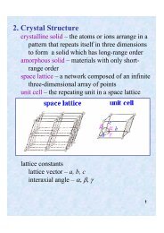


![Hetero [6+3] Cycloaddition of Fulvenes with N-Alkylidene Glycine ...](https://img.yumpu.com/35423358/1/190x245/hetero-6-3-cycloaddition-of-fulvenes-with-n-alkylidene-glycine-.jpg?quality=85)