PDF Viewing archiving 300 dpi - NHV.nu

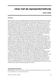
C, J, HEMKER
Elandsgracht 83
AMSTERDAM
COMMISSIE VOOR HYDROLOGISCH ONDERZOEK TNO
COMMITTEE FOR HYDROLOGICAL RESEARCH TNO
Verslagen en Mededeliilgen No. 23
Proceedings and I~~formations No. 23
PRECIPITATION AND MEASUREMENTS
OF PRECIPITATION
PROCEEDING OF
TECHNICAL MEETING 33
(April 1976)
VERSL. MEDED. COMM. HYDROL. ONDERZ. TNO 23 -THE HAGUE - 1977

PRECIPITATION AND MEASUREMENTS OF PRECIPITATION
COPY RIGHTS @ BY CENTRAL ORGANIZATION FOR APPLIED SCIENTIFIC
RESEARCH IN THE NETHERLANDS TNO 1977

ORIGIN OF PRECIPITATION
F.H. SCHMIDT
Royal Netherlands Meteorological Institute, De Bilt
In Western Europe, precipitation is normal phenomenon; it is of importance to
all aspects of society, particularly to agriculture, in cattle breeding and, of course, it is a
subject of hydrological research. Precipitation is an essential part in the hydrological
---,-- --- - *-
a&. How disastrous local conditions may be when precipitation holds off was obvious
recently in the Sahel territory, where for several years precipitation, which had previously
been marginal, stayed well under normally expected quantities. This introductory paper
aims at conclusions that may be drawn with respect to the distribution of rainfall, when
judged from a scrutiny of the mechanism that is responsible for the very origin of precipitation.
(See Fletcher (1 962) and Mason (197 1)).
Precipitation is exclusively caused by clouds, and the origin of clouds is in itself some-
thing special. The condensation of water vapour, which results into clouds, cannot take
w-rV=.% P
place in pure air. For, -- relative humidities of 300 to 40W0 would then be necessary and
-"*-+-.- --
such --...high .-. "L-e humiditiesnc~r
- -,"- occurin the-atmosphere. That is why condensation of water
vapour in the free atmosphere always takes place on small particles, the so-called condensation
nuclei. These condensation nuclei can have different dimensions, generally in the
order of l(rl to lop. It is interesting to note that larger condensation nuclei generally
lead to larger cloud-drops.
Condensation of water vapour generally takes place in the form of
these drops have temperatures below zero degrees centigrade, ice-crystals may be formed.
Generally speaking, in the free atmosphere this does not happen immediately at a temperature
of 0°C but as a rule at lower temperatures. Even at temperatures down to -10 or
-20"~ or, in extreme cases, even -40°C, waterdrops can still exist as such. They are
called super-cooled droplets. .-
For the forming of ice-crystals it is generally that small crystalline particles are present
in the waterdrops; around these crystalline particles, the waterdrops start freezing. So
there are clouds consisting of waterdrops only. There are also clouds at higher levels that
exclusively consist of ice-crystals. Very important for the genesis of precipitation are
those clouds that largely consist of waterdrops but in which ice-crystals are present too.
also peculiar. For there are clouds that do not give precipitation and others that do. This
means that apparently something special must be the matter with a cloud, should it
discharge in terms of rain, hail, or snow.

That such a special thing has to happen, becomes clear when the dimensions of cloud
particles are compared with those of precipitation drops. A normal cloud drop has a
diameter in the order of
--
10 to 100 micron. On the other hand, a normal rain drop has
dimensions of 1 to 6 mm. This means that, as its volume is proportional to its radius to
the third power, one thousand to one million cloud drops should coagulate to form just
one element of precipitation. It is clearly out of the question that a million or even one
thousand cloud drops present in a cloud, should in some way or other, without any
obvious cause, unite to one precipitation drop.
It has been proved that the origin of precipitation can only be explained when, in a
cloud, particles of various dimensions -are present. The larger particles in such a cloud,
having a higher rate of fall than the smaller particles, will fall, with regard to the latter,
and thus overtake them. It has also been proved that, in this way, such a large falling
cloud element can catch so many small cloud elements that the former at last gets
dimensions that correspond with the dimensions of a normal raindrop.
~~mulonimbi, observed during 7 test flights with a Fokker
Friendship. Numbers of flights are indicated. Number 564 refers to the flight over Amsterdam.
Numbers between brackets give estimated surface windspeed in knots. (From F.H. Schmidt in
Geofisica Pura e Applicata, 50,176,196 1).

CONTENTS
I. Origin of precipitation, F. H. SCHMIDT ..............................
11. The accuracy of measuring precipitation with a rain gauge network, H. A. R. DE BRUIN ...
111. The principles of measurement of precipitation with radar: a short introduction, H. A. R.
DEBRUIN ..............................................
IV. Areal precipitation measured by radar, W. ATTMANNSPACHER ...............
V. Measurement of rainfall by radar in the United Kingdom, T. W. HARROLD .........
VI. Is weather radar relevant to Dutch circumstances D. A. KRAIJENHOFF VAN DE LEUR .

AUTHORS
Prof.dr. F.H. SCHMIDT
Drs. H.A.R. DE BRUIN
Dr. W. ATTMANNSPACHER
Dr. T. W. HARROLD
Prof.11. D.A. KRAIJENHOFF
VAN DE LEUR
Royal Netherlands Meteorological Institute, De Bilt
Royal Netherlands Meteorological Institute, De Bilt
Deutscher Wetterdienst, Meteorological Observatory at
Hohenpeissenberg, FRG
Meteorological Office, Bracknell, U.K.
Agricultural University, Wageningen

Now another difficulty remains in that the question should be answered: how do such
large particles originate in a cloud In the first place this may be due t when ,$
id'
there is more or less strong turbulence in the cloud. However, as a rule this process leads
to no more than the relatively small droplets that occur in a drizzle.
To come to real precipitation, i.e. real rain or real snow, nature has two important
processes at its disposal. It has already been mentioned that condensation nuclei of differ- '"
s t dimensions can be present in the atmosphere and that the larger condensation nuclei
generally lead to the occurrence of larger drops. Here one finds a first possibility for large
particles to be originated in a cloud. These large particles fall, with regard to the smaller
ones, coagulation takes place and precipitation drops are formed. This process mainly
el
0 "C -T
2. Water vapour pressure as a function of temperature.
e = vapour pressure;
E = maximum vapour pressure for temperatures above freezing-point;
E, = maximum vapour pressure for vapour in contact with supercooled water;
Ei = maximum vapour pressure for vapour in contact with ice;
T = temperature.

takes place when&uffic@nt large condensation
---
nuclei --- are present, and that is generally the
------- - - ---
case - above seas.
hygroscopicity,
--
due to such large nuclei is a rather normal phenomenon. Also at moderate latitudes do
.sea-salt nuclei occur. This has been evident from measurements made during testflights of
a Fokker Friendship. It was then found that - above land, and - espzixi_ally over the city of
Amsterdam, a great number of small condensation nuclei and, therefore smaller droplets,
"-----. - -""------ -
were present in the clouds, whereas above the North Sea also large drops were observed to
occur in the clouds examined. (Fig. 1).
fir-weather eumull Cu 1 -- - - -
Cumulw congeatur Cu 2
.4ltostratur An ----
Simbtlrtur Ss ----
I .i M 25
3. Droplet spectrum in some cloud families.
Precipitating clouds are:
altostratus
nimbostratus
stratus (drizzle)
Non-precipitating are:
fair-weather cumuli
" stratocumulus.
6 Cumulus congestus may develop into precipitating cumulonimbus.
(from Mason, 1971)
3

Generally, another process is of much greater importance at moderate and high latitudes.
It _was already mentioned that, besides waterdrops, also ice->rystals appear in many
clouds. Now the maximum pressure of water vapour in contact with ice is lower than the
one when the water vapour is in contact with a supercooled water surface (Fig. 2). When
in a cloud, a so-called mixed cloud, besides waterdrops also ice-crystals are present, the
vapour press';;^re in the immediate surroundings of the crystals will be lower than the
vapour pressure in the immediate surroundings of the water-droplets. This results into a
vapour transport from places with - a high vapour pressure to places with a low pressure,
that is to say from the environment of the waterdrops to the environment of the icecrystals.
The vapour pressure around the waterdrops now becomes too low; the waterdrops
partly evaporate while the pressure around the ice-crystals becomes too high.
Higher, at least, than the maximum pressure that belongs to an ice-surface at the prevailing
temperature. This means that the ice-crystals will grow because vapour will condense
on them. And the -large -- crystals start falling with respect to still smaller ones and small
waterdrops. They will overtake these and grow by coagulation. In due course they will
continue their fall as snow-crystals or snowflakes. T&s process notably takes place at
moderate -.-"..."-". and high latitudes, which means that precipitation in these latitudes then
*-----
generally
-c*--- originates
e
.--,*we as snow. .* - Figure 3 shows the distribution of droplet radii in some
precipitating and non-precipitating clouds.
When temperatures between the level where the snow is formed and the ground remain
below freezing-point everywhere, snow is maintained as such. When the temperature near
the surface of the earth, or the lower air-layers lies above the freezing-point, the snow will
melt and it will start raining. Everybody knows that, at temperatures close to the
freezing-point, e.g. +2" or +3"C, raindrops that fall on a windshield of a car may give the
impression of little spurts that can be interpreted as snow-crystals that just melted and
which essentially fall apart against that shield.
The two processes sketched above both entail on opportunity for rainmaking. The first
one is mainly of importance in the tropics, where the following procedure is sometimes
applied. When a cloud does not show any tendency of giving precipitation, a quantity of
salt is brought into it, for instance by means of a balloon. Explosives next cause that salt
to be fragmented into small crystals. Being highly hygroscopical, these salt-crystals, when
diffused thr~ugh the cloud, cause the forming of large drops. These large drops, overtaking
the small ones, cause precipitation.
At temperature latitudes, precipitation can be generated when a cloud is available $&
temperatures below zero degrees centigrade in its upper parts, in which the amount of
ice-crystals, necessary to cause appreciable precipitation, is insufficient.
Particles are then brought into that cloud that have a crystal structure so much
resembling the structure of ice-crystals that the waterdrops contacting these crystals,
freeze. A well-known crystal used in this process is silveriodide. One can also decrease
temperatures in a cloud to about -60 or -70°C, by letting liquid C02 escape; in such

low temperatures waterdrops cannot maintain themselves in the atmosphere and generally
a sufficient number of ice-crystals will be formed to cause precipitation in that way.
The vital point in measuring precipitation is the question to what degree the intensity
of precipitation will difffer from place to place. It may be clear from the above that one
cannot expect precipitation to be equally heavy in all places.
In fact there may be more ice-crystals in one place than in others. Besides, for various
reasons, the number as well as the diameters of the waterdrops in a cloud are highly
# - p,
- - --
dependent on the upward movements in the cloud. This may be accounted for as follows:
from the same quantity of vapour in the air, the amount
be larger. It means that also more ----------- or larger drops --. will then come into existence than in a
.*
situation when the upward velocities in the air are lower. In the tests of the Fokker
Friendship, which we mentioned, the number of drops varied between 50 and 350 per
Diameter (mm)
4. The variation of drop diameter for range of updraught velocities according to Bowen. (from Mason,
1971)

em3 for the 7 flights, while the number of drops with a diameter of 50 pm varied from
1.79 to 0.03 per cm3.
itation is related to the upw& velocities - ~
he updraught, the longer the larger cloud
---"--
e&nts~~eg~@inthelg~&~ and they then have an opportunity to overtake more
small particles (Fig.4). In this way one can expect that clouds in which a strong upward
motion takes place, e.g. cumulonumbi, will generally give more precipitation than clouds
with weak upward currents like the layerclouds that form along warm fronts. As a matter
of fact, the velocities at which - the precipitating clouds pass the observation-place is $so
p---LIII-XIUI)LII -I^--.*(* ..
o_f__@portance. But, also within the cumulonimbus, the upward movement in one place
will be stronger than in another place; even in such apparently even clouds as warm-front
clouds, a stronger upward velocity will be present in one place than in an other. It means
that in both situations more precipitation will fall in one place than in another place, and
such precipitation differences may be present at rather short distances. To get a good
impression of the precipitation distribution in a certain area, one must therefore use a
great number of pluviometers.
Up to now there has been some talk of an accidental distribution of vertical speeds,
leading to an accidental distribution of water quantities in a cloud, and it is difficult to
find a conclusive explanation for this phenomenon. But there are other causes of precipi-
': ' '
5. The effect of the city of Rotterdam on the amount of precipitation during NE-ly winds in summer. ;-._--
Numbers are normalized as follows: (precipitation - average precipitation over the region): standard .
deviation. Examples: Rotterdam, station at the Westerkade average 9.4 mm, regional average 8,9
mm, lowest value at Zandvoort, at the coast, west of Amsterdam 5.5.
6. The effect of the city of Rotterdam on the amount of precipitation during SW-ly winds in winter.
Normalization as in Figure 5. Precipitation between 5 and 10 mm. Figures 5 and 6 are based on an
an investigation by Mr. G. J. Yperlaan.

A
tation differences that can be understood, as will now be shown with reference to some
relevant examples.
of big cities than at
7 ---m."l^I
the windward side; this can be understood with the help of the preceding reasoning. A
city is a +y~=of~h,e$t and, as a result, an upward movement of the air above the city
arises. An upward movement that moreover is intensifed due to the Lqer%~ou@ness in
the city compared with the surrounding area, which forces the horizontal air current
(the wind) to evade upward. So one might expect that at the leeward side of a city, m_o~
~aJgr"wil1 be present in the clouds than at the windward side; as a rule more precipitation
will then fall at the leeward side of a city. One can even find this on some charts of the
Climatological Atlas of the Netherlands. Recent investigations have also shown that there
are slight differences in the quantities of precipitation; this can partially be explained by the
effect of cities and large industrial areas (Figs. 5 and 6).
es like woods and hills also ca
ents of air and,
along with them a strengthening of the precipitation. Some investigators are convinced of
the existence of a wave motion perpendicular to lines along which
ness changes more or less abruptly
he effect of such a wave motion,
characterized by very weak upward
otions, seems to be present in the
precipitation pattern in the Netherlands (Fig. 7). How strong - - precipitation - can differ
from place to place during showery weather, appears from the total amounts when cold
WlNDDlRECTlON W-N
7. Possible effect of a weak wave motion, east of the coastline, on precipitation in the Netherlands
(from Timmerman, 1963).

air penetrates the Netherlands from the south, putting an end to a hot summer period.
It is during such invasions of cold air that most precipitation falls in this country. Figure
8 shows how strongly this precipitation can differ from place to place.
8. Precipitation in mm between 18 July 1964,7.40 gmt. and 19 July 1964,7.40 gmt., due to passage
of a cold front after a period of hot summer weather in the Nethe~lands. (hagel = hail; regen = rain).
(from H. R. A. Wessels, 1965).

An irregular precipitation pattern is often found along weak warm fronts. In such
situations it even happens that no precipitation is falling at all.
All in all it-seems that eve* a flat country like. the Netherlands,with only few natural
obstacles, -------- the distrjbution - -. of prec&i~on-_ma~bge~pjte irregular. Some aspects of this
irregularity appear on climatological maps. This means that, certainly for every day or for
every period of one hour or a few hours, the differences from place to place will be large.
Consequently, if one wants to have, for all kinds of purposes, an accurate impression of
the amount of precipitation that falls in small areas, special measurements should be
made to obtain sufficiently reliable results.
REFERENCES
FLETCHER, N.H. (1962) - The Physics of Rainclouds.
MASON, B. J. (1971) - The Physics of Clouds.
TIMMERMAN, H. (1963) - Mededelingen en Verhandelingen, No. 80, KNMI, De Bilt.
WESSELS, H. R.A. (1965) - Het noodweer van 18 juli 1964. Heme1 en Dampkring, 63, pp. 132-139.
INTRODUCTORY LITERATURE
MASON, B. 3. (1975) - Clouds, Rain and Rainmaking.
ROGERS, R. R. (1976) - A short course in Cloud Physics.
SCHMIDT, F. H. (1976) - Inleiding tot de Meteorologie, Aula 112.

THE ACCURACY OF MEASURING AREAL PRECIPITATION
WITH A RAIN GAUGE NETWORK
H. A. R. DE BRUIN
Royal Netherlands Meteorological Institute. De Bilt
1. SYNOPSIS
The main purpose of this technical meeting of the Committee for Hydrological
Research TNO, is to report on the use of radar for precipitation measurements. In
practice, areal precipitation is at the moment mainly determined by rain-gauge measurements
at individual points. The aim of this paper is to discuss the accuracy which this
method may yield.
Firstly, the instrumental errors of a rain-gauge proper are described. Secondly, the
spatial variability of a precipitation field is discussed. Thirdly, a theoretical approach of
the problem is given and, lastly, some results are shown of experiments carried out with
a relatively dense network of rain-gauges.
2. INTRODUCTION
For many hydrological applications, information on the precipitation depth averaged
over a certain area, S, and fallen in a certain time interval, T, is desirable. In practice, this
average is mostly determined with rain-gauge measurements taken at a finite number of
individual points.
It is perhaps interesting to relate that this method was first described many centuries
ago; Biswas (1971) reports that the Chinese scientist Chiu Chiu Shao, who lived about
1200 A.D., discussed it in his book "Shu Shu Chiu Chang".
The accuracy of the method depends on several factors. The instrumental accuracy is,
of course, important; the spatial statistical structure of a precipitation field, depending on
the climatological characteristics of the area of interest, plays a prominent part, while
further the quantities S, T, the number of rain-gauges, N, the spatial distribution of the
gauges, and the method of estimation itself may affect the accuracy of the method.
3. INSTRUMENTAL ERRORS OF A RAIN GAUGE
General remarks
A rain gauge is an instrument that has been used for thousands of years (Biswas,

1971). It usually has the form of a collector above a funnel leading into a receiver.
In the Netherlands, the so-called "national standard rain gauge" is installed with its
rim 40 cm above ground level, while since 1962 its orifice has an area of 200 cm2.
(Before 1962, its area was 400 cm2 and before 1946 its height 1.50 m).
In general, the catch of this rain gauge differs from the true precipitation depth
because of instrumental and observational errors. Some of these are discussed in the
following sections.
Systematic errors
A rain gauge is affected by a number of systematic errors. For instance:
and wetting losses; rain can splash in and out, and wind also acts on the gauge. Although
these errors depend on such factors as the nature of the gauge, the meteorological conditions
and characteristics of the site, Kurtyka (1953) (see also Rodda (1971)) has made the
following approximations (see Table 1) of the magnitude of the most important systematic
measuring faults:
Table 1
Evaporation Adhesion Colour Inclination Splash Wind and exposure
- 1 .O% -0.5% -0.5% -0.5% +1% -5 to -80%
It will be seen from this table that, except for the error caused by splash, the effects
are all negative, while the error due to wind and exposure appears to be the most irnportant.
Therefore, this error will now be discussed in more detail.
The process of wind acting on a rain gauge is rather complicated. Qualitatively it can
be described as follows:
Wind interacts with the gauge and the feature of the site to produce eddies and turbulence
in such a way that, in the region immediately above the gauge, raindrops or snowflakes
are accelerated. This results in an alteration of their trajectories by which a fraction
of the drops or flakes, which otherwise would have reached the orifice without disturbance,
is not caught by the gauge.
In Figure 1, taken from Green and Helliwell(1972), streamlines are drawn as measured
above a rain gauge installed in a steady wind flow of about 3 mls produced in a wind
tunnel. It is immediately noticeable that the effect of the rain-gauge is to cause a convergence
of streamlines from the windward edge of the gauge. The alteration of raindrop
trajectories is due to this convergence. Obviously, the trajectories . of small raindrops are
AT < . -
. .--*.A
-*-.\-%a .. \
3

AIRFLOW
TUNNEL W/S
3.05 mlsec.
10 crn
Fig. I. Streamlines above the Mk 2 raingauge funnel with a wind speed of 3.05 m/s, taken from
Green et. al. (1972).
, while a much greater proportion of snowflakes is
being deviated because of their larger surface area and their lower fall-velocities.
The results shown in Figure 1 are valid for steady wind flows. In natural field conditions,
the flow will be far from steady: it will be more gusty. Furthermore, the wind flow
is influenced by obstructions, such as bushes, in the vicinity of the raingauge. All these
factors together make that a quantitative description of the process is hardly possible.
In practice, the order of magnitude of the error due to the wind, as far as liquid
precipitation is concerned, is obtained by comparing the catch of the rain gauge of
interest with that of a so-called "pit gauge". This is a rain gauge installed in such a way
that its rim is at ground level. Usually an anti-splash grid is constructed to protect the
pit gauge against splash.
It is generally accepted that a pit gauge is not affected by wind. In the Netherlands, a
number of comparisons between the national standard rain gauge and a pit gauge was
carried out (see e.g. Braak (1945), Dey (1968), Colenbrander and St01 (1970)).

C II
% de bilt sleen
eibergen
Fig. 2. Seasonal fluctuation of the difference in precipitation depth between the standard rain gauge,
h,, and an international reference pit gauge, hp (0-o-o), and the seasonal fluctuation of the
mean wind speed (x-x-x); hp= 100%.
In Figure 2, the result of such comparisons made in 1972-1975 within the framework
of an international comparison programme, organized by the World Meteorological Organization
through its Commission for Instrumentation and Methods of Observation, are
given for the Dutch stations De Bilt, Eibergen (Hupsel) and Noord Sleen. It is seen that
in winter the pit gauge catches 6-8 per cent and in summer about 3 per cent more than
the national standard gauge.
4. RANDOM ERRORS OF A RAIN GAUGE
Random errors due to reading the measuringglass
In the Netherlands, the measuring glass is read to 0.1 mm. The average daily rainfall
amount is about 4 mm, if only wet days are taken into account. So the random error due
to reading the measuringglass is about 2.5 per cent of the average daily precipitation depth.
As about 50 per cent of the days are dry, the random error of monthly totals due to this
effect can be estimated with an accuracy better then 1 per cent.
Errors due to the 'kandom character of rain"
Let us imagine a cloud which procedures raindrops, so that the dropsize distribution
and the rainfall intensity do not vary with time. During fixed time intervals, T, we take
samples of the rainfall depth, h. If Ni is the number of raindrops caught during the i*
sample, we can write:

where !E3)i is the average value of the third power of the diameter of the raindrops
caught during the ith sample, and 0 the area of the rain gauge. Doing so, it will be
observed that in general the values of hl, ha, h,, ... are not equal. This variation is
caused by random variation in N and E3, due to sampling effects. Appendix I shows,
that the relative value of the random error caused by this effect is given by:
It should be noted that N is proportional to 0, so o(h)/h m c
During 1968 and the first few months of 1969, raindrop-size measurements were
carried out at De Bilt, using a filter-paper technique (Wessels, 1972). These data (one
purpose to collect them was to determine the relationship between rainfall rate and radar
reflectivity) were used to get an impression of the order of magnitude of o(h)/f;. It should
be remarked that the measurements could only be carried out in working time. Table 2
shows some results for "daily" rainfall amounts and for two values of 0 (20 and 200cm2).
Table 2
0 = 20 cm2 0 = 200 cm2
-
date h mm o(h)/i;. 100 a(h)/f;. 100 N(0 = 20 cm2)

Table 3 shows some examples of short time intervals:
Table 3
AT min
From these tables it can be concluded that the error due to random character of
rain is negligible for rain gauges having an area of 200 cm2.
In the literature (see for instance Kalma et al. 1969), rain gauges with smaller areas are
described. It is seen from Tables 2 and 3 that for these types of gauges the values of
a (h j/f; are not negligible.
.,%"- *"--
I-M ++a -"
Fig. 3. Spatial distribution of daily precipitation amounts, as measured in Salland on May 24, 1972,
with the national rain gauge network (Fig. 3a) and a dense network (Fig. 3b).

5. SPATIAL VARIABILITY WITHIN A PRECIPITATION FIELD
From our own experiences we know that the spatial distribution of precipitation can
be highly irregular. The meteorological processes responsible for this variability were
reviewed this morning by Schmidt (1976).
To illustrate the possible differences over a short distance, the spatial distribution of
the daily precipitation amounts is shown in Figure 3, as measured on May 24, 1972, with
a dense network installed in Salland, a district in the eastern part of the Netherlands, in
1970-1972. This was done within the framework of a hydrological research programme
(Santing et al., 1974).
In this figure the same precipitation field is drawn as "seen" by the (less denser)
national rain gauge network of the Royal Netherlands Meteorological Institute.
This example shows that, over distances of 1 kilometre, differences of 20 mm/day can
occur.
Generally, these differences within areas such as Salland are not systematic. For most
of the practical applications, areas in the Netherlands of, say, 1000 krn2 can largely be
considered to be climatologically homogeneous and isotrope.
It will be pointed out in the next section that a convenient quantity to describe the
statistical spatial structure of a precipitation field is the correlation coefficient, p, defined
by:
in which the bars indicate an average over a long time series; hi and hk are the precipitation
depth measured at the ith and kth station, while oi and ok are the standard deviations
(of time series) of these stations.
If the distance between the two stations is denoted by rik, it is to be expected that
pik decreases with increasing rik, if a homogeneous and isotrope area is considered.
It has been found (see e.g. St01 (1972) and De Bruin, (1975) that the "correlation
function", p(r), can be (more or less) satisfactorily described by:
which relationship can be written for r

100 x correlatie coefficient
100,
Fig. 4. The correlation coefficient, p, as a function of the distance, r, for each month (daily totals),
taken from St01 (1967).
Table 4
month po ro km
1 .97 962
2 .96 630
3 .95 320
4 .94 190
5 .93 135
6 .9 1 111
7 .9 1 104
8 .92 110
9 .93 133
10 .95 186
11 .96 309
12 .97 609
Year .94 188

Ten days total from 36 stations in the same area and of the period 1966-1972, were
processed by De Bruin (1975). He concluded that for r, up to about 30 km, equation (5)
can be used. However, he found a big scatter plotting p against r (a scatter which, after
all, is also present in the data of Stol). De Bruin pointed out that this scatter is partly due
to random observational errors, because these lower the value of p and, therefore,
increase its variability.
Table 5 shows the values of po and ro from (S), as found by De Bruin for 14 selected
stations. Furthermore, the corresponding values of all 36 stations are listed.
Table 5
period
Nov.-March
Sept., Oct., Apr., May
July-Aug.
14 selected stations all 36 stations
PO rokm PO rokm
.99 1000 .95 1000
.99 270 .98 270
.99 190 .99 190
It is seen from Tables 4 and 5 that a seasonal effect exists: in winter, ro has a
maximum and in summer a minumum value. This is so because in winter mainly frontal
(that is large-scale) precipitation occurs, whereas in summer also convective storms (smallscale
precipitation) are likely to occur.
Table 6 lists the values of po and ro from equation (5) for 5-day periods and different
"seasons", as found in Salland by means of the records of the dense raingauge network
mentioned before. The values found in this network for 1 and 10-days periods were
similar to those listed in Tables 4 and 5.
Table 6
period
"year"
"summer"
selected stations
Po
ro km
.97 230
.97 150

6. ACCURACY OF THE ESTIMATES OF AREAL PRECIPITATION
Estimate with one rain gauge
A homogeneous, isotrope and square area, S, with edge II is considered. In the centre.
P, of this area, a rain gauge is installed.
The precipitation depth averaged over the area is denoted by hG, while that measured
at P is called ho. As the area is supposed to be homogeneous, an estimate of hG is:
A
hG = ho (6)
Appendix I1 shows that the standard error of this estimate, E, defined by E2 =
(hG-GG)', can be written as:
"I
E2 = u2 [(1 + 0.23 -
r 0
where u is the standard deviation of a long time series taken at an arbitrary point in S.
This relationship is valid, if equations (4) or (5) are supposed to be true.
Introducing Z = Elk and C, = u/K, we obtain:
Table 7 shows some characteristic values of C, for different time intervals.
Table 7
T days
C, = u/h
Accuracy obtained with N evenly distributed rain gauges
Next, the case is considered that N rain gauges are evenly distributed over area S. The
recorded precipitation depths at these stations are denoted by h, , h2 , ..., hN.

Fig. 50-5d.
The relative error, Z (%), as a function of SIN (km2) for the time intervals of lday (Sa),
5 days (5b), 10 days (5c) and 1 month (5d).

Fig. 5d

An estimate of hG is now given by:
while the relative error Z can be written as
(See Appendix 11, and also Kagan, 1972).
Figures 5a, b, c and d present Z drawn as a function of S/N for various values of S and
for different time intervals.
Some remarks on equation (1 0)
The reliability of equation (10) depends on the quantities po and ro, found with the
empirical correlation function given by (4) and (5). But, because of the rather big scatter
observed when correlation coefficient p is plotted against distance r, the accuracy of
these quantities (notably that of po) is not very high. This is one of the main problems of
this "theoretical" approach.
Quantity po has been introduced as a result of the random errors of observation (see
Appendix 11). Although po can be determined only with a relatively low accuracy, it is
interesting to see what happens when the value of po is altered.
In Figure 6, Z is drawn as a function of S/N for 1000 km2 and 10-day totals, while the
following values of po were chosen: 0.96,0.99 and 0.9973, corresponding with A = 0.20,
0.10 and 0.05 respectively (A is the random error of observation divided by a). Suppose
we have a rain-gauge network with SIN = 100 km2 and A = 0.20. It is then seen from
Figure 6 that in a network with S/N%230km2 and A = 0.10, or SIN = 320 krn2 and
A = 0.05, the same value of Z is obtained. This example is given to illustrate that under
certain circumstances it can be more economical to decrease the number of rain gauges,
if at the same time the random measuring error is lowered (for instance, by means of
automation of the network).
7. COMPARISONS WITH A DENSE NETWORK IN SALLAND AND IN ZUID-HOLLAND
It is in itself a problem to test the reliability of equation (10). The only thing one can
do is compare the records of a dense and a less dense network of rain-gauges with one
another, assuming that the densest network gives the true areal precipitation depth.
In this manner, the data of a network of rain gauges installed in Salland during 1970-
1972 were used.

Fig. 6. The relative error, Z (%I, as a function of SIN (km2) for different values of p, (lodays
period and S = 1000 km2).

Within an area of about 1100 km2, rain gauges were erected at 65 points. These are
plotted in Figure 7. It is seen that in principle the gauges are evenly distributed over the
area. They form a 5 x 5 km grid. In the centre of the area (in the neighbourhood of
Heeten), the network had a special density.
8 -
''7'
J
Lenele
Fig. 7.
The dense network of rain gauges in Salland.

Here the distances between two stations were up to about 750 m. In order to avoid the
systematic measuring error due to wind, pit gauges were used. For budgetary and organizing
reasons, a special, cheap type was developed; see Figure 8.
Fig. 8. Schematic crosssection
of the
'Salland pit-gauge'

Comparisons between this type of rain gauge and an international standard pit gauge,
mentioned in one of the previous sections, were carried out at De Bilt in 1972-1975.
Two "international" pit gauges were installed next to three "Salland" pit gauges.
salland
pit
J
I I I
I I I I I I I I I I I
0 50 100 150
Fig. 9. Comparison between the monthly precipitation depth measured at De Bilt with the ''Salland
pit-gauge" and the international reference pitgauge (mm).
In Figure 9, the means of the monthly totals measured with the three "Salland" gauges are
plotted against those of .the two "international" gauges. It is seen that there are hardly
any differences between the two types of pit gauges. (De Bruin, 1973).
Unfortunately, it appeared that the daily records of about 30% of the stations were
inadequate (Yperlaan, 1974), so only the data of 42 stations could be used for testing
equation (10) as far as daily totals were considered. For lO-day totals all 65 stations were

Figs. 10-12. Comparison between theoretical and experimental values of Z (%) as found, with a
dense network of rain gauges in Salland for:
an area of = 1000 km2 and a time interval of 10 days (Fig. 10);
an area of = 1000 km2 and 1 day (Fig. 11);
and = 1 and = 100 km2 and 1 day (Fig. 12).

used. The arithmetic means of the records of these data were taken as the true areal
precipitation depth.
The areal precipitation depths of 72 10-day periods were estimated with 1, 2 and 5
stations of the national rain gauge network, respectively, each covering about 1000,500
and 200 km2, respectively. As the five stations were not evenly distributed over the area,
the "Thiessen average" was taken as an estimate. These estimates were compared with the
"true" precipitation depth obtained with the dense network. The respective values of Z
were calculated; they are plotted in Figure 10. In this figure, also the theoretical line
given by equation (10) is drawn. It is seen that there is fairly good agreement between
experimental and theoretical values of Z. It can be shown that (10) underestimates Z, if
the stations are not evenly distributed. This explains the rather big deviation of the experimental
2-value for S/N = 200 km2.
The same procedure was followed for daily totals. The results for 1000, 100 and
1 km2 are given in Figures 11 and 12. Again, there is agreement although with a tendency
that (1 0) underestimates 2.
Unfortunately, the procedure under consideration only gives a few examples for
testing equation (10); it is, therefore, dangerous to draw definite conclusions.
Finally, similar experiments are being considered, carried out by Kruizinga and Yperlaan,
1976 with the records of 35 stations situated in the province of Zuid Holland, in the
western part of the Netherlands. The total area was about 4000 km2.
The mean daily precipitation depth over this area was estimated with the daily records
of 4 stations, and the average over a sub-area of about 400 km2 was estimated with the
measurements at 1, 3 and 4 points, respectively. In the case of four points, the stations
were situated outside the area.
Kruizinga and Yperlaan did not use quantity Z as a measure of error of estimate. They
took the mean of the absolute value of the differences between the estimate and the true
areal rainfall depth. So, in the first instance, their results are not comparable with
equation (10). However, experiments with the records of the "Salland network" reveal
that the "mean absolute difference" error is about 0.5 times the "root mean square"
error, from which Z is derived. This is partly due to the sensitiveness of Z to outliers.
Using this conversion factor, we plotted the results of Kruizinga and Yperlaan in
Figure 13, where also the theoretical lines for 400 and 4000 km2
It should be noted that Kruizinga and Yperlaan described the error of estimates as a
function of the "true" areal rainfall depth and the four seasons, while dry days were also
concerned. The values given in Figure 13 are recalculated for rainy days. No distinction
is made between the rainfall depth and the seasons.
Again, it can be concluded that equation (10) fits fairly well to the experimental
values of Z. However, we should bear in mind that the experimental values of Z for this
example were obtained in a rather crude way.
ACKNOWLEDGEMENT
The author is greatly indebted to Mr. S. Kruizinga for valuable advice.

REFERENCES
BISWAS, A.K. (1971) - History of Hydrology. Amsterdam etc. North-Holland Publ. Comp.
BRAAK, C. (1945) - Invloed van wind op regenwaarnemingen. KNMI Med. en Verh. 48 De Bilt,
Staatsuitgeverij '~Gravenhage, (English summary).
DE BRUIN, H.A.R. (1973) - Gegevens betreffende neerslag en verdamping verzameld in Salland gedurende
1970-1972 ten behoeve van de Werkgroep Hydrologisch Onderzoek Overijssel. KNMI
W.R. 734, De Bilt. (English summary).
DE BRUIN, H.A.R. (1975) - Over het interpoleren van de neerslaghoogte. KNMI W.R. 75-2, De Bilt,
(English summary).
COLENBRANDER, H.J. and Ph.Th. STOL (1970) - Neerslagverdeling naar plaats en tijd. Tweede
interimrapport Werkgroep I van de Com. ter Bestudering van de Waterbehoefte van de Gelderse
Landbouwgronden. Deelrapport 5, pp. 89-108. (English summary).
DEY, L.J.L. (1968) - Enige opmerkingen over de neerslagmeting en de neerslagverdeling naar tijd en
plaats in ons land. Versl. en Med. No. 14 Com. v. Hydr. Ond. TNO, Den Haag, pp. 71-85.
English summary).
GREEN, M.J. and P.R. HELLIWELL (1972) - The effect of wind on the rainfall catch. Symposium
on Distribution of precipitation in mountainous areas. Geilo, Norway, 31-715-8-1972, WMO
NO. 326, Vol I1 pp. 27-47.
KAGAN, R.L. (1972) - Planning the spatial distribution of hydrological stations to meet an error
criterion. Casebook on hydrological network design practice 111. 1.2, WMO No. 324, Geneva.
KALMA, J.D., J. LOMAS, M. THALLER, and Y. SHASHONA (1969) - An accurate small orifice
rain-gauge. Wat. Res. Res.; 5, (1969), No. 3, pp. 300-305.
KRUIZINGA, S., and G.J. YPERLAAN (1976) - Ruimtelijke interpolatie van dagtotalen van de neerslag.
Een experimentele benadering. KNMI W.R. 764, De Bilt. (English summary).
KURTYKA, J.C. (1953) - Precipitation measurements study. Report of investigation No. 20, State
Water Survey Illinois, pp. 178.
RODDA, J.C. (1971) - The precipitation measurement paradox - the instrumental problem. Reports
on WMOIIHD projects No. 16, World Meteorological Organization, Geneva.
SANTING, G. et al. (1974) - The hydrological investigation programme in Salland (Netherlands).
Versl. en Med. No. 19 Com. v. Hydr. Ond. TNO, Den Haag.
SCHMIDT, F. H. (1977) - The origin of precipitation. Versl. en Med.; No. 23 Com. v. Hydr. Ond.
TNO, Den Haag.
STOL, Ph.Th. (1976) - Dagefijks neerslaghoeveelheden in de Gelderse Achterhoek in verband gebracht
met de onderlinge afstand van de plaats van meting. I.C.W. Wageningen Note 426.
STOL, Ph.Th. (1972) - The relative efficiency of the density of rain-gauge networks. J. Hydrol. 15,
pp. 193-208.
WESSELS, H.R.A. (1972) - Metingen van regendruppels. KNMI W.R. 72-6 De Bilt (English summary).
YPERLAAN, G.J. (1974) - Kwaliteitscontrole van de neerslagmetingen van het Hydrologisch Onderzoek
Overijssel. KNMI W.R. 74-10, De Bilt. (English summary).

APPENDIX I
ERRORS DUE TO THE "RANDOM CHARACTER OF RAIN"
When the precipitation depth, h, is measured with a rain gauge, a number of raindrops,
N, with different diameters is caught during a certain time, T.
If we were able to repeat the experiment, it would be expected that we would not find
the same number of drops and the same dropsize distribution. This indefiniteness in both
the number of drops and the size distribution springs from the random nature of the rainproducing
process.
We can write:
where g3 is the average value of the third power of the dropdiameters, and 0 is the area
of the orifice of the rain gauge. If we could repeat the measurement of h many times, we
would get the average value of h, N and E3, denoted by respectively h, fl and E3.
Our problem is to find the random fluctuations of h, N and E3 round their means.
A measure for these functions is the standard deviation a defined by:
- -
a2(x) = (x - j~)2 = x2 - ~2
-
First, we remark that it is reasonable to assume that the random fluctuations of N and
D3 are independent, so we can write for small a (N) and o (E3):
Further, we note that the standard deviation of the mean of P samples of a stochastic
variable is equal to the standard deviation of the variable itself, divided by t/~. SO we can
estimate a(E3) with
This results into:
3 2 1 3 -- I
( E m N
The problem to determine a (N) remains. We, therefore, divide the time interval, T,
into M equal time intervals, where M >> N. If it is assumed that two raindrops never

each the orifice simultaneously, which makes it possible to choose M in such a manner,
that never more than one drop is caught during an interval; the chance that during any
interval a raindrop is caught is N/M. The chance that during any given interval no drop is
caught is (I -N/M). It can then be proved that the probability that during N intervals a
raindrop is caught can be written as:
For large N, this equation transforms into:
This is the Poisson distribution, for which
o(N) = di
From (I.2), (1.3) and (1.6) we obtain:
If we have only 1 sample
0 ) -
--, is of course estimated with
h
APPENDIX I1
DERIVATION OF EQUATIONS (7) AND (10)
It is assumed that the region of interest is square-shaped and has an area S, while at its
centre, P, a rain gauge is installed. Let ho be the precipitation depth measured at P during
a certain time interval, T. The mean precipitation depth over S is denoted by hG.
Further, it is assumed that the area is climatologically homogeneous and isotrope.
Because of these assumptions, a reasonable estimate of hG will be:
Now let us imagine that S is covered by a dense and regular network of ideal rain
gauges. The precipitation depths obtained at these stations are denoted by h, h; ..., h:.

We can write:
In fact:
A measure of accuracy of the estimate given by equation (11.1) is the quantity defined
A
The bar denotes an average over a large series of hG and hG.
From equations (11. I), (11.2) and (II.3), we obtain:
N -
E2 = lim 2(hthf -htho -hrho +%)
N,,N~ i=1 j=l
The measured precipitation depth, ho, can be written as
where h,* is the true precipitation depth at P, and 6 is a random measuring error with
F= 0. (For the sake of simplicity it is assumed that ho has been corrected for systematic
errors such as those due to wind).
Further, it is reasonable to assume that:
The Quantity 62 is the standard error of observations at P.
From equations (II.4), (11.5) and (11.6) we get:
As the homogeneity of S has been assumed, we can write:
(i = 1, ... N).
w-m
Thus the correlation cozff$ent
pB=
"ioj

is equal to
-
h: hr - x2
p* =
U fJ2
So we obtain:
where
-
As we have seen, the correlation coefficient can be described by equation (4):
p (r) = po e-'Ir0
It is noted that this relationship has been found for the correlation coefficients
computed with the series of measured precipitation depths, while p; stands for the correlation
between two series of true precipitation.
If, analogously to (II.5), we write:
hi = h: +Gi, hi = h* +6
J j
then it can easily be shown that:
* 1
Pij = Pij -(i f j)
A2 + 1
If it is assumed that:
the "true" correlation function, p;, will reach the value 1 for r -+ O.*) Thus, combining
equations (4) and (II.13), we find:
and
1
Po =- A2 + 1
1
If A50.25, then -- x 1 -A2, so A2
o2 + 1
*) assuming that PO is indcpcndent of rij.
1 -po

46
Substituting (11.15) and (11.16) into (11.1 1) we get:
I N N
I
~2 = o2 [(1 + lim - Z e r i j i ~
N+- ~2 i=l i=l
- i - e-rj~ir~
+ 1
(11.1 7)
With the aid of a computer, the term
was determined for a square area S (see Kagan, 1972).
In this way
is obtained.
Next, we consider the situation that n rain gauges are evenly distributed over S. The
precipitation depths recorded at these points are denoted by h, , h2, ..., h,.
Each rain gauge covers a subarea S/n.
The areal precipitation depths of this subarea is now estimated with the precipitation
depth recorded at the station belonging to it.
That means that:
The standard error of estimation for the ith subarea is given by (11.18):
Assuming that the errors of estimate for the various subareas are independent, we can
write for the standard error of the estimate given by (11.19):

THE PRINCIPLES OF MEASUREMENT OF PRECIPITATION WITH RADAR:
A SHORT INTRODUCTION
H. A. R. DE BRUIN
Royal Netherlands Meteorological Institute, De Bilt
1. SYNOPSIS
It is to be expected that the technical meeting on radar measurements of precipitation
organized by the Committee for Hydrological Research TNO will be attended by hydrologists
and others concerned with water management and water supply, who are generally
not acquainted with the principles of radar and its application for precipitation measurements.
Therefore, the basic physical formulae and their background are briefly reviewed.
2. QUALITATIVE OUTLINE
Radar is based on the principle that an electromagnetic wave propagages along a
straight line through the atmosphere with a velocity equal to light speed (= 3.10' mls).
Objects such as raindrops will scatter and reflect electromagnetic energy. When an
instrument is constructed which is able to transmit an electromagnetic pulse and which
can also intercept reflected signals, one can measure the time interval between the transmission
of the pulse and the reception of the reflected signal and thus determine the
distance to the object. Measuring the intensity of the reflected pulse will yield information
of the object itself. Such an instrument is called 'radar', when it transmits radio
waves (with wavelengths of the order of cm -m).
antenna'
transmitter
1-1
receiver
automatic switch
data processing
system

Radar (see Fig. 1) essentially consists of a transmitter which produces the power at the
radio frequency, a parabolic antenna which radiates the power in a narrow beam, an antenna
which intercepts the reflected signals, a receiver which detects and amplifies the intercepted
signals, and an automatic switch to close the receiver during the short interval
when the transmitter is operating.
Finally, a radar is equiped with a system which processes the returned signals. Often a
cathode ray tube is used, together with an oscilloscope, to visualize the received power.
Today also computer systems are "interfaced" to the radar set.
It is noted that in practice a single antenna is used for both transmission and reception.
3. BACKSCATTERING OF A SINGLE SMALL SPHERICAL PRECIPITATION PARTICLE
Let Wo, Uo and h respectively be the power per unit area, the amplitude and the wavelength
of the transmitted radio wave. This wave is scattered in all directions by a spherical
precipitation particle at a distance r from the radar set and with a diameter D

This gives:
The intensity of the scattered wave intercepted by the antenna is proportional to Ug,
so we can write (as Ui - Wo):
where Wt, is the power per unit of area intercepted by the antenna. Equation (4) is the
well-known scattering law of Rayleigh.
4. BACKSCATTERING OF A NUMBER OF PARTICLES
When one uses radar for precipitation measurements, the radar beam illuminates a large
group of raindrops (snowflakes, hailstones, etc.). So the backscattering of a large number
of particles has to be considered. A radar pulse covers, during "pulse time" T, a distance
h (the "pulse length"). The power backscattered by particles at a range (r + h/2) from the
front of the pulse of length h arrives at the antenna, at the same time as the power backscattered
by particlesat a range r from the rear of the pulse. At a certain time t, the antenn02r2h
na receives signals from particles within a volume that is equal to about -(see
8
Fig. 2) where 6 is the "beam-width".
Assuming that the particles are distributed at random, the total power per unit of area
received by the antenna can be written as:
w 0
Wb -- f2 (N) 6' r2 h Z D:
r2 h4
VO~

where Z: Dt is the sum of the 6th power of the diameter of the particle within a unit
vol
of volurns. Z = Z: D; is oiian called the 'reflectivity factor'.
It has been f%nd that the backscattered signal varies from one reflected pulse to the
next. This is caused by movements of the particles with respect to one another. Therefore,
in practice the averaged power per unit of area Wb of a number of reflected pulses
is detected.
5. THE RADAR EQUATION
Until now the averaged reflected power per unit area Wb intercepted by the antenna
has been described as a function of Wo, the power per unit of area intercepted by the
scattering precipitation particles.
The power, Pt, transmitted by the radar set is concentrated in a narrow beam of width
0. Particles at a range r along the axis of this beam will receive a power per unit of area
W, , which is proportional to P,/O (see Fig. 3).
Obviously, 0 -- 8' r2. So we obtain, if the radar beam is entirely filled with precipitation
particles:
wo - ~ ~ / t ~ ~ r ~ (6)
Substituting (6) in (S), we can write:
The total average power, Fr, intercepted by the antenna is equal to qt, . A,, where Ae
is the effective area of the antenna. It is found that A, = 4 A (A is the actual area of the
antenna), if the antenna is circular.

This gives:
It can be shown that f2 (N)
N2-1
= -
1 N2 +21
It should be noted that f2(N) may be taken as 0.93 and 0.20 for water and ice particles,
respectively.
From (8) and (9) we obtain the "radar equation":
where C is a constant (which is about 50).
This equation can be written as:
where C1 is a parameter that depends on the characteristics of the radar set, and C2 is
related to the optical properties of the precipitation particles.
In the derivation of (1 1) no provision is made for attenuation caused by absorption
and scattering of precipitation present between radar and observed volume.
Some authors (e.g. Collier) introduce an attenuation factor K; (1 1) can then be written
as :
This factor is introduced to describe the effect of attenuation of precipitation that
occurs between the radar set and the observed volume.

6. SOME NUMERICAL EXAMPLES
In order to get an impression of the magnitude of the various quantities, Table 1 lists
some characteristic values.
Table 1
Quantity
transmitted power Pt
lo4-lo6 w
minimum detectable power Pmin 10-'~--10-'~ W
pulse time T 0.2- 4 s
pulse length h
60-1 200 m
beam width 6
0.5-2 deg.
wavelength h
0.03-0.1 m
Now it is supposed that we have a radar set with Pt = 2.105W, Pmi,=2.10-'3W,
A = 1.5 m2, ,h = 0.05 m and h = 900 m, while we observe spherical waterdrops at a
distance of 100 km.
Equation (10) can then be written as:
The backscattered power intercepted by the radar antenna will be detected only if
threshold value Pmin is crossed.
So the waterdrops are "seen", if:
z > 10-1' (m6 1m3 (14)
Typical values of drop sizes are 1 mm and 0.15 mm during rain and drizzle, respectively,
whereas cloud droplets have diameters in the order of 3.10-~ m.
So condition (14) is fulfilled if within 1 m3 at least 10 raindrops, 9.10' "drizzle
drops" or about 10'' cloud droplets are present. For rain and drizzle thcx values are
realistic, but the maximum concentration of cloud droplets is about lo8 per m3. So this
example shows that with radar rain and drizzle are detectable, whereas clouds are not
"seen".
7. SPECIAL PROBLEMS
Some factors limit the use of radar for precipitation measurements. We would mention
four:

A. Melting layer
In one of the previous sections it has been seen that water and ice have different
N2-1
optical properties, resulting in different values of 1-1 (0.93 and 0.20, respectively).
N2 +2
When a snowflake is melting, first a water-skin arises. At this stage, the flake is "seen"
by the radar as a waterdrop with the size of the snowflake. This causes an increase of the
radar echo. So, when the radar beam intersects the O"C layer, a "bright band" is observed.
This effect limits the accuracy of rainfall measurements.
B. Attenuation
It was noted before that rain present between the radar set and the volume of interest
will attenuate the power. Especially with heavy rainfall, this problem is serious.
C. Alteration of rainfall rate with height
Radar detects rain above ground level; so when the rainfall rate alters between the
radar beam and the ground, a wrong rainfall rate is observed.
D. Anomalous propagation
Under some atmospheric conditions, radio waves do not propagate along a straight
line.
8. RELATION BETWEEN Z AND PRECIPITATION RATE, R
The last step missing is the relation between Z and precipitation rate R. This relationship
depends on the shape of the distribution of the sizes of particles. This follows directly
from :
where ND is the number of drops per unit size range per unit volume of air in the class
AD whose average diameter is D, MD is the mass of the individual particles and uD is the
fall speed. (Obviously, MD = 2pD3, p is the density).
In the same way, Z can be written as:
D max
Z= I: N ~ D ~ A D
D=O

Marshall and Palmer (1 948) gave an approximation of ND :
where A is a constant.
With the approximation of Gunn and Kinzer (1 949) for the fall speed:
uo % 1 30a (1 8)
(D in metres, UD in m/s) we obtain, after elimination of A, if we take a typical value for
No = 107m-4:
(R in mmlhr).
This analysis is too crude. Therefore, in practice, the empirical relationship
Z=A- R~ (20)
is used.
The problem of this equation is the large variability of its parameters A and B.
Several authors (see e.g. Hitschfeld and Bordan (1954) and Collier (1975) have shown
that the accuracy of radar precipitation measurements will be improved if rain gauges are
used to calibrate parameters A and B. This is, for instance, achieved in the Dee Project
and in the experiments at Hohenpeissenberg. Both will be described during this meeting.
For more detailed information on the principles of radar, and its application for precipitation
measuring, readers are referred to Battan (1973) and Kessler and Wilk (1968).
REFERENCES
BATTAN, L.J. (1973) - Radar Observation of the Atmosphere. The University of Chicago Press,
Chicago.
COLLIER, C.G. (1975) - Rainfall Measurements by Radar. Symposium on Weather Radar and Water
management, Chester U.K.
GUNN, R. and G.D. KINSER (1949) - The terminal of fall for water droplets in stagnant air.
J. Meteorol. 6 (1949), no.4, pp. 243-248.
HITSCHFELD, W. and J. BORDAN (1954) - Errors inherent in the radar measurement of rainfall at
attenuating wavelengths. J. Meteorol. 2 (19541, no.1, pp. 58-67.
KESSLER, E. and K.E. WILK (1968) - Radar measurements of Precipitation for hydrological purposes.
WMO/IHD report no.5.
MARSHALL, J.S. and W.Mc. PALMER (1948) - The distribution of raindrops with size. J. Meteorol.
5 (1948), no.4, pp. 165-166.

AREAL PRECIPITATION MEASURED BY RADAR
W. ATTMANNSPACHER
Deutscher Wetterdienst, Meteorological Observatory at Hohenpeissenberg, FRG
1. INTRODUCTION
The measuring of precipitation seems to be the oldest meteorological facility on earth;
from the literature it is known that about 400 B.C. the first rain measurements were done
in India (Kautilya, 1915). About 2000 years later Wren built the first rain gauge in England
(PLeiss, 1969). Most of the rain gauges used in ~urope today were developed in the
1880's and 1890's (Hellmann, 1885 and Fuess, 1897). The necessity of higher accuracy
has led to new designs and constructions of rain gauges in recent years, for example the
Obrometer of Joss (1967) and that of the Observatory at Hohenpeissenberg (Attmannspacher,
1973). Such an instrument provides suitable knowledge on local precipitation in
terms of duration, amount and intensity at one point.
29.5.1968: rain shower
. . - - - - - - -
. . .
.- -.- .-
-- - .. .-
-. --
. -.. -... - --
--- .-..
--.
-
. .
17.5.1968 :,,steadyUrain
.- - - -- -
--- -- -- -
Fig. I: Minute precipitation intensities during a rainshower (upper part) and during "steady" rain;
Hohenpeissenberg, 1968.

An example of variation in precipitation intensities from minute to minute is shown
in Fig. 1. Within a shower, the precipitation intensity changes from minute to minute by
a factor of 10. For steady rain, the minute-to-minute differences reach a factor of 4. The
areal variations are at least of the same order as those of time. Single measurements at
one point, over a period of some years, will smooth the differences in time and area. But
for many specific questions in hydrology, knowledge of the true areal precipitation for
single cases is doubtless necessary. To be able to get sufficient knowledge of these areal
precipitations, a dense rain-gauge network may be useful. Else an other facility for areal
precipitation measurement will have to be found.
Fig. 2 shows the amount of precipitation in a dense rain-gauge network, which is
installed north of the Hohenpeissenberg, and the results of areal precipitation measurement
using radar. Even with the data of this dense network of about 50 rain-gauges
operating in an area of 750 km2, it is impossible to draw realistic isohyets; but they can
be drawn easily if radar measurement is practised.
As early as 1904, the German Patent Office granted a patent to an engineer, Huelsmeyer
(Brockhaus Lexikon, 1954) for a navigation instrument which received radio waves
being reflected from a ship. About 30 years later, this idea was used in systems for radio
navigation developed in several countries. Those systems were soon found to be disturbed
in situations of bad weather. Meteorologists next studied the unwanted echos and, finally,
radar became an important tool in meteorological science. For example, for measuring
areal precipitation. As the literature reveals, more than 20 years ago the first steps in this
field were taken by Americans (Battan, 1973) and Russians (Borovikov, 1967). Over the
last 10 years scientists in other countries also started much work on radar used for hydrological
measuring.
2. PRINCIPLE OF AREAL PRECIPITATION MEASUREMENT USING RADAR
The measuring of areal precipitation is a simple technique: a pulse of the radar equipment
is sent out and the echos coming back from the precipitation, that is from the raindrops,
are received and their intensity is measured. As long as the rain-drop diameters are
much smaller than the radar wavelength (Ralleigh Approximation) based in the Mie
Theory, the radar equation can be written as:

Jsohyets
= Radar Results
lOkm 10km 20km
Fig. 2: Radar- and rain gauge results; Hohenpeissenberg, 1.9.1970, 13.35-17.30 MET.

jii, = mean received power
Pt = transmitted peak power
h = pulse length
A, = effective aerial aperture
r = range
F = correction factor for partly filled radar volume
K = Correction factor for attenuation of radar power by the rain itself
a = equivalent back scattering cross-section of all drops in unit volume of the beam.
The factors in this equation are functions of the radar equipment; or of the objects
causing the echo, in other words: the raindrops.
To be able to get realistic measurements of areal precipitation, the electronic data of
the radar device have to be as steady as possible. This can hardly be realised with old
radars using electronic tubes only; normally it is much easier with fully transistorized
radars with integrated circuits. Three more conditions must be satisfied:
- the radar must have a very sharp radiation beam, to make sure that the radar volume,
that is the volume from which the echo is coming back, is always filled with precipitation;
- the areal precipitation should be measured close to the earth surface, so that the
precipitation measured reaches the surface in the very spot where it is measured;
- the height of the freezing level, at which water-drops and ice particles co-exist, should
be avoided; echos from mixed originators can hardly be used for precipitation
measurements.
These three points call for a sharp vertical radar beam and a horizontal one. Fig. 3
shows a radar beam of one degree and another of two degrees, as a function of distance
and altitude. It can be seen that the beam of one degree transmitted at a vertical angle of
one degree already reaches an altitude of three kilometers at a distance of 100 km. Due
to the earth curvature, the radar beam, which is nearly straight, will reach higher and
higher areas with increasing distance. This means there exists a limit for realistic quantitative
measurements of areal precipitation; it seems to be at about 100 to 120 km radius
from the radar. However, qualitative measurements are possible beyond these distances.
In practice, a radar beam of 1 degree can easily be realised for short waves. For the wavelength
of 3 cm, today an aerial of 2.1 m is necessary; for 5 cm one of 3.5 m and for
10 cm one of 7 m diameter.
Another very important point that has to be considered is the attenuation of the radar
energy by the precipitation itself; factor K in equation 1. As can be see: in Fig. 4, this
attenuation reaches the highest values at 3 cm and the smallest at 10 cm wavelength.
Theoretically it is possible to correct this attenuation but correction factor "K" is a
function of the precipitation amount which is to be measured.

Fig. 3: Radar beam width of one and two degrees and distance.
Factor KO respectively exponent y, is mainly dependent on the wavelength of the
radar device.
This precipitation amount also contains the electronic data of the instrument itself;
cf equation (1). Theoretically, one may obtain a good correction factor as long as an echo
is coming back; but an error of 1 dB may lead to useless correction (W.M.O., 1968).
Based on these attenuations, the best equipment would be the 10 cm radar. But, as it was
shown before, a radar beam of 1 degree can only be realised for a 10 cm wavelength
through specialized engineering and at high financial cost. A 5 cm radar has an attenuation
value of one sixth to one seventh of that of the 3 cm radar (see Fig. 4). Therefore
this radar, the so-called C-band radar, seems to be a good compromise as regards meteorological
needs and economic features.

Fig. 4:
Attenuation of radar energy by precipitation for 3 wave length.

The equivalent back-scattering cross section "o", can be used to calculate the precipitation;
it can be written as:
The sum, niDf, which is the so-called radar reflectivity (Z), is a function of the precipitation
amount:
A and b are factors, respectively exponents; R represents the rain amount in mm per
hour. A and b are largely functions of the precipitation itself, that is of the meteorlogical
processes.
The main meteorological problem in measuring areal precipitation amount by radar is
shown in equation (4). In it, the 6th power of the diameter of the rain-drop sizes has to
be known, but normally the rain-drop size distribution is unknown during the measurement
operation. To avoid this difficulty, at the Hohenpeissenberg Observatory the socalled
"Aneichmethode" (calibration method) was developed. First, a "rough precipitation
amount" using a mean dropsize distribution is calculated. These rough data added
up over the whole period of time that percipitation occurs at one rain-gauge point, are
compared with the results of the rain-gauge measurements at this station. Dividing the
rain-gauge amount by the rough radar value, we obtained a factor to be used for calibrating
the whole radar measurement. Authors in other countries, for example J.W.
Wilson (1970), also successfully calibrate their data in a similar way.
From all these results, an important statement can be derived: Normally the rain-drop
size distribution in a single shower does not change much; otherwise these good results
would have been impossible.
3. SOME EXAMPLES AF AREAL PRECIPITATION MEASURING
At the Hohenpeissenberg Observatory research was started in 1968 with an X-band
radar. The project was sponsored by the Deutsche Forschungsgemeinschaft. As was
shown in the previous chapter, a radar of 3.2 cm wavelength can in special cases be used
only as long as there is some weak or no attenuation of the radar energy by the rain itself.
Fig. 5 presents data on a situation of weak precipitation. The circles represent the precipitation
amount measured by single rain-gauges, the isohyets are based on radar measurement;
they were calculated by the "Aneichmethode". The results of the two measurement
techniques are in good agreement.
With the results of our precipitation measurements for 1970, a correlation coefficient
was calculated between the radar measurement at each of the 50 stations within the raingauge
network over an area of about 750 krn2 and the rain-gauge measurement amount

Fig. 5: Radar and rain gauge results; Hohenpeissenberg, 20.7.1 970, 13.40-14.20 MET.

there. The correlation was better than 0.99. This coefficient may seem unexpectedly
high. However, only separate cases with weak or no attenuation of precipitation itself
were measured. Moreover, the Hohenpeissenberg is an ideal place for radar measurement;
it is a single mountain overlooking a relatively flat area. Which means it is possible to
measure between cloud level and surface. And thirdly the correlation coefficient does not
give an answer to the problem of correspondence of absolute values of measurements. To
check this correspondence, another statistical test had to be made. The precipitation
amounts were classified by a logarithmic scale: smaller than 0.6, 0.10, 0.16, 0.25, 0.40
mm and so on; next, the amount of rain at each station based on radar measuring was
compared with that of the rain-gauge. The result is given in Table 1.
Table 1. Differences of classified amount of rain measured by radar (Ra) and rain-gauges
(Rg), as a function of distance (Hohenpeissenberg, 1970).
Ra - Rg
2 1 0 - 1 -2 -3
Distance
from radar
station (km)
> 30
25-30
20-25
15-20
< 15
Z
2 3 4 5
14 15 2
2 20 9
1 1 41 5
1 3 26
2 6 103 3 2 6 5
Up to 20 krn, the two measurements are in good agreement. At stations more than 20
km away from the radar, the amounts of the rain-gauges are higher than those of the
radar measurements. These differences are caused by attenuation, and we tried to correct
it.
The results of the measurements shown in Fig. 6 could thus be improved. However the
overall results of measurements in the last few years have confirmed our tentative conclusion
that for a 3cm radar attenuation corrections can be made that only display
limited usefulness.
About one year ago, a new fully automatic 5.4cm radar device was installed; it has a
digitalised videa signal and direct connection to a computer. Fig. 7 compares the results
measured by an X-band radar, a C-band radar and the rain-gauge network. The 3.2-cm
radar data are corrected for attenuations, the 5.4cm radar data are not. This figure confirms
that measurements made by a C-band radar, at least in many cases, do not need an

Fg. 6: Comparison of corrected (right) and uncorrected (left) measutement and rain gauge results;
Hohenpeisenberg, 24.7.1971,16.50-17.50 MET.
measurement w~th X- band
.-
12.8.1915, 09.35 -13 35 h
-----------------
2.5----- ., 0
;=-*-----
161 15.8 ,ti\
c-*
147 ) 15
2.5-----'
10'
H P
10 km
3;7=raingauge network
result [mml
H P
Fig. 7: Comparison of corrected X-band-radar- (left), uncorrected C-band-radar-measurements (right)
and rain gauge results in mm; Hohenpeissenberg, 12.8.1975,09.35-13.35 MET.

attenuation correction. For technical reasons, our C-band measuring starts further off
the radar station than that of the X-band. Calculation of areal precipitation, using the
latter facility, was found inadequate at distances more than 38 km.
In co-operation with the Hydrological Institute "Wasserbau 111" of Karlsruhe University,
some radar areal precipitation measurements were used as input for inflow forecasts
on water reservoirs. One example is shown in Fig. 8 (Anderl and Schultz, 1975). The
Fig. 8: Windach river flood of 28,129.7.1972.
observed hydrograph
computed hydrographs based on rainfall measurements by:
-- weather service rain gauge network
- special rain gauge network Hohenpeissenberg
-.- .-.
....... radar
computed hydrography based on rainfall measuring by radar, fits best the observed
hydrography. The computed hydrography based on the special network may fit the
needs of hydrologists, too. The isohyets within the catchment area and the results of the
rain-gauges are compared in Fig. 9, where it will be seen that in this special case the
results of these rain-gauges fairly represent the mean value of precipitation within this
small area. A bigger catchment area with local, high-density rain, outside a station, would
have caused a poor result. The last curve, which is based on the normal official weather
service network, is useless for this hydrological purpose.

isohyets =radar -measurement [mml
* = raingauge network [mm]
lqkm H P lo km
Fig. 9: Radar- and rain gauge network results; Hohenpeissenberg, 28.129.7.1972, 20.20-03.20 MET.
(Windach catchment =pi( iilside of dashed line.)
4. USE OF RADAR FOR AREAL PRECIPITATION MEASURING IN HYDROLOGICAL
PRACTICE
All results shown above have been obtained in a research program. At first measurements
were mainly manual, (Attmannspacher and Aniol, 1971), later semi-automatic
(Attmannspacher, Hartmannsgruber and Riedl, 1974) and finally fully automatic and
there was a direct connection of the radar device to a computer.
Generally speaking radar should be used for measurement only if its economic benefits
are higher than its cost. Modem radar devices are electronically stable enough for these
measurements. Calculation of radar results, and of the rainfall run-off model, has to be
made during the measurement operations and with the aid of a computer. Using the
"Aneichmethode" it is generally not necessary to know the dropsize distribution, though
some cases may show up where these distributions should be known. It may happen that
the "Aneich-Ombrometer" value does not reach the computer station, or that really
strong showers outside the "Aneich Ombrometer" place are measured; or that one has to
correct the measurement because of attenuation of the radar energy. This correction has
to be made with rough data for the first period of time. In these situations it will be useful
to have the so-called rough precipitation measurement value as close as possible to the
real value. There are several instruments (mechanical, optical and electronic systems) that

measure the raindrop size distribution. The resulting data are highly different, and today
there are still meteorologists who think there is no possibility to connect the rain-drop
size distribution to meteorological conditions. In view of the statement at the end of
chapter 2, it seemed useful to look for such relationships. Therefore, the raindrop size
distributions of the precipitations at Hohenpeissenberg over a period of 2 years were
classified by Anio1(1975), using four simple meteorological classes:
- precipitation due to warm air advection;
- precipitation due to cold air advection and "Stau" situations;
- precipitation based on weak pressure gradients, and
- thunderstorms.
R
Mean Z/R relations for different weather situations during rainfall
(mmlhl at Hohenpeissenberg, summer 1972 and 1973
10 0
1 0
0 1
Typ I1 : orographic ascent(Stau1
TypIII . situation of weak pressure gradient
Typ IV : thunderstorm
Fig. 10: Radarreflectivity Z and precipitation R for special weather types.
These weather types show significant differences in the A and b values of the Z/R
relation (Fig. 10). The measurements of these rain-drop size distributions were made by
an electronic instrument: the "Distrometer", as described by Joss and Waldvogel(1967).
Such measurements only represent the situation at one point, or in the area were they
have been made. However the rough data for this area can be improved by using typical
Z/R relations for different weather situations.
The differences between calculated areal precipitation measurement data using a mean
weighted Z/R relation, or weather type Z/R relations, are shown in Fig. 11; it is copied
from an article published by Aniol and Riedl (1976). The mean weighted relation only

Fig. 11: Precipitation amount. for weather type Z/R-relation in % of a weighted mean Z/R relation
(w.m.).
may be "off" 40% with regard to the real value. These calculations are based on an
electronic error of + 1 dB; in practice this is the absolute minumurn which may be
reached.
Another tool to improve the radar areal precipitation measurement should be some
type of areal precipitation statistics. Such statistics will be a matter for the hopefully near
future; sufficient areal precipitation measurements are not available yet. Future statistics
should help meteorologists to a sound basis for a forecast of the precipitation amount, in
terms of at least some hours. This, anyway, seems to be very important for hydrological
purposes.
I would emphasize, finally, that areal precipitation measuring cannot and should noi
replace precipitation measuring at one point. The two types of measuring together can
help meteorologists and hydrologists in attaining improved knowledge of the real precipitation
falling on the surface of our earth.

REFERENCES
ANDERL, B. and G. A. SCHULTZ (1975) - Die Vorhersage von Hochwasserganglinien in kleinen
Einzugsgebieten aus Regenmessungen rnit Radar; Teil B: Vorhersage der Hochwasserganglinie.
Proc. VIII. Konferenz der Donaulander hber hydrologische Vorhersagen, Regensburg.
ANIOL, R. (1975) - Mittlere wetterlagenabhangige Z/R-Beziehungen fur Hohenpeissenberg. Meteor.
Rdsch; pp. 88-93.
ANIOL, R. and J. RIEDL (1976) - Schwankungen der Z/R-Beziehung und ihre Auswirkung auf die
quantitative Radar-Niederschlagsmessung. Meteor. Rdsch. pp. 33-38.
ATTMANNSPACHER, W. and J. RIEDL (1973) - Ein Ombrometer im Baukastenprinzip zur Erfassung
und digitalen Ausgabe der Niederschlagsdauer und -menge. Ber. Dt. Wetterd. Nr. 131,
OffenbachIMain.
ATTMANNSPACHER, W. and R. ANIOL (1971) - Erste Versuche einer quantitativen Niederschlagsmessung
mittels Radar am Hohenpeissenberg. Ann. Meteor. N. F; pp. 221 -223.
ATTMANNSPACHER, W., R. HARTMANNSGRUBER and J. RIEDL (1974) - Methode zur halbautomatischen
Flachenniederschlagsmessung rnit einem X-Band-Radar. Arch. Meteor. Geophys.
Biokl. Ser. B., pp. 27-37.
BATTAN, L. J. (1973) - Radar observation of the atmosphere. Univ. of Chicago Press.
BOROVIKOV, A.M. et. al. (1967) - Hydromet. Inst. Leningrad Translation (1970): Israel Progr. f.
Scientf. Transl. Jerusalem.
BROCKHAUS LEXlKON (1954) - Band 4.
FUESS, R. and G. HELLMANN (1897) - Ein neuer registrierender Regenmesser. Meteor. Z. 14,
pp. 41-44.
HELLMANN, G. (1885) - Neuer Regen- und Schneemesser. 2. Instrumentenkunde 3, pp. 89-90.
JOSS, J. and E. TOGNINI (1967) - Ein automatisch arbeitender Ombrograph mit grossem Auflosungsvermogen
und Ferniibertragung der Messwerte. Pure and Appl. Geophy. 68, pp. 229-
239.
JOSS, J. and A. WALDVOGEL (1967) - Ein Spektrograph fur Niederschlagstropfen mit automatischer
Auswertung. Pure and Appl. Geophys. 68, pp. 240-246.
KAUTILYA (1915) - Arthasastra 321-296 v. Chr. Gov. Oriental Lib. Ser. Bibl. Sanskrita Nr. 37,
Pt. 2.
PLEISS, H. (1969) - Bedeutung und Probleme der Niederschlagsmessung. Abb. Meteor. Dienst DDR
Nr. 97, pp. 20-29.
WILSON, J.W. (1970) - Integration of radar and rain gauge data for improved rainfall measurement.
J. appl. Meteor. 9, pp. 479-497.
WORLD METEOROL. ORG. (1968) - Techn. Note Nr. 78. WMO -No. 193TP99.

MEASUREMENT OF RAINFALL BY RADAR IN THE UNITED KINGDOM
T.W. HARROLD
Meteorological Office, Bracknell, United Kingdom
1. INTRODUCTION
Ever since it was realized that radar could be used to detect the presence of precipitation,
attempts have also been made to measure the quantity reaching the ground. However,
although the qualitative use of radar is now well established, progress in the quantitative
measurements has been slow. This has been largely because of (i) uncertainties in
the accuracy of the measurements and (ii) the technical diffic.ulties involved in processing
the large amount of data obtained by using radar. During the last four years considerable
progress has been made in the United Kingdom towards the solution of these problems.
It is worthwhile summarizing the advantages of the radar method of measuring precipitation
compared with the only practical alternative of using rain-gauges. The advantages
are that:
- the measurements can be made over an area (most users, if not all, require measurements
over an area);
- the measurements can be processed, transmitted and displayed in near real time;
- the measurements are made from a single location, which simplifies maintenance in
comparison with that associated with the operation of a network of rain-gauges;
- snowfall can be measured; and that
- the availability of measurements over an extensive area enables short term quantitative
forecasts of precipitation to be made.
Possible disadvantages of a radar-based system of measuring rainfall, compared with
the use of a rain-gauge network, are that accuracy may be less and cost may be greater.
This is referred to briefly in Section 6.
2. THEORY
The basic principle of the technique of using radar to measure precipitation is that the
power (P) back-scattered to the radar from the precipitation particles of diameter D at
range r is given by

where the summation is over unit volume and the constant (C) consists of various
measureable characteristics of the radar and of the dielectric constant of the particles.
The rate of rainfall (R) is related empirically to D by an expression of the form
so that
Z:D~ = A R ~ (2)
Hence R can be estimated from P by using predetermined values of C, A and B. A and
B are variable because there is no unique drop-size distribution for each rate of rainfall,
and this variability is a potential source of error in the radar technique. The error can be
reduced if the radar estimates are calibrated at a single point within the field by matching
the radar estimate over that point with an independent estimate for the point, obtained
for instance by using a rain-gauge (see Harrold, English and Nicholas (1974), Wilson
(1970) and section 3 of this paper).
3. ACCURACY OF ESTIMATES OF SURFACE RAINFALL
The Meteorological Office, together with the former Water Resources Board, the Dee
and Clwyd River Authority and Plessey Radar Limited, have made an intensive study of
the accuracy of radar estimates of rain falling on hilly subcatchments of the River Dee in
North Wales. This study has been a phase of the Dee Weather Radar Project (Harding,
1972), the ultimate aim of which is to develop a radar system to measure areal precipitation
in real time on a space and time-scale appropriate to the hydrological requirements
for water management and river regulation.
A standard Plessey 43s weather radar was installed at Llandegla in North Wales during
197 1 specifically for this project. This radar operated on a wavelength of 10 cm and had
a beam width of 2". In 1973 the radar was modified to operate on a beam width of lo,
this being accomplished by changing the operating wavelength to 5.6 cm. The change was
made in order to secure a reduction in the extent of ground clutter (Harrold, 1974) and in
the number of occasions when the radar beam intersected the metting layer.
The radar measurements were evaluated by comparing them with estimates based on a
1000-km2 network of up to 70 battery-operated modified Plessey MM 37 tipping-bucket
rain-gauges incorporating a magnetic-tape event-recorder. All but a few of the 740-cm2
gauges were mounted in pits, with the rims at ground level and surrounded by a 5 x 5 x 5
cm plastic non-splash lattice.
On occasions when large rainfall gradients occurred the rain-gauge network estimates
of the areal rainfall may have contained significant errors. In these circumstances the

adar-derived pattern of rainfall was used to interpolate between gauge readings, each
reading being assumed correct so as to derive an 'optimum' rainfall field which was then
used for comparison with the radar estimate (see Harrold, English and Nicholass (1974)
for more detail).
0 1 2 5 10 20 50
Number of ruin-gauges over 1000 kin2
Fig. 1. Difference between estimates of hourly subcatchment rainfall related to rain gauge density
(after Collier et. al. 1975).

Figure 1 (full lines) shows the difference between the radar and rain-gauge (or optimum)
estimates of hourly rainfall over subcatchments of area typically 60 km2. Three
years of data are summarized. The radar estimates were calibrated by using various numbers
of calibrating sites. The lower (greater-accuracy) line is for occasions when the radar
beam was entirely within rain. The upper line is for occasions when a mixture of rain and
snow was present within the beam. The figure shows, for example, that when the beam
was within rain, if the radar was calibrated using two rain-gauges sites per 1000 km2 then
the estimates over subcatchments of 60 krn2 were on average within 18 per cent of those
based on the entire rain-gauge network. Since these latter estimates contained some errors
the true error of the radar estimate of surface rainfall was lesb than this value.
Also shown on the figure, as dashed lines, is the average difference between the full
rain-gauge network (or optimum) estimates and estimates obtained by using various numbers
of rain-gauges without a radar. The lower dashed lines are for widespread rain and the
upper lines are for showery conditions. These dashed lines show, for example, that in
typical showers estimates of rainfall over catchments of area 60 km2 obtained by using
a network of 20 gauges per 1000 krn2 differ from the optimum estimate by 26 per cent
on average.
The figure can be used to derive the number of rain-gauges required to measure rainfall
with the same accuracy as a radar system calibrated at a specified number of rain-gauge
sites. For example, in typical showers a radar calibrated by using two rain-gauge sites gives
the same accuracy over subcatchments of area 60 km2 as a rain-gauge network of about
50 gauges per 1000 km2.
MODULUS OF
AVERAGE DIFFEEENCE.
0 100 PC0 300 400 '00 600 700
Fig. 2. Variation of the accuracy of radar measurements of areal rainfall in relation to period of integration
and catchment, size.

The accuracy of radar estimates of areal rainfall depends on the area of measurement
and on the period of integration - see Fig. 2, after Collier (1975). For example, over the
Dee, average differences between the radar (calibrated at a single site) and the rain-gauge
estimates of hourly rainfall decreased from 37 per cent for point comparisons to 20 per
cent for comparisons over 100 krn2 and to less than 15 per cent over areas between 300
and 700 km2 (Harrold et. al., 1974). This is because the drift of the rain in the wind
between the volume sampled by the radar and the ground becomes progressively less
important as the area is increased.
The accuracy of the radar estimates of surface rainfall obtained over the Dee is greater
than that reported by most other authors, even though the measurements have been made
over the type of terrain which would be expected to increase the difficulties of the technique
because of ground clutter and the low-level changes which occur in the orographic
precipitation of North Wales. The most important single contributory factor to this
improved accuracy was probably the use of rain-gauges to calibrate the radar system.
Other significant factors were that the measurements were assessed within a range of 50
krn, which is much less than in some studies, and that the actual rainfall (the standard
against which the radar is evaluated) may have been more accurately estimated than in
some studies.
Factors which limit the accuracy of the radar estimates include the following:
- Changes in the drop size distribution relation (equation (2)) over the area.
- Increase of the rain between the radar beam and the ground. In North Wales this
growth often exceeds a factor of two in the lowest kilometre of the atmosphere, so
the beam has to be as close to the ground as possible in order to minimize the error.
This growth is much more pronounced in the hilly terrain of North Wales than over
flatter terrain.
- Ground clutter. In the area of the experiment, measurements of precipitation were not
made in areas where ground clutter occurred in dry weather. Rainfall was estimated by
interpolating from around the area of clutter. The changing of the beam width from 2"
to lo significantly reduced the amount of clutter observed.
- Blocking of beam. At Llandegla the radar view to the south, outside the area of main
hydrological interest, is blocked by a nearby hill. In order to estimate rainfall the
beam-elevation angle has to be increased, and this seriously reduces the accuracy of
estimates of the rainfall reaching the ground. In siting a weather radar with the intention
of making quantitative measurements of surface rainfall it is essential that prior
consideration be given to he blocking and ground clutter which will occur. A computer
technique has been developed which enables this to be done in hilly terrain (Moores
and Harrold, 1975).
- The melting layer. When the radar beam intersects the melting layer the accuracy of
the estimates of surface rainfall can be in error by at least a factor of two (Collier
1974). A method has been developed (Harrold and Kitchingrnan, 1975) which enables

this error to be reduced, but even then errors are greater than in the absence of the
melting layer - cf the two full lines in Figure 1. The melting layer sets a limit to the
accuracy of radar estimates of rainfall in temperate latitudes in winter.
- Anomalous propagation. The distribution of ground clutter did vary occasionally,
particularly when the atmosphere was such that anomalous propagation of that radar
beam occurred. These occurrences were objectively identified over North Wales once
the radar has been converted to operate with a lo beam, by comparing echo intensities
at two beam elevations (0.5" and 1 So). If these echoes above a single location differed
by more than 60 per cent they were attributed to anomalous ground clutter. It should
be noted that this technique was successful primarily because quantitative measurements
were only attempted within a rainge of 50 km; it would be less successful at
greater ranges, or if adopted in connection with radars with a wider beam width.
4. REAL-TIME PROCESSING, TRANSMISSION AND DISPLAY OF WEATHER RADAR DATA
Concurrent with the studies over North Wales the Royal Radar Establishment at
Malvern have been developing for the Meteorological Office a system the purpose of
which is to enable quantitative radar data to be processed, transmitted and displayed
remotely in real time.
Broadly speaking two kinds of data-processing are involved, for convenience termed
primary and secondary. The primary processing entails the conversion of radar signals
into meaningfull estimates of surface precipitation in cells with a space-time resolution
matched to potential users' requirements. The secondary processing entails the synthesis
and rearrangment of the primary data into a more convenient format.
The primary processing is carried out at a radar site by a dedicated PDP 11-40 minicomputer.
There are several stages in this processing. First the radar signals from a number
of pulses are averaged so as to provide a reliable estimate of the average power return
in cells, each of which is defined by 600 m in range and 1" in azimuth. (Only this average
power, not the noise-like signal returned from single pulses, can be related to rate of rainfall).
The averaging is carried out in a specially developed hardware component. There
then follow several processes within the computer aimed at obtaining quantitative rainfall
measurements. At the present stage of development these processes include allowance for
partial blocking of the radar beam by high ground and for ground clutter. Other procedures
being developed include automatic calibration of the radar-derived estimates of
rainfall using measurement from a few telemetering rain-gauges and an attempt to correct
objectively for at least some of the errors introduced when the beam is within the melting
layer (Harrold and Kitchingman, 1975).
The last stage in the onsite primary data processing is that of transformation from
polar to Cartesian co-ordinates. This dispenses with the needlessly high resolution

provided by polar co-ordinates at close ranges and thereby diminishes the amount of
data, which can then be transmitted by standard telephone lines.
There are several possible ways of handling and displaying the data at the receiving
terminal. To date the work has concentrated on developing a pictorial display on an inexpensive
commercial colour-television tube. Some form of data storage is required before
the display can be generated and this has been accomplished by using semiconductor
storage elements. The entire system is described more fully by Taylor and Browing
(1974).
At present the system is used in conjunction with two weather radars, including that
at Llandegla in North Wales. Data from the latter are transmitted routinely to the River
Control Centre at Bala in North Wales. Data were also transmitted to the Meteorological
Office Central Forecasting Office at Bracknell for a 9 month trial, and are now (April
1976) transmitted to the forecasting office at Preston, in north west England.
Current investigations include assessing that the accuracy of the real-time estimates of
rainfall over North Wales are similar to those obtained off-line during the Dee Weather
Radar Project (see previous Section), using the radar data in a real-time hydrological
model being developed for the Dee Catchment, and determining methods of cornpositing
data from a number of radars into a single display.
5. FORECASTING OF PRECIPITATION USING RADAR DATA
When forecasting precipitation using radar data, account must be taken of
- the initial distribution of precipitation;
- the movement of the pattern;
- the development or decay of existing and new areas of precipitation;
- orographic efffects.
The extent to which these various factors are adequately forecast determines the
period of usefulness of the forecast. A very simple method of forecasting is to assume
that the pattern does not change, so that the existing field can be advected at its observed
velocity. This type of forecast can be made using objective techniques developed in
Pattern Recognition studies. In widespread rain the forecast can be useful for several
hours ahead, the period often being limited by precipitation from beyond the area observed
by the radar moving into the area of interest. (A network of radars with overlapping
coverage minimises this limitation). In convective conditions the precipitation field
changes quite rapidly, and on some occasions detailed quantitative forecasts may not be
possible to more than about an hour ahead, see Fig. 3 for an example. However, even in
these circumstances it is sometimes observed that, although individual cells change rapidly,
they recur within large clusters which persist for several hours and which can be forecast.

0 10 20 30 40 50 60 70
MINUTES AFTER TIME OF FORECAST
Fig. 3 Examples of objective forecasts of rain over two subcatchments of the River Dee in North
Wales on 3 1 July 1972.
As the period of a forecast is extended, probability forecasts can be made, or the
development of the pattern can perhaps be predicted adequately by objective techniques.
The latter could be attempted by observing the time changes of the system and extrapolating
these forward in time. An alternative means of forecasting some hours ahead is
to incorporate the radar data into a numerical (computer-based) prediction of the
behaviour of the atmosphere. Work has commenced on these type of forecasts.

6. ECONOMIC CONSIDERATIONS
During the Dee Weather Radar Project a study was carried out into the use of a network
of radars in measuring and forecasting precipitation for a number of potential user
applications in the United Kingdom (Water Resources Board, 1973). The report included
a chapter and detailed appendix on economic considerations. Costs of six alternative radar
systems were estimated, the options being beams widths of 1.0" and 0.5" and three
degrees of manning: full-time, normal working hours and once a fortnight. The manning
was assumed to be required for maintenance purposes only, routine operations being
automatic. It was concluded that although equipment costs would be less with a fully
manned system, the partially manned systems were to be preferred economically because
of the much smaller running costs.
In the report the cost of a radar network covering the United Kingdom, and manned
during working hours only, was compared with alternative methods of measuring areal
rainfall. It was concluded that 'a rain-gauge network is the preferred means of measuring
rainfall over an area limited to less than about 3000 krn2 if forecasts are required for no
longer than 30 minutes ahead. For large areas, or if forecasts over longer periods are
required, a radar-based system is to be preferred. However, a rietwork of radars covering
the entire country is the only means by which the user requirements ... can even be
approached'.
7. CONCLUSION
The accuracy of radar-derived measurements of rainfall is now known, and a method
of processing transmitting and displaying the quantitative data in real time has been
developed. Studies into possible methods of utilising these data in forecasting have commenced.
However, the radars generally available for operational use in Europe at present
are such that all the potentialities of radar cannot be met. These potentialities can be
realised only be developing a network of radars with overlapping coverage, utilising a
narrow beam width (1" or less, at least in the vertical) and operating on a non-attenuating
wavelength (5 cm or more).

REFERENCES
COLLIER, C.G. (1975) - Rainfall measurements by radar. Symposium on Weather Radar and Water
Management. Chester and Malvern.
COLLIER, C.G., T.W. HARROLD and C.A. NICHOLASS (1975) - A comparison of areal rainfall as
measured by a rain gaugecalibrated radar system and rain gauge networks of various densities.
Proc. 16th Radar Met. Conf, Houston, Texas, pp. 467472.
HARDING, J. (1972) - Rainfall measurement by radar - Dee Weather Radar Project. Bull. WMO,
Geneva, 21, pp. 90-94.
HARROLD, T.W. (1974) - Ground clutter observed in the Dee Weather Radar Project. Met. Maa, -
London, 103, pp. 140-141.
HARROLD, T.W., E.J. ENGLISH and C.S. NICHOLASS (1974) - The accuracy of radar-derived rainfall
measurements in hill terrain. Q.J.R. Met. Soc, London, 100, pp. 331-350.
HARROLD, T.W. and P.K. KITCHINGMAN (1975) - Measurement of surface rainfall using radar
when the beam intersects the melting layer. Proc 16th Radar Met. Conf, Houston, Texas, pp.
473-478.
MOORES, W. and T.W. HARROLD (1975) - Estimating the distribution and intensity of ground
clutter at possible radar sites in hilly terrain. Proc 16th Radar Met. Conf. Houston, Texas, pp.
370-373.
TAYLOR, B.C. and K.A. BROWING (1974) - Towards an automated weather radar network.
Weather, London, 29, pp. 202-216.
WATER RESOURCES BOARD (1973) - Dee Weather Radar Project. The use of a radar network for
the measurement and quantitative forecasting of precipitation. Report by the Operations
Systems Group, Reading.
WILSON, J.W. (1970) - Integration of radar and rainfall data for improved rainfall measurement.
J. Appl. Met, Lancaster, Pa, 9, pp. 489-497.

80
IS WEATHER RADAR RELEVANT TO DUTCH CIRCUMSTANCES
D.A. KRAIJENHOFF VAN DE LEUR
For a first attempt at an appraisal of benefits that could be derived from the application
of radar techniques for rainfall measurements in the Netherlands, a recapitulation of
the specific characteristics of this method may be helpful:
For a considerable area, covering both water and land, radar provides us with a
detailed image of moving precipitation in that such pictures are practically continuous in
space and time. A high precision of rainfall depths and rainfall rates can be obtained
through simultaneous operation of a sparse network of telemetering raingauges for calibration
of the radar image.
The amount of detail of such images seems to suffice for determination of rainfall
depths on large and small catchment areas within appropriate time intervals. The spacetime
resolution for the presentation and storage of discretized data from this continuous
image can be chosen in accordance with the potential user's requirements.
Dr. Harrold's closing sentence: "... a network of radars covering the entire country is
the only means by which the user's requirements ... can even be approached" clearly
indicates the unlimited range of questions to which the supplier of precipitation data
is expected to provide the answers. Let us try and formulate some questions which
a Dutch hydrologist might ask.
Every year, hundreds of millions of guilders are spent on sewer systems designed
either to drain new urbanized areas or to reduce the number of overflows from existing
sewer systems into surface waters. What is the critical sequence of areal precipitation
rates that would produce such overflows For the Netherlands, there is no satisfactory
answer to this question. Nevertheless it is being asked with growing urgency, since the
water authorities try to protect the quality of their surface waters with increasingly
stringent constraints.
This design problem of urban drainage systems is being met by a world-wide effort to
interest hydrometeorological analysts in finding ways for determining the probabilities of
major rainstorms over various sizes of areas.
Larger storms can be analyzed with the aid of terrestrial networks of raingauges. Here
again the question arises whether the results of such expensive local studies can be transposed
to other regions. Obviously, there are climatological limits; they may relate to the
classes of atmospheric mechanisms that have produced such areal rainfalls.
High intensities of small areal rainfall are nearly exclusively due to convective local

ainstorms. The precipitation field changes quite rapidly so that short-interval information
from terrestrial networks calls for a large number of telemetering raingauges.
Such a network has been installed elsewhere: 225 recording raingauges were installed in
and around St. Louis, Missouri. This "Metromex" programme has definitely shown that,
locally, the urban environment substantially modifies the rainfall from a portion of the
raincells having already moderate to heavy intensity due to natural atmospheric processes.
Among 300 heavy cells that occurred within the study period, the maximum 5-
minute volumes showed a medium increase of 43% water yield. It was reported last year
that "a major hydrologic implication from the Metromex studies to date is that rainfall
rate frequency distributions may vary significantly in large urban industrial regions".
Such combinations of heavy industries and metropolitan areas have also developed in
the Netherlands, and the first indications of urban weather modificiation have already
been reported.
Would this imply the possibility of significant increases of storm cell precipitation
Would radar be a helpful tool to study these high-intensity but local and short-lived
phenomena that should determine the capacity and layout of our expensive sewer
systems
Referring briefly to all intermediate cases of rainfall runoff relationships in medium
size and larger catchment areas, one must suspect that the lack of reliable real rainfall
series of sufficient length has led to sub-optimal though generally acceptable drainage
projects.
Finally, some hesitant questions can be asked on the feasible role of weather radar as
an intermediate tool between a terrestrial network of raingauges and the Global Atmospheric
Research Programme (GARP).
A recent WMO-report tells us that the main objective of GARP is to extend abilities
to predict the motion of the atmosphere from one day to several weeks. Such extension
should permit improvement of meteorological forecasts used as inputs to hydrological
forecasting. We are also told that radar measurements may assist in the general analysis of
the current weather situation by identifying mesoscale patterns of organization which
otherwise would escape detection. Drs. Harrold and Attmannspacher have shown the
high accuracy of one to three hourly integrated rainfall measurements over areas up to
700 km2 by means of a calibrated radar. Could such radar measurements supply the
"ground truth" for the calibration of the satellite images that are used in the World
Weather Watch (WWW) and in GARP
WMO is already arranging the preparation of case studies and pilot projects for testing
and developing the capability of WWW systems to meet the needs of operational hydrology,
especially hydrological forecasting in large international basins such as the Rhine and
the Danube.

Piecing these bits of information together does provide a tantalizing vision for a
country at the lower end of the River Rhine that would like to operate her water management
system of weirs, inlets, sluices and reservoirs on the basis of an optimal flow forecasting
system.
How much real promise does this picture hold
Summarizing the results of this brief reconnaissance, one can assume that weather
radar techniques clearly offer interesting opportunities in the field of hydrologic forecasting
and prediction in the Netherlands. Therefore, close participation in this new field
should seriously be considered.

83
COMMISSIE VOOR HYDROLOGISCH ONDERZOEK T.N.O.
Verslagen en Mededelingen
No. 1.
No. 2.
No. 3.
Verslagen van de Technische Bijeenkomsten 1-6 (with summaries in English,
avec des rCsum6s en franqais), 1952.
1. Het waterhuishoudkundig onderzoek in de Rottegatspolder
2. De watervoorziening der gewassen I
3. Waarneming van grondwaterstanden
4. Lysimeteronderzoek in Nederland
5. De watewoorziening der gewassen I1
6. Het vraagstuk van de verzouting van grond- en oppervlaktewater in
Nederland
Verslagen van de Technische Bijeenkomsten 7-10 en Verslag inzake het verdampingsonderzoek
in de Rottegatspolder over de jaren 1947-1952 (with
summaries in English, avec des rCsum6s en franqais), 1955.
7. Bewerking van regenwaarnemingscijfers
8. Modelonderzoek van grondwaterstromingen
9. Metingen en verbeteringen in het stroomgebied van beken
10. Geo-electrisch bodemonderzoek
/
Verslagen van de Technische Bijeenkomsten 1 1 - 12 (with summaries in English,
avec des rCsumCs en franqais) en Rapport inzake de lysimeters in Nederland
(in de Engelse taal), 1958.
1 1. Watervoorziening van zandgronden
12. Kwaliteitseisen van oppervlaktewater
No. 4.
Verdampingssymposium Agrohydrologisch Colloquium C.O.L.N. en Rapport
inzake de lysimeters in Nederland I1 (with summaries in English), 1959.
No. 5. Verslagen van de Technische Bijeenkomsten 13-14 (with summaries in
English), 1960.
13. Grondwaterstanden en grondwaterbeweging in de Nederlandse zandgronden.
14. Het water in onverzadigde grond

No. 6.
No. 7.
No. 8.
No. 9.
No. 10.
No. 11.
No. 12.
No. 13.
No. 14.
No. 15.
Verslag van de Technische Bijeenkomst 15 (with summaries in English, avec
des rBsumBs en frangais), 1961.
Enige onderzoekingen ten behoeve van de grondslagen van het beheer van de
Rijn, het IJsselmeer en het Zeeuwse Meer
Verslag van de Technische Bijeenkomst 16 (with summaries in English), 1962.
Het droge jaar I959
Verslag van de Technische Bijeenkomst 17 (with summaries in English), 1963.
De stromingswetten van het grondwater en de toepassing daarvan in de praktijk
Verslag van de Technische Bijeenkomst 18 (with summaries in English), 1963.
Wateroverlast
Steady Flow of Ground Water towards Wells, compiled by the Hydrologisch
Colloquium, 1964.
Verslag van de Technische Bijeenkomst 19 (avec des rCsum6s en frangais, mit
Zusammenfassungen in Deutsch), 1964.
Geo-hydrologische karteringen
Proceeding of Technical Meeting 20 (in English), 1966.
Water Balance Studies
Proceeding of Technical Meeting 2 1 (in English), 1966.
Recent Trends in Hydrograph Synthesis
Verslag van de Technische Bijeenkomst 22, 1968.
Regenwaarnemingscijfers (11) en
Rapport inzake Lysimeters in Nederland (111) (both reports with summaries
in English)
Proceedings and Informations no. 15 (in English), 1968.
Soil - Water - Plant
Verslag van de Technische Bijeenkomst 23, 1968.
Kwelverschijnselen
(Wordt niet gepubliceerd).

- Verslag van de Technische Bijeenkomst 24,1970.
Stroming door de onverzadigde zone van de bodem
(Wordt niet gepubliceerd).
No. 16.
No. 17.
No. 18.
No. 19.
Verslag van de Technische Bijeenkomst 29 (with summaries in English), 1975.
Het hydrologische onderzoek ten behoeve van het Structuurschema
Drink- en Industriewatervoorziening Nederland
Proceeding of Technical Meeting 25 (in English), 1973.
Automatic Processing of Hydrological Data
Proceeding of Technical Meeting 26 (in English), 1974.
Hydraulic Research for Water Management
Proceeding of Technical Meeting 27 (in English), 1974.
The Hydrological Inverstigation Programme in Salland (The Netherlands)
Verslag van de Technische Bijeenkomst 28, 1973.
Kwaliteitsaspecten van het Nederlandse oppervlaktewater in relatie tot de
waterhuishouding
(Wordt niet gepubliceerd).
No. 20.
No. 21.
No. 22.
No. 23.
Proceeding of Technical Meeting 30 (in English), 1976.
Salt Distribution in Estuaries
Proceeding of Technical Meeting 3 1 (in English), 1976.
Groundwater Pollution
Verslag van de Technische Bijeenkomst 32 (with summaries in English), 1976.
Systeembenadering voor het waterbeheer
Proceeding of Technical Meeting 33 (in English), 1977.
Precipitation and Measurements of Precipitation

COMMITTEE FOR HYDROLOGICAL RESEARCH T.N.O.
Proceedings and In formations
No. 1. Proceedings of Technical Meetings 1-6 (with summaries in English), 1952.
1. Investigations into the Water Balance of the Rottegatspolder
2. The Water Supply for Crops I
3. Observations of Groundwater Levels
4. Investigations by Drain gauges in the Netherlands
5. The Water Supply for Crops I1
6. The Problem of the increasing Salinity of Ground and Surface Water in
the Netherlands
No. 2.
No. 3.
No. 4.
Proceedings of Technical Meetings 7-10 and Report on the evaporation
research in the Rottegatspolder 1947-1952 (with summaries in English),
1955.
7. The Study of Precipitation Data
8. Model Research on Groundwater Flows
9. Measurements and improvement Works in Basin of Brooks
10. Geo-electrical Research
Proceedings of Technical Meetings 1 1 - 12 (with summaries in English) and
Report on the Lysimeters in the Netherlands (in English), 1958.
1 1. The Water Supply of Sandy Soils
12. Quality Requirements for Surface Waters
Evaporation Symposium and Report on the Lysimeters in the Netherlands I1
(with summaries in English), 1959.
No. 5. Proceedings of Technical Meetings 13- 14 (with summaries in English), 1960.
13. Groundwater Levels and Groundwater Movement in the Sandy Areas of
the Netherlands
14. Water in unsaturated Soil
No. 6.
Proceeding of Technical Meeting 15 (with summaries in English and French,
1961.
The Regimen of the Rhine, the Ysselmeer and Zeeland Lake

No. 7.
No. 8.
No. 9.
No. 10.
No. 11.
No. 12.
No. 13.
No. 14.
No. 15.
Proceeding of Technical Meeting 16 (with summaries in English), 1962.
The dry Year 1959
Proceeding of Technical Meeting 17 (with summaries in English), 1963.
The Laws of Groundwater flow and their Application in Practice
Proceeding of Technical Meeting 18 (with summaries in English), 1963.
Water Nuisance
Steady Flow of Ground Water towards Wells, compiled by the Hydrologisch
Colloquium (in English), 1964.
Proceeding of Technical Meeting 19 (with summaries in French and German),
1964.
Geo-hydrological Cartography
Proceeding of Technical Meeting 20 (in English), 1966.
Water Balance Studies
Proceeding of Technical Meeting 21 (in English), 1966.
Recent Trends in Hydrograph Synthesis
Proceeding of Technical Meeting 22, 1968.
Precipitation Data (11) and
Report on the Lysimeters in the Netherlands (111) (both with summaries in
English)
Proceedings and Informations no. 15 (in English), 1969.
Soil - Water - Plant
Proceeding of Technical Meeting 23, 1968.
See Page
(Will not be published).
Proceeding of Technical Meeting 24, 1970.
Flow in the unsaturated Zone
(Will not be published).
No. 16.
Proceeding of Technical Meeting 29 (with summaries in English), 1975.
Hydrological Investigations for Masterplan for the future Watersupply in the
Netherlands

No. 17. Proceeding of Technical Meeting 25 (in English), 1973.
Automatic Processing of Hydrological Data
No. 18. Proceeding of Technical Meeting 26 (in English), 1974.
Hydraulic Research for Water Management
No. 19. Proceeding of Technical Meeting 27 (in English), 1974.
The Hydrological Investigation Programme in Salland (The Netherlands)
- Proceeding of Technical Meeting 28, 1973.
Water Quality of Dutch Rivers with respect to water Management
(Will not be published).
No. 20. Proceeding of Technical Meeting 30 (in English), 1976.
Salt Distribution in Estuaries
No. 21. Proceeding of Technical Meeting 31 (in English), 1976.
Groundwater Pollution
No. 22. Proceeding of Technical Meeting 32 (with summaries in English), 1976.
Systems Approach to the Management of Water Resources
No. 23. Proceeding of Technical Meeting 33 (in English), 1977.
Precipitation and Measurements of Precipitation