- Page 1 and 2: CONTENTS Introduction, General Info
- Page 3 and 4: SECTION 9 This section introduces t
- Page 5 and 6: Support Classes There is also a Wed
- Page 7 and 8: Email Contact with Students From ti
- Page 9 and 10: What is the best strategy for treat
- Page 11 and 12: Examples • We use the frequency w
- Page 13 and 14: In some experiments the investigato
- Page 15 and 16: These studies are most often descri
- Page 17 and 18: • Human studies: - anatomy and ph
- Page 19 and 20: Biostatistics and research: an over
- Page 21: Goal of health sciences professions
- Page 25 and 26: Does early childhood circumcision r
- Page 27 and 28: Steps in the research process: Deve
- Page 29 and 30: Data Analysis and Computer Software
- Page 31 and 32: 1. Descriptive studies Aim: to desc
- Page 33 and 34: Sample average = true mean + error
- Page 35 and 36: Example: Options for studying the r
- Page 37 and 38: Example RCT: LIPID study (NEJM, 199
- Page 39 and 40: Example of cohort study: Study to i
- Page 41 and 42: Example of case-control study Study
- Page 43 and 44: 3. Summary Classification of resear
- Page 45 and 46: Types of data and graphical summari
- Page 47 and 48: In these examples the data are said
- Page 49 and 50: 3. Rates, Ratios and Proportions Th
- Page 51 and 52: Two treatments may be assessed from
- Page 53 and 54: Example for Continuous Data: In a h
- Page 55 and 56: Histograms: These are simple pictur
- Page 57 and 58: (5) The relative (or percentage) fr
- Page 59 and 60: Note The mean need not be one of th
- Page 61 and 62: 0 Median Mean The mean may be unsui
- Page 63 and 64: If data are highly variable there a
- Page 65 and 66: Example: Find the standard deviatio
- Page 67 and 68: Box-and-whisker plot This is a seco
- Page 69 and 70: Example: Thirty-two traps were plac
- Page 71 and 72: Interpreting Box whisker plots (Ref
- Page 73 and 74:
How to make the call. This is based
- Page 75 and 76:
[C] Measures of Disease Frequency A
- Page 77 and 78:
Example: In a survey of eye disease
- Page 79 and 80:
2.1 Cumulative incidence is the pro
- Page 81 and 82:
• = Initiation of follow-up × =
- Page 83 and 84:
Example In (a)-(c) calculate a rele
- Page 85 and 86:
Relationship between prevalence and
- Page 87 and 88:
HIV/AIDS Many with HIV will live fo
- Page 89 and 90:
[D] Measures of disease association
- Page 91 and 92:
1. Relative effect = Relative Risk
- Page 93 and 94:
Example: A randomised trial of the
- Page 95 and 96:
Example: Data from a cohort study o
- Page 97 and 98:
Note Relative risks • provide inf
- Page 100 and 101:
SECTION 3 This section covers a bri
- Page 102 and 103:
A probability is therefore like a r
- Page 104 and 105:
An event is “more chemotherapy pa
- Page 106 and 107:
Pr(O) × Pr(O) × Pr(O) = 0.47 × 0
- Page 108 and 109:
• Event A and B denoted by A∩ B
- Page 110 and 111:
Independence The idea behind the te
- Page 112 and 113:
A tree diagram is useful for helpin
- Page 114 and 115:
The tree diagram shows all possible
- Page 116 and 117:
In probability notation we get: A i
- Page 118 and 119:
Pr(A) = 0.0001 (disease prevalence)
- Page 120 and 121:
1. Pr(B|A) is called the sensitivit
- Page 122 and 123:
Notice how the probability of heart
- Page 124 and 125:
WHO SARS Confirmed Result Yes No To
- Page 126 and 127:
“Have you ever had a sexually tra
- Page 128 and 129:
Probability Distribution and Random
- Page 130 and 131:
Describing Probability Distribution
- Page 132 and 133:
Example: A person infected with a d
- Page 134 and 135:
Note: Properties 3 and 4 tell us th
- Page 136 and 137:
Note: These results can be extended
- Page 138 and 139:
SECTION 4 This section introduces b
- Page 140 and 141:
Now suppose that we take a sample o
- Page 142 and 143:
Notes 1. If these conditions are me
- Page 144 and 145:
(a) Find the probability distributi
- Page 146 and 147:
or the teacher is at fault and more
- Page 148 and 149:
Solution (a) X is binomial with n =
- Page 150 and 151:
Example (Revision) The standard dru
- Page 152 and 153:
The Normal Distribution This distri
- Page 154 and 155:
μ Y Y = f(X) X The equation of suc
- Page 156 and 157:
Normal distribution calculations. T
- Page 158 and 159:
4. Pr(-1 < Z < 1.64) = Pr(0 < Z < 1
- Page 160 and 161:
Some calculations 1. Pr( μ X - σ
- Page 162 and 163:
(c) Find the diastolic blood pressu
- Page 164 and 165:
∴ Pr( X = x) ⎛ 1 1 ( x − 2)
- Page 166 and 167:
More on the normal and Statistical
- Page 168 and 169:
Example: It is claimed cancer tumor
- Page 170 and 171:
Transforming Data If data being ana
- Page 172 and 173:
Now suppose we want the range of va
- Page 174 and 175:
REVIEW EXERCISES 4. For the standar
- Page 176 and 177:
SECTION 5 This section defines samp
- Page 178 and 179:
Normal Underlying Population Contin
- Page 180 and 181:
The Distribution of Sample Means Su
- Page 182 and 183:
Distributions of means are for samp
- Page 184 and 185:
The addition rule for the variance
- Page 186 and 187:
Example: Suppose a population has v
- Page 188 and 189:
A Confidence Interval for the Mean
- Page 190 and 191:
Therefore, we are 95% confident tha
- Page 192 and 193:
Example: A pharmacologist is invest
- Page 194 and 195:
Use of t-table when σ X is unknown
- Page 196 and 197:
Student’s t distribution ν -t ν
- Page 198 and 199:
Example: Tablets must be produced w
- Page 200 and 201:
100 Confidence Intervals (95%) Samp
- Page 202 and 203:
185 Section 5
- Page 204 and 205:
187 Section 5
- Page 206 and 207:
Example: It is claimed that males c
- Page 208 and 209:
Case 2: Comparing means when sample
- Page 210 and 211:
Example 3: Following data are 24 ho
- Page 212 and 213:
Note: This confidence interval tell
- Page 214 and 215:
Find a 95% confidence interval for
- Page 216 and 217:
Example: Weight loss programme agai
- Page 218 and 219:
Confidence Intervals for a Proporti
- Page 220 and 221:
small sample, the normal distributi
- Page 222 and 223:
0.5(1 − 0.5) 1.96 < 0.03 n 2 (1.9
- Page 224 and 225:
Solution: The proportions improved
- Page 226 and 227:
SOLUTIONS 2. (a) X is a normal dist
- Page 228 and 229:
[A] DISTRIBUTION SUMMARY 1. Binomia
- Page 230 and 231:
[B] SUMMARY: CONFIDENCE INTERVALS s
- Page 232 and 233:
SECTION 6 This section reviews hypo
- Page 234 and 235:
If the data suggest harm we are lik
- Page 236 and 237:
Examples Hypothesis Testing Exercis
- Page 238 and 239:
Notes: 1. R-cmdr and other statisti
- Page 240 and 241:
Step(3): Sample gives p = 27/293 =
- Page 242 and 243:
Step(3): Sample gives x − x = 3.4
- Page 244 and 245:
227 Section 6
- Page 246 and 247:
Notes on Hypothesis Testing 1. Ther
- Page 248 and 249:
(b) H 0 is not true, and the observ
- Page 250 and 251:
(b) Mean Diff = 36. Confidence inte
- Page 252 and 253:
Summary of previous results 0 = nul
- Page 254 and 255:
Example A clinical trial is set up
- Page 256 and 257:
Errors in Hypothesis Testing The le
- Page 258 and 259:
Some Computer packages (Minitab is
- Page 260 and 261:
A printout is as follows: Power and
- Page 262 and 263:
(c) Halve the value of sigma to 1.0
- Page 264 and 265:
Revision Examples 1. Exam 2006: In
- Page 266 and 267:
(c) (d) (e) (2 marks) A mean temper
- Page 268 and 269:
2. Exam 2005 An ecologist must dete
- Page 270 and 271:
(c) (2 marks) Find the probability
- Page 272 and 273:
SECTION 7 One factor analysis of va
- Page 274 and 275:
Example A general surgeon believes
- Page 276 and 277:
We now investigate the problem of h
- Page 278 and 279:
Estimation of Components (for refer
- Page 280 and 281:
There are 20 data values altogether
- Page 282 and 283:
υ 2 υ 1 1 2 3 4 … 30 1 15 3.05
- Page 284 and 285:
If n 1 = n 2 = … = n k = n (say)
- Page 286 and 287:
[ 2 2 2 2 2 ] s + s + s + s s 2 1 s
- Page 288 and 289:
Total SS = 4 2 + 12 2 + … + 89 2
- Page 290 and 291:
POST ANALYSIS OF VARIANCE RESULTS I
- Page 292 and 293:
Solution: x = 110/4 = 27.5 x = 285/
- Page 294 and 295:
The next two residual plots confirm
- Page 296 and 297:
SECTION 8 This section covers the a
- Page 298 and 299:
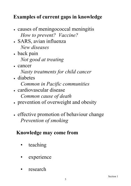
Examples of research questions that
- Page 300 and 301:
Example 1: What is the prevalence o
- Page 302 and 303:
Example 3: Is there an association
- Page 304 and 305:
Prospective Studies • groups are
- Page 306 and 307:
Confidence interval for relative ri
- Page 308 and 309:
Confidence interval for attributabl
- Page 310 and 311:
Case control studies • a group of
- Page 312 and 313:
a/ b The odds ratio, OR = c/ d = 32
- Page 314 and 315:
so a a c c ≈ and ≈ b a+ b d c+
- Page 316 and 317:
Chi Square Test for Contingency Tab
- Page 318 and 319:
We wish to know whether the data in
- Page 320 and 321:
Using this formula, expected number
- Page 322 and 323:
Example: For the drug responses, χ
- Page 324 and 325:
• the p-value gives the probabili
- Page 326 and 327:
Example 5 Is there an association b
- Page 328 and 329:
χ 2 2 (100−108.99) (107−111.01
- Page 330 and 331:
This page for reference only Income
- Page 332 and 333:
(a) OR = 1.90 with CI (1.23, 2.92)
- Page 334 and 335:
0 1 1.5 2 3 3.5 a x b x c d e x x x
- Page 336 and 337:
with υ = 1 degree of freedom. Sinc
- Page 338 and 339:
COMBINED ADMIT DECLINE Male 490 (44
- Page 340 and 341:
SOLUTIONS 29 1. (b) Risk (aspirin g
- Page 342 and 343:
SECTION 9 This section introduces t
- Page 344 and 345:
Regression methods are used to intr
- Page 346 and 347:
BAC X X X • • • • X X X X X
- Page 348 and 349:
FEV + + + + + + + + + + + + + + + +
- Page 350 and 351:
80 Y X 70 60 X X X 50 X X 40 X 100
- Page 352 and 353:
The method of least squares finds t
- Page 354 and 355:
N.B. 1. In this situation we have r
- Page 356 and 357:
important as they represent the err
- Page 358 and 359:
To illustrate, the example has x =
- Page 360 and 361:
That is, the total variation is par
- Page 362 and 363:
The F-distribution (Table in Append
- Page 364 and 365:
5. For the validity of the F-test,
- Page 366 and 367:
2. The divisor is (n - 2) rather th
- Page 368 and 369:
x i y i ( y − yˆ ) i i ( y − 1
- Page 370 and 371:
Stress (X) 55 94 64 73 96 86 Blood
- Page 372 and 373:
Confidence Interval for Prediction
- Page 374 and 375:
Y Prediction Interval X EXAMPLE: 20
- Page 376 and 377:
(c) (3 marks) What is the predicted
- Page 378 and 379:
(b) Estimated standard error = 3.47
- Page 380 and 381:
The denominator in formula for r is
- Page 382 and 383:
2 ( y i − y) ( x − x)( y − y)
- Page 384 and 385:
2. r = -1 is smallest value which i
- Page 386 and 387:
Some examples on correlation and as
- Page 388 and 389:
REVIEW EXERCISES 1. Physical fitnes
- Page 390 and 391:
SECTION 10 Multiple regression mode
- Page 392 and 393:
• The type of multiple regression
- Page 394 and 395:
The multiple linear regression mode
- Page 396 and 397:
Example For lung transplantation it
- Page 398 and 399:
It appears total lung capacity incr
- Page 400 and 401:
Step 3: Fit (in R-cmdr) Multiple Li
- Page 402 and 403:
The fitted equation is therefore ŷ
- Page 404 and 405:
It is 6.98 - 5.20 = 1.78 litres whe
- Page 406 and 407:
Are all three variables needed in t
- Page 408 and 409:
Test of the hypothesis H 0 : β 1 =
- Page 410 and 411:
95% confidence interval for coeffic
- Page 412 and 413:
Checking the fit of the model We do
- Page 414 and 415:
The points in the normal P-P plot l
- Page 416 and 417:
Analysis of Covariance This analysi
- Page 418 and 419:
At this stage the ages have been ig
- Page 420 and 421:
[C] Third, a regression analysis of
- Page 422 and 423:
The confidence interval here is the
- Page 424 and 425:
Notes: 1. 2 ˆβ (the coefficient o
- Page 426 and 427:
The logistic regression model is:
- Page 428 and 429:
(1) Investigating the relationship
- Page 430 and 431:
BUT what about the potential confou
- Page 432 and 433:
SECTION 11 Study design principles,
- Page 434 and 435:
Critical appraisal Critical apprais
- Page 436 and 437:
1. Introduction to critical apprais
- Page 438 and 439:
2. Design and appraisal of Descript
- Page 440 and 441:
Recall Suppose we want to estimate
- Page 442 and 443:
Selection bias • systematic error
- Page 444 and 445:
Example Life in New Zealand Survey,
- Page 446 and 447:
Internal validity Bias Selection bi
- Page 448 and 449:
Study design and critical appraisal
- Page 450 and 451:
Types of design: • experimental (
- Page 452 and 453:
Example Does smoking cause coronary
- Page 454 and 455:
Assessing internal validity: Bias S
- Page 456 and 457:
Evaluation and control of bias •
- Page 458 and 459:
Example of confounding: A study was
- Page 460 and 461:
Positive and Negative Confounding P
- Page 462 and 463:
Some comments on confounding: AGE a
- Page 464 and 465:
(3) Control of confounding during t
- Page 466 and 467:
Basic structure of a RCT • popula
- Page 468 and 469:
The way in which patients are alloc
- Page 470 and 471:
Randomised controlled trials : Exam
- Page 472 and 473:
Key results 849 randomised placebo
- Page 474 and 475:
Internal validity Chance • 95% co
- Page 476 and 477:
Intention-to-treat analysis “once
- Page 478 and 479:
Study design and critical appraisal
- Page 480 and 481:
Prospective cohort study (concurren
- Page 482 and 483:
Selection of participants • 5,766
- Page 484 and 485:
Bias Selection bias • because the
- Page 486 and 487:
Case-control studies Ref: “Case-C
- Page 488 and 489:
Selection of participants Study pop
- Page 490 and 491:
Key results Response rates: Cases:
- Page 492 and 493:
In this study: • the odds ratios
- Page 494 and 495:
Information bias Things done to min
- Page 496 and 497:
Generalisability Could we apply the
- Page 498 and 499:
Appendix One: The Basics This appen
- Page 500 and 501:
Example 3 If Z = X − μ calculate
- Page 502 and 503:
There are no hard and fast rules co
- Page 504 and 505:
Converting Fractions to Decimals Th
- Page 506 and 507:
X − μ Example 1: If Z = , calcul
- Page 508 and 509:
7. Sigma means Add Up The Greek let
- Page 510 and 511:
Section 2: Basic Statistical Concep
- Page 512 and 513:
5. Quartiles and Interquartile Rang
- Page 514 and 515:
9. If 1.96 X − 2.8 = , calculate
- Page 516 and 517:
• Probability of B given A: Pr( A
- Page 518 and 519:
Summary of Formulae 1. Normal Distr