SAMPLE OF A PROCEEDINGS PAPER:

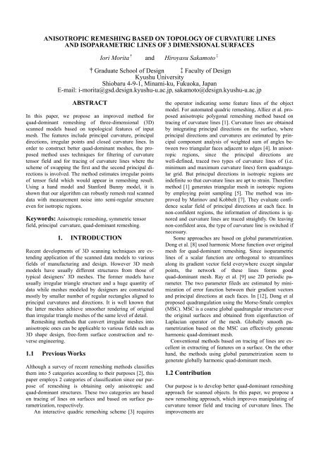
ANISOTROPIC REMESHING BASED ON TOPOLOGY OF CURVATURE LINES
AND ISOPARAMETRIC LINES OF 3 DIMENSIONAL SURFACES
Iori Morita † and Hiroyasu Sakamoto ‡
†Graduate School of Design ‡Faculty of Design
Kyushu University
Shiobaru 4-9-1, Minami-ku, Fukuoka, Japan
E-mail: i-morita@gsd.design.kyushu-u.ac.jp, sakamoto@design.kyushu-u.ac.jp
ABSTRACT
In this paper, we propose an improved method for
quad-dominant remeshing of three-dimensional (3D)
scanned models based on topological features of input
mesh. The features include principal curvature, principal
directions, irregular points and closed curvature lines. In
order to construct better quad-dominant meshes, the proposed
method uses techniques for filtering of curvature
tensor field and for tracing of curvature lines where the
scheme of swapping the first and the second principal directions
is involved. The method estimates irregular points
of tensor field which would appear in remeshing result.
Using a hand model and Stanford Bunny model, it is
shown that our algorithm can robustly remesh real scanned
data with measurement noise into semi-regular structure
even for isotropic regions.
Keywords: Anisotropic remeshing, symmetric tensor
field, principal curvature, quad-dominant remeshing.
1. INTRODUCTION
Recent developments of 3D scanning techniques are extending
application of the scanned data models to various
fields of manufacturing and design. However 3D mesh
models have usually different structures from those of
typical designers’ 3D meshes. The former models have
usually irregular triangle structure and a huge quantity of
data while meshes modeled by designers are constructed
mostly by smaller number of regular rectangles aligned to
principal curvatures and directions. It is well known that
the latter meshes achieve smoother rendering of original
than irregular triangle meshes of the same level of detail.
Remeshing methods that convert irregular meshes into
anisotropic ones can be applicable to various fields such as
3D shape design, free-form surface construction and reverse
engineering.
1.1 Previous Works
Although a survey of recent remeshing methods classifies
them into 5 categories according to their purposes [2], this
paper employs 2 categories of classification since our purpose
of remeshing is obtaining only anisotropic and
quad-dominant structures. These two categories are based
on tracing of lines on surfaces and based on surface parametrization,
respectively.
An interactive quadric remeshing scheme [3] requires
the operator indicating some feature lines of the object
model. For automated quadric remeshing, Alliez et al. proposed
anisotropic polygonal remeshing method based on
tracing of curvature lines [1]. Curvature lines are obtained
by integrating principal directions on the surface, where
principal directions and curvatures are estimated by principal
component analysis of weighted sum of angles between
two triangular faces adjacent to edges [4]. In anisotropic
regions, since the principal directions are
well-defined, traced two types of curvature lines of (i.e.
minimum and maximum curvature lines) form quadrangular
grid. But principal directions in isotropic regions are
indefinite so that curvature lines are apt to strain. Therefore
method [1] generates triangular mesh in isotropic regions
by employing point sampling [5]. The method was improved
by Marinov and Kobbelt [7]. They evaluate confidence
scalar field of principal directions at each face. In
non-confident regions, the information of directions is ignored
and curvature lines are traced straightly. On leaving
non-confident area, the type of curvature line is switched if
necessary.
Some approaches are based on global parametrization.
Dong et al. [8] used harmonic Morse function over original
mesh for quad-dominant remeshing. Since isoparametric
lines of a scalar function are orthogonal to streamlines
along its gradient vector field everywhere except singular
points, the network of these lines forms good
quad-dominant mesh. Ray et al. [9] use 2D periodic parameter.
The two parameter fileds are estimated by minimization
of error function between their gradient vectors
and principal directions at each faces. In [12], Dong et al
proposed quadrangulation using the Morse-Smale complex
(MSC). MSC is a coarse global quadrangular structure over
the original surfaces and obtained from eigenfunction of
Laplacian operator of the mesh. Globally smooth parametrization
based on the MSC can effectively generate
harmonic quad-dominant mesh.
Conventional methods based on tracing of lines are excellent
in extracting of features on a surface. On the other
hand, the methods using global parametrization seem to
generate globally harmonic quad-dominant mesh.
1.2 Contribution
Our purpose is to develop better quad-dominant remeshing
approach for scanned objects. In this paper, we propose a
new remeshing approach, which improves manipulating of
curvature tensor field and tracing of curvature lines. The
improvements are

(1) propagating principal directions from characteristic
curvature lines into isotropic regions,
(2) a detection method of irregular points,
(3) an extended tracing method of curvature lines with
swapping principal directions,
(4) searching and tracing methods of closed curvature
lines.
The propagating method aligns principal directions in
isotropic regions with directions of characteristic lines of
the shape. The detection method uses only anisotropic
components of the curvature tensor in order of robust detection
(section 2.2). The traced curvature lines from detected
irregular points are important topological characteristics
of the 3D shape.The extended tracing method exploits
swapping of the 1st and the 2nd principal directions
(section 3.1) in order to prevent crooking of lines and generate
better quad-dominant meshes. Since closed curvature
lines are important topological characteristics on models
such as generalized cylinders, the approach uses 2D parametrization
to search for closed lines (section 3.2).
By these improvements, the proposed remeshing approach
generates better quad-dominant remshes.
2. ANALYSIS OF GEOMETRIC PROPERTY
To trace curvature lines, we need to integrate the field of
principal directions. In this chapter, we describe how to
estimate principal curvature, direction and tensor fields and
filtering of these fields. An original input mesh of our algorithm
is an unstructured triangle mesh.
2.1 Estimation of Curvature Tensor
Let p be a vertex of original mesh with adjacent faces { f i |
i = 1,…, M} and n-ring neighboring vertices { q i | i =
1,…,N }. The face f i has barycentor f i and unit normal vector
n(f i ). We estimate normal vectors at p from PCA of following
matrix M.
= ∑
M 1
T
M ( p)
n(
fi)
n(
fi)
(1)
i 1 f p
=
i
−
where T means transpose. Among M(p)’s unit eigenvectors
e 1 , e 2 , e 3 , normal vector at p is estimated by the nearest
vector e 3 to the averaged normal vector n . The direction
of e 2 is the cross product of e 1 and e 3 .
n ( p)
= e , e = e × e
3 2 1 3
The neighboring vertices q i are transformed to x i .
T
T
x [ ] [ ]
i
= x
i
yi
zi
= e1 e2
e3
( qi
− p)
In order to estimate principal curvatures and directions,
the following quadric surface f is fitted to the points x i to
minimize the following error function E.
1
f ( x,
y)
= −
2
E =
N
2
2
( ax + 2bxy
+ cy + d )
∑( f ( xi
, yi
) − zi
)
i=
0
2
(2)
The 4 coefficients a, b, c, d are computed by linear equation.
The associated shape operator matrix of f can be decomposed
into rotation matrix and diagonal matrix of curvatures.
⎡a
⎢
⎣b
b⎤
⎡ cosθ
⎥ = ⎢
c⎦
⎣−
sinθ
sinθ
⎤⎡κ1
⎥⎢
cosθ
⎦⎣
0
0 ⎤⎡cosθ
⎥⎢
κ 2 ⎦⎣sinθ
−sinθ
⎤
⎥
cosθ
⎦
where κ 1 > κ 2 , θ is the signed angle between the 1st principal
direction and e 1 . In addition, we define 4 principal
directions including K 3 and K 4 .
K1(
p)
= R(
n(
p),
θ ) ⋅e1
K 2 ( p)
= K1(
p)
× n(
p)
K3(
p)
= −K1(
p),
K 4 ( p)
= −K
2 ( p)
where R(n, θ ) is rotation matrix about axis n and signed
angle θ . If the both of principal curvatures at p are equal,
the p is an umbilic point (isotropic region). If |κ 1 ||κ 2 |, Κ 2
and Κ 4 are directions of a ridge. We call these directions
feature directions.
The parameter field in a triangle face is obtained by linear
interpolation of the parameters at the 3 vertices. The
magnitude of anisotropy at p is shown by κ 1 (p) − κ 2 (p).
2.2 Filtering of Curvature Tensor
In this section, we smooth the fields of the principal curvatures
and directions using curvature tensors. The principal
curvatures and directions assigned on 3D surface are
shown by second order symmetric tensor field.
2.2.1 Smoothing
3D principal directions {Κ j j = 1,…,4 } at p and its
neighboring vertices should be embedded into tangent
plane at p. Using the 1st principal directions Κ 1 (p) and
Κ 2 (p) as basis vectors, the curvature tensor at p is
⎡κ
1(
p)
T(
p)
= ⎢
⎣ 0
0 ⎤
κ ( )
⎥
2
p ⎦
The tensor T(p) is smoothed by averaging over neighboring
vertices q i . In order to align coordinate axes of tensors
T(q i ) with that of T(p), we determine rotation matrix
E(α i,j ).
⎡cosαi,
j
− sinαi,
j ⎤
E ( αi,
j
) = ⎢
⎥
(6)
⎣sinαi,
j
cosαi,
j ⎦
where α i,j is signed angle between K 1 (p) and K j (q i ) which
gives minimum absolute angle |α i,j | among j = 1,2,3,4. The
curvature tensor at q i is computed as follows.
( ) 0
T
⎡κ
j qi
⎤
T( qi
) = E(
αi, j ) ⎢
E(
αi,
j )
0 κ j 1(
qi
)
⎥ (7)
⎣
+ ⎦
where the subscript j+1 is taken cyclical. The smoothed
tensor field is computed by weighted average of T.
∑i
∑
N
i=
1
(3)
(5)
T(
p)
+ w
=
iT(
q
1
i )
T ( p)
←
(8)
N
1+
w
i
where w i is 1 or a weight function such as Gaussian kernel.
The method can compute a smoother tensor field and
reduce the number of umbilic points. But we cannot obtain
trustworthy curvature tensors over wide isotropic region by
(4)

this smoothing process only, because the principal directions
at isotropic region are sensitive to noise of small
bumps and often show undesirable directions.
2.2.2 Propagation of Principal Directions
Our algorithm traces curvature lines along principal directions
for anisotropic remeshing. Therefore ambiguous principal
directions in isotropic regions often cause crooked
curvature lines and irregular points of resulting mesh. In
order to align the directions in isotropic region, the directions
of feature lines in anisotropic region are propagated
into neighboring isotropic regions.
Procedure. We set two constant c 1 and c 2 where c 1 > c 2 >
0. We pick up all vertices p where κ 1 (p)−κ 2 (p) > c 1 , then
we trace curvature lines from each vertex toward both of
forward and backward feature directions. Curvature lines
are traced until κ 1 (x)−κ 2 (x)

3.1 Swapping of Curvature Directions
In [1], curvature lines are traced based on integration of the
1st and the 2nd principal directions separately. The method
has problems that lines crook in regions such as waved
surface where the 1st and the 2nd directions are switching.
In order to reduce such crooking effects, we propose a
method for swapping directions of line tracing.
We use 4th-order Runge-Kutta mothod to trace a curvature
line on a triangle mesh. From a start point specified on
original mesh, we integrate vector field to trace a curvature
line. If a curvature line crosses the edge between face f i and
f j at p, we call the point p exit point of f i and entrance point
of f j . The present algorithm stores a series of the points p as
a curvature line.
Each vertex of mesh has four principal directions K j
(j=1,…,4). At each vertex of a triangle face f j , our method
selects one of the four principal directions which has the
closest direction to tangent vector d(p) at the entrance point.
The vector field for integration is evaluated by linear interpolation
of selected vectors at 3 vertices.
3.2 Closed Curvature Lines
Closed curvature lines are often regarded as important features.
For example, a rotational model has closed circles on
the surface. The closed curves on generalized cylinder can
be exploited in various applications such as seamless texture
mapping, detection of rotational axis and animation
based on the skeleton.
We detect closed curvature lines on surfaces as the first
clue of forming network of lines. If a curvature line
L + traced from a start points x 0 goes around the original
mesh and approaches to x 0 again, we similarly trace L −
from x 0 toward the counter directions of L + . If L − approaches
similarly, we detect a closed curvature line based
on the following parametrization procedure.
Two parameter fields U + (q) and U − (q) are assigned to the
neighbor regions of L + and L − , respectively.
⎡
+
⎤ ⎡
+
T
+ u ( q)
length(L
, x + ⎤
0,
xi
) Wi
Q
U ( q)
= ⎢ ⎥ =
+ ⎢
⎥ (16)
⎣v
( q)
⎦ ⎢⎣
( q − xi
) ⋅ b(
xi
) ⎥⎦
⎡
−
⎤ ⎡
−
T
− u ( q)
length(L
, x + ⎤
0,
xi
) Wi
Q
U ( q)
= ⎢ ⎥ =
− ⎢
⎥ (17)
⎣v
( q)
⎦ ⎢⎣
− ( q − xi
) ⋅ b(
xi
) ⎥⎦
We compute averaged 2D parameter field U(q).
⎡u(
q)
⎤
⎡
⎢ ⎥ = ⎢
⎣v(
q)
⎦ ⎢
⎣
+
−
( u ( q)
+ C − u ( q)
)/
2
( ) ( ) ⎥ ⎥ ⎤
+
−
+ v ( q)
− v ( q)
C − u ( q)
+ C − u ( q)
C
C ⎦
(18)
where C is averaged circumference of L + and L − . If q does
not belong to neighborhood of L − but L + , U(q) = U + (q), and
vice versa.
Isoparametric lines of parameter v(q) are closed lines on
the surface. We employ the isoparametric line v(q) = 0 as a
closed curvature line. We demonstrate an example of hand
model in Fig.2. Closed curvature lines are detected on the
wrist, thumb and fingers.
Fig. 2: Closed curvature lines.
3.3 Termination of Curvature Lines
Our method terminates line tracing on some conditions in
order to prevent the network from becoming too dense.
Tracing of a curvature line stops where the line satisfies
one of the following four conditions (1)-(4).
While tracing j-th curvature lines L j , short curvature lines
S i + and S i − are traced along both b(x i ) and −b(x i ) directions
from x i where x i is a sampling point on L j . If S i + is intersected
first by L k at the point y i , we call L k a neighbor line
of L j . The conditions for terminating of the tracing process
are,
(1) the line is close to a predicted irregularity,
(2) the line becomes longer than a constant,
(3) the number of neighbor line k is equal to j,
(4) the Euclid distance between y j and x j is smaller than
following c(κ,ε).
⎛ 2 ⎞
1
c ( κ,
ε ) = 2 ε ⎜ − ε ⎟ , 0 < ε <
(19)
⎝ | κ | ⎠
κ
Here, ε is a tolerance based on distance between a straight
line and an arc with radius |κ|, and κ is curvature corresponding
to the bi-normal directions of L i .
4. REMESHING USING NETWORK
In this section, we describe how to grow the network of
curvature lines. Curvature lines are increased by generating
new lines from seed points spaced on lines already added
to the network.
4.1 Detection of Closed Lines
In the first step, our algorithm searches the original mesh
for strong anisotropic points as candidates of start points of
closed lines and invests closed lines in the descending order
of strength of anisotoropy. If a start points is immediate
with existent closed line, it is excepted from candidates.
In the second step, our algorithm traces curvature lines
from the predicted irregular points. If neither closed lines
nor irregular points are detected, curvature line traced from
the strongest anisotropic vertex and adds the line to network.
4.2 Growth of Network
In the third step, our algorithm generates new lines from
lines of former steps. Seed points are sampled on each line

of current network according to Eq.(19). Assuming J as the
total number of lines, our algorithm follows the procedure
described below.
Procedure Firstly, seed points {x i } are put on the current
line L j . The interval between x i and x i+1 is determined by
c(κ,ε) and a ceiling. Secondly, new curvature lines are generated
from each x i. From all x i , two lines are traced respectively
along both b(x i ) and −b(x i ) directions until terminal
points described in 3.3. If the sum of lengths of them
is larger than a given constant, these lines are added to the
network as L J+1 , then J is increased by 1. If the sum is
smaller, these lines are deleted.
We repeat this procedure from j = 1 until j reach to J.
4.3 Elongation of Curvature Lines
The terminal points of curvature lines cause irregular
points (T-junction) in the resulting mesh. In order to reduce
the number of irregular points and broader adjustment of
the mesh, the curvature line L j is elongated until one of the
following conditions is satisfied.
(1) L j approaches to other terminal point of curvature line,
(2) L j is close to one of detected irregular points.
If the elongated part of a curvature line does not meet these
conditions in a given constant length, the part is deleted. In
Fig.3, the elongated parts of curvature lines are shown by
thicker lines. The circles denote detected irregular points.
5. EXPERIMANTAL RESULTS
One of resulting network is shown Fig.5(a). The original
data has 29,800 vertices. We set the tolerance ε and the
ceiling to 0.01 and 0.2, respectively. In this experiment,
number of vertices in remeshed data is 3,180. The back
part of the hand model containes waved surface. Such a
region cause crooked curvature lines by the conventional
method [1] as shown in Fig.5(b). This algorithm can
remesh such a region as regular as possible by swapping of
directions.
Figure 6 shows remeshing of Bunny model by proposed
algorithm, where Fig.6(a) is the original unstructured
mesh, and Figs. (b) and (c) are remeshed model rendered
by the flat shading and the smooth shading, respectively.
6. CONCLUSIONS
In this paper, we propose a quad-dominant remeshing algorithm
based on topology of curvature lines. This approach
can construct better quad-dominant meshes by filtering of
tensor fields and extended tracing of curvature lines. We
plan experimentation about various input meshes to evaluate
our methods. In addition, we consider introducing more
interactive application.
Fig. 3: Elongation of curvature lines
4.4 Post-processing
(a)
Although our algorithm makes quadrangle faces from the
network almost everywhere, terminal and irregular points
form polygonal faces, besides quadrangle such as upper
row of Fig.4 in the resulting mesh. In post-processing step,
these faces are subdivided for quad-dominant remeshing.
(b)
Fig. 4: Post-processing of terminal
and irregular points
Fig. 5: Network generated by proposed algorithm(a)
and conventional method(b)

Fig.6: Remeshing of Bunny model.
REFERENCE
[1] Alliez,P., Cohen-Steiner,D., Devillers.O, Levy,B.and
Desbrun,M., "Anisotropic Polygonal Remeshing,"
ACM Tras. Graphics, Proc. SIGGRAPH 2003, Vol. 22,
pp. 485-493, 2003.
[2] Alliez,P., Ucelli,G., Gotsman,C. and Attene,M., "Recent
Advances in Remeshing of Surfaces.", in Shape
Analysis and Structuring, ed. Floriani,L.D.and Spagnuolo,M.
pp.53-82, Springer, 2008
[3] Kanai.T, Suzuki.F, "An Interactive Remeshing method
for uniform meshes", Visual Computing/Graphics and
CAD, Joint Workshop ,pp.91-96, 2001 .
[4] Cohen-Steiner,D. and Morvan,J.,”Restricted Delaunay
triangulations and normal cycle.”, In Proc. ACM
Symposium on Computational Geometry, pp.312-321,
2003.
[5] Alliez,P., Colin de Verdiere,E.Devillers,O. and Isenburg,M.,
”Isotropic surface remeshing”,Procedings of
Shape Medeling International, pp.49-58, 2003.
[6] Surazhsky,V., Alliez,P. and Gotsman,C.,“Isotropic
remeshing of surfaces, a local parametrization approach”
In Proceedings of 12th International Meshing
Roundtable, pp.215-224, 2003
[7] Marinov,M. and Kobbelt,L., “Direct Anisotropic
Quad- Dominant Remeshing”, Proc. Computer
Graphics & Applications, pp.207-216, 2004.
[8] Dong,S. Kircher,S. and Garland,M., “Harmonic functions
for quadrilateral remeshing of arbitrary manifolds.”
Computer Aided Geometric Design, 2005.
[9] Ray,N., Li,W.C, Lévy,B., Sheffer,A. and Alliez,P., “Periodic
Global Parameterization”, ACM Trans. Graphics,
25, pp. 1460-1485, 2006.
[10] Petitjean,S. “A Survey of Meshed for Recovering
Quadrics in Triangle Meshes”, ACM Computing Survey,
2, pp.1-61, 2002
[11] Delmarcell,T. and Hesselink,L.,”The Topology of
Smmetric, Second-Order Tensor Fields.”,Proc. IEEE
Visualization Comf., pp.140-147, 1994
[12] Dong,S., Bremer,R,T., Gerland,M.,Pascucci,V. and
Hart,J,C., “Spectral Surface Quadrangulation”, ACM
Tras. Graphics, Proc. SIGGRAPH 2006, Vol. 25, pp.
1057-1066, 2006.