HIGH-FREQUENCY MODEL OF MONOTUBE SHOCK ABSORBERS

MODELOWANIE INŻYNIERSKIE ISSN 1896-771X
39, s. 81-88, Gliwice 2010
HIGH-FREQUENCY MODEL OF MONOTUBE SHOCK ABSORBERS
JANUSZ GOŁDASZ
BWI Group, Technical Center Kraków, ul. Podgórki Tynieckie 2, 30-399 Kraków, PL
e-mail: janusz.goldasz@bwigroup.com
Summary. It has been long recognized that the inertia and compressibility of the
fluid have an impact on the dynamic behaviour of semi-active monotube shock
absorbers utilizing so-called smart ER/MR fluids at high frequencies of the
system operation. Previous studies which dealt with analytical state-space & CFD
models of the magnetorheological shock absorber in a monotube configuration
indicated that any conventional analytical model is lightly damped and not
suitable for dynamic studies above 100-150 Hz. Therefore, in the present paper
the author illustrates an analytical model of a monotube shock absorber that is
suitable for high-frequency studies. In particular, the study presents a comparison
between the CFD results and the new model. Finally, the shock absorber
characteristics in the form of Bode plots of amplitude and frequency are presented
within a prescribed range of frequencies.
1. INTRODUCTION
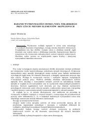
Investigation of the dynamic behavior of Magneto-Rheological (MR) & Electro-
Rheological shock absorbers [5,6,7] subjected to a small-stroke, medium- to high-frequency
excitation has revealed some interesting characteristics best described as a clockwise rotation
of the damping force vs. displacement characteristic curves (“ellipses”) with increasing
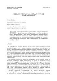
stroking frequency. The same phenomenon is responsible for the hysteretic behavior seen in
the force vs. piston velocity characteristic curves as shown in Figures 1 and 2. In Reference
[1] the author makes the hypothesis that the likely contributors is the fluid inertia and the
compressibility, and describes a fairly detailed force-driven model of the damper incl. the
compressibility of fluid chambers, laminar losses through the piston annular flow path, and
the inertia of the fluid element occupying the annulus. Both piston and rod assembly (P&R)
inertia were taken into account. The numerical calculation carried out in [1] identified two
vibration modes. The primary one relates to the fluid element dynamic, whereas the second
(higher) resonant frequency is due to the combined inertia of the P&R and the fluid element.
As a result, in Reference [2] an observation was made that the P&R inertia has little or no
effect under normal working conditions, and can be eliminated leading to a simplified reduced
order stroke-driven model that describes adequately the MR damper dynamics for frequencies
up to the first natural frequency of the damper.
The purpose of the present study is to extend the earlier analytical model for the simplest
model configuration presented in Reference [2], and further analyzed in Reference [3] against
Computational Fluid Dynamics (CFD) data. When compared against the CFD results, it
became clear the analytical model of [2] would be lightly damped at the higher frequency

82 J. GOŁDASZ
regime, and a mechanism for accounting for the viscosity (and the inertia) of the fluid
throughout the damper should be investigated and added to the analytical models in order to
improve its fidelity at frequencies near the resonance. As such, in the present paper a
hydraulic network type model of a shock absorber is designed and tested in order to confirm
the CFD study conclusions. Therefore, in Section 2.1 the author outlines the hydraulic
network approach and the dynamic model of the shock absorber, and Section 2.2 contains
details of the CFD experiment performed by the author in order to test the network model.
Sections 2.3 and 2.4 contain damper configuration specific data and damper test setup
information, respectively. Finally, the results are presented in Section 2.5 and the conclusions
drawn in Section 3.
1000
800
600
10 Hz
15 Hz
20 Hz
25 Hz
400
Force, [N]
200
0
-200
-400
-600
-800
-1000
-1 -0.8 -0.6 -0.4 -0.2 0 0.2 0.4 0.6 0.8 1
Speed, [m/s]
Figure 1. Off-state (zero current) force-velocity phase plane
1000
800
600
10 Hz
15 Hz
20 Hz
25 Hz
400
Force, [N]
200
0
-200
-400
-600
-800
-1000
-6 -3 0 3 6
Stroke, [mm]
Figure 2. Off state force-displacement phase plane

HIGH-FREQUENCY MODEL OF MONOTUBE SHOCK ABSORBERS 83
2. MODELING AND SIMULATIONS
2.1. Shock absorber model
Consider the monotube damper configuration shown in Figure 3 and the simplified
configuration in Figure 4. The cylinder tube houses the floating piston (gas cup) which
separates the fluid from the pressurized gas. The main piston separates the upper and lower
fluid chambers and includes an annular passage to permit the fluid to flow from one chamber
to the other. In the present study the annulus is approximated by flat-plate geometry of length
(area) L g (A g ). The shock absorber fluid is characterized by the three parameters: the density ρ,
the bulk modulus β, and the viscosity μ; the magnetic field is absent, and the fluid behavior is
Newtonian. Therefore, the fluid flow through the annulus produces viscous damping forces.
Figure 3. Monotube damper configuration [1]
Figure 4. Reduced (velocity-driven) damper configuration
and its lumped parameter model [2]
In order to account for the viscous losses across the whole shock absorber volume, the
fluid volumes on either side of the main piston were modeled as a hydraulic network of
inertia, compliance and viscous resistance elements. Figure 5 shows the lumped parameter
approximation of mass-spring portion of the (compliant) fluid volume. The inertia factor of a
single lump of length L i (and the volume V 0,i ) is then equal to ρL i /A i , whereas the compliance
of the lump is β/V 0,i . The annulus cross-sectional area is A i . .Then, the corresponding
equations of motion for the lump i at mid-stroke conditions are as follows
ìdQi
ï =
Ai
P
ï
dt ρLi
ïdPin
β
i
í =
ï dt V 0, i
ïdPout
β
i
ï
=
î dt V0,
i
128µ
Li
Ri
4
πd
i
( - - )
in
P
( Q -Q
)
in
( Q -Q
)
i
out
i
out
RiQ
i
= (2)
(1)

84 J. GOŁDASZ
where P in , P out are the pressures in and out of the lump, and Q in , Q out are the volume flow rates
associated with the pressures, respectively. R i accounts for the hydraulic resistance of the
lump, and d i refers to the lump hydraulic diameter. Assuming laminar flow losses, the term
can be given by Equation 2. For example, the equations of motion of a model consisting of
three lumps (N=3) can be described in the following manner
ì dP1
β
ï
= (-Q
)
1
dt
ï
V 0,1
ïdQ1
=
A1
ï
P1
P2
dt ρL1
ï
ï
dP2
β
=
1 Ap
ï dt V 0,2
ïdQ2
Ag
í = P2
P3
ï
dt ρLg
ïdP3
β
ï
=
2 Ap
dt V 0,3
ï
ïdQ3
=
A3
P3
P4
ï dt ρL3
ï
ï
dP4
β
= ( Q3)
ïî
dt V0,4
( - - )
R1Q
( Q + v -Q
)
( - - Q )
R
( Q - v -Q
)
( - - Q )
where v is the input velocity of the piston. In the above model shown in Figure 6 the flow
rates Q 2 , Q 3 and the pressures P 2 and P 3 , respectively, drive the motion of the fluid element
contained in the annular gap of the main piston. The area of the piston is A p . The remaining
variables account for the behavior of the corresponding fluid lumps. Note the above equations
correspond to the simplified shock absorber configuration with no gas chamber in Figure 4.
R
3
p
1
2
3
3
2
(3)
Figure 5. Hydraulic network lump
Figure 6. Hydraulic network model; N=3
As a result, the damping force across the piston can be obtained from
= ( )
(4)
F
A
P
P
d p 2 - 3
The equation set can be easily cast into the state-space form, thus yielding
T
where X = [ P1
P2
P3
P4
Q1
Q2
Q3]
. Therefore,
dX
= AX + Bv
(5)
dt

HIGH-FREQUENCY MODEL OF MONOTUBE SHOCK ABSORBERS 85
A =
0
0
0
0
A1
ρL
0
0
1
0
0
0
0
A1
-
ρL
A2
ρL
0
2
1
0
0
0
0
0
A2
-
ρL
A3
ρL
3
2
0
0
0
0
0
0
A3
-
ρL
3
β
-
V
β
V
0,2
0
0
0,1
A1
- R1
ρL
0
0
1
β
-
V
β
V
- R
0
2
0,2
0,3
0
0
0
A2
ρL
2
β
-
V
β
V
0
0
0,3
0,4
0
0
A3
- R3
ρL
3
(6)
B =
0
0
0
0
0
0
0
0
0
0
0
0
0
0
0
0
0
0
0
0
0
0
0
0
0
0
0
0
0
2
β
A
V 0,2
A2
- β
V
0
from which the (linear) network transfer function between the output force and the input
velocity can be easily deduced in an analytical fashion.
2.2. CFD model
The FLUENT unsteady 2D-axisymmetric model configuration shown in Figure 7
corresponds to the simple shock absorber model explored in [2] and shown in Figure 4; the
reader should refer to the paper for further information. Shortly, the piston rod is neglected,
and the piston motion is prescribed as a sinusoidal velocity profile to reflect the actual testing
conditions of real dampers. In the analysis dynamic layering algorithm in FLUENT was used
to adjust the model mesh according to the prescribed motion profile. Finally, the damping
force was obtained by integrating pressure distributions on either side of the piston.
0
0
0
0,3
0
0
0
0
0
0
0
0
0
0
0
0
0
0
(7)
Figure 7. CFD monotube damper model
(only the annulus with adjacent regions is shown) [3]

86 J. GOŁDASZ
2.3. Actuator Geometry and Material Properties
Table 1 reveals the key actuator dimensions and material properties used in the analytical
model setup as well as the CFD analysis.
2.4. Test setup
Table 1. Actuator geometry and material properties
Parameter
Value
Fluid dynamic viscosity
30 cP
Bulk modulus
220 MPa
Fluid density
2.5 g/cc
Area factor 1662 mm 2
Annulus size
0.7 mm
Annulus length
30 mm
Annulus area 80 mm 2
Chamber length
100 mm
No. of lumps, N {1,3,5}
The CFD model is exercised in such a manner to copy the testing of real shock absorbers
on a hydraulic stroker, i.e., the cylinder tube is fixed while the piston is stroked with a
sinusoidal constant-velocity profile at discrete frequencies (and with ever-decreasing
displacement). The stroking frequencies range from 3 to 390 Hz, as the stroke is varied from
the peak-to-peak value of 16 mm down to 0.12 mm at the final frequency of 390 Hz. As a
consequence, the peak velocity of the driving piston is held constant at 0.15 m/s at all
frequencies.
Clearly, the hydraulic network model is exercised in a manner similar to that of the CFD
experiment to enable a direct comparison of the model performance against the CFD data.
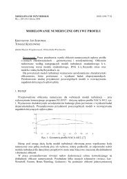
2.5. Results
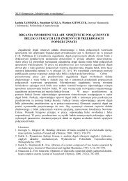
To analyze the influence of the number of lumps in the hydraulic network model numerical
tests involving the model with N={1, 3, 5} lumps were performed within the prescribed range
of input frequencies, respectively. The results are presented in Figures 9-10 as plots of the
amplitude and phase angle against frequency. At first, the model was configured with the
laminar model in the flow path for both piston and cylinder sections. In general, the linear
approach is not satisfactory even for the relatively low speed regime considered in the study.
While the linear model approaches the natural frequency of the CFD model as the number of
lumps increases, the damping force amplitude at that frequency is still overestimated by a
factor of 3 (for a model with 5 lumps). Therefore, the author decided to enhance the each
lump with a hydraulic resistance term that is proportional to flow rate squared ( Qi2 ) to account
for entry/exit losses in the annulus, for example. The magnitude of these components was
estimated from CFD steady-state tests. Adding the quadratic damping term improved the
model. As seen in Figures 8, 9 and 10, it can be noted that the modified network model is
approaching the natural frequency of the shock absorber and the amplitude as well as phase.
The model, however, still overestimates the amplitude of the damping force at resonance.

HIGH-FREQUENCY MODEL OF MONOTUBE SHOCK ABSORBERS 87
4000
3500
CFD
MODEL
MODEL: 268 Hz
3000
]
[
N
,
e
c
r
o
F
2500
2000
1500
CFD: 220 Hz
1000
500
0
10 0 10 1 10 2 10 3
Frequency, [Hz]
Figure 8. CFD vs. state-space model [3]
2000
N=1
N=3
N=5
CFD Results
MOD. MODEL (N=1): 268 Hz
1500
]
[
N
,
e
c
o
F
1000
CFD: 220 Hz
500
0
10 0 10 1 10 2 10 3
Frequency, [Hz]
Figure 9. Force vs. frequency; modified hydraulic network model
3. SUMMARY AND CONCLUSIONS
The purpose of the paper was to illustrate the analytical model of a monotube shock
absorber that is suitable for engineering purposes. That model can be used in higher frequency
vehicle suspension simulations instead of more complex CFD or phenomenological models.
In order to account for damping in the cylinder sections of the damper as well as fluid
compressibility and inertia, the (simplified) device was modeled as a hydraulic network of
lumped mass, compliance and viscous resistance elements. For comparison, the previous
analytical models [1,2] assumed viscous losses only in the annulus of the piston and inviscid
fluid elsewhere. When compared to the CFD experiment, the models were lightly damped. It
seems the hydraulic network is better at capturing the natural frequency of the model.
However, the model still overestimates the damping force at that frequency which indicates
some work on the damping (viscous loss) component of the network model is still required.

88 J. GOŁDASZ
100
50
]
g
e
[
d
,
e
s
a
h
P
0
-50
N=1
N=3
N=5
-100
150 200 250 300 350 400
Frequency, [Hz]
Figure 10. Phase shift vs. frequency; modified hydraulic network model
REFERENCES
1. Alexandridis A. A., Gołdasz, J.: High-frequency Dynamics of Magneto-Rheological
Dampers. In: Proceedings of the Ninth International Conference on New Actuators
(“ACTUATOR 2004”), Bremen, Germany, 14-16 June, 2004.
2. Alexandridis A. A, Gołdasz J.: Simplified model of the dynamics of magneto-rheological
dampers. “Mechanics” 2005, Vol. 24(2), p. 47-53.
3. Gołdasz, J., Alexandridis A. A.: Frequency-dependent behavior of MR dampers: CFD
Study. In: Proceedings of the Active Noise and Vibration Control Methods Conference
(“MARDiH 2007”), Krasiczyn, Poland, 11-14 June, 2007.
4. Peel D. J., Stanway R., Bullough W. A.: Dynamic modeling of ER vibration damper for
vehicle suspension applications. „Smart Materials and Structures“ 1996, Vol. 5, p. 591-
606.
5. Hopkins P. N.: Magnetorheological fluid damper. US Patent 6311810, 2001.
6. Petek, N.: Adjustable dampers using electrorheological fluids. US Patent 5259487, 1993.
7. Nguyen Q.-H., Choi S.: A new approach for dynamic modeling of an electrorheological
damper using a lumped parameter method, Nguyen, Quoc-Hung; Choi, Seung-Bok,
“Smart Materials and Structures” 2009, Vol. 18(11), p. 115 – 120.