II II II II II I - Waste Isolation Pilot Plant - U.S. Department of Energy

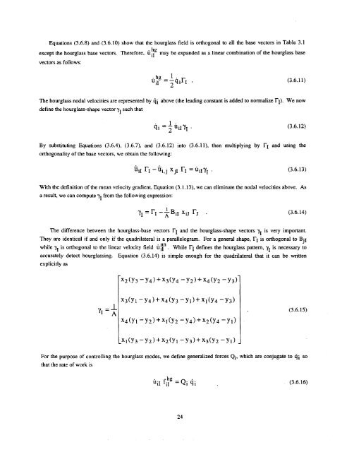
Equations (3.6.8) and (3.6.10) show that the hourglass field is orthogonal to all the base vectors in Table 3.1
hg
except the hourglass base vectors. Therefore, u il may be expanded as a linear combination of the hourglass base
vectors as follows:
(3.6.11)
The hourglass nodal velocities are represented by ~i above (the leading constant is added to normalize rI). We now
define the hourglass-shape
vector yl such that
qi ‘~uiI~l . (3.6.12)
13y substituting Equations (3.6.4), (3.6.7), and (3.6.12) into (3.6.11), then multiplying by rI and using the
orthogonality of the base vectors, we obtain the following:
iiiI rI ‘iii,j XJI rI = uiI~l . (3.6.13)
With the definition of the mean velocity gradient, Equation (3.1.13), we can eliminate the nodal velocities above. As
a result, we can compute ‘yIfrom the following expression:
YI=rI–~BiI xiJ rJ . (3.6.14)
The difference between the hourglass-base vectors rI and the hourglass-shape vectors ‘yI is very important.
They are identical if and only if the quadrilateral is a parallelogram. For a general shape, rI is orthogonal to BjI
while yl is orthogonal to the linear velocity field u y. while rI defines the hourglass pattern, II is necessary to
accurately detect hourglassing. Equation (3.6. 14) is simple enough for the quadrilateral that it can be written
explicitly
as
‘2(Y3 ‘y4)+x3b’4 ‘Y2)+X4(Y2 ‘Y3)
x3(yl–y4)+ x4(y3–yl) +xl(y4–y3)
~1=*
(3.6.15)
x4(yl–y2) +xl(y2–y4) +x2(y4–yl)
LX,(YS‘Y2)+XZ(Y, ‘Y3)+X3(Y2 ‘YI)
For the purpose of controlling the hourglass modes, we define generalized forces Qi, which are conjugate to ~i so
that the rate of work is
‘g= Qiqi .
U iI fi~ (3.6.16)
24