II II II II II I - Waste Isolation Pilot Plant - U.S. Department of Energy

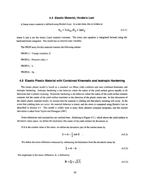
4.4 Elastic Material, Hooke’s Law
A linear elastic material is defined using Hooke’s Law. In a rate form, this is written as
blj =L(dkk)~ij + z~dij (4.4.1)
where L and w are the elastic Lam6 material constants. The stress rate equation is integrated forward using the
backward Euler integrator. The model has no internal state variables.
The PROP array for this material contains the following entries:
PROP(1) - Young’s modulus, E
PROP(2) - Poisson’s ratio, v
PROP(3) - %
PROP(4) - 2y .
4.5 Elastic Plastic Material with Combined Kinematic and Isotropic Hardening
The elastic plastic model is based on a standard von Mises yield condition and uses combined kinematic and
isotropic hardening. Isotropic hardening is the behavior where the radius of the yield surface grows equally in all
directions due to plastic straining. Kinematic hardening is the behavior where the radius of the yield surface remains
constant, but the center of the yield surface translates in the direction of the plastic strain rate. In this discussion of
the elastic plastic material model, .we assume that the material is yielding and that plastic straining will occur. In the
event that yielding does not occur, the material behavior is elastic and the stress is computed using Hooke’s Law as
described in Section 4.4. This model is widely used in many finite element computer programs, and the current
derivation is taken from Taylor and Flanagan ( 1987).
Some definitions and assumptions are outlined here. Referring to Figure 4.5.1, which shows the yield surface in
deviatoric stress space, we define the backstress (the center of the yield surface) by the tensor, et.
If 6 is the current value of the stress, we define the deviatoric part of the cument stress by
S=+(T5 .
(4.5.1)
We define the stress difference measured by subtracting the backstress from the deviatoric stress by
(4.5.2)
The magnitude of the stress difference, R, is defined by
R’lq=lm (4.5.3)
36