Polynomiography: A New Intersection between ... - Nikkemedia.fi
Polynomiography: A New Intersection between ... - Nikkemedia.fi
Polynomiography: A New Intersection between ... - Nikkemedia.fi

Create successful ePaper yourself
Turn your PDF publications into a flip-book with our unique Google optimized e-Paper software.
<strong>Polynomiography</strong>: A <strong>New</strong> <strong>Intersection</strong> <strong>between</strong> Mathematics and Art 1<br />
Bahman Kalantari<br />
Department of Computer Science, Rutgers University<br />
Hill Center, <strong>New</strong> Brunswick, NJ, 08903<br />
<strong>Polynomiography</strong> is de<strong>fi</strong>ned to be “the art and science of visualization in approximation of<br />
the zeros of complex polynomials, via fractal and non-fractal images created using the mathematical<br />
convergence properties of iteration functions.” An individual image is called a “polynomiograph.”<br />
The word polynomiography is a combination of the word “polynomial” and the<br />
suf<strong>fi</strong>x “-graphy.” It is meant to convey the idea that it represents a certain graph of polynomials,<br />
but not in the usual sense of graphing, say a parabola for a quadratic polynomial.<br />
Polynomiographs are obtained using algorithms requiring the manipulation of thousands of<br />
pixels on a computer monitor. Depending upon the degree of the underlying polynomial, it is<br />
possible to obtain beautiful images on a laptop computer in less time than a TV commercial.<br />
Polynomials form a fundamental class of mathematical objects with diverse applications;<br />
they arise in devising algorithms for such mundane task as multiplying two numbers, much<br />
faster than the ordinary way we have all learned to do this task (FFT). According to the<br />
Fundamental Theorem of Algebra, a polynomial of degree n, with real or complex coef<strong>fi</strong>cients,<br />
has n zeros (roots) which may or may not be distinct. The task of approximation of the zeros of<br />
polynomials is a problem that was known to Sumerians (third millennium B.C.). This problem<br />
has been one of the most influential problem in the development of several important areas in<br />
mathematics. <strong>Polynomiography</strong> offers a new approach to solve and view this ancient problem,<br />
while making use of new algorithms and today’s computer technology. <strong>Polynomiography</strong> is<br />
based on the use of one or an in<strong>fi</strong>nite number of iteration functions designed for the purpose<br />
of approximation of the roots of polynomials. An iteration function is a mapping of the plane<br />
into itself, i.e. given any point in the plane, it is a rule that provides another point in the plane.<br />
<strong>New</strong>ton’s iteration function is the best known : N(z) =z − p(z)/p ′ (z). An iteration function<br />
can be viewed as a machine that approximates a zero of a polynomial by an iterative process<br />
that takes an input and from it creates an output which in turn becomes a new input to the<br />
same machine.<br />
The word “fractal,” which partially appears in the de<strong>fi</strong>nition of polynomiography, was coined<br />
by the world-renowned research scientist Benoit Mandelbrot. It refers to sets or geometric<br />
objects that are self-similar and independent of scale. This means there is detail on all levels of<br />
magni<strong>fi</strong>cation. No matter how many times one zooms in, one can still discover new details. It<br />
turns out that some fractal images can be obtained via simple iterative schemes leading to sets<br />
known as Julia sets and the famous Mandelbrot set. The simplicity of these iterative schemes,<br />
which may or may not have any signi<strong>fi</strong>cant purpose in mind, has resulted in the creation of<br />
numerous web sites in which amateurs and experts exhibit their fractal images. Many fractal<br />
images pertain to the famous Mandelbrot set.<br />
<strong>Polynomiography</strong>, on the other hand, has a well-de<strong>fi</strong>ned and focused purpose in mind.<br />
It makes use of one or an in<strong>fi</strong>nite number of iteration functions for polynomial root-<strong>fi</strong>nding.<br />
1 c○2000 Bahman Kalantari. All Rights Reserved<br />
1
A polynomiograph may or may not result in a fractal image. This is one of the reasons it<br />
was necessary to give a new name to this process. A second reason is because its purpose<br />
is the visualization of a polynomial, via approximation of its roots and the way in which<br />
the approximation is carried out. Even when a polynomiograph is a fractal image it does not<br />
diminish its uniqueness. The assertion that an image is a fractal image is no more profound than<br />
asserting that an image is a picture, or a painting. In particular, that assertion does not capture<br />
any artistic values of the image. Indeed, even in terms of fractal images polynomiography reveals<br />
a vast number of possibilities and degrees of freedom and results in a wider variety of images<br />
than typical fractal images.<br />
<strong>Polynomiography</strong> could become a new art form. Working with polynomiography software<br />
is comparable to working with a camera or a musical instrument. Through practice, one can<br />
learn to produce the most exquisite and complex patterns. These designs, at their best, are<br />
analogous to the most sophisticated human designs. The intricate patterning of Islamic art,<br />
the composition of Oriental carpets, or the elegant design of French fabrics come to mind<br />
as very similar to the symmetrical, repetitive, and orderly graphic images produced through<br />
polynomiography. But polynomiographic designs can also be irregular, asymmetric, and nonrecurring,<br />
suggesting parallels with the work of artists associated with Abstract Expressionism<br />
and Minimalism. <strong>Polynomiography</strong> could be used in classrooms for the teaching of art or<br />
mathematics, from children to college-level students, as well as in both professional and nonprofessional<br />
situations. Its creative possibilities could enhance the professional art curriculum.<br />
The “polynomiographer” can create an in<strong>fi</strong>nite variety of designs. This is made possible<br />
by employing an in<strong>fi</strong>nite variety of iteration functions (which are analogous to the lenses of<br />
a camera) to the in<strong>fi</strong>nite class of complex polynomials (which are analogous to photographic<br />
models). The polynomiographer then may go through the same kind of decision making as<br />
the photographer: changing scale, isolating parts of the image, enlarging or reducing, adjusting<br />
values and colors until the polynomiograph is resolved into a visually satisfying entity. Like<br />
a photographer, a polynomiographer can learn to create images that are esthetically beautiful<br />
and individual, with or without the knowledge of mathematics or art. Like an artist and a<br />
painter, a polynomiographer can be creative in coloration and composition of images. Like a<br />
camera, or a painting brush, a polynomiography software can be made simple enough that even<br />
a child could learn to operate it.<br />
Despite the signi<strong>fi</strong>cant role of the root-<strong>fi</strong>nding problem in the development of fundamental<br />
areas, today it is not considered to be a central problem in pure or computational mathematics.<br />
According to a 1997 article in SIAM Review by Victor Pan [28], a leading authority on the<br />
computational complexity aspects of the root-<strong>fi</strong>nding problem, in practice often one needs to<br />
compute roots of polynomials of very moderate degree (10 or 20), except possibly in computer<br />
algebra which is applied to algebraic optimization and algebraic geometry. In view of the above<br />
and since there are already ef<strong>fi</strong>cient subroutines for computing roots of moderate size polynomials,<br />
it would not be surprising that many may view the polynomial root-<strong>fi</strong>nding problem as one<br />
that has basically reached a dead-end. However, I believe that polynomiography will change<br />
all of this, not only from the mathematical or scienti<strong>fi</strong>c point of view, but from the educational<br />
and artistic point of view.<br />
Quoting the great American mathematician Smale [34], “There is a sense in which an important<br />
result in mathematics is never <strong>fi</strong>nished.” The Fundamental Theorem of Algebra is one<br />
of those results. To me polynomiography is a good evidence in support of Smale’s statement.<br />
With the availability of a good polynomiography software, the user (who may be a high school<br />
student, an artist, or a scientist) is quite likely to wish to experiment with much larger degree<br />
polynomials than degree 10 or 20. In particular, this is true because in polynomiography there<br />
2
is a “reverse root-<strong>fi</strong>nding problem”: given a polynomial whose roots form a known set of points,<br />
<strong>fi</strong>nd an iteration method whose corresponding polynomiograph would take a desired pattern.<br />
In principle, using this reverse problem, I can conceive of the blue print to some of the most<br />
elegant patterns, for instance carpets designs, yet to be woven. Their complexity and beauty<br />
could very well increase by increasing the degree size. Thus, it is conceivable that the implementation<br />
of such designs would demand working with much more computer power than that<br />
offered by a laptop computer, perhaps a supercomputer, or a network of computers.<br />
Mathematical Foundation of <strong>Polynomiography</strong><br />
Consider the polynomial<br />
p(z) =a n z n + a n−1 z n−1 + ···+ a 1 z + a 0 ,<br />
where n ≥ 2, and the coef<strong>fi</strong>cients a 0 ,...,a n are complex numbers. The problem of approximating<br />
the roots of p(z) is a fundamental and classic problem. A large bibliography can be found in<br />
[25]. For an article on some history, applications, and new algorithms, see Pan [28]. Some of the<br />
root-<strong>fi</strong>nding methods <strong>fi</strong>rst obtain a high-precision approximation to a root, then approximate<br />
other roots after deflation, see e.g., Jenkins and Traub [10]. Many such root-<strong>fi</strong>nding methods<br />
make use of iteration functions, e.g. <strong>New</strong>ton’s or Laguerre’s. A method that guarantees convergence<br />
to all the roots was given by Weyl [38]. This method is a two-dimensional analogue<br />
of the bisection method. Modi<strong>fi</strong>cations of this method has been used to obtain an initial approximation<br />
to a root, followed by the use of <strong>New</strong>ton’s method with a guaranteed estimate on<br />
the complexity of approximation, see e.g. Renegar [31], Pan [27]. Another root-<strong>fi</strong>nding method<br />
is based on recursive factorization of the given polynomial, see e.g. Kirrin [23]. Many deep<br />
theoretical complexity results on polynomial root-<strong>fi</strong>nding and/or the use of <strong>New</strong>ton’s method,<br />
are known, see e.g. Smale [34, 35], Shub and Smale [32, 33], Friedman [6]. Many topics on<br />
polynomials can be found in [1], and [2].<br />
One of the conceptually easiest algorithms for the approximation of all the roots of polynomials<br />
is described in Kalantari [20], making use of a fundamental family of iteration functions<br />
called the “Basic Family.” The algorithm reveals a magical pointwise convergence of the family<br />
to roots (see Theorem 2). The Basic Family is represented as {B m (z)} ∞ m=2 . The algebraic<br />
development and some optimal properties of the Basic Family are studied in [12], [13]. The<br />
<strong>fi</strong>rst member of the sequence, B 2 (z), is <strong>New</strong>ton’s iteration function, and B 3 (z) is Halley’s iteration<br />
function [9]. For the rich history of these two iteration functions alone see Ypma [39] and<br />
Traub [36]. In particular, Halley’s method inspired the celebrated Taylor’s Theorem (see [39]).<br />
Many results on the properties of the members of this family including their close ties with a<br />
determinantal generalization of Taylor’s Theorem can be found in [12]-[22].<br />
The members of the Basic Family have an interesting closed formula. Let p(z) beapolynomial<br />
of degree n ≥ 2 with complex coef<strong>fi</strong>cients. Set D 0 (z) ≡ 1, and for each natural number<br />
m ≥ 1, de<strong>fi</strong>ne<br />
⎛<br />
⎞<br />
p ′ p<br />
(z)<br />
′′ (z) p<br />
2!<br />
...<br />
(m−1) (z) p (m) (z)<br />
(m−1)! (m)!<br />
p(z) p ′ .<br />
(z) .. . .. p (m−1) (z)<br />
(m−1)!<br />
D m (z) =det<br />
. 0 p(z) .. . .. .<br />
,<br />
⎜<br />
⎝<br />
.<br />
. . .. . ⎟<br />
.. p ′′ (z) ⎠<br />
2!<br />
0 0 ... p(z) p ′ (z)<br />
3
⎛<br />
p ′′ (z)<br />
2!<br />
p ′ (z)<br />
̂D m,i (z) =det<br />
p(z)<br />
⎜<br />
⎝ .<br />
p ′′′ (z)<br />
3!<br />
...<br />
p ′′ (z)<br />
2!<br />
p ′ (z)<br />
.<br />
p (m) (z)<br />
(m)!<br />
. .. p (m−1) (z)<br />
(m−1)!<br />
. ..<br />
.<br />
.<br />
. .. p ′′ (z)<br />
2!<br />
0 0 ... p ′ (z)<br />
p (i) (z)<br />
i!<br />
p (i−1) (z)<br />
(i−1)!<br />
.<br />
.<br />
p (i−m+2) (z)<br />
(i−m+2)!<br />
p (i−m+1) (z)<br />
(i−m+1)!<br />
where i = m +1,...,n+ m − 1, and det(·) represents determinant.<br />
For each m ≥ 2, de<strong>fi</strong>ne<br />
B m (z) ≡ z − p(z)<br />
D m−2(z)<br />
D m−1 (z) .<br />
Note that D m (z) corresponds to the determinant of a Toeplitz matrix de<strong>fi</strong>ned with respect<br />
to the normalized derivatives of p(z). A square matrix is called Toeplitz if its elements are<br />
identical along each diagonal.<br />
Some of the fundamental properties of the members of the Basic Family are described in<br />
the following theorem. Its second part, in particular is a very special case of a nontrivial<br />
determinantal generalization of Taylor’s theorem given in [15].<br />
Let C be the <strong>fi</strong>eld of complex numbers. For a complex number c = a + ib, wherei = √ −1,<br />
its modulus is |c| = √ a 2 + b 2 .<br />
Theorem 1. Kalantari [16, 20]) The following conditions hold:<br />
1. For all m ≥ 1wehave,<br />
D m (z) =<br />
n∑<br />
i=1<br />
(−1) i−1 pi−1 (z)p (i) (z)<br />
i!<br />
2. Let θ be a simple root of p(z). Then,<br />
⎞<br />
,<br />
⎟<br />
⎠<br />
D m−i (z), D j =0, j < 0.<br />
m+n−2<br />
∑<br />
B m (z) =θ + (−1) ̂D m m−1,i (z)<br />
D m−1 (z) (z − θ)i .<br />
i=m<br />
3. There exists r>0 such that given any a 0 ∈ N r (θ) ={z : |z − θ| ≤r}, the <strong>fi</strong>xed-point<br />
iteration a k+1 = B m (a k ) is well-de<strong>fi</strong>ned, and it converges to θ having order m. Speci<strong>fi</strong>cally,<br />
(θ − a k+1 )<br />
lim<br />
̂D m−1,m (θ)<br />
k→∞ (θ − a k ) m =(−1)m−1 p ′ (θ) m−1 .<br />
4. Let θ be a simple root of p(z). There exists a neighborhood of θ, N ∗ (θ), such that for<br />
each a within this neighborhood p ′ (a) ≠0,|a − θ| < 1, and<br />
|p ′ (a)|−<br />
n∑<br />
i=0,i≠1<br />
|p(a)| i−1<br />
2<br />
|p (i) (a)|<br />
i!<br />
≥ 1 2 |p′ (a)|.<br />
For any a ∈ N ∗ (θ), if we set<br />
[ n∑ ( |p (i) )<br />
(a)| 2 ] 1/2<br />
h(a) =<br />
,<br />
i!<br />
i=0<br />
4
then we have<br />
∣ |B m (a) − θ| ≤<br />
2h(a) ∣∣∣ m( )<br />
∣ p ′ (a) (a − θ) 1<br />
.<br />
1 −|a − θ|<br />
5. In particular, if θ is a simple root of p(z), there exists r ∗ ∈ (0, 1) such that given any<br />
a ∈ N r ∗(θ), we have<br />
θ = lim<br />
m→∞ B m(a).<br />
6. D m (a) and hence B m (a) can be computed in O(n log n log m) operations.<br />
To describe a fundamental global convergence property of the sequence let<br />
R p = {θ 1 ,...,θ t }<br />
be the set of distinct roots of p(z). The elements of R p partition the Euclidean plane into<br />
Voronoi regions and their boundaries. The Voronoi region of a root θ is a convex polygon<br />
de<strong>fi</strong>ned by the locus of points which are closer to this root than to any other root. More<br />
precisely, the Voronoi region of a root θ is<br />
V (θ) ={z ∈ C : |z − θ| < |z − θ ′ |, ∀ θ ′ ∈ R p , θ ′ ≠ θ}.<br />
Let S p be the locus of points that are equidistant from two distinct roots, i.e.<br />
S p = {z ∈ C : |z − θ| = |z − θ ′ |, where θ, θ ′ ∈ R p , θ ≠ θ ′ }.<br />
This is a set of measure zero consisting of the union of a <strong>fi</strong>nite number of lines.<br />
De<strong>fi</strong>nition 1. Given a ∈ C the Basic Sequence at a is de<strong>fi</strong>ned as<br />
Theorem 2. ([20])<br />
satisfying<br />
B m (a) =a − p(a) D m−2(a)<br />
, m =2, 3,....<br />
D m−1 (a)<br />
Given p(z), for any input a ∉ S p , the Basic Sequence is well-de<strong>fi</strong>ned<br />
lim<br />
m→∞ B m(a) =θ,<br />
for some θ ∈ R p . Under some regularity assumptions, e.g. simplicity of all the roots of p(z),<br />
for all a ∈ V (θ), lim m→∞ B m (a) =θ.<br />
Remark. The determinantal generalization of Taylor’s theorem given in part 2 of Theorem<br />
1 gives a mechanism for estimating the error |B m (a) − θ|. The Basic Sequence can be even<br />
de<strong>fi</strong>ned for functions that are not polynomial. In Kalantari [19] the pointwise evaluation of the<br />
Basic Family (the Basic Sequence in the terminology of De<strong>fi</strong>nition 1) is used to give new formulas<br />
for the approximation of π and e. In Kalantari [20] it is also shown how the relationship<br />
<strong>between</strong> the Basic Sequence and the Basic Family gives new results for general homogeneous<br />
linear recurrence relations that are de<strong>fi</strong>ned via a single nonzero initial condition.<br />
Basins of Attraction and Voronoi Regions of Polynomial Roots<br />
Consider a polynomial p(z) and a <strong>fi</strong>xed natural number m ≥ 2. The basins of attraction<br />
of a root of p(z) with respect to the iteration function B m (z) are regions in the complex plane<br />
such that given an initial point a 0 within them, the corresponding sequence a k+1 = B m (a k ),<br />
k = 0, 1,..., will converge to that root. It turns out that the boundary of the basins of<br />
5
attractions of any of the polynomial roots is the same set. This boundary is known as the<br />
Julia set and its complement it known as the Fatou set. The fractal nature of Julia sets and<br />
the images of the basins of attraction of <strong>New</strong>ton’s method are now quite familiar for some<br />
special polynomials. For example fractal image of p(z) =z 3 − 1 was apparently <strong>fi</strong>rst studied<br />
by the American mathematician John Hubbard while teaching calculus in France (see Gleick<br />
[8]). That image and similar images that are now quite familiar also appear in [26], as well as<br />
[37] (see also its references). Mandelbrot’s work (see The Fractal Geometry of Nature [24]) in<br />
particular popularized the Julia theory [11] on the iteration of rational complex functions, as<br />
well as the work of Fatou [5], and led to the famous set that bears Mandelbrot’s name. Peitgen<br />
et al. [30] undertake a further analysis of fractals. Mathematical analysis of complex iterations<br />
may be found in Peitgen and Richter [29], Devaney [3], and Falconer [4].<br />
While the fractal nature of the Julia sets corresponding to the individual members of the<br />
Basic Family follows from the Julia theory on rational iteration functions, that theory does not<br />
predict the total behavior of speci<strong>fi</strong>c iteration functions on the complex plane. For instance the<br />
Julia theory does not even predict the shapes of basins of attraction of the polynomial p(z) =<br />
z n − 1 for various members of the Basic Family. In contrast, there are important consequences<br />
of the results stated in Theorems 1 and 2 which apply to arbitrary polynomials. In particular,<br />
Theorem 2 implies the following: Except possibly for the locus of points equidistant to two<br />
distinct roots, given any input a, the Basic Sequence {B m (a) =a − p(a)D m−2 (a)/D m−1 (a)}<br />
converges to a root of p(z). Under some regularity assumption (e.g. simplicity of the roots),<br />
for almost all inputs within the Voronoi polygon of a root, the corresponding Basic Sequence<br />
converges to that root. The Basic Sequence corresponds to the pointwise evaluation of the<br />
Basic Family. Theorem 2 gives rise to a new set of non-fractal polynomiographs with enormous<br />
beauty.<br />
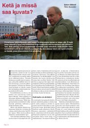
Figure 1 and Figure 2 present several fractal images that con<strong>fi</strong>rm the theoretical convergence<br />
results: as m increases, the basins of attraction of the roots, as computed with respect to the<br />
iteration function B m (z), rapidly converge to the Voronoi regions of the roots. Thus the regions<br />
with chaotic behavior rapidly shrink to the boundaries of the Voronoi regions.<br />
Figure 1 considers a polynomial with a random set of roots, depicted as dots. The <strong>fi</strong>gure<br />
shows the evolution of the basins of attraction of the roots to the Voronoi regions as m takes the<br />
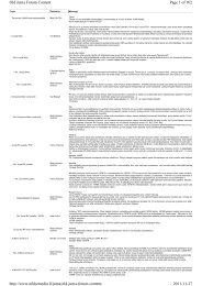
values 2, 4, 10, and 50. Figure 2 shows the basins of attraction for the polynomials p(z) =z 4 −1,<br />
corresponding to different values of m. The roots of p(z) =z 4 − 1 are the roots of unity and<br />
hence the Voronoi regions are completely symmetric. In these <strong>fi</strong>gures in the case of m = 2, i.e.<br />
<strong>New</strong>ton’s method, the basins of attraction are chaotic. However, these regions rapidly improve<br />
by increasing m.<br />
Figure 1: Evolution of basins of attraction to Voronoi regions via B m (z): random points,<br />
m =2, 4, 10, 50 (left to right).<br />
<strong>Polynomiography</strong> and Visual Arts<br />
I will <strong>fi</strong>rst describe some general techniques for the creation of polynomiographic images<br />
6
Figure 2: Evolution of basins of attraction to Voronoi regions via B m (z): p(z) = z 4 − 1,<br />
m =2, 3, 4, 50 (left to right).<br />
and exhibit sample images obtained via a prototype software for polynomiography, as well as<br />
provide an explanation of how some of these images were created. Subsequently, I will consider<br />
other applications of polynomiography.<br />
General Techniques for Creating Artwork<br />
In order to describe some general techniques for producing polynomiographic images I will<br />
<strong>fi</strong>rst describe the capabilities of prototype polynomiography software we have developed. The<br />
software allows the user to create an image by inputing a polynomial through several means,<br />
e.g. by inputing its coef<strong>fi</strong>cients, or the location of its zeros. In one approach the user simply<br />
inputs a parameter, m, as any natural number greater than one. The assignment of a value<br />
for m corresponds to the selection of B m (z) as the underlying iteration function. This together<br />
with the selection of a user-de<strong>fi</strong>ned rectangular region and user-speci<strong>fi</strong>ed number of pixels,<br />
tolerance, as well as a variety of color mapping schemes enables the user to create an in<strong>fi</strong>nite<br />
number of basic polynomiographs. These polynomiographs turn out to be fractal images and<br />
can subsequently be easily re-colored or zoomed in any number of times. A non-fractal and<br />
completely different set of images could result from the visualization of the root-<strong>fi</strong>nding process<br />
through the collective use of the Basic Family, i.e. the pointwise convergence property described<br />
in Theorem 2. These images are enormously rich. In either type of image creation technique<br />
the user has a great deal of choices, e.g. the ability to re-color any selected regions using a<br />
variety of coloration schemes based on convergence properties.<br />
Viewing polynomiography as an art form, one can list at least four general image creation<br />
techniques.<br />
(1) Like a photographer who shoots different pictures of a model and uses a variety of lenses,<br />
a polynomiographer can produce different images of the same polynomial and make use of a<br />
variety of iteration functions and zooming approaches until a desirable image is discovered.<br />
(2) In this more creative approach an initial polynomiograph, possibly very ordinary, is<br />
turned into a beautiful image, based on the user’s choice of coloration, individual creativity,<br />
and imagination. This is analogous to carving a statue out of stone.<br />
(3) The user employs the mathematical properties of the iteration functions, or the underlying<br />
polynomial, or both (this is truly a marriage of art and mathematics).<br />
(4) Images can be created as a collage of two or more polynomiographs produced through<br />
any one of the previous three methods.<br />
Many other image creation techniques are possible, either through artistic compositional<br />
means, or through computer assisted design programs.<br />
An Exhibition<br />
7
This section presents an exhibition of some polynomiographic images that I have created<br />
through the above four techniques. The reader may notice the diversity of these images. In<br />
particular, they contrast with literally hundreds of fractal images exhibited at web sites. It<br />
should be noted that the images displayed are not necessarily symmetric. These are given as<br />
Figure 3 - Figure 13. It should be mentioned that none of the images in the paper is displayed<br />
at its optimal size. Indeed the optimal size for the display of some of the images is poster size.<br />
This is because at that size we begin to see and appreciate the real complexity and detail of<br />
the images.<br />
In the near future an interactive version of a polynomiography software will become available<br />
at www.polynomiography.com, where the visitor will be able to input his/her own polynomial<br />
and obtain various polynomiographs.<br />
Figure 3: “Cathedral”, “Eiffel Tower”, “Party on Brooklyn Bridge”<br />
Figure 4: “Waltz”<br />
With the exception of some of the images in the “Evolution of Stars and Stripes”, and in<br />
8
Figure 5: “Mathematics of a Heart”, “Mona Lisa in 2001”, “Butterfly”<br />
Figure 6: All Untitled<br />
“Ms. Poly” all other images have resulted from a single input polynomial. In “Ms. Poly”<br />
all regions that depict different features come from a single polynomial, except for her lips,<br />
themselves a polynomiograph, which came from a different polynomial and were collaged.<br />
The Making of “Mona Lisa in 2001”<br />
A polynomial of degree 10 was used to produce the left polynomiograph in Figure 12. Then<br />
as a result of zooming in on one of the signi<strong>fi</strong>cant parts of that image, the right image in Figure<br />
12 was obtained. A coloration of various layers resulted in the <strong>fi</strong>nal image.<br />
The Making of “Mathematics of a Heart”<br />
One of the features of the software is to allow the user to enter a polynomial by placing the<br />
location of the roots on the working canvas of the computer monitor. The software then builds<br />
the polynomial from the roots. Subsequently, any one of the techniques can be applied. The<br />
image “Mathematics of a Heart” was produced by simply drawing a heart shape and then by<br />
applying one of the techniques, together with personal coloration.<br />
9
Figure 7: “Life and Death” (two views of the same polynomial)<br />
Figure 8: “Acrobats”, “Happy Birthday Hal!!!”<br />
The Making of “Evolution of Stars and Stripes”<br />
The inspiration to create a polynomiographic image of the U.S. flag came from Jasper Johns<br />
paintings of the flag. The <strong>fi</strong>rst image was conceived by making use of the convergence properties<br />
of the Basic Family and the fact that the basins of attraction converge to the Voronoi<br />
regions of the roots. The underlying polynomial for the <strong>fi</strong>rst image is a polynomial of degree<br />
5 whose roots consist of <strong>fi</strong>ve points on a vertical line. The second and third images are variations<br />
of the <strong>fi</strong>rst one. The star image was obtained from a single polynomial and is collaged<br />
(after reduction of size) onto the third image. The <strong>fi</strong>nal image comes from the coloration of a<br />
polynomiograph of a single polynomial (zoomed in at an appropriate area) together with the<br />
collage of white stars coming from a different polynomiograph than that of the evolving star.<br />
It is hoped that the <strong>fi</strong>ve images give the impression that the flag is evolving: the appearance of<br />
the stripes and the emergence of the color white (<strong>fi</strong>rst images); the close up of the <strong>fi</strong>rst image,<br />
while the evolution is in progress, which reveals the emergence of the color blue (second image);<br />
the creation of stars and the continuous growth and reshaping of white and blue regions (third<br />
image); a close-up of one of the forming stars which appear as if it is in rotation (fourth <strong>fi</strong>gure);<br />
and <strong>fi</strong>nally the orderly formations of various components of the flag and the settling of the<br />
stars. The conceptualization and creation of the <strong>fi</strong>ve images took more than the summer of 2000.<br />
10
Figure 9: “Evolution of Stars and Stripes”<br />
Figure 10: “Summer Variations”<br />
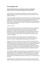
Symmetric Designs from <strong>Polynomiography</strong><br />
Symmetric designs can be obtained by considering polynomials whose roots have symmetric<br />
patterns. One can obtain interesting images by simply considering polynomials whose roots<br />
are the roots of unity or more generally n-th root of a real number r. By the multiplication<br />
of these polynomials, as well as the rotation of the roots one can obtain some very interesting<br />
basic designs that can subsequently be painted into beautiful designs. The images in Figure 13<br />
and Figure 16 are such examples.<br />
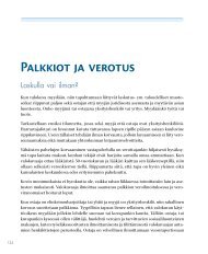
Polynomiographs of Numbers<br />
One interesting application of polynomiography is in the encryption of numbers, e.g. ID<br />
numbers or credit card numbers into a two dimensional image that resembles a <strong>fi</strong>ngerprint.<br />
Different numbers will exhibit different <strong>fi</strong>ngerprints. One way to visualize numbers as polynomiographs<br />
is to represent them as polynomials. For instance a hypothetical social security<br />
number a 8 a 7 ···a 0 can be identi<strong>fi</strong>ed with the polynomial P (z) =a 8 z 8 + ···+ a 1 z + a 0 . Now<br />
we can apply any of the techniques discussed earlier. A particularly interesting visualization<br />
results when the software makes use of the Basic Family collectively (see Theorem 2). Figures<br />
11
Figure 11: “Ms. Poly” and “L3”<br />
Figure 12: Polynomiographs leading to “Mona Lisa in 2001”<br />
14 gives several examples.<br />
The reader may notice that all of the images are distinct except possibly the two lower<br />
rightmost images. But that is because they are consecutive numbers. Upon closer look, Figure<br />
15, their differences can be noticed immediately. Now given such a polynomiograph for<br />
a number it should be possible to build scanners that can convert the image back into the<br />
original number. The conversion requires the recognition of the roots and the recovery of the<br />
corresponding polynomial coef<strong>fi</strong>cients.<br />
Public Use of <strong>Polynomiography</strong> in Arts and Design<br />
Through various software programs, polynomiography could grow into a new art form for<br />
both professional and non-professional art-making, and in the teaching of both art and mathematics.<br />
The recent proliferation of craft supply stores in the United States reveals the deep<br />
seated urge in the general population to create. Having polynomiography software available on<br />
home computers could release that creative power even more; people could invent their own<br />
knitting and needlepoint patterns, design their own carpets, and create simply for the sake of<br />
creating. The polynomiographic pattern in Figure 16 was motivated by a design from a Persian<br />
12
Figure 13: A polynomiograph of 10z 48 − 11z 24 +1<br />
carpet and made use of pointwise convergence described in Theorem 2. It is possible to obtain<br />
much more sophisticated patterns than this.<br />
At a more advanced level, polynomiography can be used to teach the fundamentals of design<br />
and color theory. While information science software has transformed the advanced graphic design<br />
curriculum through Photo Shop, Quark, and similar programs, the visual arts curriculum<br />
makes little use of information science at the fundamentals level. <strong>Polynomiography</strong> provides<br />
the opportunity to teach decision-making in composition, spatial construction, and color at a<br />
much more complex level than the present system which relies on the traditional methods of<br />
drawing and collage. Through using polynomiography software, students have in<strong>fi</strong>nite design<br />
possibilities before them. In making their selections, they can experiment with symmetry and<br />
asymmetry, repetition, unity, balance, spatial illusion, lines, and planes. By using color, they<br />
can gain understanding of complementary color, value relationships, and balance while learning<br />
to manipulate hue, tint, and intensity.<br />
<strong>Polynomiography</strong> and Education<br />
<strong>Polynomiography</strong> has enormous potential applications in education. A polynomiography<br />
13
Figure 14: A polynomiograph of six different nine digit numbers<br />
Figure 15: A polynomiograph of the numbers 672,123,450 and 672,123,451<br />
software could be used in the mathematics classroom as a device for understanding polynomials<br />
as well as the visualization of theorems pertaining to polynomials. As an example of one<br />
application of polynomiography, high school students studying algebra and geometry could be<br />
introduced to mathematics through creating designs from polynomials. They would learn to<br />
use algorithms on a sophisticated level and to understand the mathematics of polynomials in<br />
their relationship to pattern and design in ways that cannot be approached abstractly. For<br />
instance, Figure 14 can be viewed as a visualization of the Fundamental Theorem of Algebra,<br />
as applied to the polynomials corresponding to these numbers. It is possible to compile many<br />
theorems about polynomials and their properties, or those of iteration functions that can be<br />
visualizable through polynomiography. At a higher educational level, e.g. calculus or numerical<br />
analysis courses, polynomiography allows students to tackle important conceptual issues such<br />
as the notion of convergence and limits, as well as the idea of iteration functions, and gives the<br />
student the ability to understand and appreciate more modern discoveries such as fractals.<br />
There are also numerous algorithmic issues that are motivated by polynomiography, such as<br />
the development of even newer root-<strong>fi</strong>nding algorithms. <strong>Polynomiography</strong> is not only a means<br />
for obtaining fast algorithms for polynomial root-<strong>fi</strong>nding but also allows the users to determine<br />
how two particular members of the Basic Family compare. Which is better, <strong>New</strong>ton’s method<br />
or Halley’s method Most numerical analysis books do not bother with such questions. But<br />
indeed these are fundamental questions from a pedagogical and practical point of view. One<br />
may make use of fractal images to study the computational advantages of members of the Basic<br />
Family over <strong>New</strong>ton’s method, as well as the advantages in using the Basic Sequence in computing<br />
a single root, or all the roots of a given polynomial.<br />
14
Figure 16: A polynomiograph of a degree 36 polynomial<br />
Extensions of <strong>Polynomiography</strong> and Iteration Techniques<br />
In this paper, polynomiography has been introduced in terms of the properties of a fundamental<br />
family of iteration functions, namely the Basic Family. However, more generally<br />
polynomiography can be de<strong>fi</strong>ned with respect to any iteration function for polynomial root<strong>fi</strong>nding.<br />
While experimentation with polynomiographs of other iteration functions is likely to<br />
be interesting, many unique mathematical and computational properties of the Basic Family<br />
members makes them much more interesting than any other individual iteration function, and as<br />
a family more fundamental than any other family of iteration functions. There are still many<br />
mathematical properties of the family that need to be studied. Moreover, polynomiography<br />
could even be enhanced with multipoint versions of the Basic Family.<br />
A nontrivial determinantal generalization of Taylor’s formula proved in Kalantari [15], whose<br />
precise description is avoided here, plays a dual role in the approximation of a given function<br />
or its inverse (hence its roots). On the one hand, the determinantal Taylor formula unfolds<br />
each ordinary Taylor polynomial into an in<strong>fi</strong>nite spectrum of rational approximations to the<br />
given function. On the other hand, these formulas give an in<strong>fi</strong>nite spectrum of rational inverse<br />
approximations, as well as single and multipoint iteration functions that include the Basic<br />
Family. Given m ≥ 2, for each k ≤ m, weobtainak-point iteration function, de<strong>fi</strong>ned as the<br />
ratio of two determinants that depend on the <strong>fi</strong>rst m − k derivatives. These matrices are upper<br />
Hessenberg and for k = 1 also reduce to Toeplitz matrices. The corresponding iteration function<br />
is denoted by B m (k) . Their formula will not be given here. Their order of convergence, proved<br />
in Kalantari [14], ranges from m to the limiting ratio of the generalized Fibonacci numbers of<br />
order m.<br />
The following diagram represents the ascending order of convergence of B m (k) ,andthecorresponding<br />
orders for a partial table of iteration functions:<br />
B (1)<br />
2 ← B (2)<br />
2<br />
↓ ↓ ↘<br />
B (1)<br />
3<br />
← B (2)<br />
3<br />
← B (3)<br />
3<br />
↓ ↓ ↓ ↘<br />
B (1)<br />
4 ← B (2)<br />
4 ← B (3)<br />
4 ← B (4)<br />
4<br />
↓ ↓ ↓ ↓ ↘<br />
B (1)<br />
5 ← B (2)<br />
5 ← B (3)<br />
5 ← B (4)<br />
5 ← B (5)<br />
5<br />
↓ ↓ ↓ ↓ ... ↘<br />
2 ← 1.618<br />
↓ ↓ ↘<br />
3 ← 2.414 ← 1.839<br />
↓ ↓ ↓ ↘<br />
4 ← 3.302 ← 2.546 ← 1.927<br />
↓ ↓ ↓ ↓ ↘<br />
5 ← 4.236 ← 3.383 ← 2.592 ← 1.965<br />
↓ ↓ ↓ ↓ ... ↘<br />
15
The Basic Family is only the <strong>fi</strong>rst column of the above diagram. The practicality of the<br />
multipoints was considered in [22] which gave a computational study of the <strong>fi</strong>rst nine root<strong>fi</strong>nding<br />
methods. These include the <strong>New</strong>ton, secant, and Halley methods. Our computational<br />
results with polynomials of degree up to 30 revealed that for small degree polynomials B m<br />
(k−1) is<br />
more ef<strong>fi</strong>cient than B m (k) , but as the degree increases, B m<br />
(k) becomes more ef<strong>fi</strong>cient than B m (k−1) .<br />
The most ef<strong>fi</strong>cient of the nine methods is the derivative-free method B (4)<br />
4 , having a theoretical<br />
order of convergence equal to 1.927. <strong>New</strong>ton’s method which is often viewed as the method of<br />
choice is in fact the least ef<strong>fi</strong>cient method. More computational results and a bigger subset of<br />
the above in<strong>fi</strong>nite table could reveal further practicality of the multipoint iteration family.<br />
The properties of the Basic Family and the Basic Sequence give rise to new algorithmic<br />
strategies. When the given input a is close enough to a simple root of the underlying polynomial,<br />
for any m ≥ 2, the Basic Sequence can be turned into an iterative method of order m by<br />
replacing the given input a with B m (a), and repeating. There are many computational implications<br />
of these results. As an example, one possible algorithm for polynomial root-<strong>fi</strong>nding is<br />
the following: for a given input a continue producing B m (a) until the difference <strong>between</strong> B m (a)<br />
and B m+1 (a) is small. Then for a desirable m replace a with B m (a) and repeat in order to<br />
obtain higher and higher accuracy. It is also possible to switch back and forth <strong>between</strong> the two<br />
schemes.<br />
An algorithm suggested by the global convergence properties of the Basic Sequence in order<br />
to compute all the roots of a given polynomial is as follows: <strong>fi</strong>rst we obtain a rectangle that<br />
contains all the roots. Then, by selecting a sparse number of points we generate the corresponding<br />
Basic Sequence and thereby obtain a good approximation to a subset of the roots.<br />
Then after deflation the same approach can be applied to <strong>fi</strong>nd additional roots. This method<br />
could provide an excellent alternative to the method of Weyl [38] (see also Pan [28] for Weyl’s<br />
method). Experimentation with this method is intended and will be reported in the future.<br />
In addition to the above multipoint versions of the Basic Family, it is also possible to de<strong>fi</strong>ne<br />
an in<strong>fi</strong>nite “Truncated Basic Family,” as well as a “parameterized Basic Family.” Doing<br />
polynomiography with these will be the subject of future work. It would also be interesting to<br />
consider polynomiography with other families of iteration functions, e.g. the Euler-Schroeder<br />
family (see [13], [15]).<br />
Concluding Remarks and the Future of <strong>Polynomiography</strong><br />
In this paper I have described some general techniques for creating polynomiographic images.<br />
However, even with polynomiography software at one’s disposal, from the user’s point of view<br />
it is essential to have available a very detailed and systematic manual and/or a book. The<br />
creation of such publications is one of my future goals. Indeed different users will bene<strong>fi</strong>t from<br />
different such publications.<br />
It is believed that through various software programs polynomiography could not only grow<br />
into a new art form for both professional and non-professional art-making, but also into a tool<br />
with enormous applications in the teaching of art and mathematics. One polynomiography<br />
software can be used to teach both art and mathematics more effectively; and another can be<br />
used for the visualization of polynomial properties by advanced researchers. For instance, I can<br />
foresee that some mathematicians will become interested in studying the polynomiography of<br />
many important families of polynomials. <strong>Polynomiography</strong> can be used not only to teach about<br />
polynomials and polynomial root-<strong>fi</strong>nding, but also about the underlying notions, e.g. complex<br />
16
numbers and operations on them. Effective means of communications of artistic or educational<br />
aspects of polynomiography can best be achieved by collaboration with artists, mathematicians,<br />
and educators. This is another of my future plans.<br />
<strong>Polynomiography</strong> also provides a potentially powerful tool for architecture, furniture, and<br />
other kinds of design. Some two-dimensional polynomiographs can give rise to three-dimensional<br />
objects. These and other three-dimensional applications of polynomiography are yet another<br />
one of my future goals.<br />
Finally, I remark that some convergence properties of the Basic Family are extendable to<br />
more general analytic functions than polynomials. Thus, analogous to the case of polynomials,<br />
it is possible to visualize roots of these more general analytic functions. However, the ef<strong>fi</strong>ciency<br />
of the corresponding visualizations could dramatically decrease. For instance, applying the<br />
basic family to a rational function (quotient of two polynomials) is inef<strong>fi</strong>cient as we make use<br />
of higher order members of the Basic Family. From the visual point of view, the world of<br />
polynomials is already in<strong>fi</strong>nitely rich. Moreover, polynomials form an important class, which<br />
makes them very appealing for conveying many concepts. One of my present goals is to design a<br />
new course on the subject of polynomiography with the aim of bringing together students from<br />
art and science. While the title of this paper introduces polynomiography as an intersection<br />
<strong>between</strong> mathematics and art, I do believe that it enhances both areas.<br />
References<br />
[1] D.BiniandV.Y.Pan,Polynomials and Matrix Computations, Vol. 1: Fundamental Algorithms,<br />
Birkhäuser, Boston, Cambridge, MA, 1994.<br />
[2] P. Borwein and T. Erdélyi, Polynomials and Polynomial Inequalities, Vol. 161, Springer-Verlag,<br />
<strong>New</strong> York, 1995.<br />
[3] R. L. Devaney, Introduction to Chaotic Dynamic Systems, Benjamin Cummings, 1986.<br />
[4] K.J.Falconer,Fractal Geometry: Mathematical Foundations and Applications, John Wiley & Sons,<br />
1990.<br />
[5] P. Fatou, Sur les équations fonctionelles, Bull. Soc. Math. France, 47 (1919), 161-271.<br />
[6] J. Friedman, On the convergence of <strong>New</strong>ton’s method, J. of Complexity, 5 (1989), 12-33.<br />
[7] J. Gerlach, Accelerated convergence in <strong>New</strong>ton’s method, SIAM Review, 36 (1994), 272-276.<br />
[8] J. Gleick, Chaos: Making a <strong>New</strong> Science, Penguin Books, 1988.<br />
[9] E. Halley, A new, exact, and easy method of <strong>fi</strong>nding roots of any equations generally, and that<br />
without any previous reduction, Philos. Trans. Roy. Soc. London, 18 (1694), 136-145.<br />
[10] M.A. Jenkins and J.F. Traub, A three-stage variable-shift iteration for polynomial zeros and its<br />
relation to generalized Rayleigh iteration, Numer. Math., 14 (1970), 252-263.<br />
[11] G. Julia, Sur les équations fonctionelles, J. Math. Pure Appl., 4 (1918), 47–245.<br />
[12] B. Kalantari, and I. Kalantari, High order iterative methods for approximating square roots, BIT<br />
36 (1996), 395-399.<br />
[13] B. Kalantari, I. Kalantari, and R. Zaare-Nahandi, A basic family of iteration functions for polynomial<br />
root <strong>fi</strong>nding and its characterizations, J. of Comp. and Appl. Math., 80 (1997), 209-226.<br />
[14] B. Kalantari, On the order of convergence of a determinantal family of root-<strong>fi</strong>nding methods, BIT<br />
39 (1999), 96-109.<br />
17
[15] B. Kalantari, Generalization of Taylor’s theorem and <strong>New</strong>ton’s method via a new family of determinantal<br />
interpolation formulas and its applications, J. of Comp. and Appl. Math., 126 (2000),<br />
287-318.<br />
[16] B. Kalantari, Approximation of polynomial root using a single input and the corresponding derivative<br />
values, Technical Report DCS-TR 369, Department of Computer Science, Rutgers University,<br />
<strong>New</strong> Brunswick, <strong>New</strong> Jersey, 1998.<br />
[17] B. Kalantari, Halley’s method is the <strong>fi</strong>rst member of an in<strong>fi</strong>nite family of cubic order root-<strong>fi</strong>nding<br />
methods, Technical Report DCS-TR 370, Department of Computer Science, Rutgers University,<br />
<strong>New</strong> Brunswick, <strong>New</strong> Jersey, 1998.<br />
[18] B. Kalantari and J. Gerlach, <strong>New</strong>ton’s method and generation of a determinantal family of iteration<br />
functions, J. of Comp. and Appl. Math., 116 (2000), 195-200.<br />
[19] B. Kalantari, <strong>New</strong> formulas for approximation of π and other transcendental numbers, Numerical<br />
Algorithms 24 (2000), 59-81.<br />
[20] B. Kalantari, On homogeneous linear recurrence relations and Approximation of Zeros of Complex<br />
Polynomials, Technical Report DCS-TR 412, Department of Computer Science, Rutgers University,<br />
<strong>New</strong> Brunswick, <strong>New</strong> Jersey, 2000, To appear in DIMACS Proceedings on, Unusual Applications<br />
in Number Theory.<br />
[21] B. Kalantari, An in<strong>fi</strong>nite family of iteration functions of order m for every m, Department of<br />
Computer Science, Rutgers University, <strong>New</strong> Brunswick, <strong>New</strong> Jersey, forthcoming.<br />
[22] B. Kalantari and S. Park, A computational comparison of the <strong>fi</strong>rst nine members of a determinantal<br />
family of root-<strong>fi</strong>nding methods, J. of Comp. and Appl. Math., 130 (2001) 197-204.<br />
[23] P. Kirrinnis, Partial fraction decomposition in C(z) and simultaneous <strong>New</strong>ton iteration for factorization<br />
in C[z], J. of Complexity, 14 (1998), 378-444.<br />
[24] B. B. Mandelbrot, The Fractal Geometry of Nature, <strong>New</strong> York, W.F. Freeman, 1983.<br />
[25] J. M. McNamee, A bibliography on root of polynomials, J. of Comp. and Appl. Math., 47 (1993),<br />
391-394.<br />
[26] J. W. Neuberger, Continuous <strong>New</strong>ton’s method for polynomials The Mathematical Intelligencer, 21<br />
(1999), 18-23.<br />
[27] V. Y. Pan, <strong>New</strong> techniques for approximating complex polynomial zeros, Proc. 5th Ann. ACM-<br />
SIAM Symp. on Discrete Algorithms, (1994), 260–270.<br />
[28] V. Y. Pan, Solving a polynomial equation: some history and recent progress, SIAM Review, 39<br />
(1997), 187–220.<br />
[29] H. -O. Peitgen and P. H. Richter, The Beauty of Fractals, <strong>New</strong> York, Springer-Verlag, 1992.<br />
[30] H. -O. Peitgen, D. Saupe, H. Jurgens, L. Yunker, Chaos and Fractals, <strong>New</strong> York, Springer-Verlag,<br />
1992.<br />
[31] J. Renegar, On the worst-case complexity of approximating zeros of polynomials, J. Complexity 3<br />
(1987), 90-113.<br />
[32] M. Shub, and S. Smale, Computational complexity: On the geometry of polynomials and a theory<br />
of cost, Part I, Ann. Sci. Ecole Norm. Sup., 18 (1985), 107-142.<br />
[33] M. Shub, and S. Smale, Computational complexity: On the geometry of polynomials and a theory<br />
of cost, Part II, SIAM J. Comput. 15 (1986), 145-161.<br />
[34] S. Smale, The fundamental theorem of algebra and complexity theory, Bull. Amer. Math. Soc. 4<br />
(1981), 1-36.<br />
18
[35] S. Smale, <strong>New</strong>ton’s method estimates from data at one point, in The merging of Disciplines: <strong>New</strong><br />
Directions in Pure, Applied, and Computational Mathematics, R.E. Ewing, K.I. Gross, C.F. Martin,<br />
eds., 185-196, 1986.<br />
[36] J. F. Traub, Iterative Methods for the Solution of Equations, <strong>New</strong> Jersey, Prentice Hall, 1964.<br />
[37] J. L. Varona, Graphic and numerical comparison <strong>between</strong> iterative methods, The Mathematical<br />
Intelligencer, 24 (2002), 37-45.<br />
[38] H. Weyl, Randbemerkungen zu Hauptproblemen der Mathematik. II. Fundamentalsatz der Algebra<br />
und Grundlagen der Mathematik, Math. Z. 20 (1924), 142–150.<br />
[39] T. J. Ypma, Historical development of <strong>New</strong>ton-Raphson method, SIAM Review, 37 (1995), 531–551.<br />
19