SVD-Numerical Recipe in C - 3MAP

2.6 Singular Value Decomposition 59 

2.6 Singular Value Decomposition 

There exists a very powerful set of techniques for dealing with sets of equations 

or matrices that are either singular or else numerically very close to singular. In many 

cases where Gaussian elimination and LU decomposition fail to give satisfactory 

results, this set of techniques, known as singular value decomposition, orSVD, 

will diagnose for you precisely what the problem is. In some cases, SVD will 

not only diagnose the problem, it will also solve it, in the sense of giving you a 

useful numerical answer, although, as we shall see, not necessarily “the” answer 

that you thought you should get. 

SVD is also the method of choice for solving most linear least-squares problems. 

We will outline the relevant theory in this section, but defer detailed discussion of 

the use of SVD in this application to Chapter 15, whose subject is the parametric 

modeling of data. 

SVD methods are based on the following theorem of linear algebra, whose proof 

is beyond our scope: Any M × N matrix A whose number of rows M is greater than 

or equal to its number of columns N, can be written as the product of an M × N 

column-orthogonal matrix U, anN × N diagonal matrix W with positive or zero 

elements (the singular values), and the transpose of an N × N orthogonal matrix V. 

The various shapes of these matrices will be made clearer by the following tableau: 

⎛ 

⎜ 

⎝ 

A 

⎞ ⎛ 

= 

⎟ ⎜ 

⎠ ⎝ 

U 

⎞ 

⎛ 

w 1 ⎜ w 2 · ⎝ ··· 

··· 

⎟ 

⎠ 

⎞ 

⎟ 

⎠ · 

w N 

⎛ 

⎞ 

⎜ 

⎝ V T ⎟ 

⎠ 

(2.6.1) 

The matrices U and V are each orthogonal in the sense that their columns are 

orthonormal, 

M∑ 

U ik U in = δ kn 

i=1 

N∑ 

V jk V jn = δ kn 

j=1 

1 ≤ k ≤ N 

1 ≤ n ≤ N 

1 ≤ k ≤ N 

1 ≤ n ≤ N 

(2.6.2) 

(2.6.3) 

Sample page from NUMERICAL RECIPES IN C: THE ART OF SCIENTIFIC COMPUTING (ISBN 0-521-43108-5) 

Copyright (C) 1988-1992 by Cambridge University Press. Programs Copyright (C) 1988-1992 by Numerical Recipes Software. 

Permission is granted for internet users to make one paper copy for their own personal use. Further reproduction, or any copying of machinereadable 

files (including this one) to any server computer, is strictly prohibited. To order Numerical Recipes books or CDROMs, visit website 

http://www.nr.com or call 1-800-872-7423 (North America only), or send email to directcustserv@cambridge.org (outside North America).

60 Chapter 2. Solution of Linear Algebraic Equations 

or as a tableau, 

⎛ 

⎜ 

⎝ 

U T 

⎛ 

⎞ 

⎟ 

⎠ · 

⎜ 

⎝ 

U 

⎞ 

⎛ 

= 

⎜ 

⎝ 

⎟ 

⎠ 

⎛ 

= 

⎜ 

⎝ 

V T 

1 

⎞ ⎛ 

⎟ 

⎠ · 

⎜ 

⎝ 

⎞ 

⎟ 

⎠ 

V 

⎞ 

⎟ 

⎠ 

(2.6.4) 

Since V is square, it is also row-orthonormal, V · V T =1. 

The SVD decomposition can also be carried out when M


SVD of a Square Matrix 

If the matrix A is square, N × N say, then U, V, and W are all square matrices 

of the same size. Their inverses are also trivial to compute: U and V are orthogonal, 

so their inverses are equal to their transposes; W is diagonal, so its inverse is the 

diagonal matrix whose elements are the reciprocals of the elements w j . From (2.6.1) 

it now follows immediately that the inverse of A is 

A −1 = V · [diag (1/w j )] · U T (2.6.5) 

The only thing that can go wrong with this construction is for one of the w j ’s 

to be zero, or (numerically) for it to be so small that its value is dominated by 

roundoff error and therefore unknowable. If more than one of the w j ’s have this 

problem, then the matrix is even more singular. So, first of all, SVD gives you a 

clear diagnosis of the situation. 

Formally, the condition number of a matrix is defined as the ratio of the largest 

(in magnitude) of the w j ’s to the smallest of the w j ’s. A matrix is singular if its 

condition number is infinite, and it is ill-conditioned if its condition number is too 

large, that is, if its reciprocal approaches the machine’s floating-point precision (for 

example, less than 10 −6 for single precision or 10 −12 for double). 

For singular matrices, the concepts of nullspace and range are important. 

Consider the familiar set of simultaneous equations 

A · x = b (2.6.6) 

where A is a square matrix, b and x are vectors. Equation (2.6.6) defines A as a 

linear mapping from the vector space x to the vector space b. IfA is singular, then 

there is some subspace of x, called the nullspace, that is mapped to zero, A · x =0. 

The dimension of the nullspace (the number of linearly independent vectors x that 

can be found in it) is called the nullity of A. 

Now, there is also some subspace of b that can be “reached” by A, in the sense 

that there exists some x which is mapped there. This subspace of b is called the range 

of A. The dimension of the range is called the rank of A. IfA is nonsingular, then its 

range will be all of the vector space b, so its rank is N. IfA is singular, then the rank 

will be less than N. In fact, the relevant theorem is “rank plus nullity equals N.” 

What has this to do with SVD SVD explicitly constructs orthonormal bases 

for the nullspace and range of a matrix. Specifically, the columns of U whose 

same-numbered elements w j are nonzero are an orthonormal set of basis vectors that 

span the range; the columns of V whose same-numbered elements w j are zero are 

an orthonormal basis for the nullspace. 

Now let’s have another look at solving the set of simultaneous linear equations 

(2.6.6) in the case that A is singular. First, the set of homogeneous equations, where 

b =0, is solved immediately by SVD: Any column of V whose corresponding w j 

is zero yields a solution. 

When the vector b on the right-hand side is not zero, the important question is 

whether it lies in the range of A or not. If it does, then the singular set of equations 

does have a solution x; in fact it has more than one solution, since any vector in 

the nullspace (any column of V with a corresponding zero w j ) can be added to x 

in any linear combination. 







If we want to single out one particular member of this solution-set of vectors as 

a representative, we might want to pick the one with the smallest length |x| 2 . Here is 

how to find that vector using SVD: Simply replace 1/w j by zero if w j =0. (It is not 

very often that one gets to set ∞ =0!) Then compute (working from right to left) 

x = V · [diag (1/w j )] · (U T · b) (2.6.7) 

This will be the solution vector of smallest length; the columns of V that are in the 

nullspace complete the specification of the solution set. 

Proof: Consider |x + x ′ |, where x ′ lies in the nullspace. Then, if W −1 denotes 

the modified inverse of W with some elements zeroed, 

|x + x ′ | = ∣ ∣ V · W 

−1 · U T · b + x ′∣ ∣ 

= ∣ ∣ V · (W 

−1 · U T · b + V T · x ′ ) ∣ ∣ 

= ∣ ∣ W 

−1 · U T · b + V T · x ′∣ ∣ 

(2.6.8) 

Here the first equality follows from (2.6.7), the second and third from the orthonormality 

of V. If you now examine the two terms that make up the sum on the 

right-hand side, you will see that the first one has nonzero j components only where 

w j ≠0, while the second one, since x ′ is in the nullspace, has nonzero j components 

only where w j =0. Therefore the minimum length obtains for x ′ =0, q.e.d. 

If b is not in the range of the singular matrix A, then the set of equations (2.6.6) 

has no solution. But here is some good news: If b is not in the range of A, then 

equation (2.6.7) can still be used to construct a “solution” vector x. This vector x 

will not exactly solve A · x = b. But, among all possible vectors x, it will do the 

closest possible job in the least squares sense. In other words (2.6.7) finds 

x which minimizes r ≡|A · x − b| (2.6.9) 

The number r is called the residual of the solution. 

The proof is similar to (2.6.8): Suppose we modify x by adding some arbitrary 

x ′ . Then A · x − b is modified by adding some b ′ ≡ A · x ′ . Obviously b ′ is in 

the range of A. We then have 

∣ 

∣A · x − b + b ′∣ ∣ = ∣ ∣(U · W · V T ) · (V · W −1 · U T · b) − b + b ′∣ ∣ 

= ∣ ∣(U · W · W −1 · U T − 1) · b + b ′∣ ∣ 

= ∣ ∣ U · 

[ 

(W · W −1 − 1) · U T · b + U T · b ′]∣ ∣ 

= ∣ ∣ (W · W −1 − 1) · U T · b + U T · b ′∣ ∣ 

(2.6.10) 





http://www.nr.com or call 1-800-872-7423 (North America only), or send email to directcustserv@cambridge.org (outside North America). 

Now, (W · W −1 − 1) is a diagonal matrix which has nonzero j components only for 

w j =0, while U T b ′ has nonzero j components only for w j ≠0, since b ′ lies in the 

range of A. Therefore the minimum obtains for b ′ =0, q.e.d. 

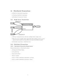
Figure 2.6.1 summarizes our discussion of SVD thus far.


A 

solutions of 

A ⋅ x = d 

null 

space 

of A 

SVD solution of 

A ⋅ x = d 

x 

solutions of 

A ⋅ x = c′ 

A ⋅ x = b 

(a) 

SVD “solution” 

of A ⋅ x = c 

(b) 

range of A 

Figure 2.6.1. (a) A nonsingular matrix A maps a vector space into one of the same dimension. The 

vector x is mapped into b, so that x satisfies the equation A · x = b. (b) A singular matrix A maps a 

vector space into one of lower dimensionality, here a plane into a line, called the “range” of A. The 

“nullspace” of A is mapped to zero. The solutions of A · x = d consist of any one particular solution plus 

any vector in the nullspace, here forming a line parallel to the nullspace. Singular value decomposition 

(SVD) selects the particular solution closest to zero, as shown. The point c lies outside of the range 

of A, soA · x = c has no solution. SVD finds the least-squares best compromise solution, namely a 

solution of A · x = c ′ , as shown. 

In the discussion since equation (2.6.6), we have been pretending that a matrix 

either is singular or else isn’t. That is of course true analytically. Numerically, 

however, the far more common situation is that some of the w j ’s are very small 

but nonzero, so that the matrix is ill-conditioned. In that case, the direct solution 

methods of LU decomposition or Gaussian elimination may actually give a formal 

solution to the set of equations (that is, a zero pivot may not be encountered); but 

the solution vector may have wildly large components whose algebraic cancellation, 

when multiplying by the matrix A, may give a very poor approximation to the 

right-hand vector b. In such cases, the solution vector x obtained by zeroing the 

d 

b 

c′ 

c 







small w j ’s and then using equation (2.6.7) is very often better (in the sense of the 

residual |A · x − b| being smaller) than both the direct-method solution and the SVD 

solution where the small w j ’s are left nonzero. 

It may seem paradoxical that this can be so, since zeroing a singular value 

corresponds to throwing away one linear combination of the set of equations that 

we are trying to solve. The resolution of the paradox is that we are throwing away 

precisely a combination of equations that is so corrupted by roundoff error as to be at 

best useless; usually it is worse than useless since it “pulls” the solution vector way 

off towards infinity along some direction that is almost a nullspace vector. In doing 

this, it compounds the roundoff problem and makes the residual |A · x − b| larger. 

SVD cannot be applied blindly, then. You have to exercise some discretion in 

deciding at what threshold to zero the small w j ’s, and/or you have to have some idea 

what size of computed residual |A · x − b| is acceptable. 

As an example, here is a “backsubstitution” routine svbksb for evaluating 

equation (2.6.7) and obtaining a solution vector x from a right-hand side b, given 

that the SVD of a matrix A has already been calculated by a call to svdcmp. Note 

that this routine presumes that you have already zeroed the small w j ’s. It does not 

do this for you. If you haven’t zeroed the small w j ’s, then this routine is just as 

ill-conditioned as any direct method, and you are misusing SVD. 

#include "nrutil.h" 

void svbksb(float **u, float w[], float **v, int m, int n, float b[], float x[]) 

Solves A·X = B for a vector X, whereA is specified by the arrays u[1..m][1..n], w[1..n], 

v[1..n][1..n] as returned by svdcmp. m and n are the dimensions of a, and will be equal for 

square matrices. b[1..m] is the input right-hand side. x[1..n] is the output solution vector. 

No input quantities are destroyed, so the routine may be called sequentially with different b’s. 

{ 

int jj,j,i; 

float s,*tmp; 

} 

tmp=vector(1,n); 

for (j=1;j


#define N ... 

float wmax,wmin,**a,**u,*w,**v,*b,*x; 

int i,j; 

... 

for(i=1;i


given by (2.6.7), which, with nonsquare matrices, looks like this, 

⎛ ⎞ ⎛ 

⎜ 

⎝ x ⎟ 

⎠ = ⎜ 

⎝ 

V 

⎞ ⎛ ⎞ ⎛ 

⎞ 

⎟ 

⎠ · 

⎜ 

⎝ diag(1/w j) ⎟ 

⎠ · 

⎜ 

⎝ U T ⎟ 

⎠ · 

b 

⎜ ⎟ 

⎝ ⎠ 

(2.6.12) 

In general, the matrix W will not be singular, and no w j ’s will need to be 

set to zero. Occasionally, however, there might be column degeneracies in A. In 

this case you will need to zero some small w j values after all. The corresponding 

column in V gives the linear combination of x’s that is then ill-determined even by 

the supposedly overdetermined set. 

Sometimes, although you do not need to zero any w j ’s for computational 

reasons, you may nevertheless want to take note of any that are unusually small: 

Their correspondingcolumns in V are linear combinations of x’s which are insensitive 

to your data. In fact, you may then wish to zero these w j ’s, to reduce the number of 

free parameters in the fit. These matters are discussed more fully in Chapter 15. 

Constructing an Orthonormal Basis 

Suppose that you have N vectors in an M-dimensional vector space, with 

N ≤ M. Then the N vectors span some subspace of the full vector space. 

Often you want to construct an orthonormal set of N vectors that span the same 

subspace. The textbook way to do this is by Gram-Schmidt orthogonalization, 

starting with one vector and then expanding the subspace one dimension at a 

time. Numerically, however, because of the build-up of roundoff errors, naive 

Gram-Schmidt orthogonalization is terrible. 

The right way to construct an orthonormal basis for a subspace is by SVD: 

Form an M × N matrix A whose N columns are your vectors. Run the matrix 

through svdcmp. The columns of the matrix U (which in fact replaces A on output 

from svdcmp) are your desired orthonormal basis vectors. 

You might also want to check the output w j ’s for zero values. If any occur, 

then the spanned subspace was not, in fact, N dimensional; the columns of U 

corresponding to zero w j ’s should be discarded from the orthonormal basis set. 

(QR factorization, discussed in §2.10, also constructs an orthonormal basis, 

see [5].) 

Approximation of Matrices 

Note that equation (2.6.1) can be rewritten to express any matrix A ij as a sum 

of outer products of columns of U and rows of V T , with the “weighting factors” 

being the singular values w j , 

N∑ 

A ij = w k U ik V jk (2.6.13) 

k=1 

⎛ 

⎞ 







If you ever encounter a situation where most of the singular values w j of a 

matrix A are very small, then A will be well-approximated by only a few terms in the 

sum (2.6.13). This means that you have to store only a few columns of U and V (the 

same k ones) and you will be able to recover, with good accuracy, the whole matrix. 

Note also that it is very efficient to multiply such an approximated matrix by a 

vector x: You just dot x with each of the stored columns of V, multiply the resulting 

scalar by the corresponding w k , and accumulate that multiple of the corresponding 

column of U. If your matrix is approximated by a small number K of singular 

values, then this computation of A · x takes only about K(M + N) multiplications, 

instead of MN for the full matrix. 

SVD Algorithm 

Here is the algorithm for constructing the singular value decomposition of any 

matrix. See §11.2–§11.3, and also [4-5], for discussion relating to the underlying 

method. 

#include 

#include "nrutil.h" 

void svdcmp(float **a, int m, int n, float w[], float **v) 

Given a matrix a[1..m][1..n], this routine computes its singular value decomposition, A = 

U ·W ·V T . The matrix U replaces a on output. The diagonal matrix of singular values W is output 

as a vector w[1..n]. The matrix V (not the transpose V T ) is output as v[1..n][1..n]. 

{ 

float pythag(float a, float b); 

int flag,i,its,j,jj,k,l,nm; 

float anorm,c,f,g,h,s,scale,x,y,z,*rv1; 

rv1=vector(1,n); 

g=scale=anorm=0.0; 

Householder reduction to bidiagonal form. 

for (i=1;i


for (k=l;k


f=s*rv1[i]; 

rv1[i]=c*rv1[i]; 

if ((float)(fabs(f)+anorm) == anorm) break; 

g=w[i]; 

h=pythag(f,g); 

w[i]=h; 

h=1.0/h; 

c=g*h; 

s = -f*h; 

for (j=1;j


} 

for (jj=1;jj absb) return absa*sqrt(1.0+SQR(absb/absa)); 

else return (absb == 0.0 0.0 : absb*sqrt(1.0+SQR(absa/absb))); 

} 

(Double precision versions of svdcmp, svbksb, and pythag, named dsvdcmp, 

dsvbksb, and dpythag, are used by the routine ratlsq in §5.13. You can easily 

make the conversions, or else get the converted routines from the Numerical Recipes 

diskette.) 

CITED REFERENCES AND FURTHER READING: 

Golub, G.H., and Van Loan, C.F. 1989, Matrix Computations, 2nd ed. (Baltimore: Johns Hopkins 

University Press), §8.3 and Chapter 12. 

Lawson, C.L., and Hanson, R. 1974, Solving Least Squares Problems (Englewood Cliffs, NJ: 

Prentice-Hall), Chapter 18. 

Forsythe, G.E., Malcolm, M.A., and Moler, C.B. 1977, Computer Methods for Mathematical 

Computations (Englewood Cliffs, NJ: Prentice-Hall), Chapter 9. [1] 

Wilkinson, J.H., and Reinsch, C. 1971, Linear Algebra, vol. II of Handbook for Automatic Computation 

(New York: Springer-Verlag), Chapter I.10 by G.H. Golub and C. Reinsch. [2] 

Dongarra, J.J., et al. 1979, LINPACK User’s Guide (Philadelphia: S.I.A.M.), Chapter 11. [3] 

Smith, B.T., et al. 1976, Matrix Eigensystem Routines — EISPACK Guide, 2nd ed., vol. 6 of 

Lecture Notes in Computer Science (New York: Springer-Verlag). 

Stoer, J., and Bulirsch, R. 1980, Introduction to Numerical Analysis (New York: Springer-Verlag), 

§6.7. [4] 

Golub, G.H., and Van Loan, C.F. 1989, Matrix Computations, 2nd ed. (Baltimore: Johns Hopkins 

University Press), §5.2.6. [5] 






2.7 Sparse Linear Systems 71 

2.7 Sparse Linear Systems 

A system of linear equations is called sparse if only a relatively small number 

of its matrix elements a ij are nonzero. It is wasteful to use general methods of 

linear algebra on such problems, because most of the O(N 3 ) arithmetic operations 

devoted to solving the set of equations or inverting the matrix involve zero operands. 

Furthermore, you might wish to work problems so large as to tax your available 

memory space, and it is wasteful to reserve storage for unfruitful zero elements. 

Note that there are two distinct (and not always compatible) goals for any sparse 

matrix method: saving time and/or saving space. 

We have already considered one archetypal sparse form in §2.4, the band 

diagonal matrix. In the tridiagonal case, e.g., we saw that it was possible to save 

both time (order N instead of N 3 ) and space (order N instead of N 2 ). The 

method of solution was not different in principle from the general method of LU 

decomposition; it was just applied cleverly, and with due attention to the bookkeeping 

of zero elements. Many practical schemes for dealing with sparse problems have this 

same character. They are fundamentally decomposition schemes, or else elimination 

schemes akin to Gauss-Jordan, but carefully optimized so as to minimize the number 

of so-called fill-ins, initially zero elements which must become nonzero during the 

solution process, and for which storage must be reserved. 

Direct methods for solving sparse equations, then, depend crucially on the 

precise pattern of sparsity of the matrix. Patterns that occur frequently, or that are 

useful as way-stations in the reduction of more general forms, already have special 

names and special methods of solution. We do not have space here for any detailed 

review of these. References listed at the end of this section will furnish you with an 

“in” to the specialized literature, and the following list of buzz words (and Figure 

2.7.1) will at least let you hold your own at cocktail parties: 

• tridiagonal 

• band diagonal (or banded) with bandwidth M 

• band triangular 

• block diagonal 

• block tridiagonal 

• block triangular 

• cyclic banded 

• singly (or doubly) bordered block diagonal 

• singly (or doubly) bordered block triangular 

• singly (or doubly) bordered band diagonal 

• singly (or doubly) bordered band triangular 

• other (!) 

You should also be aware of some of the special sparse forms that occur in the 

solution of partial differential equations in two or more dimensions. See Chapter 19. 





http://www.nr.com or call 1-800-872-7423 (North America only), or send email to directcustserv@cambridge.org (outside North America). 

If your particular pattern of sparsity is not a simple one, then you may wish to 

try an analyze/factorize/operate package, which automates the procedure of figuring 

out how fill-ins are to be minimized. The analyze stage is done once only for each 

pattern of sparsity. The factorize stage is done once for each particular matrix that 

fits the pattern. The operate stage is performed once for each right-hand side to

SVD-Numerical Recipe in C - 3MAP

Create successful ePaper yourself

Delete template?

Save as template?