11.1 Jacobi Transformations of a Symmetric Matrix

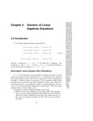
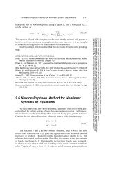
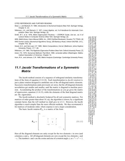
11.1 Jacobi Transformations of a Symmetric Matrix 463CITED REFERENCES AND FURTHER READING:Stoer, J., and Bulirsch, R. 1980, Introduction to Numerical Analysis (New York: Springer-Verlag),Chapter 6. [1]Wilkinson, J.H., and Reinsch, C. 1971, Linear Algebra, vol. II of Handbook for Automatic Computation(New York: Springer-Verlag). [2]Smith, B.T., et al. 1976, Matrix Eigensystem Routines — EISPACK Guide, 2nd ed., vol. 6 ofLecture Notes in Computer Science (New York: Springer-Verlag). [3]IMSL Math/Library Users Manual (IMSL Inc., 2500 CityWest Boulevard, Houston TX 77042). [4]NAG Fortran Library (Numerical Algorithms Group, 256 Banbury Road, Oxford OX27DE, U.K.),Chapter F02. [5]Golub, G.H., and Van Loan, C.F. 1989, Matrix Computations, 2nd ed. (Baltimore: Johns HopkinsUniversity Press), §7.7. [6]Wilkinson, J.H. 1965, The Algebraic Eigenvalue Problem (New York: Oxford University Press). [7]Acton, F.S. 1970, Numerical Methods That Work; 1990, corrected edition (Washington: MathematicalAssociation of America), Chapter 13.Horn, R.A., and Johnson, C.R. 1985, Matrix Analysis (Cambridge: Cambridge University Press).11.1 Jacobi Transformations of a SymmetricMatrixThe Jacobi method consists of a sequence of orthogonal similarity transformationsof the form of equation (11.0.14). Each transformation (a Jacobi rotation) isjust a plane rotation designed to annihilate one of the off-diagonal matrix elements.Successive transformations undo previously set zeros, but the off-diagonal elementsnevertheless get smaller and smaller, until the matrix is diagonal to machine precision.Accumulating the product of the transformations as you go gives the matrixof eigenvectors, equation (11.0.15), while the elements of the final diagonal matrixare the eigenvalues.The Jacobi method is absolutely foolproof for all real symmetric matrices. Formatrices of order greater than about 10, say, the algorithm is slower, by a significantconstant factor, than the QR method we shall give in §11.3. However, the Jacobialgorithm is much simpler than the more efficient methods. We thus recommend itfor matrices of moderate order, where expense is not a major consideration.The basic Jacobi rotation P pq is a matrix of the form⎡1P pq =⎢⎣···c ··· s. .. 1 .−s ··· c···⎤⎥⎦1(11.1.1)Sample page from NUMERICAL RECIPES IN C: THE ART OF SCIENTIFIC COMPUTING (ISBN 0-521-43108-5)Copyright (C) 1988-1992 by Cambridge University Press. Programs Copyright (C) 1988-1992 by Numerical Recipes Software.Permission is granted for internet users to make one paper copy for their own personal use. Further reproduction, or any copying of machinereadablefiles (including this one) to any server computer, is strictly prohibited. To order Numerical Recipes books or CDROMs, visit websitehttp://www.nr.com or call 1-800-872-7423 (North America only), or send email to directcustserv@cambridge.org (outside North America).Here all the diagonal elements are unity except for the two elements c in rows (andcolumns) p and q. All off-diagonal elements are zero except the two elements s and−s. The numbers c and s are the cosine and sine of a rotation angle φ,soc 2 +s 2 =1.

464 Chapter 11. EigensystemsA plane rotation such as (11.1.1) is used to transform the matrix A according toA ′ = P T pq · A · P pq (11.1.2)Now, P T pq · A changes only rows p and q of A, while A · P pq changes only columnsp and q. Notice that the subscripts p and q do not denote components of P pq ,butrather label which kind of rotation the matrix is, i.e., which rows and columns itaffects. Thus the changed elements of A in (11.1.2) are only in the p and q rowsand columns indicated below:⎡··· a ′ 1p ··· a ′ ⎤1q ···. . . .a ′ p1 ··· a ′ pp ··· a ′ pq ··· a ′ pnA ′ =. . . .a ′ q1 ··· a ′ qp ··· a ′ qq ··· a ′ qn⎢⎣ . . . . ⎥. . . .⎦··· a ′ np ··· a ′ nq ···(11.1.3)Multiplying out equation (11.1.2) and using the symmetry of A, we get the explicitformulasa ′ rp = ca rp − sa rqa ′ rq = ca rq + sa rpr ≠ p, r ≠ q (11.1.4)a ′ pp = c2 a pp + s 2 a qq − 2sca pq (11.1.5)a ′ qq = s2 a pp + c 2 a qq +2sca pq (11.1.6)a ′ pq =(c 2 − s 2 )a pq + sc(a pp − a qq ) (11.1.7)The idea of the Jacobi method is to try to zero the off-diagonal elements by aseries of plane rotations. Accordingly, to set a ′ pq =0, equation (11.1.7) gives thefollowing expression for the rotation angle φθ ≡ cot 2φ ≡ c2 − s 22scIf we let t ≡ s/c, the definition of θ can be rewritten= a qq − a pp2a pq(11.1.8)t 2 +2tθ − 1=0 (11.1.9)The smaller root of this equation corresponds to a rotation angle less than π/4in magnitude; this choice at each stage gives the most stable reduction. Using theform of the quadratic formula with the discriminant in the denominator, we canwrite this smaller root asSample page from NUMERICAL RECIPES IN C: THE ART OF SCIENTIFIC COMPUTING (ISBN 0-521-43108-5)Copyright (C) 1988-1992 by Cambridge University Press. Programs Copyright (C) 1988-1992 by Numerical Recipes Software.Permission is granted for internet users to make one paper copy for their own personal use. Further reproduction, or any copying of machinereadablefiles (including this one) to any server computer, is strictly prohibited. To order Numerical Recipes books or CDROMs, visit websitehttp://www.nr.com or call 1-800-872-7423 (North America only), or send email to directcustserv@cambridge.org (outside North America).sgn(θ)t =|θ| + √ θ 2 +1(11.1.10)

11.1 Jacobi Transformations of a Symmetric Matrix 465If θ is so large that θ 2 would overflow on the computer, we set t =1/(2θ).now follows thatItc =1√t2 +1(11.1.11)s = tc (11.1.12)When we actually use equations (11.1.4)–(11.1.7) numerically, we rewrite themto minimize roundoff error. Equation (11.1.7) is replaced bya ′ pq =0 (11.1.13)The idea in the remaining equations is to set the new quantity equal to the oldquantity plus a small correction. Thus we can use (11.1.7) and (11.1.13) to eliminatea qq from (11.1.5), givingSimilarly,where τ (= tan φ/2) is defined bya ′ pp = a pp − ta pq (11.1.14)a ′ qq = a qq + ta pq (11.1.15)a ′ rp = a rp − s(a rq + τa rp ) (11.1.16)a ′ rq = a rq + s(a rp − τa rq ) (11.1.17)τ ≡s1+c(11.1.18)One can see the convergence of the Jacobi method by considering the sum ofthe squares of the off-diagonal elementsEquations (11.1.4)–(11.1.7) imply thatS = ∑ |a rs | 2 (11.1.19)r≠sS ′ = S − 2|a pq | 2 (11.1.20)(Since the transformation is orthogonal, the sum of the squares of the diagonalelements increases correspondingly by 2|a pq | 2 .) The sequence of S’s thus decreasesmonotonically. Since the sequence is bounded below by zero, and since we canchoose a pq to be whatever element we want, the sequence can be made to convergeto zero.Sample page from NUMERICAL RECIPES IN C: THE ART OF SCIENTIFIC COMPUTING (ISBN 0-521-43108-5)Copyright (C) 1988-1992 by Cambridge University Press. Programs Copyright (C) 1988-1992 by Numerical Recipes Software.Permission is granted for internet users to make one paper copy for their own personal use. Further reproduction, or any copying of machinereadablefiles (including this one) to any server computer, is strictly prohibited. To order Numerical Recipes books or CDROMs, visit websitehttp://www.nr.com or call 1-800-872-7423 (North America only), or send email to directcustserv@cambridge.org (outside North America).Eventually one obtains a matrix D that is diagonal to machine precision. Thediagonal elements give the eigenvalues of the original matrix A, sinceD = V T · A · V (11.1.21)

466 Chapter 11. EigensystemswhereV = P 1 · P 2 · P 3 ··· (11.1.22)the P i ’s being the successive Jacobi rotation matrices. The columns of V are theeigenvectors (since A · V = V · D). They can be computed by applyingV ′ = V · P i (11.1.23)at each stage of calculation, where initially V is the identity matrix.equation (11.1.23) isv ′ rs = v rs (s ≠ p, s ≠ q)In detail,v ′ rp = cv rp − sv rqv ′ rq = sv rp + cv rq(11.1.24)We rewrite these equations in terms of τ as in equations (11.1.16) and (11.1.17)to minimize roundoff.The only remaining question is the strategy one should adopt for the order inwhich the elements are to be annihilated. Jacobi’s original algorithm of 1846 searchedthe whole upper triangle at each stage and set the largest off-diagonal element to zero.This is a reasonable strategy for hand calculation, but it is prohibitive on a computersince the search alone makes each Jacobi rotation a process of order N 2 instead of N.A better strategy for our purposes is the cyclic Jacobi method, where oneannihilates elements in strict order. For example, one can simply proceed downthe rows: P 12 , P 13 , ..., P 1n ; then P 23 , P 24 , etc. One can show that convergenceis generally quadratic for both the original or the cyclic Jacobi methods, fornondegenerate eigenvalues. One such set of n(n − 1)/2 Jacobi rotations is calleda sweep.The program below, based on the implementations in [1,2], uses two furtherrefinements:• In the first three sweeps, we carry out the pq rotation only if |a pq | >ɛfor some threshold valuewhere S 0 is the sum of the off-diagonal moduli,ɛ = 1 S 05 n 2 (11.1.25)S 0 = ∑ |a rs | (11.1.26)r

11.1 Jacobi Transformations of a Symmetric Matrix 467In the following routine the n×n symmetric matrix a is stored as a[1..n][1..n]. On output, the superdiagonal elements of a are destroyed, but the diagonaland subdiagonal are unchanged and give full information on the original symmetricmatrix a. The vector d[1..n] returns the eigenvalues of a. During the computation,it contains the current diagonal of a. The matrix v[1..n][1..n] outputs thenormalized eigenvector belonging to d[k] in its kth column. The parameter nrot isthe number of Jacobi rotations that were needed to achieve convergence.Typical matrices require 6 to 10 sweeps to achieve convergence, or 3n 2 to 5n 2Jacobi rotations. Each rotation requires of order 4n operations, each consistingof a multiply and an add, so the total labor is of order 12n 3 to 20n 3 operations.Calculation of the eigenvectors as well as the eigenvalues changes the operationcount from 4n to 6n per rotation, which is only a 50 percent overhead.#include #include "nrutil.h"#define ROTATE(a,i,j,k,l) g=a[i][j];h=a[k][l];a[i][j]=g-s*(h+g*tau);\a[k][l]=h+s*(g-h*tau);void jacobi(float **a, int n, float d[], float **v, int *nrot)Computes all eigenvalues and eigenvectors of a real symmetric matrix a[1..n][1..n]. Onoutput, elements of a above the diagonal are destroyed. d[1..n] returns the eigenvalues of a.v[1..n][1..n] is a matrix whose columns contain, on output, the normalized eigenvectors ofa. nrot returns the number of Jacobi rotations that were required.{int j,iq,ip,i;float tresh,theta,tau,t,sm,s,h,g,c,*b,*z;b=vector(1,n);z=vector(1,n);for (ip=1;ip

468 Chapter 11. Eigensystems}else if (fabs(a[ip][iq]) > tresh) {h=d[iq]-d[ip];if ((float)(fabs(h)+g) == (float)fabs(h))t=(a[ip][iq])/h;t =1/(2θ)else {theta=0.5*h/(a[ip][iq]); Equation (11.1.10).t=1.0/(fabs(theta)+sqrt(1.0+theta*theta));if (theta < 0.0) t = -t;}c=1.0/sqrt(1+t*t);s=t*c;tau=s/(1.0+c);h=t*a[ip][iq];z[ip] -= h;z[iq] += h;d[ip] -= h;d[iq] += h;a[ip][iq]=0.0;for (j=1;j

11.2 Reduction of a Symmetric Matrix to Tridiagonal Form 469}}for (j=i+1;j= p) p=d[k=j];if (k != i) {d[k]=d[i];d[i]=p;for (j=1;j