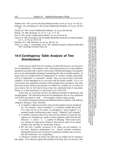
14.4 Contingency Table Analysis of Two Distributions

630 Chapter 14. Statistical Description of Datafirst variable x taking on its ith value, and the second variable y taking on its jthvalue. Let N denote the total number of events, the sum of all the N ij ’s. Let N i·denote the number of events for which the first variable x takes on its ith valueregardless of the value of y; N·j is the number of events with the jth value of yregardless of x. So we haveN i· = ∑ jN = ∑ iN ijN i· = ∑ jN·j = ∑ iN ijN·j(14.4.1)N·j and N i· are sometimes called the row and column totals or marginals, but wewill use these terms cautiously since we can never keep straight which are the rowsand which are the columns!The null hypothesis is that the two variables x and y have no association. In thiscase, the probability of a particular value of x given a particular value of y shouldbe the same as the probability of that value of x regardless of y. Therefore, in thenull hypothesis, the expected number for any N ij , which we will denote n ij , can becalculated from only the row and column totals,n ijN·j= N i·Nwhich impliesn ij = N i·N·jN(14.4.2)Notice that if a column or row total is zero, then the expected number for all theentries in that column or row is also zero; in that case, the never-occurring bin of xor y should simply be removed from the analysis.The chi-square statistic is now given by equation (14.3.1), which, in the presentcase, is summed over all entries in the table,χ 2 = ∑ i,j(N ij − n ij ) 2n ij(14.4.3)The number of degrees of freedom is equal to the number of entries in the table(product of its row size and column size) minus the number of constraints that havearisen from our use of the data themselves to determine the n ij . Each row total andcolumn total is a constraint, except that this overcounts by one, since the total of thecolumn totals and the total of the row totals both equal N, the total number of datapoints. Therefore, if the table is of size I by J, the number of degrees of freedom isIJ − I − J +1. Equation (14.4.3), along with the chi-square probability function(§6.2), now give the significance of an association between the variables x and y.Suppose there is a significant association. How do we quantify its strength, sothat (e.g.) we can compare the strength of one association with another? The ideahere is to find some reparametrization of χ 2 which maps it into some convenientinterval, like 0 to 1, where the result is not dependent on the quantity of data that wehappen to sample, but rather depends only on the underlying population from whichthe data were drawn. There are several different ways of doing this. Two of the morecommon are called Cramer’s V and the contingency coefficient C.Sample page from NUMERICAL RECIPES IN C: THE ART OF SCIENTIFIC COMPUTING (ISBN 0-521-43108-5)Copyright (C) 1988-1992 by Cambridge University Press. Programs Copyright (C) 1988-1992 by Numerical Recipes Software.Permission is granted for internet users to make one paper copy for their own personal use. Further reproduction, or any copying of machinereadablefiles (including this one) to any server computer, is strictly prohibited. To order Numerical Recipes books or CDROMs, visit websitehttp://www.nr.com or call 1-800-872-7423 (North America only), or send email to directcustserv@cambridge.org (outside North America).

14.4 Contingency Table Analysis of Two Distributions 631The formula for Cramer’s V is√χV =2N min (I − 1,J − 1)(14.4.4)where I and J are again the numbers of rows and columns, and N is the totalnumber of events. Cramer’s V has the pleasant property that it lies between zeroand one inclusive, equals zero when there is no association, and equals one onlywhen the association is perfect: All the events in any row lie in one unique column,and vice versa. (In chess parlance, no two rooks, placed on a nonzero table entry,can capture each other.)In the case of I = J =2, Cramer’s V is also referred to as the phi statistic.The contingency coefficient C is defined as√χC =2χ 2 + N(14.4.5)It also lies between zero and one, but (as is apparent from the formula) it can neverachieve the upper limit. While it can be used to compare the strength of associationof two tables with the same I and J, its upper limit depends on I and J. Thereforeit can never be used to compare tables of different sizes.The trouble with both Cramer’s V and the contingency coefficient C is that, whenthey take on values in between their extremes, there is no very direct interpretationof what that value means. For example, you are in Las Vegas, and a friend tells youthat there is a small, but significant, association between the color of a croupier’seyes and the occurrence of red and black on his roulette wheel. Cramer’s V is about0.028, your friend tells you. You know what the usual odds against you are (becauseof the green zero and double zero on the wheel). Is this association sufficient foryou to make money? Don’t ask us!#include #include "nrutil.h"#define TINY 1.0e-30A small number.void cntab1(int **nn, int ni, int nj, float *chisq, float *df, float *prob,float *cramrv, float *ccc)Given a two-dimensional contingency table in the form of an integer array nn[1..ni][1..nj],this routine returns the chi-square chisq, the number of degrees of freedom df, the significancelevel prob (small values indicating a significant association), and two measures of association,Cramer’s V (cramrv) and the contingency coefficient C (ccc).{float gammq(float a, float x);int nnj,nni,j,i,minij;float sum=0.0,expctd,*sumi,*sumj,temp;sumi=vector(1,ni);sumj=vector(1,nj);nni=ni;nnj=nj;for (i=1;i

632 Chapter 14. Statistical Description of Data}}if (sumi[i] == 0.0) --nni; Eliminate any zero rows by reducing the number.}for (j=1;j

14.4 Contingency Table Analysis of Two Distributions 633H takes on its maximum value when all the p i ’s are equal, in which case the questionis sure to eliminate all but a fraction 1/I of the remaining possibilities.The value H is conventionally termed the entropy of the distribution given bythe p i ’s, a terminology borrowed from statistical physics.So far we have said nothing about the association of two variables; but supposewe are deciding what question to ask next in the game and have to choose betweentwo candidates, or possibly want to ask both in one order or another. Suppose thatone question, x, has I possible answers, labeled by i, and that the other question,y, asJ possible answers, labeled by j. Then the possible outcomes of asking bothquestions form a contingency table whose entries N ij , when normalized by dividingby the total number of remaining possibilities N, give all the information about thep’s. In particular, we can make contact with the notation (14.4.1) by identifyingp ij = N ijNp i· = N i·Np·j = N·jN(outcomes of question x alone)(outcomes of question y alone)The entropies of the questions x and y are, respectively,H(x) =− ∑ ip i· ln p i·The entropy of the two questions together isH(x, y) =− ∑ i,jH(y) =− ∑ j(14.4.8)p·j ln p·j (14.4.9)p ij ln p ij (14.4.10)Now what is the entropy of the question y given x (that is, if x is asked first)?It is the expectation value over the answers to x of the entropy of the restrictedy distribution that lies in a single column of the contingency table (correspondingto the x answer):H(y|x) =− ∑ ip i·∑jp ijp i·ln p ijp i·= − ∑ i,jCorrespondingly, the entropy of x given y isH(x|y) =− ∑ jp·j∑ip ijp·jln p ijp·j= − ∑ i,jp ij ln p ijp i·(14.4.11)p ij ln p ijp·j(14.4.12)Sample page from NUMERICAL RECIPES IN C: THE ART OF SCIENTIFIC COMPUTING (ISBN 0-521-43108-5)Copyright (C) 1988-1992 by Cambridge University Press. Programs Copyright (C) 1988-1992 by Numerical Recipes Software.Permission is granted for internet users to make one paper copy for their own personal use. Further reproduction, or any copying of machinereadablefiles (including this one) to any server computer, is strictly prohibited. To order Numerical Recipes books or CDROMs, visit websitehttp://www.nr.com or call 1-800-872-7423 (North America only), or send email to directcustserv@cambridge.org (outside North America).We can readily prove that the entropy of y given x is never more than theentropy of y alone, i.e., that asking x first can only reduce the usefulness of asking

634 Chapter 14. Statistical Description of Datay (in which case the two variables are associated!):H(y|x) − H(y) =− ∑ i,jp ij ln p ij/p i·p·j= ∑ i,j≤ ∑ i,j= ∑ i,jp ij ln p·jp i·p ijp ij(p·j p i·p ij− 1p i·p·j − ∑ i,j=1− 1=0p ij)(14.4.13)where the inequality follows from the factln w ≤ w − 1 (14.4.14)We now have everything we need to define a measure of the “dependency” of yon x, that is to say a measure of association. This measure is sometimes called theuncertainty coefficient of y. We will denote it as U(y|x),H(y) − H(y|x)U(y|x) ≡ (14.4.15)H(y)This measure lies between zero and one, with the value 0 indicating that x and yhave no association, the value 1 indicating that knowledge of x completely predictsy. For in-between values, U(y|x) gives the fraction of y’s entropy H(y) that islost if x is already known (i.e., that is redundant with the information in x). In ourgame of “twenty questions,” U(y|x) is the fractional loss in the utility of questiony if question x is to be asked first.If we wish to view x as the dependent variable, y as the independent one, theninterchanging x and y we can of course define the dependency of x on y,H(x) − H(x|y)U(x|y) ≡ (14.4.16)H(x)If we want to treat x and y symmetrically, then the useful combination turnsout to be[ ]H(y)+H(x) − H(x, y)U(x, y) ≡ 2(14.4.17)H(x)+H(y)If the two variables are completely independent, then H(x, y) =H(x)+H(y), so(14.4.17) vanishes. If the two variables are completely dependent, then H(x) =H(y) =H(x, y), so (14.4.16) equals unity. In fact, you can use the identities (easilyproved from equations 14.4.9–14.4.12)H(x, y) =H(x)+H(y|x) =H(y)+H(x|y) (14.4.18)to show thatU(x, y) = H(x)U(x|y)+H(y)U(y|x)(14.4.19)H(x)+H(y)i.e., that the symmetrical measure is just a weighted average of the two asymmetricalmeasures (14.4.15) and (14.4.16),weighted by the entropy of each variable separately.Here is a program for computing all the quantities discussed, H(x), H(y),H(x|y), H(y|x), H(x, y), U(x|y), U(y|x), and U(x, y):Sample page from NUMERICAL RECIPES IN C: THE ART OF SCIENTIFIC COMPUTING (ISBN 0-521-43108-5)Copyright (C) 1988-1992 by Cambridge University Press. Programs Copyright (C) 1988-1992 by Numerical Recipes Software.Permission is granted for internet users to make one paper copy for their own personal use. Further reproduction, or any copying of machinereadablefiles (including this one) to any server computer, is strictly prohibited. To order Numerical Recipes books or CDROMs, visit websitehttp://www.nr.com or call 1-800-872-7423 (North America only), or send email to directcustserv@cambridge.org (outside North America).

14.4 Contingency Table Analysis of Two Distributions 635#include #include "nrutil.h"#define TINY 1.0e-30A small number.void cntab2(int **nn, int ni, int nj, float *h, float *hx, float *hy,float *hygx, float *hxgy, float *uygx, float *uxgy, float *uxy)Given a two-dimensional contingency table in the form of an integer array nn[i][j], whereilabels the x variable and ranges from 1 to ni, j labels the y variable and ranges from 1 to nj,this routine returns the entropy h of the whole table, the entropy hx of the x distribution, theentropy hy of the y distribution, the entropy hygx of y given x, theentropyhxgy of x given y,the dependency uygx of y on x (eq. 14.4.15), the dependency uxgy of x on y (eq. 14.4.16),and the symmetrical dependency uxy (eq. 14.4.17).{int i,j;float sum=0.0,p,*sumi,*sumj;sumi=vector(1,ni);sumj=vector(1,nj);for (i=1;i

636 Chapter 14. Statistical Description of DataNorusis, M.J. 1982, SPSS Introductory Guide: Basic Statistics and Operations; and 1985, SPSS-X Advanced Statistics Guide (New York: McGraw-Hill).Fano, R.M. 1961, Transmission of Information (New York: Wiley and MIT Press), Chapter 2.14.5 Linear CorrelationWe next turn to measures of association between variables that are ordinalor continuous, rather than nominal. Most widely used is the linear correlationcoefficient. For pairs of quantities (x i ,y i ), i =1,...,N, the linear correlationcoefficient r (also called the product-moment correlation coefficient, or Pearson’sr) is given by the formula∑(x i − x)(y i − y)ir = √ ∑ √ ∑ (14.5.1)(x i − x) 2 (y i − y) 2iiwhere, as usual, x is the mean of the x i ’s, y is the mean of the y i ’s.The value of r lies between −1 and 1, inclusive. It takes on a value of 1, termed“complete positive correlation,” when the data points lie on a perfect straight linewith positive slope, with x and y increasing together. The value 1 holds independentof the magnitude of the slope. If the data points lie on a perfect straight line withnegative slope, y decreasing as x increases, then r has the value −1; this is called“complete negative correlation.” A value of r near zero indicates that the variablesx and y are uncorrelated.When a correlation is known to be significant, r is one conventional way ofsummarizing its strength. In fact, the value of r can be translated into a statementabout what residuals (root mean square deviations) are to be expected if the data arefitted to a straight line by the least-squares method (see §15.2, especially equations15.2.13 – 15.2.14). Unfortunately, r is a rather poor statistic for deciding whetheran observed correlation is statistically significant, and/or whether one observedcorrelation is significantly stronger than another. The reason is that r is ignorant ofthe individual distributions of x and y, so there is no universal way to compute itsdistribution in the case of the null hypothesis.About the only general statement that can be made is this: If the null hypothesisis that x and y are uncorrelated, and if the distributions for x and y each haveenough convergent moments (“tails” die off sufficiently rapidly), and if N is large(typically > 500), then r is distributed approximately normally, with a mean of zeroand a standard deviation of 1/ √ N. In that case, the (double-sided) significance ofthe correlation, that is, the probability that |r| should be larger than its observedvalue in the null hypothesis, is(|r| √ )Nerfc √ (14.5.2)2Sample page from NUMERICAL RECIPES IN C: THE ART OF SCIENTIFIC COMPUTING (ISBN 0-521-43108-5)Copyright (C) 1988-1992 by Cambridge University Press. Programs Copyright (C) 1988-1992 by Numerical Recipes Software.Permission is granted for internet users to make one paper copy for their own personal use. Further reproduction, or any copying of machinereadablefiles (including this one) to any server computer, is strictly prohibited. To order Numerical Recipes books or CDROMs, visit websitehttp://www.nr.com or call 1-800-872-7423 (North America only), or send email to directcustserv@cambridge.org (outside North America).where erfc(x) is the complementary error function, equation (6.2.8), computed bythe routines erffc or erfcc of §6.2. A small value of (14.5.2) indicates that the