Chapter 2. Solution of Linear Algebraic Equations 2.0 Introduction

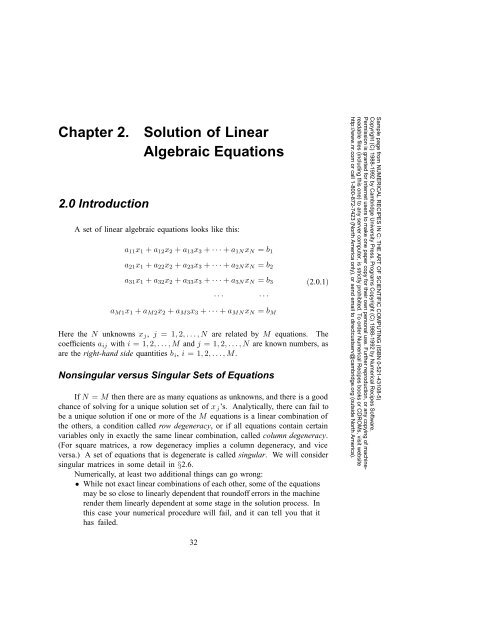
Chapter 2.2.0 IntroductionSolution of LinearAlgebraic EquationsA set of linear algebraic equations looks like this:a 11 x 1 + a 12 x 2 + a 13 x 3 + ···+ a 1N x N = b 1a 21 x 1 + a 22 x 2 + a 23 x 3 + ···+ a 2N x N = b 2a 31 x 1 + a 32 x 2 + a 33 x 3 + ···+ a 3N x N = b 3 (2.0.1)··· ···a M1 x 1 + a M2 x 2 + a M3 x 3 + ···+ a MN x N = b MHere the N unknowns x j , j =1, 2,...,N are related by M equations. Thecoefficients a ij with i =1, 2,...,M and j =1, 2,...,N are known numbers, asare the right-hand side quantities b i , i =1, 2,...,M.Nonsingular versus Singular Sets of EquationsIf N = M then there are as many equations as unknowns, and there is a goodchance of solving for a unique solution set of x j ’s. Analytically, there can fail tobe a unique solution if one or more of the M equations is a linear combination ofthe others, a condition called row degeneracy, or if all equations contain certainvariables only in exactly the same linear combination, called column degeneracy.(For square matrices, a row degeneracy implies a column degeneracy, and viceversa.) A set of equations that is degenerate is called singular. We will considersingular matrices in some detail in §2.6.Numerically, at least two additional things can go wrong:• While not exact linear combinations of each other, some of the equationsmay be so close to linearly dependent that roundoff errors in the machinerender them linearly dependent at some stage in the solution process. Inthis case your numerical procedure will fail, and it can tell you that ithas failed.Sample page from NUMERICAL RECIPES IN C: THE ART OF SCIENTIFIC COMPUTING (ISBN 0-521-43108-5)Copyright (C) 1988-1992 by Cambridge University Press. Programs Copyright (C) 1988-1992 by Numerical Recipes Software.Permission is granted for internet users to make one paper copy for their own personal use. Further reproduction, or any copying of machinereadablefiles (including this one) to any server computer, is strictly prohibited. To order Numerical Recipes books or CDROMs, visit websitehttp://www.nr.com or call 1-800-872-7423 (North America only), or send email to directcustserv@cambridge.org (outside North America).32

34 Chapter 2. Solution of Linear Algebraic Equationsat this point. Occasionally it is useful to be able to peer through the veil, for exampleto pass a whole row a[i][j], j=1,...,N by the reference a[i].Tasks of Computational Linear AlgebraWe will consider the following tasks as falling in the general purview of thischapter:• Solution of the matrix equation A·x = b for an unknown vector x, where Ais a square matrix of coefficients, raised dot denotes matrix multiplication,and b is a known right-hand side vector (§2.1–§2.10).• Solution of more than one matrix equation A · x j = b j , for a set of vectorsx j , j =1, 2,..., each corresponding to a different, known right-hand sidevector b j . In this task the key simplification is that the matrix A is heldconstant, while the right-hand sides, the b’s, are changed (§2.1–§2.10).• Calculation of the matrix A −1 which is the matrix inverse of a square matrixA, i.e., A · A −1 = A −1 · A = 1, where 1 is the identity matrix (all zerosexcept for ones on the diagonal). This task is equivalent, for an N × Nmatrix A, to the previous task with N different b j ’s (j =1, 2,...,N),namely the unit vectors (b j = all zero elements except for 1 in the jthcomponent). The corresponding x’s are then the columns of the matrixinverse of A (§2.1 and §2.3).• Calculation of the determinant of a square matrix A (§2.3).If M < N, or if M = N but the equations are degenerate, then thereare effectively fewer equations than unknowns. In this case there can be either nosolution, or else more than one solution vector x. In the latter event, the solution spaceconsists of a particular solution x p added to any linear combination of (typically)N − M vectors (which are said to be in the nullspace of the matrix A). The taskof finding the solution space of A involves• Singular value decomposition of a matrix A.This subject is treated in §2.6.In the opposite case there are more equations than unknowns, M>N. Whenthis occurs there is, in general, no solution vector x to equation (2.0.1), and the setof equations is said to be overdetermined. It happens frequently, however, that thebest “compromise” solution is sought, the one that comes closest to satisfying allequations simultaneously. If closeness is defined in the least-squares sense, i.e., thatthe sum of the squares of the differences between the left- and right-hand sides ofequation (2.0.1) be minimized, then the overdetermined linear problem reduces toa (usually) solvable linear problem, called the• Linear least-squares problem.The reduced set of equations to be solved can be written as the N ×N set of equationsSample page from NUMERICAL RECIPES IN C: THE ART OF SCIENTIFIC COMPUTING (ISBN 0-521-43108-5)Copyright (C) 1988-1992 by Cambridge University Press. Programs Copyright (C) 1988-1992 by Numerical Recipes Software.Permission is granted for internet users to make one paper copy for their own personal use. Further reproduction, or any copying of machinereadablefiles (including this one) to any server computer, is strictly prohibited. To order Numerical Recipes books or CDROMs, visit websitehttp://www.nr.com or call 1-800-872-7423 (North America only), or send email to directcustserv@cambridge.org (outside North America).(A T · A) · x =(A T · b) (2.0.4)where A T denotes the transpose of the matrix A. Equations (2.0.4) are called thenormal equations of the linear least-squares problem. There is a close connection

2.0 Introduction 35between singular value decomposition and the linear least-squares problem, and thelatter is also discussed in §2.6. You should be warned that direct solution of thenormal equations (2.0.4) is not generally the best way to find least-squares solutions.Some other topics in this chapter include• Iterative improvement of a solution (§2.5)• Various special forms: symmetric positive-definite (§2.9), tridiagonal(§2.4), band diagonal (§2.4), Toeplitz (§2.8), Vandermonde (§2.8), sparse(§2.7)• Strassen’s “fast matrix inversion” (§2.11).Standard Subroutine PackagesWe cannot hope, in this chapter or in this book, to tell you everything there is toknow about the tasks that have been defined above. In many cases you will have noalternative but to use sophisticated black-box program packages. Several good onesare available, though not always in C. LINPACK was developed at Argonne NationalLaboratories and deserves particular mention because it is published, documented,and available for free use. A successor to LINPACK, LAPACK, is now becomingavailable. Packages available commercially (though not necessarily in C) includethose in the IMSL and NAG libraries.You should keep in mind that the sophisticated packages are designed with verylarge linear systems in mind. They therefore go to great effort to minimize not onlythe number of operations, but also the required storage. Routines for the varioustasks are usually provided in several versions, corresponding to several possiblesimplifications in the form of the input coefficient matrix: symmetric, triangular,banded, positive definite, etc. If you have a large matrix in one of these forms,you should certainly take advantage of the increased efficiency provided by thesedifferent routines, and not just use the form provided for general matrices.There is also a great watershed dividing routines that are direct (i.e., executein a predictable number of operations) from routines that are iterative (i.e., attemptto converge to the desired answer in however many steps are necessary). Iterativemethods become preferable when the battle against loss of significance is in dangerof being lost, either due to large N or because the problem is close to singular. Wewill treat iterative methods only incompletely in this book, in §2.7 and in Chapters18 and 19. These methods are important, but mostly beyond our scope. We will,however, discuss in detail a technique which is on the borderline between directand iterative methods, namely the iterative improvement of a solution that has beenobtained by direct methods (§2.5).CITED REFERENCES AND FURTHER READING:Golub, G.H., and Van Loan, C.F. 1989, Matrix Computations, 2nd ed. (Baltimore: Johns HopkinsUniversity Press).Gill, P.E., Murray, W., and Wright, M.H. 1991, Numerical Linear Algebra and Optimization, vol. 1(Redwood City, CA: Addison-Wesley).Stoer, J., and Bulirsch, R. 1980, Introduction to Numerical Analysis (New York: Springer-Verlag),Chapter 4.Dongarra, J.J., et al. 1979, LINPACK User’s Guide (Philadelphia: S.I.A.M.).Sample page from NUMERICAL RECIPES IN C: THE ART OF SCIENTIFIC COMPUTING (ISBN 0-521-43108-5)Copyright (C) 1988-1992 by Cambridge University Press. Programs Copyright (C) 1988-1992 by Numerical Recipes Software.Permission is granted for internet users to make one paper copy for their own personal use. Further reproduction, or any copying of machinereadablefiles (including this one) to any server computer, is strictly prohibited. To order Numerical Recipes books or CDROMs, visit websitehttp://www.nr.com or call 1-800-872-7423 (North America only), or send email to directcustserv@cambridge.org (outside North America).

36 Chapter 2. Solution of Linear Algebraic EquationsColeman, T.F., and Van Loan, C. 1988, Handbook for Matrix Computations (Philadelphia: S.I.A.M.).Forsythe, G.E., and Moler, C.B. 1967, Computer Solution of Linear Algebraic Systems (EnglewoodCliffs, NJ: Prentice-Hall).Wilkinson, J.H., and Reinsch, C. 1971, Linear Algebra, vol. II of Handbook for Automatic Computation(New York: Springer-Verlag).Westlake, J.R. 1968, A Handbook of Numerical Matrix Inversion and Solution of Linear Equations(New York: Wiley).Johnson, L.W., and Riess, R.D. 1982, Numerical Analysis, 2nd ed. (Reading, MA: Addison-Wesley), Chapter 2.Ralston, A., and Rabinowitz, P. 1978, A First Course in Numerical Analysis, 2nd ed. (New York:McGraw-Hill), Chapter 9.2.1 Gauss-Jordan EliminationFor inverting a matrix, Gauss-Jordan elimination is about as efficient as anyother method. For solving sets of linear equations, Gauss-Jordan eliminationproduces both the solution of the equations for one or more right-hand side vectorsb, and also the matrix inverse A −1 . However, its principal weaknesses are (i) that itrequires all the right-hand sides to be stored and manipulated at the same time, and(ii) that when the inverse matrix is not desired, Gauss-Jordan is three times slowerthan the best alternative technique for solving a single linear set (§2.3). The method’sprincipal strength is that it is as stable as any other direct method, perhaps even abit more stable when full pivoting is used (see below).If you come along later with an additional right-hand side vector, you canmultiply it by the inverse matrix, of course. This does give an answer, but one that isquite susceptible to roundoff error, not nearly as good as if the new vector had beenincluded with the set of right-hand side vectors in the first instance.For these reasons, Gauss-Jordan elimination should usually not be your methodof first choice, either for solving linear equations or for matrix inversion. Thedecomposition methods in §2.3 are better. Why do we give you Gauss-Jordan at all?Because it is straightforward, understandable, solid as a rock, and an exceptionallygood “psychological” backup for those times that something is going wrong and youthink it might be your linear-equation solver.Some people believe that the backup is more than psychological, that Gauss-Jordan elimination is an “independent” numerical method. This turns out to bemostly myth. Except for the relatively minor differences in pivoting, describedbelow, the actual sequence of operations performed in Gauss-Jordan elimination isvery closely related to that performed by the routines in the next two sections.For clarity, and to avoid writing endless ellipses (···) we will write out equationsonly for the case of four equations and four unknowns, and with three different righthandside vectors that are known in advance. You can write bigger matrices andextend the equations to the case of N × N matrices, with M sets of right-handside vectors, in completely analogous fashion. The routine implemented below is,of course, general.Sample page from NUMERICAL RECIPES IN C: THE ART OF SCIENTIFIC COMPUTING (ISBN 0-521-43108-5)Copyright (C) 1988-1992 by Cambridge University Press. Programs Copyright (C) 1988-1992 by Numerical Recipes Software.Permission is granted for internet users to make one paper copy for their own personal use. Further reproduction, or any copying of machinereadablefiles (including this one) to any server computer, is strictly prohibited. To order Numerical Recipes books or CDROMs, visit websitehttp://www.nr.com or call 1-800-872-7423 (North America only), or send email to directcustserv@cambridge.org (outside North America).