Green Wireless Communications: A Time-Reversal Paradigm
Green Wireless Communications: A Time-Reversal Paradigm
Green Wireless Communications: A Time-Reversal Paradigm

Create successful ePaper yourself
Turn your PDF publications into a flip-book with our unique Google optimized e-Paper software.
1700 IEEE JOURNAL ON SELECTED AREAS IN COMMUNICATIONS, VOL. 29, NO. 8, SEPTEMBER 2011<br />
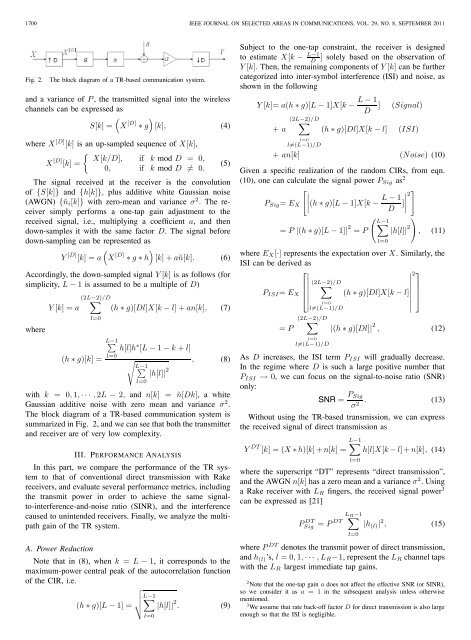
Fig. 2.<br />
The block diagram of a TR-based communication system.<br />
and a variance of P , the transmitted signal into the wireless<br />
channels can be expressed as<br />
( )<br />
S[k] = X [D] ∗ g [k], (4)<br />
where X [D] [k] is an up-sampled sequence of X[k],<br />
{<br />
X [D] X[k/D], if k mod D = 0,<br />
[k] =<br />
(5)<br />
0, if k mod D ≠ 0.<br />
The signal received at the receiver is the convolution<br />
of {S[k]} and {h[k]}, plus additive white Gaussian noise<br />
(AWGN) {ñ i [k]} with zero-mean and variance σ 2 . The receiver<br />
simply performs a one-tap gain adjustment to the<br />
received signal, i.e., multiplying a coefficient a, and then<br />
down-samples it with the same factor D. The signal before<br />
down-sampling can be represented as<br />
(<br />
)<br />
Y [D] [k] =a X [D] ∗ g ∗ h [k]+añ[k]. (6)<br />
Accordingly, the down-sampled signal Y [k] is as follows (for<br />
simplicity, L − 1 is assumed to be a multiple of D)<br />
(2L−2)/D<br />
∑<br />
Y [k] =a (h ∗ g)[Dl]X[k − l]+an[k], (7)<br />
where<br />
l=0<br />
(h ∗ g)[k] =<br />
L−1 ∑<br />
l=0<br />
h[l]h ∗ [L − 1 − k + l]<br />
√<br />
L−1<br />
, (8)<br />
∑<br />
|h[l]| 2<br />
with k = 0, 1, ··· , 2L − 2, and n[k] = ñ[Dk], a white<br />
Gaussian additive noise with zero mean and variance σ 2 .<br />
The block diagram of a TR-based communication system is<br />
summarized in Fig. 2, and we can see that both the transmitter<br />
and receiver are of very low complexity.<br />
III. PERFORMANCE ANALYSIS<br />
In this part, we compare the performance of the TR system<br />
to that of conventional direct transmission with Rake<br />
receivers, and evaluate several performance metrics, including<br />
the transmit power in order to achieve the same signalto-interference-and-noise<br />
ratio (SINR), and the interference<br />
caused to unintended receivers. Finally, we analyze the multipath<br />
gain of the TR system.<br />
A. Power Reduction<br />
Note that in (8), when k = L − 1, it corresponds to the<br />
maximum-power central peak of the autocorrelation function<br />
of the CIR, i.e.<br />
(h ∗ g)[L − 1] = √ L−1 ∑<br />
|h[l]| 2 . (9)<br />
l=0<br />
l=0<br />
Subject to the one-tap constraint, the receiver is designed<br />
to estimate X[k − L−1<br />
D<br />
] solely based on the observation of<br />
Y [k]. Then, the remaining components of Y [k] can be further<br />
categorized into inter-symbol interference (ISI) and noise, as<br />
shown in the following<br />
Y [k]= a(h ∗ g)[L − 1]X[k − L − 1<br />
D ] (Signal)<br />
+ a<br />
(2L−2)/D<br />
∑<br />
l=0<br />
l≠(L−1)/D<br />
(h ∗ g)[Dl]X[k − l] (ISI)<br />
+ an[k] (Noise) (10)<br />
Given a specific realization of the random CIRs, from eqn.<br />
(10), one can calculate the signal power P Sig as 2<br />
[ ∣∣∣∣<br />
P Sig = E X (h ∗ g)[L − 1]X[k − L − 1 ∣ ]<br />
∣∣∣<br />
2<br />
D ]<br />
= P |(h ∗ g)[L − 1]| 2 = P<br />
( L−1<br />
) ∑<br />
|h[l]| 2 , (11)<br />
l=0<br />
where E X [·] represents the expectation over X. Similarly, the<br />
ISI can be derived as<br />
⎡<br />
2⎤<br />
(2L−2)/D<br />
∑<br />
P ISI = E X<br />
⎢<br />
⎣<br />
(h ∗ g)[Dl]X[k − l]<br />
⎥<br />
⎦<br />
l=0<br />
∣<br />
∣<br />
= P<br />
l≠(L−1)/D<br />
(2L−2)/D<br />
∑<br />
l=0<br />
l≠(L−1)/D<br />
|(h ∗ g)[Dl]| 2 , (12)<br />
As D increases, the ISI term P ISI will gradually decrease.<br />
In the regime where D is such a large positive number that<br />
P ISI → 0, we can focus on the signal-to-noise ratio (SNR)<br />
only:<br />
SNR = P Sig<br />
σ 2 . (13)<br />
Without using the TR-based transmission, we can express<br />
the received signal of direct transmission as<br />
L−1<br />
∑<br />
Y DT [k] =(X ∗ h)[k]+n[k] = h[l]X[k − l]+n[k], (14)<br />
where the superscript “DT” represents “direct transmission”,<br />
and the AWGN n[k] has a zero mean and a variance σ 2 .Using<br />
a Rake receiver with L R fingers, the received signal power 3<br />
can be expressed as [21]<br />
P DT<br />
Sig<br />
l=0<br />
L = P ∑ R−1<br />
DT<br />
l=0<br />
|h (l) | 2 , (15)<br />
where P DT denotes the transmit power of direct transmission,<br />
and h (l) ’s, l =0, 1, ··· ,L R −1, representtheL R channel taps<br />
with the L R largest immediate tap gains.<br />
2 Note that the one-tap gain a does not affect the effective SNR (or SINR),<br />
so we consider it as a = 1 in the subsequent analysis unless otherwise<br />
mentioned.<br />
3 We assume that rate back-off factor D for direct transmission is also large<br />
enough so that the ISI is negligible.