0 - Nearfield Systems Inc.

COMPENSATION FOR PROBE TRANSLATION
EFFECTS IN DUAL POLARIZED PLANAR
NEAR-FIELD ANTENNA MEASUREMENTS
Daniël Janse van Rensburg
Nearfield Systems Inc, 19730 Magellan Drive, Torrance, CA 90502, USA.
November 2008 1

Overview
• Planar near-field acquisition
• Probe translation & compensation formulation
• Example 1
• Offset determination
• Example 2
• Conclusions
November 2008 2

Probe Translation Problem
Cable.
y
Pol = 90 degrees.
x
z
x
y
Cable.
Pol = 0 degrees.
November 2008 3

Planar Near-field Scan
November 2008 4

' K P
( P = a F ∫ e
i ⋅
0
S 02 ⋅
'
0
)
PNF Spectral Relations I
'
( ) ( )
iγd
K S10
K e d K
Kerns’ representation of the complex measured voltage on a planar
surface to the AUT plane wave spectral function, where
P = Vector
K = Transverse
b
a
'
0
0
F'
= Mismatch
e
S
'
02
= Complex
= Complex
e
i K • P iγd
relative
= Probe
defining
to
input
= Phase
scan
part
measured
term
near −
of
signal.
signal.
correction term.
relating
probe location.
field
plane centre.
AUT
plane wave spectrum.
probe
location
propagation vector k.
origin
to
Probe spectrum
S
10
=
AUT
plane
wave
spectrum.
November 2008 5

Probe Translation Problem
Cable.
y
Pol = 90 degrees.
x
z
x
y
Cable.
Pol = 0 degrees.
November 2008 6

PNF Spectral Relations II
In order to solve for the complex spectrum of the AUT, two measurement data sets
are required using two near-field probes that have linearly independent spectra,
leading to a set of two equations with two unknowns.
If the equation shown above is regarded as the first data set, the second (after probe
polarization rotation) can be written as
b
'' K P T
P a F e
i ( )
( = ∫
⋅ +
0
S 02 ⋅
''
0
)
''
( ) ( )
iγd
K S10
K e d K
T
b
S
''
0
= Δxxˆ
+ Δyyˆ
''
02
=
Complex
=
Rotated
= Vector defining rotated probe translation.
measured signal for rotated probe.
probe plane wave spectrum.
November 2008 7

Example I: 94 GHz CP Horn
Case #
Δx [mm]
Δx [λ]
Δy[mm]
Δy[λ]
1

Example I: 94 GHz CP Horn
Y (meters)
-0.45
-0.50
-0.55
-0.60
-0.65
0
-2
-4
-6
-8
-10
-12
-14
-16
-18
-20
-22
-24
-26
-28
-30
-32
-34
-36
-38
-40
-42
-44
-46
-48
-50
Y (meters)
-0.45
-0.50
-0.55
-0.60
-0.65
0
-2
-4
-6
-8
-10
-12
-14
-16
-18
-20
-22
-24
-26
-28
-30
-32
-34
-36
-38
-40
-42
-44
-46
-48
-50
-0.70
-0.70
-0.15 -0.10 -0.05 0.00 0.05 0.10
X (meters)
-0.15 -0.10 -0.05 0.00 0.05 0.10
X (meters)
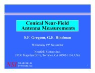
Near-field intensity for CP antenna measured with LP
probe. Δx = 4mm (1.25λ) and Δy = -4.5mm (1.4λ).
Dynamic range shown is 50 dB.
November 2008 9

Example I: 94 GHz CP Horn
0
Uncorrected Corrected Reference
0
Uncorrected Corrected Reference
-5
-5
-10
-10
Amplitude (dB)
-15
-20
-25
Amplitude (dB)
-15
-20
-25
-30
-30
-35
-35
-40
-40 -30 -20 -10 0 10 20 30 40
Elevation (deg)
-40
-40 -30 -20 -10 0 10 20 30 40
Elevation (deg)
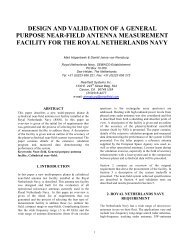
Elevation plane co-polarized (left) and cross-polarized (right)
patterns for 94 GHz CP horn. Case #2 uncorrected data (red),
Case #2 corrected (blue) and Case 1 reference data (purple).
T = 4mm (x) – 4.5mm (y).
November 2008 10

Example I: 94 GHz CP Horn
Far-field amplitude of test_c_11.nsi
Far-field amplitude of test_c_10.nsi
0
0.5 mm 1.5 mm 2.5 mm 3.5 mm 4.5 mm
0
7.5 mm 8.5 mm 9.5 mm 10.5 mm 11.5 mm 12.5 mm
-5
-5
-10
-10
-15
-15
Amplitude (dB)
-20
-25
Amplitude (dB)
-20
-25
-30
-30
-35
-35
-40
-40
-40 -30 -20 -10 0 10 20 30 40 -40 -30 -20 -10 0 10 20 30 40
Elevation (deg)
Elevation (deg)
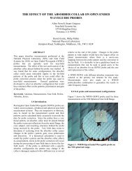
Sensitivity examples for a 1.5λ translation.
Case #2 (left) Case #3 (right).
November 2008 11

Automated Probe Offset Determination
1. Full near-field acquisition with the near-field probe
polarization positions 0° and 90°.
‣ Extract far-field phase data for horizontal (azimuth)
and vertical (elevation) planes.
2. Repeat near-field acquisition with the near-field
probe polarization positions 180° and 270°.
‣ Extract far-field phase data for horizontal (azimuth)
and vertical (elevation) planes.
Cable.
Pol = 90 degrees.
y
3. Subtraction of the two far-field phase reference
patterns is a direct measure of the probe translation
Δx & Δy.
x
x
z
y
Cable.
Pol = 0 degrees.
November 2008 12

Example 2: 23 GHz LP Array
Near-field amplitude of DJvR_Probe_offset01.nsi
0.25
Y (meters)
0.20
0.15
0.10
0.05
0.00
-0.05
-0.10
-0.15
-0.20
0
-2
-4
-6
-8
-10
-12
-14
-16
-18
-20
-22
-24
-26
-28
-30
-32
-34
-36
-38
-40
-42
-44
-46
-48
-50
-0.25
-0.25 -0.20 -0.15 -0.10 -0.05 0.00 0.05 0.10 0.15 0.20 0.25
X (meters)
Near-field intensity for LP slotted waveguide array
measured with LP probe (orthogonal polarization
component is not shown since amplitude < -50 dB ).
Δx = Δy = 3mm (0.23λ at 23.25 GHz). Dynamic
range shown is 50 dB.
November 2008 13

Example 2: 23 GHz LP Array
0
Far-field amplitude of DJvR_Probe_offset01.nsi
0/90 Case 180/270 Case
Far-field phase of DJvR_Probe_offset01.nsi - Far-field phase of DJvR_Probe_offset04.nsi
0/90 Case 180/270 Case Phase difference
-5
150
-10
-15
100
Amplitude (dB)
-20
-25
-30
-35
-40
Phase (deg)
50
0
-50
-100
-45
-50
-50 -40 -30 -20 -10 0 10 20 30 40 50
Azimuth (deg)
-150
-30 -20 -10 0 10 20 30
Azimuth (deg)
Azimuth LP co-polarized anplitude (left) and phase (right) patterns. Probe position
0/90 data (red) and probe position 180/270 (blue). Phase data comparison showing
the 3 mm probe translation effect. The difference between the two phase functions
is also shown and is sinusoidal with respect to the azimuth angle.
November 2008 14

Example 2: 23 GHz LP Array
5.0
Average
The difference between the two phase functions can be
converted to a linear offset Δx using
Probe Offset
Probe x offset
Δx
=
λΔPhase
2π
sinθ
Linear distance [mm]
4.5
4.0
3.5
3.0
2.5
2.0
1.5
1.0
0.5
0.0
-30 -20 -10 0 10 20 30
Azimuth (deg)
Since we know the offset has to be
> 0 and < 5 mm, the average value
of all values in this domain can be
calculated. It follows that:
Δx = (2.98 mm).
Repeating this process for the
elevation plane it follows that:
Δy = (3.04 mm).
November 2008 15

Example 2: 23 GHz LP Array
Far-field phase of NewFilename.nsi
Uncorrected Corrected Reference
Far-field phase of NewFilename.nsi
Uncorrected Corrected Reference
150
150
100
100
50
50
Phase (deg)
0
Phase (deg)
0
-50
-50
-100
-100
-150
-150
-30 -20 -10 0 10 20 30
Azimuth (deg)
-30 -20 -10 0 10 20 30
Elevation (deg)
Far-field azimuth (left) and elevation (right) phase data
comparison demonstrating the T = 2.98mm (x) + 3.04mm (y)
probe translation correction.
November 2008 16

Conclusions
• Technique allows for the correction of planar near-field probe
translation during polarization rotation.
• Significant application in mm-wave applications.
• Self calibration technique has been described that allows for
automated detection of the near-field probe translation distance.
• This technique circumvents the problem of having to make
mechanical measurements of the probe alignment.
November 2008 17