Lecture Notes (PDF) - Aqueous and Environmental Geochemistry

Geochemistry
DM Sherman, University of Bristol
2008/2009
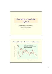
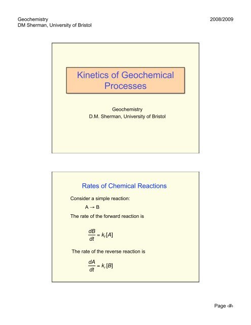
Kinetics of Geochemical
Processes
Geochemistry
D.M. Sherman, University of Bristol
Rates of Chemical Reactions
Consider a simple reaction:
A → B
The rate of the forward reaction is
dB
dt = k f [A]
The rate of the reverse reaction is
!
dA
dt = k r [B]
!
Page ‹#›

Geochemistry
DM Sherman, University of Bristol
2008/2009
Rates of Chemical Reactions
At equilibrium, the rates are equal:
dB
dt = dA
dt
and
k f [A] = k r [B]
!
The equilibrium constant is
K eq = [B]
[A] = k f
k r
!
Reaction Rate Laws In General
In general, for an elementary reaction
aA + bB → cC + dD
the rate of the reaction (neglecting back reaction) is
R = " 1 a
d[A]
dt
= " 1 b
d[B]
dt
= 1 c
d[C]
dt
= 1 d
d[D]
dt
= k f [A] a [B] b
!
where n = a + b is the order of the reaction.
Page ‹#›

Geochemistry
DM Sherman, University of Bristol
2008/2009
Reaction Rate Laws In General
First-order reactions (e.g., A → B):
R = " d[A]
dt
= k f [A]
Second-order reactions (e.g., 2A → B):
!
d[A]
dt
= k f [A] 2
Zeroth-order reactions:
!
d[A]
dt
= k f
!
Integrating Rate laws..
Suppose we have a simple first-order rate law for
the transformation of A:
d[A]
dt
= "k f
[A]
Multiply both sides by dt and rearranging gives..
!
dA = "k f
[A]dt
!
d[A]
[A]
= "k f
dt
!
Page ‹#›

Geochemistry
DM Sherman, University of Bristol
2008/2009
Integrating Rate laws (cont)..
Now we integrate both sides. We have our initial
condition that at t = 0, [A] = [A] 0 .
A d[A] t
" = #kf " dt
[A] 0
A 0
!
"
ln [A] %
$ ' = (k f
t
#[A] 0 &
!
[A] = [A] 0
e "k f t
!
Half-Life
The half-life of A is the time it takes for half of A
to disappear (no reverse reaction):
If
A = A o
e "k f t
!
Then when A = A 0 /2:
t 1/ 2 = 0.693/ k f
!
Page ‹#›

Geochemistry
DM Sherman, University of Bristol
2008/2009
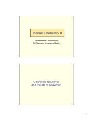
Half-Life
Process
Ion complexation
Adsorption
Gas dissolution
Hydrolysis
Precipitation/Dissolution
Mineral Recrystallization
Half-life

Geochemistry
DM Sherman, University of Bristol
2008/2009
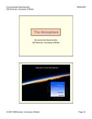
Activation Energies..
Reactions with a high activation energy will show a
strong temperature dependence of their rates. The
measured activation energy can provide mechanistic
clues..
Process !G ‡ (kJ/mol)
Aqueous Diffusion < 20
Ion Adsorption 25
Mineral Dissolution 40-80
Solid State Diffusion 80-480
Transition State Theory: Reaction Rate
and Disequilibrium
Rate net
= Rate forward
" Rate reverse
For an elementary reaction
!
A → B
Rate forward
= k f
[A] = [A] k BT
h e"#G f ± / RT
!
Rate reverse
= k r
[B] = [B] k BT
h e"#G r ± / RT
!
Page ‹#›

Geochemistry
DM Sherman, University of Bristol
2008/2009
Transition State Theory: Reaction Rate
and Disequilibrium
Since ΔG = ΔG ‡ f - ΔG‡ r
Rate forward
Rate reverse
= e"#G f ± / RT
e "#G r ± / RT
/ RT
= e"#G
!
!
Rate net
= Rate forward
(1" e "#G / RT )
Rate net
= Rate forward
(1" Q K )
!
Empirical Rate Laws..
For most reactions, the elementary steps are not known.
Empirical rate laws have been measured, however. For
example the dissolution of gypsum:
CaSO 4 .2H 2 O (gypsum) → Ca 2+ + SO 4
2-
+ 2H 2 O
has the rate law (Langmuir and Melchior, 1985):
d[Ca]
dt
= kA w (C s " C)
With k = 2 x 10 -6 m/s, A w = wet surface area (m 2 )
exposed
!
to a m 3 of water, and C s =15.5 mol/m 3 .
Page ‹#›

Geochemistry
DM Sherman, University of Bristol
2008/2009
Mass-Transfer Limited Reactions
•Reactions for which the elementary chemical steps
are very fast will have rates determined by mass
transfer. Mass transfer can be by diffusion or
advection.
•If diffusion is fast enough, the rate of the reaction will
be advection controlled.
Diffusion: Ficks First Law
The flux (J, in moles/cm 2 -s) of a chemical species is
given by the concentration gradient:
J = "D #C
#x
!
Diffusion constants
of ions in water
range from 10 -6 to
10 -4 cm 2 /s.
Page ‹#›

Geochemistry
DM Sherman, University of Bristol
2008/2009
Diffusion: Ficks Second Law
The concentration as a function of t and x is found
By solving the differential equation (Fick’s 2nd law):
"C
"t
= D " 2 C
"x 2
With the appropriate boundary conditions to define
the problem..
!
Diffusion
For a simple constant-source problem, the boundary
condition is C(0,t) = C 0. The solution to Fick’s 2nd Law is:
C(x,t) = 1 2 C 0(1" erf
x
2 Dt )
!
Page ‹#›

Geochemistry
DM Sherman, University of Bristol
2008/2009
Diffusion
A good approximation for any geometry is that
C(x,t) " 1 4 C 0
when x = Dt
!
Page ‹#›