Assessing Temporary Carbon Storage in Life Cycle Assessment and ...
Assessing Temporary Carbon Storage in Life Cycle Assessment and ...
Assessing Temporary Carbon Storage in Life Cycle Assessment and ...

You also want an ePaper? Increase the reach of your titles
YUMPU automatically turns print PDFs into web optimized ePapers that Google loves.
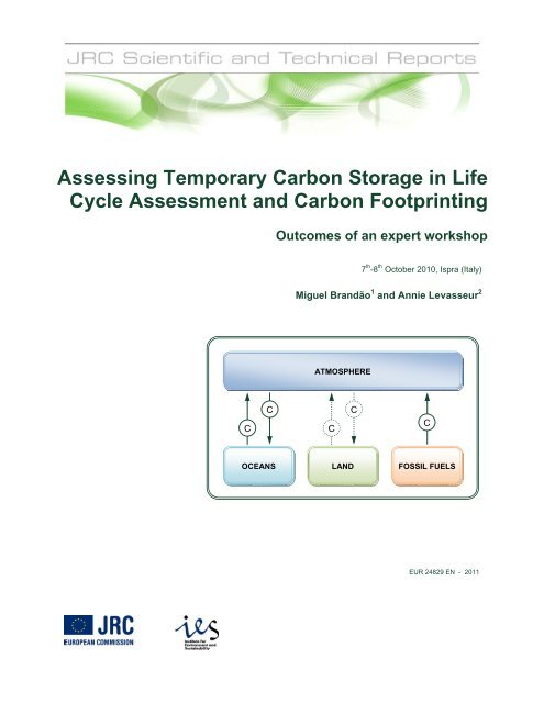
<strong>Assess<strong>in</strong>g</strong> <strong>Temporary</strong> <strong>Carbon</strong> <strong>Storage</strong> <strong>in</strong> <strong>Life</strong><br />
<strong>Cycle</strong> <strong>Assessment</strong> <strong>and</strong> <strong>Carbon</strong> Footpr<strong>in</strong>t<strong>in</strong>g<br />
Outcomes of an expert workshop<br />
7 th -8 th October 2010, Ispra (Italy)<br />
Miguel Br<strong>and</strong>ão 1 <strong>and</strong> Annie Levasseur 2<br />
ATMOSPHERE<br />
C<br />
C<br />
C<br />
C<br />
C<br />
OCEANS LAND FOSSIL FUELS<br />
EUR 24829 EN - 2011
Authors’ affiliation:<br />
1 European Commission, Directorate-General Jo<strong>in</strong>t Research Centre, Institute for Environment<br />
<strong>and</strong> Susta<strong>in</strong>ability, Susta<strong>in</strong>ability <strong>Assessment</strong> Unit, Action 22005 - Environmental <strong>Assessment</strong><br />
<strong>and</strong> the Susta<strong>in</strong>able Use of Resources (ENSURE), European Platform on <strong>Life</strong> <strong>Cycle</strong><br />
<strong>Assessment</strong>, Ispra, Italy<br />
2 CIRAIG – École Polytechnique de Montréal, Chemical Eng<strong>in</strong>eer<strong>in</strong>g Department, Montréal,<br />
Canada<br />
The mission of the JRC-IES is to provide scientific-technical support to the European Union’s policies for the<br />
protection <strong>and</strong> susta<strong>in</strong>able development of the European <strong>and</strong> global environment.<br />
European Commission<br />
Jo<strong>in</strong>t Research Centre<br />
Institute for Environment <strong>and</strong> Susta<strong>in</strong>ability<br />
Contact <strong>in</strong>formation<br />
Jo<strong>in</strong>t Research Centre<br />
Institute for Environment <strong>and</strong> Susta<strong>in</strong>ability<br />
Susta<strong>in</strong>ability <strong>Assessment</strong> Unit<br />
TP 270, I-21027 Ispra (VA), Italy<br />
E-mail: miguel.br<strong>and</strong>ao@jrc.ec.europa.eu<br />
Tel.: +39 0332 785969<br />
Fax: +39 0332 786645<br />
http://ies.jrc.ec.europa.eu/<br />
http://lct.jrc.ec.europa.eu/<br />
Legal Notice<br />
Neither the European Commission nor any person act<strong>in</strong>g on behalf of the Commission is<br />
responsible for the use which might be made of this publication.<br />
Europe Direct is a service to help you f<strong>in</strong>d answers<br />
to your questions about the European Union<br />
Freephone number (*):<br />
00 800 6 7 8 9 10 11<br />
(*) Certa<strong>in</strong> mobile telephone operators do not allow access to 00 800 numbers or these calls may be billed.<br />
A great deal of additional <strong>in</strong>formation on the European Union is available on the Internet.<br />
It can be accessed through the Europa server http://europa.eu/<br />
JRC 63225<br />
EUR 24829 LL<br />
ISBN 978-92-79-20350-3<br />
ISSN 1831-9424<br />
DOI 10.2788/22040<br />
EUR 24829 EN - 2011<br />
Luxembourg: Publications Office of the European Union<br />
© European Union, 2011<br />
Reproduction is authorised provided the source is acknowledged<br />
Pr<strong>in</strong>ted <strong>in</strong> Italy
This report summarises the presentations <strong>and</strong> discussions that took place at the Expert Workshop on<br />
<strong>Temporary</strong> <strong>Carbon</strong> <strong>Storage</strong> for use <strong>in</strong> <strong>Life</strong> <strong>Cycle</strong> <strong>Assessment</strong> (LCA) <strong>and</strong> <strong>Carbon</strong> Footpr<strong>in</strong>t<strong>in</strong>g (CF), held at the<br />
Jo<strong>in</strong>t Research Centre (Ispra, Italy) on 7-8 October 2010. It is presented <strong>in</strong> m<strong>in</strong>utes format with the discussion<br />
grouped <strong>in</strong>to themes rather than reflect<strong>in</strong>g the exact chronological order of the discussion.<br />
Participant’s Name<br />
Fulvio Ardente<br />
Viorel Blujdea<br />
Miguel Br<strong>and</strong>ão<br />
Mirko Busto<br />
Pernilla Cederstr<strong>and</strong><br />
Francesco Cherub<strong>in</strong>i<br />
Kirana Chomkhamsri<br />
Rol<strong>and</strong> Clift<br />
Annette Cowie<br />
Laura Draucker<br />
Fausto Freire<br />
Michele Galatola<br />
Giacomo Grassi<br />
Michael Hauschild<br />
Rol<strong>and</strong> Hiederer<br />
Ari Ilomäki<br />
Susanne Jørgensen<br />
Annemarie Kerkhof<br />
Miko Kirschbaum<br />
Kati Koponen<br />
Annie Levasseur<br />
Gregg Marl<strong>and</strong><br />
Ottar Michelsen<br />
Ivan Munoz<br />
Marta Olejnik<br />
Ana Orive<br />
Rana Pant<br />
Daniele Pernigotti<br />
Glen P. Peters<br />
Pier Porta<br />
Crist<strong>in</strong>a de la Rua<br />
Serenella Sala<br />
Graham S<strong>in</strong>den<br />
Bo Weidema<br />
Mart<strong>in</strong> Weiss<br />
Frank Werner<br />
Marc-Andree Wolf<br />
Kather<strong>in</strong>a Wührl<br />
Giuliana Zanchi<br />
Participant’s Affiliation<br />
EC - DG JRC, Institute for Environment <strong>and</strong> Susta<strong>in</strong>ability, Susta<strong>in</strong>ability <strong>Assessment</strong> Unit, LCA team, Italy<br />
EC - DG JRC, Institute for Environment <strong>and</strong> Susta<strong>in</strong>ability, Climate Change Unit, Italy<br />
SCA Global Hygiene Category, Sweden<br />
Industrial Ecology Programme, Norwegian University of Science <strong>and</strong> Technology (NTNU), Norway<br />
EC - DG JRC, Institute for Environment <strong>and</strong> Susta<strong>in</strong>ability, Susta<strong>in</strong>ability <strong>Assessment</strong> Unit, LCA team, Italy<br />
Centre for Environmental Strategy, University of Surrey, United K<strong>in</strong>gdom<br />
University of New Engl<strong>and</strong>, Australia<br />
World Resources Institute (WRI), USA<br />
Center for Industrial Ecology, University of Coimbra, Portugal<br />
European Commission - DG ENV, EU Ecolabel, Belgium<br />
EC - DG JRC, Institute for Environment <strong>and</strong> Susta<strong>in</strong>ability, Climate Change Unit, Italy<br />
Technical University of Denmark, Section for Quantitative Susta<strong>in</strong>ability <strong>Assessment</strong>, Denmark<br />
EC - DG JRC, Institute for Environment <strong>and</strong> Susta<strong>in</strong>ability, L<strong>and</strong> Management <strong>and</strong> Natural Hazards Unit, Italy<br />
F<strong>in</strong>nish Forest Industries Federation, F<strong>in</strong>l<strong>and</strong><br />
Novozymes, Denmark<br />
PRé Consultants B.V., the Netherl<strong>and</strong>s<br />
L<strong>and</strong>care Research, New Zeal<strong>and</strong><br />
VTT Technical Research Centre of F<strong>in</strong>l<strong>and</strong>, Mitigation of climate change, F<strong>in</strong>l<strong>and</strong><br />
CIRAIG- École Polytechnique de Montréal, Canada<br />
Environmental Sciences Division, Oak Ridge National Laboratory, USA<br />
Industrial Ecology Programme, Norwegian University of Science <strong>and</strong> Technology (NTNU), Norway<br />
Unilever - Safety <strong>and</strong> Environmental Assurance Centre (SEAC), United K<strong>in</strong>gdom<br />
Confederation of European Waste-to-Energy Plants (CEWEP), Belgium<br />
EC - DG JRC, Institute for Environment <strong>and</strong> Susta<strong>in</strong>ability, Climate Change Unit, Italy<br />
EC - DG JRC, Institute for Environment <strong>and</strong> Susta<strong>in</strong>ability, Susta<strong>in</strong>ability <strong>Assessment</strong> Unit, LCA team, Italy<br />
Delegate to the development of the ISO 14067, Italy<br />
Center for International Climate <strong>and</strong> Environmental Research – Oslo (CICERO), Norway<br />
ENEA, Italy<br />
EC - DG JRC, Institute for Environment <strong>and</strong> Susta<strong>in</strong>ability, Susta<strong>in</strong>ability <strong>Assessment</strong> Unit, LCA team, Italy<br />
EC - DG JRC, Institute for Environment <strong>and</strong> Susta<strong>in</strong>ability, Susta<strong>in</strong>ability <strong>Assessment</strong> Unit, LCA team, Italy<br />
The <strong>Carbon</strong> Trust, United K<strong>in</strong>gdom<br />
Eco<strong>in</strong>vent, Switzerl<strong>and</strong><br />
EC - DG JRC, Institute for Environment <strong>and</strong> Susta<strong>in</strong>ability, Transport <strong>and</strong> Air Quality Unit, Italy<br />
Environment & Development, Switzerl<strong>and</strong><br />
EC - DG JRC, Institute for Environment <strong>and</strong> Susta<strong>in</strong>ability, Susta<strong>in</strong>ability <strong>Assessment</strong> Unit, LCA team, Italy<br />
International Organisation for St<strong>and</strong>ardisation (ISO), Switzerl<strong>and</strong><br />
Joanneum Research, Institute of Energy Research, Austria<br />
Acknowledgments:<br />
This report is the result of the consultations with experts, <strong>and</strong> the <strong>in</strong>puts of all of them are acknowledged.<br />
We thank, <strong>in</strong> particular, David Penn<strong>in</strong>gton <strong>and</strong> the experts who presented their papers <strong>in</strong> the workshop:<br />
- Susanne Jørgensen<br />
- Annemarie Kerkhof<br />
- Glen Peters<br />
- Viorel Blujdea<br />
- Marc-Andree Wolf<br />
- Kather<strong>in</strong>a Wührl<br />
- Laura Draucker<br />
- Rol<strong>and</strong> Clift<br />
- Francesco Cherub<strong>in</strong>i<br />
- Giuliana Zanchi<br />
- Annette Cowie<br />
- Annie Levasseur<br />
- Miko Kirschbaum<br />
- Gregg Marl<strong>and</strong>
Executive Summary<br />
L<strong>and</strong> <strong>and</strong> wood products, among others, represent temporary carbon s<strong>in</strong>ks. S<strong>in</strong>ce the<br />
embodied carbon is reta<strong>in</strong>ed outside the atmosphere for a period of time, some radiative<br />
forc<strong>in</strong>g is postponed. <strong>Carbon</strong> removal from the atmosphere <strong>and</strong> storage <strong>in</strong> the biosphere or<br />
anthroposphere, therefore, may have the potential to help mitigate climate change.<br />
<strong>Life</strong> cycle assessment <strong>and</strong> carbon footpr<strong>in</strong>t<strong>in</strong>g are <strong>in</strong>creas<strong>in</strong>gly popular tools for the<br />
environmental assessment of products that take <strong>in</strong>to account their entire life cycle. A robust<br />
method is required to account for the benefits, if any, of temporary carbon storage for use <strong>in</strong><br />
the environmental assessment of products. Despite significant efforts to develop robust<br />
methods to account for temporary carbon storage, there is still no consensus on how to<br />
consider it.<br />
This workshop brought together experts on climate change, carbon footpr<strong>in</strong>t<strong>in</strong>g <strong>and</strong> life cycle<br />
assessment to review available options <strong>and</strong> to discuss the most appropriate method for<br />
account<strong>in</strong>g for the potential benefits of temporary carbon storage. The workshop cont<strong>in</strong>ued<br />
the work developed under the International Reference <strong>Life</strong> <strong>Cycle</strong> Data System (ILCD), which<br />
provides methodological recommendations for use <strong>in</strong> bus<strong>in</strong>ess <strong>and</strong> policy for assess<strong>in</strong>g the<br />
environmental impacts of goods <strong>and</strong> services, tak<strong>in</strong>g <strong>in</strong>to account their full life cycle. This<br />
report is a summary of the presentations <strong>and</strong> discussions held dur<strong>in</strong>g this workshop.
Table of Contents<br />
1 Introduction ...................................................................................................................................... 1<br />
1.1 Background .............................................................................................................................. 1<br />
1.2 Radiative forc<strong>in</strong>g <strong>and</strong> Global Warm<strong>in</strong>g Potentials ................................................................... 2<br />
1.3 Tonne-year approaches ............................................................................................................. 3<br />
1.4 Temporal preferences <strong>and</strong> value choices .................................................................................. 5<br />
1.5 The metrics of climate change .................................................................................................. 6<br />
2 The role of temporary carbon s<strong>in</strong>ks .................................................................................................. 8<br />
2.1 Problems related to temporary carbon storage ......................................................................... 8<br />
2.2 The use of different <strong>in</strong>dicators .................................................................................................. 8<br />
2.3 Benefits of temporary carbon storage ...................................................................................... 9<br />
2.4 Do temporary carbon storage <strong>and</strong> delayed emissions matter? ................................................. 9<br />
3 Exist<strong>in</strong>g approaches <strong>and</strong> rationale for adoption ............................................................................. 11<br />
3.1 LULUCF sector under the Kyoto Protocol ............................................................................ 11<br />
3.2 Exist<strong>in</strong>g approaches for LCA <strong>and</strong> CF .................................................................................... 11<br />
3.3 Develop<strong>in</strong>g approaches for LCA <strong>and</strong> CF ............................................................................... 12<br />
3.4 Account<strong>in</strong>g level ..................................................................................................................... 13<br />
3.5 The choice of a time horizon .................................................................................................. 13<br />
3.6 Discount<strong>in</strong>g future emissions ................................................................................................. 15<br />
3.7 Treatment of biogenic carbon ................................................................................................. 15<br />
3.8 Which approach to choose for carbon footpr<strong>in</strong>t<strong>in</strong>g? .............................................................. 16<br />
4 Application of alternative methods ................................................................................................ 19<br />
5 Conclusions .................................................................................................................................... 21<br />
6 References ...................................................................................................................................... 22<br />
7 Appendix ........................................................................................................................................ 23<br />
7.1 Need for Relevant Timescales <strong>in</strong> <strong>Temporary</strong> <strong>Carbon</strong> <strong>Storage</strong> Credit<strong>in</strong>g ............................... 23<br />
7.2 Treatment of carbon storage <strong>and</strong> delayed emissions .............................................................. 24<br />
7.3 Strengths <strong>and</strong> limitations of the Global Warm<strong>in</strong>g Potential <strong>and</strong> alternative metrics ............. 33<br />
7.4 <strong>Temporary</strong> <strong>Carbon</strong> Sequestration Cannot Prevent Climate Change ...................................... 38<br />
7.5 Account<strong>in</strong>g for sequestered carbon: the value of temporary storage ..................................... 51<br />
7.6 ILCD H<strong>and</strong>book recommendations ........................................................................................ 54<br />
7.7 Treatment of temporary carbon storage <strong>in</strong> PAS 2050 ............................................................ 57<br />
7.8 ISO 14067 <strong>Carbon</strong> footpr<strong>in</strong>t of products ................................................................................ 58<br />
7.9 Greenhouse Gas Protocol Supply Cha<strong>in</strong> Initiative ................................................................. 59<br />
7.10 Biogenic CO2 emissions <strong>and</strong> their contribution to climate change ....................................... 60<br />
7.11 The upfront carbon debt of bioenergy: a comparative assessment ........................................ 61<br />
7.12 Quantify<strong>in</strong>g climate change impacts of bioenergy systems - An overview of the work<br />
of IEA Bioenergy Task 38 on Greenhouse Gas Balances of Biomass <strong>and</strong> Bioenergy Systems ........ 65<br />
7.13 <strong>Assess<strong>in</strong>g</strong> temporary carbon sequestration <strong>and</strong> storage projects through LULUCF<br />
with dynamic LCA ............................................................................................................................. 69
1 Introduction<br />
L<strong>and</strong> <strong>and</strong> wood-based products, among others, represent temporary carbon s<strong>in</strong>ks. S<strong>in</strong>ce the embodied<br />
carbon is reta<strong>in</strong>ed outside the atmosphere for a period of time, some radiative forc<strong>in</strong>g is postponed.<br />
<strong>Carbon</strong> removal from the atmosphere <strong>and</strong> storage <strong>in</strong> the biosphere or anthroposphere, therefore, may<br />
have the potential to help mitigate climate change.<br />
<strong>Life</strong> cycle assessment (LCA) <strong>and</strong> carbon footpr<strong>in</strong>t<strong>in</strong>g (CF) are <strong>in</strong>creas<strong>in</strong>gly popular tools for the<br />
environmental assessment of products that take <strong>in</strong>to account their entire life cycle; from the extraction<br />
of raw materials through to their end-of-life. A robust method is therefore required to account for the<br />
benefits, if any, of temporary carbon storage for use <strong>in</strong> these environmental assessment approaches.<br />
Despite significant efforts, there is still no consensus on how to best consider this.<br />
This workshop brought together experts on climate change, carbon footpr<strong>in</strong>t<strong>in</strong>g <strong>and</strong> life cycle<br />
assessment to review available options <strong>and</strong> to discuss the most appropriate method for account<strong>in</strong>g for<br />
the potential benefits of temporary carbon storage. The workshop cont<strong>in</strong>ued the work developed under<br />
the International Reference <strong>Life</strong> <strong>Cycle</strong> Data System (ILCD) [1], which provides methodological<br />
recommendations for use <strong>in</strong> bus<strong>in</strong>ess <strong>and</strong> policy for assess<strong>in</strong>g the environmental impacts of goods <strong>and</strong><br />
services, tak<strong>in</strong>g <strong>in</strong>to account their full life cycle.<br />
This report is a summary of the presentations <strong>and</strong> discussions held dur<strong>in</strong>g this workshop. Sections 1 to<br />
4 sum up the pr<strong>in</strong>cipal topics of the four sessions of presentations given by experts, <strong>in</strong>clud<strong>in</strong>g<br />
discussions. Section 5 gives the f<strong>in</strong>al conclusions <strong>and</strong> recommendations com<strong>in</strong>g from these<br />
discussions. F<strong>in</strong>ally, the abstracts provided by the different speakers are found <strong>in</strong> the Appendix (see<br />
Section 7).<br />
1.1 Background<br />
There is <strong>in</strong>creas<strong>in</strong>g <strong>in</strong>terest <strong>in</strong> account<strong>in</strong>g for temporary carbon storage <strong>in</strong> the LCA <strong>and</strong> CF of products.<br />
Current LCA methodology does not consider giv<strong>in</strong>g any benefits to temporarily keep<strong>in</strong>g carbon out of<br />
the atmosphere. Indeed, s<strong>in</strong>ce the tim<strong>in</strong>g of emissions is not considered, the amount of carbon<br />
sequestered <strong>in</strong> biomass (negative emission) is simply added to the amount of carbon released at the<br />
product end-of-life (positive emission), which results <strong>in</strong> carbon neutrality. No additional credits are<br />
given for the time of storage.<br />
Some recently published st<strong>and</strong>ards <strong>and</strong> methods, such as the British PAS 2050 [2] <strong>and</strong> the European<br />
Commission’s ILCD H<strong>and</strong>book [1], propose a way to account for the tim<strong>in</strong>g of GHG emissions <strong>in</strong><br />
1
LCA <strong>and</strong> CF. Other st<strong>and</strong>ards <strong>and</strong> methods, still <strong>in</strong> development, such as the WRI/WBCSD GHG<br />
Protocol <strong>and</strong> the ISO 14067, are also look<strong>in</strong>g <strong>in</strong>to this issue. Nevertheless, there is still no consensus<br />
on which method to use, nor on the different value-laden decisions that have to be made, such as the<br />
choice of a time horizon. Section 2 addresses some of these general issues.<br />
1.2 Radiative forc<strong>in</strong>g <strong>and</strong> Global Warm<strong>in</strong>g Potentials<br />
As demonstrated later <strong>in</strong> this report, the time-horizon selected for compar<strong>in</strong>g the impacts of different<br />
greenhouse gases <strong>in</strong> terms of e.g. radiative forc<strong>in</strong>g potential has implications on the relative<br />
importance of temporary carbon storage.<br />
There is generally a consensus <strong>in</strong> LCA <strong>and</strong> CF on the use of Global Warm<strong>in</strong>g Potentials (GWPs),<br />
developed by the International Panel on Climate Change (IPCC), to assess the global warm<strong>in</strong>g impact<br />
of greenhouse gas (GHG) emissions [3]. GWP is a climate-change metric to determ<strong>in</strong>e the relative<br />
contribution of GHG emissions, but it can also be used as a basis to analyse the benefits of carbon<br />
sequestration <strong>and</strong> storage. Time horizons are important <strong>in</strong> deriv<strong>in</strong>g GWPs.<br />
The GWP <strong>in</strong>dex for a given GHG is calculated by divid<strong>in</strong>g the value of the radiative forc<strong>in</strong>g caused by<br />
a unit mass pulse-emission of the gas, <strong>in</strong>tegrated over a given time horizon, by the same value obta<strong>in</strong>ed<br />
for carbon dioxide (CO 2 ) for the same time horizon (see Equation 1).<br />
GWP<br />
x<br />
∫<br />
TH<br />
∫<br />
a<br />
⋅C<br />
0<br />
= TH<br />
aCO2<br />
⋅CCO<br />
0<br />
x<br />
x<br />
( t)<br />
dt<br />
2<br />
( t)<br />
dt<br />
(1)<br />
where a is the <strong>in</strong>stantaneous radiative forc<strong>in</strong>g per unit mass <strong>in</strong>crease <strong>in</strong> the atmosphere [W.m -2 .kg -1 ],<br />
C(t) is the time-dependent atmospheric load follow<strong>in</strong>g a pulse-emission, TH is the time horizon <strong>and</strong> x<br />
st<strong>and</strong>s for the given GHG. For CO 2 , the atmospheric load curve is given by the revised Bern carbon<br />
cycle-climate model [4], <strong>and</strong> for other GHGs, it is given by a first-order decay equation.<br />
The most common time horizon used for GWP is 100 years, s<strong>in</strong>ce it was adopted by the UNFCCC for<br />
the Kyoto Protocol. However, there are other time horizons considered by the IPCC (20 <strong>and</strong> 500<br />
years). The implications of the time horizon are that, essentially, the radiative forc<strong>in</strong>g occurr<strong>in</strong>g after<br />
the adopted time-horizon is not considered, so that more importance is given to the radiative forc<strong>in</strong>g<br />
occurr<strong>in</strong>g with<strong>in</strong> the def<strong>in</strong>ed time-horizon. This has implications on the importance relative to CO 2<br />
given to the different GHGs. It equally has implications <strong>in</strong> relation to the issue of <strong>in</strong>tergenerational<br />
equity, as radiative-forc<strong>in</strong>g impacts after the chosen time-horizon are neglected.<br />
2
One argument for this methodological choice of a 100-year cut-off is the assumption that <strong>in</strong> the future<br />
humanity will be better positioned to cope with climate change through e.g. technological<br />
improvements (see Sections 3.5 <strong>and</strong> 3.6 <strong>and</strong> [5] ).<br />
1.3 Tonne-year approaches<br />
The first presentation, given by the organisers of the workshop, <strong>in</strong>troduced the problematic of<br />
temporary carbon storage, <strong>and</strong> presented the aim of the workshop, which was to review available<br />
options <strong>and</strong> to discuss the most appropriate method for account<strong>in</strong>g for the potential benefits of<br />
temporary carbon storage <strong>in</strong> LCA <strong>and</strong> CF. The Moura-Costa [6] <strong>and</strong> the Lashof [7] methods, both<br />
tonne-year approaches developed for that purpose <strong>and</strong> presented <strong>in</strong> the IPCC special report on l<strong>and</strong><br />
use, l<strong>and</strong>-use change <strong>and</strong> forestry (LULUCF) [8], were presented.<br />
The Moura-Costa <strong>and</strong> the Lashof approaches were proposed ten years ago to account for temporary<br />
carbon storage. Some participants expla<strong>in</strong>ed that these authors were <strong>in</strong>volved <strong>in</strong> the development of<br />
the IPCC special report on LULUCF published <strong>in</strong> 2000 [8], <strong>and</strong> that the subject was closed <strong>in</strong> 2003,<br />
when the IPCC published the good practice guidel<strong>in</strong>es adopt<strong>in</strong>g the mass balance stock change<br />
approach. Some years after that, tim<strong>in</strong>g issues were aga<strong>in</strong> receiv<strong>in</strong>g attention with the development of<br />
the British st<strong>and</strong>ard PAS 2050 for carbon footpr<strong>in</strong>t<strong>in</strong>g, where benefits are given to temporary carbon<br />
storage <strong>and</strong> delayed emissions. Other st<strong>and</strong>ards still <strong>in</strong> development, such as the GHG Protocol <strong>and</strong><br />
ISO14067, are also <strong>in</strong>vestigat<strong>in</strong>g temporal issues.<br />
These tonne-year methods aim at calculat<strong>in</strong>g a credit <strong>in</strong> kg-eq CO 2 for keep<strong>in</strong>g carbon out of the<br />
atmosphere for a given number of years. This credit can then be subtracted from a GHG <strong>in</strong>ventory, as<br />
it is assumed to compensate for the impact of an equivalent GHG emission.<br />
The basel<strong>in</strong>e for these methods is the cumulative radiative forc<strong>in</strong>g, <strong>in</strong>tegrated over a given time<br />
horizon (usually 100 years), caused by a one-tonne pulse-emission of CO 2 . For a time horizon of 100<br />
years, the <strong>in</strong>tegral of the CO 2 decay curve is approximately 48 tonne-years.<br />
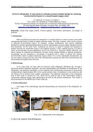
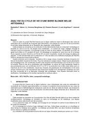
The Moura-Costa approach (see Figure 1) is based on a fixed duration over which impacts occur after<br />
an emission. This reflects typical practice <strong>in</strong> LCA <strong>and</strong> CF, as the time when an emission occurs is not<br />
considered. Accord<strong>in</strong>g to this approach, 48 tonne-years of CO 2 is equivalent to 1 tonne of CO 2 -eq.<br />
Consequently, stor<strong>in</strong>g one tonne of CO 2 for 48 years is equivalent to avoid<strong>in</strong>g the impact of a onetonne<br />
CO 2 emission, which also means that stor<strong>in</strong>g one tonne of CO 2 for one year can fully<br />
compensate for the impact of an emission of 0.02 tonne (1/48) of CO 2 .<br />
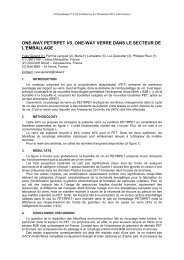
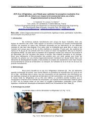
Alternatively, the Lashof approach (see Figure 2) considers that stor<strong>in</strong>g carbon for a given number of<br />
years is equivalent to delay<strong>in</strong>g a CO 2 emission until the end of the storage period. The decay curve is<br />
3
then pushed back from a certa<strong>in</strong> number of years, equal to the storage time, <strong>and</strong> the portion of the<br />
<strong>in</strong>itial 48 tonne-years area which is now beyond the 100-year time horizon corresponds to the benefits<br />
of the perceived storage. For example, when stor<strong>in</strong>g one tonne of CO 2 for a period of 48 years, the<br />
portion of the area under the decay curve beyond 100 years is 19 tonne-years. This means that storage<br />
for 48 years would be equivalent to avoid<strong>in</strong>g an emission of 0.4 tonne (19/48) of CO 2 ; i.e. 40% of the<br />
value of 1 tonne proposed us<strong>in</strong>g the Moura-Costa method for the same sequestration <strong>and</strong> storage<br />
period.<br />
Figure 1. The Moura-Costa approach calculated for a 100-year time horizon. Sequester<strong>in</strong>g <strong>and</strong> stor<strong>in</strong>g<br />
one tonne of CO 2 dur<strong>in</strong>g 48 years (red area) is equivalent to the impact of a 1-tonne CO 2 pulseemission<br />
<strong>in</strong>tegrated over 100 years (blue area).<br />
Figure 2. The Lashof approach calculated for a 100-year time horizon. Sequesterung <strong>and</strong> stor<strong>in</strong>g one<br />
tonne of CO 2 for a period of 48 years is equivalent to delay<strong>in</strong>g a CO 2 emission to t 0 , <strong>and</strong> the benefit is<br />
the portion of the decay curve which is now beyond the 100-year time horizon (blue surface).<br />
4
1.4 Temporal preferences <strong>and</strong> value choices<br />
From Sections 1.2 <strong>and</strong> 1.3, one of the key po<strong>in</strong>ts <strong>in</strong> determ<strong>in</strong><strong>in</strong>g the benefits of temporary carbon<br />
storage is the choice of a time horizon.<br />
From an <strong>in</strong>f<strong>in</strong>ite time perspective, there is no benefit <strong>in</strong> an <strong>in</strong>dividual event considered <strong>in</strong> isolation that<br />
takes carbon out of the atmosphere <strong>and</strong> releases it back later, as the burden is merely shifted further <strong>in</strong><br />
time; unless temporary carbon removals are repeated permanently to ensure an equivalent permanent<br />
carbon removal.<br />
In contrast, adopt<strong>in</strong>g a f<strong>in</strong>ite time perspective implies us<strong>in</strong>g a time horizon beyond which impacts are<br />
not considered. This choice violates the pr<strong>in</strong>ciple of <strong>in</strong>ter-generational equity, embedded <strong>in</strong> the concept<br />
of susta<strong>in</strong>able development, s<strong>in</strong>ce it assumes that e.g. Society will be better able to cope with climate<br />
change <strong>in</strong> the future.<br />
In her presentation (see Section 6.1), Jørgensen raised two conflict<strong>in</strong>g aspects regard<strong>in</strong>g the choice of a<br />
time horizon for the assessment of temporary carbon storage: i) the long-term persistence of CO 2 <strong>in</strong> the<br />
atmosphere, which warrants the consideration of longer time horizons, <strong>and</strong> ii) the urgent risk of<br />
cross<strong>in</strong>g irreversible tipp<strong>in</strong>g po<strong>in</strong>ts, which lead to the use of shorter time horizons to encourage earlier<br />
actions that quickly decrease the atmospheric CO 2 concentration before a tipp<strong>in</strong>g po<strong>in</strong>t is reached.<br />
<strong>Temporary</strong> storage may allow buy<strong>in</strong>g time, but it is important that the chosen time horizon leads to<br />
real climate benefits. To address this contradiction, the authors propose to use two different ways of<br />
credit<strong>in</strong>g climate mitigation, one for the long-term solutions, <strong>and</strong> one for the short-term solutions.<br />
A discussion followed this presentation regard<strong>in</strong>g the relevance of us<strong>in</strong>g two different credit<strong>in</strong>g<br />
systems for both short-term <strong>and</strong> long-term climate mitigation. It is important <strong>in</strong> many assessment<br />
applications, such as for policy options, to clarify the difference between short- <strong>and</strong> long-term actions,<br />
<strong>and</strong> the usefulness/significance of such a dist<strong>in</strong>ction.<br />
As temperature <strong>in</strong>creases, some tipp<strong>in</strong>g po<strong>in</strong>ts may be reached, this is a cont<strong>in</strong>uous process. Jørgensen<br />
expla<strong>in</strong>ed that the idea beh<strong>in</strong>d a short-term credit<strong>in</strong>g system would be to act as a bridg<strong>in</strong>g solution. If it<br />
is assumed that the next 100 or 150 years are critical <strong>and</strong> that tipp<strong>in</strong>g po<strong>in</strong>ts should not be crossed, it<br />
may be beneficial to postpone emissions to a period where the atmospheric concentration will be<br />
lower. Another possibility is to give a higher impact score to short-term emissions than to long-term<br />
emissions on a cont<strong>in</strong>uous scale. A more complete discussion about the time horizon issue can be<br />
found <strong>in</strong> Section 4.5.<br />
In her presentation (see Section 6.2), Kerkhof discussed the general issues regard<strong>in</strong>g the treatment of<br />
temporary carbon storage <strong>and</strong> delayed emissions <strong>in</strong> LCA <strong>and</strong> CF methods:<br />
5
The first issue was the sett<strong>in</strong>g of temporal boundaries <strong>in</strong> LCA. Two different options were presented: i)<br />
to <strong>in</strong>clude all the processes <strong>and</strong> emissions occurr<strong>in</strong>g over the life cycle without any temporal cut-off,<br />
which prevents from giv<strong>in</strong>g any benefit to temporary climate mitigation, or ii) to establish a temporal<br />
boundary <strong>in</strong> the scope of the study.<br />
The second issue was the <strong>in</strong>herent value judgement <strong>in</strong> giv<strong>in</strong>g more importance to present impacts<br />
compared to future ones. Two different worldviews were presented <strong>and</strong> related to the choice of a time<br />
horizon for climate impact assessment: i) valu<strong>in</strong>g sooner emission reduction compared to later ones, <strong>in</strong><br />
opposition to ii) the need to manage carbon now as well as <strong>in</strong> the future without any dist<strong>in</strong>ction.<br />
The third issue looked at how the consideration of temporary carbon storage <strong>and</strong> delayed GHG<br />
emissions can <strong>in</strong>centivise different behaviours, such as choos<strong>in</strong>g durable products or products made<br />
from biogenic materials. A procedure was presented <strong>in</strong> the form of a decision tree to help mak<strong>in</strong>g these<br />
value-laden choices.<br />
1.5 The metrics of climate change<br />
In his presentation (see Section 6.3), Peters expla<strong>in</strong>ed the physical basis of the widely used Global<br />
Warm<strong>in</strong>g Potential (GWP) concept as a metric for climate change, <strong>and</strong> the different value judgements<br />
<strong>in</strong>volved.<br />
Climate change metrics can be based on different <strong>in</strong>dicators, such as radiative forc<strong>in</strong>g, temperature<br />
<strong>in</strong>crease, sea level rise, <strong>and</strong> economic costs; this reflects different levels of modell<strong>in</strong>g along the causeeffect<br />
cha<strong>in</strong> or environmental mechanism. Arguments are hence analogous to those of midpo<strong>in</strong>t vs<br />
endpo<strong>in</strong>t model<strong>in</strong>g discussions that took place <strong>in</strong> the LCA community. They also <strong>in</strong>volve several<br />
choices, such as the use of an <strong>in</strong>stantaneous or an <strong>in</strong>tegrated value, the use of a time horizon,<br />
discount<strong>in</strong>g of future emissions, a constant background or a scenario-based one, account<strong>in</strong>g for<br />
regional variations, etc.<br />
The Global Temperature Potential (GTP) concept was then presented as an alternative metric to GWP,<br />
<strong>and</strong> the differences between both of them were expla<strong>in</strong>ed us<strong>in</strong>g the results of a few case studies.<br />
F<strong>in</strong>ally, the implications of the different value-laden choices <strong>in</strong> the selection of a climate change metric<br />
were discussed.<br />
A question was raised regard<strong>in</strong>g how to apply the use of different metrics to CF, <strong>in</strong> which we want to<br />
have a s<strong>in</strong>gle number to encourage people mak<strong>in</strong>g the right choices. There is probably no answer to<br />
that question, as this presentation showed that we can take different decisions depend<strong>in</strong>g on the metric<br />
6
we are us<strong>in</strong>g, <strong>and</strong> also that these decisions are based on value judgements, such as the choice of a time<br />
horizon, which can vary from one person/group to another.<br />
A discussion followed on how decisions can be made when different metrics are used that give<br />
different answers, <strong>and</strong> different value judgements which can significantly alter the results. It is very<br />
important to know what the target is <strong>and</strong> to identify all the value-laden choices we make explicitly.<br />
Look<strong>in</strong>g at different metrics can help us identify<strong>in</strong>g what we want to promote, <strong>and</strong> then use the metric<br />
that better expresses it. It is also important to make sure that all the choices are consistently made.<br />
7
2 The role of temporary carbon s<strong>in</strong>ks<br />
This session of the workshop presented two oppos<strong>in</strong>g views regard<strong>in</strong>g the role of temporary carbon<br />
storage for climate mitigation.<br />
2.1 Problems related to temporary carbon storage<br />
In his presentation (see Section 6.4), Kirschbaum discussed the effectiveness of us<strong>in</strong>g temporary<br />
carbon storage to mitigate climate change. The widely used GWPs account for the impacts caused by<br />
cumulative temperature <strong>in</strong>creases. Other types of impact on climate change are related to the<br />
<strong>in</strong>stantaneous temperature <strong>in</strong>crease <strong>and</strong> to the rate of temperature <strong>in</strong>crease. He argued that any measure<br />
that <strong>in</strong>cludes only one of these impacts cannot fully capture the full scale of the issue. This<br />
presentation showed, us<strong>in</strong>g climate models <strong>and</strong> different IPCC scenarios for future CO 2 atmospheric<br />
concentrations, that temporary carbon storage only reduces impacts related to the cumulative effect of<br />
<strong>in</strong>creased temperature, <strong>and</strong> can worsen the other types of impact. The message was that the assessment<br />
of the mitigation potential of temporary carbon storage should <strong>in</strong>clude each of these different k<strong>in</strong>ds of<br />
impacts, as well as the feedbacks of the global carbon cycle.<br />
2.2 The use of different <strong>in</strong>dicators<br />
Follow<strong>in</strong>g this presentation, the relation between the three <strong>in</strong>dicators presented (i.e. cumulative<br />
radiative forc<strong>in</strong>g, <strong>in</strong>stantaneous temperature <strong>and</strong> rate of <strong>in</strong>crease <strong>in</strong> temperature) was discussed. The<br />
<strong>in</strong>stantaneous temperature approximately follows the <strong>in</strong>tegrated radiative forc<strong>in</strong>g (plus an impulse<br />
response for temperature), <strong>and</strong> the rate of <strong>in</strong>crease <strong>in</strong> temperature (which is the derivative of the<br />
temperature) is proportional to <strong>in</strong>stantaneous radiative forc<strong>in</strong>g. This means that radiative forc<strong>in</strong>g could<br />
be a good approximate of these three metrics, as long as the <strong>in</strong>stantaneous <strong>and</strong> the cumulative values<br />
are considered to account for the different types of impacts.<br />
The adoption of three different <strong>in</strong>dicators for climate change <strong>in</strong> LCA was proposed to account for the<br />
three different types of impact presented by Kirschbaum, although some participants argued for one<br />
s<strong>in</strong>gle <strong>in</strong>dicator for climate change. This s<strong>in</strong>gle <strong>in</strong>dicator could be developed by go<strong>in</strong>g further <strong>in</strong> the<br />
impact cha<strong>in</strong> (damage model<strong>in</strong>g), while consider<strong>in</strong>g three different pathways (mid-po<strong>in</strong>ts) before<br />
aggregat<strong>in</strong>g, as is done with other impact categories <strong>in</strong> life cycle impact assessment (LCIA). If midpo<strong>in</strong>t<br />
model<strong>in</strong>g is preferred to damage model<strong>in</strong>g, three different <strong>in</strong>dicators would suffice, even though<br />
the general tendency <strong>in</strong> LCA is to have only one <strong>in</strong>dicator. The existence of multiple <strong>in</strong>dicators may<br />
add complexity <strong>in</strong> terms of decision-mak<strong>in</strong>g <strong>and</strong>, hence, may not be well accepted <strong>in</strong> the bus<strong>in</strong>ess <strong>and</strong><br />
policy communities. Nonetheless, only multiple <strong>in</strong>dicators can express both cumulative <strong>and</strong><br />
8
<strong>in</strong>stantaneous impacts. In LCA, some impact categories are covered by multiple <strong>in</strong>dicators at the<br />
midpo<strong>in</strong>t level (e.g. human toxicity uses both cancer <strong>and</strong> non-cancer effects). For <strong>in</strong>clud<strong>in</strong>g<br />
temperature <strong>in</strong>crease <strong>and</strong> rate of change, extensive work is still needed, although it would be promis<strong>in</strong>g<br />
<strong>and</strong> should be <strong>in</strong>vestigated further.<br />
2.3 Benefits of temporary carbon storage<br />
In his presentation (see Section 6.5), Marl<strong>and</strong> gave environmental <strong>and</strong> economic arguments <strong>in</strong> favour<br />
of temporary carbon storage: it buys time for technological progress <strong>and</strong> learn<strong>in</strong>g, it postpones climate<br />
change, some temporary sequestration may become permanent, sequester<strong>in</strong>g carbon keeps us on a<br />
lower carbon path <strong>and</strong> mediates the approach of tipp<strong>in</strong>g po<strong>in</strong>ts, etc. There is also an economic<br />
argument which states that temporary carbon storage has value as long as carbon emissions have a<br />
monetary value, whether this value is related to a cap-<strong>and</strong>-trade system, a carbon tax, or emission<br />
permits. An analogy was developed with the life <strong>in</strong>surance <strong>in</strong>dustry to show that the expected life time<br />
of temporary storage can be described <strong>in</strong> probabilistic terms, <strong>in</strong> order to give it a f<strong>in</strong>ancial value, which<br />
could be used to determ<strong>in</strong>e the cost of the temporary credits. Credits for permanent storage could be<br />
bought <strong>and</strong> sold, <strong>and</strong> credits for temporary storage could be rented.<br />
2.4 Do temporary carbon storage <strong>and</strong> delayed emissions matter?<br />
When assess<strong>in</strong>g temporary carbon storage, a time frame needs to be def<strong>in</strong>ed, s<strong>in</strong>ce there is no benefit<br />
for it on an <strong>in</strong>f<strong>in</strong>ite time basis. If the time frame is 100 years, stor<strong>in</strong>g carbon for a few years is<br />
important, but if the time frame is much longer, it becomes <strong>in</strong>significant. Kirschbaum presented three<br />
types of impact related to global warm<strong>in</strong>g: i) the <strong>in</strong>stantaneous temperature <strong>in</strong>crease, which leads to<br />
extreme weather conditions <strong>and</strong> diseases, ii) the rate of temperature <strong>in</strong>crease, which has an impact on<br />
ecological adaptation, <strong>and</strong> iii) cumulative heat<strong>in</strong>g or radiative forc<strong>in</strong>g, which impacts on long-term<br />
effects such as sea level rise. Stor<strong>in</strong>g carbon for a few years <strong>and</strong> releas<strong>in</strong>g it back to the atmosphere has<br />
two consequences: it decreases the cumulative heat<strong>in</strong>g of the atmosphere over a def<strong>in</strong>ed time frame,<br />
<strong>and</strong> it <strong>in</strong>creases the temperature at a given time <strong>in</strong> the short term. With a longer time horizon, both<br />
effects would become less significant. It is important to determ<strong>in</strong>e whether impacts occurr<strong>in</strong>g <strong>in</strong> the<br />
short-term are more important than those occurr<strong>in</strong>g <strong>in</strong> the long-term.<br />
The carbon cycle is dynamic. Tak<strong>in</strong>g carbon out of the atmosphere has consequences on the carbon<br />
flows elsewhere <strong>in</strong> the cycle, e.g. ocean uptake. Releas<strong>in</strong>g one tonne of carbon to the atmosphere or<br />
stor<strong>in</strong>g it for a period of time <strong>and</strong> releas<strong>in</strong>g it later would lead to different CO 2 concentrations at a<br />
given time <strong>in</strong> the future. It would lead to the same concentration for an <strong>in</strong>f<strong>in</strong>ite time frame, but the<br />
trajectories to that po<strong>in</strong>t there would be different, so the tim<strong>in</strong>g of the emissions matters with f<strong>in</strong>ite<br />
9
time frames. The impact of delay<strong>in</strong>g an emission can be positive for a given metric (cumulative<br />
radiative forc<strong>in</strong>g over a given time frame), <strong>and</strong> negative for another metric (<strong>in</strong>stantaneous temperature<br />
<strong>in</strong>crease at a given time <strong>in</strong> the future).<br />
10
3 Exist<strong>in</strong>g approaches <strong>and</strong> rationale for adoption<br />
The presentations held dur<strong>in</strong>g this session gave an overview of the exist<strong>in</strong>g approaches <strong>and</strong> those<br />
under development.<br />
3.1 LULUCF sector under the Kyoto Protocol<br />
Blujdea presented the way carbon account<strong>in</strong>g is done at the country level for the purposes of meet<strong>in</strong>g<br />
<strong>and</strong> monitor<strong>in</strong>g targets for the Kyoto Protocol, <strong>and</strong> more particularly for the LULUCF (l<strong>and</strong> use, l<strong>and</strong>use<br />
change <strong>and</strong> forestry) sector. Every type of l<strong>and</strong> use must be covered <strong>and</strong> there are different review<br />
processes to check how the numbers are estimated. The account<strong>in</strong>g follows a stock change approach<br />
based on mass balances. Different sources of uncerta<strong>in</strong>ty are related to the account<strong>in</strong>g process. This is<br />
because: assessments are done every 10 years <strong>and</strong> computations are used to get yearly estimates;<br />
emission factors rely on proxies; there is an imbalance between forest, which receives the highest<br />
attention, <strong>and</strong> the other types of l<strong>and</strong> use; there is a lack of transparency for some types of emission;<br />
<strong>and</strong> some carbon flows are not taken <strong>in</strong>to account. <strong>Temporary</strong> carbon storage under clean development<br />
mechanism (CDM) only applies to reforestation <strong>and</strong> aforestation projects. There are two different ways<br />
to account for it: 1) to account for the reduction only when the project is f<strong>in</strong>ished, or 2) to use<br />
temporary certified emission reductions.<br />
Follow<strong>in</strong>g this presentation, it was po<strong>in</strong>ted out that some carbon flows are taken <strong>in</strong>to account at the<br />
country level, but not necessarily <strong>in</strong> the LULUCF sector, which can expla<strong>in</strong> why some carbon flows<br />
seem to be lack<strong>in</strong>g. Flows com<strong>in</strong>g from crops for biofuels, for <strong>in</strong>stance, can be <strong>in</strong>cluded <strong>in</strong> the energy<br />
sector, <strong>and</strong> not <strong>in</strong> the LULUCF one. A dist<strong>in</strong>ction was also made between report<strong>in</strong>g <strong>and</strong> account<strong>in</strong>g.<br />
Changes <strong>in</strong> carbon stocks can be reported, such as the burn<strong>in</strong>g of wood for energy, but are not<br />
necessarily accounted under the Kyoto Protocol target, depend<strong>in</strong>g on the situation.<br />
3.2 Exist<strong>in</strong>g approaches for LCA <strong>and</strong> CF<br />
In his presentation (see Section 6.6), Wolf expla<strong>in</strong>ed how temporary carbon storage <strong>and</strong> delayed GHG<br />
emissions should be taken <strong>in</strong>to account accord<strong>in</strong>g to the ILCD H<strong>and</strong>book [1]. The general rule is that<br />
temporary carbon storage <strong>and</strong> delayed emissions shall not be considered <strong>in</strong> LCA, unless the goal of the<br />
study clearly warrants it. If so, temporarily sequester<strong>in</strong>g <strong>and</strong> stor<strong>in</strong>g carbon <strong>in</strong> a product is argued to be<br />
analogous to delay<strong>in</strong>g a fossil CO 2 emission. The rationale beh<strong>in</strong>d the use of GWP 100 for account<strong>in</strong>g<br />
for the radiative forc<strong>in</strong>g occurr<strong>in</strong>g over the 100 years follow<strong>in</strong>g the assessed emission is its wide<br />
adoption, even though this <strong>in</strong>troduces a time perspective that is not adopted by any other impact<br />
categories.<br />
11
In the <strong>in</strong>ventory, a delayed emission is accounted for with dedicated elementary flows <strong>and</strong> the<br />
emission (<strong>in</strong> kg) is multiplied by the number of years the emission is delayed, up to 100 years. These<br />
flows carry a characterization factor for GWP100 (-0.01, -0.25 <strong>and</strong> -2.98 per kg <strong>and</strong> year for CO 2 , CH 4<br />
<strong>and</strong> N 2 O, respectively). An emission occurr<strong>in</strong>g beyond 100 years shall be <strong>in</strong>ventoried as a long-term<br />
emission.<br />
This approach differentiates biogenic <strong>and</strong> geogenic CO 2 <strong>and</strong> CH 4 elementary flows, <strong>and</strong> allows us<strong>in</strong>g<br />
the same <strong>in</strong>ventory for model<strong>in</strong>g, or not, temporary carbon storage or delayed emissions. Details are<br />
expla<strong>in</strong>ed <strong>in</strong> Appendix 6.6.<br />
The other exist<strong>in</strong>g approach presented (see Section 6.7) by Clift is the British carbon footpr<strong>in</strong>t<strong>in</strong>g<br />
st<strong>and</strong>ard PAS 2050 [2]. The developed method is based on the Lashof approach, which accounts for<br />
carbon storage <strong>in</strong> biomass by look<strong>in</strong>g at the effect of delay<strong>in</strong>g an emission on radiative forc<strong>in</strong>g,<br />
<strong>in</strong>tegrated over a 100-year period. The formulae used <strong>in</strong> PAS 2050 are a l<strong>in</strong>ear approximation of this<br />
concept. There is no discount<strong>in</strong>g applied, but a temporal cut-off is used, s<strong>in</strong>ce any emission occurr<strong>in</strong>g<br />
after 100 years follow<strong>in</strong>g the sale of the product are not considered. The same concept could be<br />
applied to other GHGs, even though this is not done <strong>in</strong> the st<strong>and</strong>ard, as all the GHG emissions are<br />
transformed <strong>in</strong> kg CO 2 -eq before apply<strong>in</strong>g the delay credit.<br />
3.3 Develop<strong>in</strong>g approaches for LCA <strong>and</strong> CF<br />
Two develop<strong>in</strong>g approaches aim<strong>in</strong>g at giv<strong>in</strong>g guidel<strong>in</strong>es for carbon footpr<strong>in</strong>t<strong>in</strong>g of products were also<br />
presented by Wuehrl <strong>and</strong> Draucker. The International St<strong>and</strong>ard Organisation is develop<strong>in</strong>g a new<br />
st<strong>and</strong>ard for carbon footpr<strong>in</strong>t<strong>in</strong>g of products, ISO 14067 (see Section 6.8). This st<strong>and</strong>ard will give<br />
guidel<strong>in</strong>es for the quantification (part 1) <strong>and</strong> communication (part 2) of carbon footpr<strong>in</strong>t of products<br />
<strong>and</strong> services over their life cycle. The f<strong>in</strong>al version is <strong>in</strong>tended to be published at the beg<strong>in</strong>n<strong>in</strong>g of<br />
2012. Several discussions were held <strong>in</strong> the work<strong>in</strong>g group regard<strong>in</strong>g the need to consider temporary<br />
carbon storage, <strong>and</strong> no consensus on the subject is yet to be reached.<br />
The World Resources Institute (WRI) <strong>and</strong> the World Bus<strong>in</strong>ess Council for Susta<strong>in</strong>able Development<br />
(WBCSD) are develop<strong>in</strong>g the Product <strong>Life</strong> <strong>Cycle</strong> Greenhouse Gas Account<strong>in</strong>g St<strong>and</strong>ard (see Section<br />
6.9). The goal of this st<strong>and</strong>ard is to provide guidel<strong>in</strong>es on how to calculate life cycle based GHG<br />
<strong>in</strong>ventories of products or services. Several discussions have been held at different levels of the<br />
organization on the topic of temporary carbon storage <strong>and</strong> delayed emissions, but the f<strong>in</strong>al position is<br />
not yet known, as the st<strong>and</strong>ard is still <strong>in</strong> development like ISO 14067. The position (at the time of the<br />
presentation) is to <strong>in</strong>clude every carbon flow (uptakes <strong>and</strong> emissions), but not to consider their tim<strong>in</strong>g<br />
12
(no credits for storage or delayed emissions), as there is no scientific consensus on the value-laden<br />
choices that need to be made.<br />
3.4 Account<strong>in</strong>g level<br />
Two account<strong>in</strong>g levels were identified: i) the national level, where the focus is on the amount of<br />
carbon stored <strong>in</strong> the forests of a given country or l<strong>and</strong>scape, <strong>and</strong> ii) the project level, where the focus is<br />
on the carbon stored <strong>in</strong> a product throughout its life cycle. The national level type of account<strong>in</strong>g is<br />
used under the Kyoto Protocol; time issues are not considered, as account<strong>in</strong>g relies on mass balances.<br />
A participant mentioned that the product level is <strong>in</strong>adequate, as cutt<strong>in</strong>g trees does not necessarily mean<br />
that carbon is released to the atmosphere if the forest is managed appropriately, because of tree regrowth<br />
<strong>and</strong> carbon accumulation <strong>in</strong> the soil. Others argued that, virtually, the sum of all the project or<br />
product level account<strong>in</strong>gs would give the same result as the national-level account<strong>in</strong>g. The objective of<br />
this workshop is to discuss how we should account for the benefits, if any, of temporarily stor<strong>in</strong>g<br />
carbon <strong>in</strong> a product for LCA <strong>and</strong> carbon footpr<strong>in</strong>t<strong>in</strong>g purposes, so that the product level will be used<br />
for the follow<strong>in</strong>g discussions.<br />
3.5 The choice of a time horizon<br />
A discussion followed regard<strong>in</strong>g the choice of a time horizon. A participant criticized the use of a 100-<br />
year cut-off, say<strong>in</strong>g that it would encourage people to emit GHGs at year 99, so that their impact<br />
would be considered only over one year. The use of a 100-year time horizon would also encourage<br />
fossil emissions to become acceptable, as long as some temporary carbon storage compensates for it.<br />
Another participant mentioned that the idea beh<strong>in</strong>d the use of GWP100 is to provide a relative<br />
weight<strong>in</strong>g of the different GHGs, <strong>and</strong> that the choice of a time horizon is merely to fix this ratio, but<br />
that does not mean that impacts occurr<strong>in</strong>g after that time horizon are neglected (which is the rationale<br />
beh<strong>in</strong>d those approaches). It was po<strong>in</strong>ted out that the aim of PAS 2050, for <strong>in</strong>stance, is to look at the<br />
impacts on global warm<strong>in</strong>g of a given purchase, so it is logical to br<strong>in</strong>g all the life cycle emissions on a<br />
common time scale. A too short time horizon would give more weight to delayed releases, <strong>and</strong> we may<br />
not want to promote that. On the other h<strong>and</strong>, a too long time horizon would not take <strong>in</strong>to account that<br />
someth<strong>in</strong>g must be done about climate forc<strong>in</strong>g emissions with<strong>in</strong> the next few years, <strong>and</strong> not with<strong>in</strong> the<br />
next centuries.<br />
The choice of a time horizon is an important aspect <strong>in</strong> assess<strong>in</strong>g temporary carbon storage. A time<br />
horizon of 100 years is generally chosen because it is used for policies, such as those related to the<br />
Kyoto Protocol. The question was raised whether a 100-year time frame should be used for every<br />
13
impact category <strong>in</strong> LCA, for consistency reasons. Some participants argued that the time horizon<br />
matters only for a few impact categories, <strong>and</strong> that it should not be applied to all of them.<br />
An extract from a paper written by Keith Sh<strong>in</strong>e, one of the lead authors who proposed the GWP<br />
concept <strong>in</strong> the IPCC First <strong>Assessment</strong> Report, was read: “It seems to be widely believed that the Kyoto<br />
Protocol chose a 100-year time horizon because it was the middle one of the three: 20, 100 <strong>and</strong> 500<br />
years that happened to be presented <strong>in</strong> the IPCC report. There is certa<strong>in</strong>ly no conclusive scientific<br />
argument that can defend 100 years compared to any other choices, <strong>and</strong> <strong>in</strong> the end the choice is a<br />
value-laden one. And no matter how uncomfortable the concept of discount<strong>in</strong>g can be to physical<br />
scientists, the choice of any time horizon short of <strong>in</strong>f<strong>in</strong>ity is, de facto, a decision to impose some k<strong>in</strong>d<br />
of discount<strong>in</strong>g.” [5] Any limited time frame is arbitrary. In LCIA, most methods are us<strong>in</strong>g the<br />
GWP100 for def<strong>in</strong><strong>in</strong>g characterization factors for climate change, but not all of them. IMPACT2002+<br />
is us<strong>in</strong>g 500 years because it is closer to <strong>in</strong>f<strong>in</strong>ity. But us<strong>in</strong>g an <strong>in</strong>f<strong>in</strong>ite time frame for global warm<strong>in</strong>g<br />
would result <strong>in</strong> CO 2 hav<strong>in</strong>g an impact, <strong>and</strong> other GHGs would be negligible, as the CO 2 concentration<br />
follow<strong>in</strong>g a pulse-emission never returns to pre-emission levels.<br />
A question was raised as to whether the three <strong>in</strong>dicators presented by Kirschbaum would have<br />
different time perspectives. The relevant time horizon can be different for each of them, depend<strong>in</strong>g on<br />
the emergency of the problem. Sea level rise, represented by cumulative radiative forc<strong>in</strong>g, may not be<br />
a problem <strong>in</strong> the short term, but will be <strong>in</strong> 300 or 400 years. For this reason, a 500-year time frame<br />
could be preferable <strong>in</strong>stead of 100 years. The <strong>in</strong>stantaneous temperature <strong>in</strong>crease <strong>and</strong> the rate of<br />
change are more related to short-term impacts. A tipp<strong>in</strong>g po<strong>in</strong>t may be reached for temperature <strong>in</strong> a<br />
near future beyond which any mitigation action would be irrelevant. For these two metrics, us<strong>in</strong>g a<br />
shorter time horizon may be more relevant, as it is more urgent to reduce these impacts. The choice of<br />
a time horizon has a decisive <strong>in</strong>fluence on the value given to temporary carbon storage.<br />
The time horizon already used <strong>in</strong> LCIA for GWP represents the time over which the impact is<br />
<strong>in</strong>tegrated after the emission occurs, <strong>and</strong> has noth<strong>in</strong>g to do with the life cycle <strong>in</strong>ventory time frame.<br />
For long life cycles, there is an <strong>in</strong>consistency between this time horizon, used to assess climate change<br />
impacts, <strong>and</strong> the time frame chosen for the analysis. If a given time horizon is chosen because it is<br />
assumed that problems occurr<strong>in</strong>g dur<strong>in</strong>g this time period are more important, relative to the po<strong>in</strong>t <strong>in</strong><br />
time where we are now, the impacts should be assessed on a period go<strong>in</strong>g from when the emission<br />
occurs until the end of this time frame, calculated from the present time. With actual LCA, it is<br />
considered that all the emissions are occurr<strong>in</strong>g now, but as soon as it matters to account for the<br />
moment when these emissions occur, it is not consistent to use a fixed time horizon for GWP.<br />
14
A fixed time horizon can be used (e.g. 100 years), which beg<strong>in</strong>s at the moment the first emission<br />
occurs, or a variable time horizon, which also beg<strong>in</strong>s at the moment when the first emission occurs, but<br />
f<strong>in</strong>ishes on a given year (e.g. 2100). With a fixed time horizon, the impact is assessed over the 100<br />
years follow<strong>in</strong>g the first emission. With a variable time horizon, the impact is assessed over a time<br />
horizon beg<strong>in</strong>n<strong>in</strong>g when the first emission occurs <strong>and</strong> f<strong>in</strong>ish<strong>in</strong>g <strong>in</strong> e.g. 2100. Policies are usually<br />
look<strong>in</strong>g at a given po<strong>in</strong>t <strong>in</strong> time on which some targets are fixed. The same can be done <strong>in</strong> LCA <strong>and</strong> a<br />
variable time horizon can be used. However, the problem with a variable time horizon is that it will<br />
change through time. Each decade, for example, it will probably be pushed back another 10 years, so<br />
that it will be constantly updated. PAS 2050 <strong>and</strong> the ILCD H<strong>and</strong>book 1 use a fixed time horizon as they<br />
are look<strong>in</strong>g at the radiative forc<strong>in</strong>g occurr<strong>in</strong>g 100 years follow<strong>in</strong>g the formation of the product. To be<br />
consistent, an assessment done next year should use the same characterization factors as an assessment<br />
done today, which means that it is better to use a fixed time horizon.<br />
3.6 Discount<strong>in</strong>g future emissions<br />
A dist<strong>in</strong>ction was made between the choice of a time horizon <strong>and</strong> discount<strong>in</strong>g, two different ways to<br />
express time preferences. Choos<strong>in</strong>g a time horizon consists <strong>in</strong> look<strong>in</strong>g at a particular environmental<br />
problem, which can be measured <strong>and</strong> documented, <strong>and</strong> then <strong>in</strong> mak<strong>in</strong>g decisions on the emergency of<br />
the situation or the relevance of future actions. Discount<strong>in</strong>g is based on the assumption that future<br />
impacts are less important because future generations will be better able to cope with the damage.<br />
There is science beh<strong>in</strong>d discount<strong>in</strong>g (economics, social science), but it is different from the “physical<br />
discount<strong>in</strong>g” on which time horizons are based. The general attitude <strong>in</strong> the LCIA community is to<br />
avoid discount<strong>in</strong>g <strong>and</strong> time cut-offs. The choice of time horizons or discount rates is value-laden, but<br />
cannot be excluded from this subject because it is impossible to give a value to temporary carbon<br />
storage without us<strong>in</strong>g time preferences.<br />
3.7 Treatment of biogenic carbon<br />
A general discussion followed on the treatment of biogenic carbon uptakes <strong>and</strong> emissions. The first<br />
comment was about the tim<strong>in</strong>g of the sequestration. If you have a forest, you cut a tree at time zero to<br />
make a wooden product, <strong>and</strong> then you plant another tree that will grow thereafter, the sequestration is<br />
not occurr<strong>in</strong>g at time zero, but is also delayed. This temporal issue should also be considered <strong>in</strong> the<br />
calculations.<br />
The other issue treated was whether credits should be given to temporary carbon storage only <strong>and</strong> only<br />
if a new s<strong>in</strong>k is created. Some argued that credits should not be given to transfer carbon from one non-<br />
1 This is the case provided that temporary carbon storage or delayed emissions are part of the goal of the LCA.<br />
15
atmospheric s<strong>in</strong>k to another (from a tree to a wooden product, from crude oil to a plastic product, etc.),<br />
<strong>and</strong> that credits should only be given for tak<strong>in</strong>g carbon out of the atmosphere <strong>in</strong> an additional s<strong>in</strong>k.<br />
Follow<strong>in</strong>g this rationale, the only products that would get the credits are those com<strong>in</strong>g from a new<br />
aforestation project, dist<strong>in</strong>guish<strong>in</strong>g forests established with the <strong>in</strong>tention of sequester<strong>in</strong>g carbon from<br />
st<strong>and</strong>ard managed forests. But here, a mechanism would be needed to make sure that the protected<br />
recent forest would not come at the expense of an unprotected old forest. Others argued that delay<strong>in</strong>g a<br />
fossil emission is equivalent to stor<strong>in</strong>g carbon <strong>in</strong> biomass, the only difference between both be<strong>in</strong>g the<br />
sequestration for the case of biogenic carbon storage. S<strong>in</strong>ce the atmosphere does not make the<br />
difference between fossil <strong>and</strong> biogenic carbon, delayed fossil or biogenic emissions should be treated<br />
on the same basis. The difference is that, <strong>in</strong> the case of the biomass, there is a negative emission to<br />
consider for the carbon uptake from the atmosphere. To be consistent, we need to look at the flows of<br />
carbon between the product <strong>and</strong> the atmosphere. And if the decision to account for the tim<strong>in</strong>g of these<br />
flows is taken, it has to be done for every emission, regardless of their orig<strong>in</strong>.<br />
3.8 Which approach to choose for carbon footpr<strong>in</strong>t<strong>in</strong>g?<br />
The pr<strong>in</strong>cipal conclusion from the previous discussions was that it may be needed to look at other<br />
<strong>in</strong>dicators than GWP for climate change impact assessment. As these developments need time <strong>and</strong><br />
resources for research, <strong>and</strong> as there is actually an important <strong>in</strong>ternational consensus on the use of<br />
GWP100, the follow<strong>in</strong>g discussion aimed at giv<strong>in</strong>g recommendations on how to assess temporary<br />
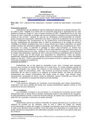
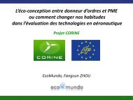
carbon storage <strong>and</strong> delayed emissions us<strong>in</strong>g the GWP concept <strong>and</strong> a given time horizon. Four options<br />
were discussed to determ<strong>in</strong>e how the tim<strong>in</strong>g of the emissions should be accounted for <strong>in</strong> CF us<strong>in</strong>g the<br />
cumulative radiative concept (see Figure 3). The x-axis represents the time when the emission is<br />
occurr<strong>in</strong>g, <strong>and</strong> the y-axis is the relative impact of this emission.<br />
16
Relative impact of an emission occurr<strong>in</strong>g at year t<br />
1<br />
0<br />
Option 1: Fixed GWP<br />
Option 2: Moura‐Costa<br />
Option 3a: ILCD<br />
Option 3b: PAS2050<br />
Option 4: Dynamic AGWP<br />
0 50 100<br />
Time (years)<br />
Figure 3. Illustration of the four options discussed for the assessment of temporary carbon storage <strong>and</strong><br />
delayed emissions <strong>in</strong> LCA <strong>and</strong> CF<br />
A time horizon (100 years <strong>in</strong> Figure 3) is chosen beyond which the impact is zero, because the<br />
problem is considered no longer relevant. Option 1 reflects a constant characterization factor. The<br />
problem with this option is that a high value is given for an emission occurr<strong>in</strong>g one year before the<br />
time horizon, <strong>and</strong> then no value for an emission occurr<strong>in</strong>g one year after. That means that a substantial<br />
benefit would be given for delay<strong>in</strong>g an emission one year more, which does not reflect reality. For<br />
long time horizons, the consequences of this would not be significant, but for shorter time horizons, it<br />
is better to use a decreas<strong>in</strong>g characterization factor. Option 2 is the Moura-Costa approach. The<br />
problem with this option, as stated <strong>in</strong> Section 2.1, is that it is <strong>in</strong>consistent with the concept of time<br />
horizon, s<strong>in</strong>ce the benefit of delay<strong>in</strong>g a unit mass pulse-emission from a number of years equal to the<br />
time horizon is higher than the total impact of this emission <strong>in</strong>tegrated over this time horizon. That is<br />
why the impact of a delayed emission reaches zero at 48 years <strong>in</strong>stead of 100 years. Option 3, as used<br />
<strong>in</strong> the ILCD H<strong>and</strong>book <strong>and</strong> the PAS 2050 st<strong>and</strong>ard, is a l<strong>in</strong>ear approximation of option 4, which is<br />
dynamic AGWP, or the Lashof approach. A l<strong>in</strong>ear approximation has the advantage of be<strong>in</strong>g very<br />
simple to use <strong>in</strong> LCA, as the yearly benefit for delay<strong>in</strong>g an emission is constant. As the difference<br />
17
etween the l<strong>in</strong>ear approximation (option 3) <strong>and</strong> the full approach (option 4) is not very significant, it<br />
could be used <strong>in</strong> LCA <strong>and</strong> CF.<br />
18
4 Application of alternative methods<br />
The way biogenic carbon uptakes <strong>and</strong> emissions are treated <strong>in</strong> different studies have been presented <strong>in</strong><br />
this session of the workshop. In his presentation (see Section 6.10), Francesco Cherub<strong>in</strong>i <strong>in</strong>troduced a<br />
new <strong>in</strong>dicator, GWP bio , which was developed to assess the climate change impact of biogenic CO 2<br />
emissions while consider<strong>in</strong>g the dynamics of vegetation re-growth. Biogenic CO 2 emissions are<br />
actually considered neutral, s<strong>in</strong>ce the released carbon will be sequestered aga<strong>in</strong> by the biomass.<br />
However, these emissions cause an impact on radiative forc<strong>in</strong>g before they are captured by vegetation<br />
re-growth. The GWP bio <strong>in</strong>dex is expressed as a function of the rotation period of the biomass, <strong>and</strong> can<br />
be applied to any type of biomass species. It relies on the impulse response function orig<strong>in</strong>ated from<br />
the perturbation caused by a CO 2 emission to the atmosphere, as expressed by the Bern carbon cycleclimate<br />
model. The consequences of us<strong>in</strong>g this new <strong>in</strong>dicator at a product level <strong>and</strong> at a national<br />
account<strong>in</strong>g level were presented.<br />
Zanchi (see Section 6.11) <strong>in</strong>troduced the concept of the carbon neutrality factor (CN) to quantify the<br />
GHG emission reduction caused by the use of biomass as an energy source. This factor is def<strong>in</strong>ed as<br />
the ratio between the net reduction/<strong>in</strong>crease of carbon emissions <strong>in</strong> the bioenergy system <strong>and</strong> the<br />
carbon emissions from the substituted reference system, over a certa<strong>in</strong> period of time. Currently, GHG<br />
emissions com<strong>in</strong>g from the combustion of biomass are assumed neutral. When the time needed to<br />
sequester back this carbon <strong>in</strong> re-grow<strong>in</strong>g biomass is long, the capability of bioenergy to reduce the<br />
GHG emissions on a short- to medium-term is reduced. The discussion on bioenergy carbon neutrality<br />
is important, s<strong>in</strong>ce the European Union adopted ambitious policy targets on the use of renewable<br />
energy sources. The CN for different bioenergy case studies were quantified <strong>and</strong> discussed.<br />
Bioenergy was also the subject of the follow<strong>in</strong>g presentation given by Annette Cowie (see Section<br />
6.12), which raised different issues regard<strong>in</strong>g the assessment of GHG mitigation benefits of bioenergy<br />
projects as identified by the IEA Bioenergy Task 38. Bioenergy systems are not carbon neutral, as<br />
several GHG emissions arise from other life cycle stages (biomass production, fuel production,<br />
transportation, etc.). The expansion of bioenergy can also lead to <strong>in</strong>direct l<strong>and</strong> use change (LUC)<br />
emissions, s<strong>in</strong>ce biomass production for energy may displace food production. To account for the<br />
tim<strong>in</strong>g of emissions <strong>and</strong> removals, the concept of Net Present Value (NPV) of radiative forc<strong>in</strong>g over<br />
100 years has been developed under Task 38. Bioenergy systems that <strong>in</strong>volve l<strong>and</strong> use change can also<br />
<strong>in</strong>fluence climate through impacts on albedo, which can be quantified <strong>and</strong> added to the calculation.<br />
The st<strong>and</strong>ard methodology for the assessment of bioenergy systems was presented, <strong>and</strong> some case<br />
studies discussed, with a particular focus on biochar.<br />
19
F<strong>in</strong>ally, the dynamic LCA approach (see Section 6.13), developed to account for the tim<strong>in</strong>g of the<br />
emissions <strong>in</strong> LCA, was presented by Levasseur, as well as its application to a case study assess<strong>in</strong>g the<br />
ability of an afforestation project to mitigate an <strong>in</strong>itial fossil-fuel based CO 2 pulse-emission. The<br />
dynamic LCA approach considers the temporal distribution of GHG emissions over the life cycle, <strong>and</strong><br />
calculates their impact on radiative forc<strong>in</strong>g at any time us<strong>in</strong>g dynamic characterization factors, which<br />
consist of the absolute global warm<strong>in</strong>g potential <strong>in</strong>tegrated cont<strong>in</strong>uously through time. The dynamic<br />
LCA approach enables to determ<strong>in</strong>e consistently the time-dependent impact on radiative forc<strong>in</strong>g for<br />
every GHG <strong>and</strong> for any type of product or project life cycle. It also allows decision-makers to test the<br />
sensitivity of the results to the choice of different time horizons.<br />
20
5 Conclusions<br />
This report summarises the ma<strong>in</strong> methodological issues regard<strong>in</strong>g the benefits of temporary carbon<br />
storage <strong>and</strong> associated metrics that were identified <strong>in</strong> the presentations <strong>and</strong> subsequently discussed<br />
throughout the workshop.<br />
Climate benefits of an isolated temporary carbon storage event arise solely when time preferences are<br />
reflected <strong>in</strong> the method used. This means that account<strong>in</strong>g for any benefits relies on value-laden<br />
methodological decisions, such as the choice of a time horizon beyond which impacts are not<br />
considered. Indeed, the longer the time horizon adopted for <strong>in</strong>tegration of radiative forc<strong>in</strong>g or impacts,<br />
the lower the benefits are from temporary carbon storage. This will only be different if the temporary<br />
storage is repeated, essentially becom<strong>in</strong>g a permanent removal from the atmosphere.<br />
If temporary storage is considered then it is common practice to adopt a 100-year time horizon us<strong>in</strong>g<br />
the Global Warm<strong>in</strong>g Potential <strong>in</strong>dex. <strong>Temporary</strong> storage benefits are then generally based on the<br />
Moura-Costa <strong>and</strong> Lashof approaches; assum<strong>in</strong>g that (sequestration <strong>and</strong>) storage of 1 tonne for 48 <strong>and</strong><br />
100 years is essentially equivalent to not emitt<strong>in</strong>g 1 tonne.<br />
However, no clear consensus has been reached from these discussions regard<strong>in</strong>g whether or not to<br />
account for temporary carbon storage <strong>in</strong> general <strong>and</strong>, if so, which method to employ. The choice of a<br />
100-year time horizon equally rema<strong>in</strong>s controversial<br />
S<strong>in</strong>ce the benefits given to temporary carbon storage rely on value-laden choices, if considered then it<br />
is important to make them explicit <strong>and</strong> transparent when us<strong>in</strong>g any account<strong>in</strong>g method. Both short <strong>and</strong><br />
long term time horizons should be considered.<br />
It was suggested to do more research <strong>in</strong> order to improve climate-change modell<strong>in</strong>g <strong>in</strong> LCA to <strong>in</strong>clude<br />
two other <strong>in</strong>dicators (i.e. <strong>in</strong>stantaneous temperature <strong>in</strong>crease <strong>and</strong> rate of temperature <strong>in</strong>crease), s<strong>in</strong>ce<br />
they provide <strong>in</strong>formation on different types of climate-change impact, <strong>and</strong> can lead to different<br />
conclusions than the s<strong>in</strong>gle use of cumulative radiative forc<strong>in</strong>g. Furthermore, research is warranted on<br />
the dynamics of the carbon cycle (e.g. changes <strong>in</strong> s<strong>in</strong>ks – biospheric, atmospheric <strong>and</strong> oceanic – are<br />
<strong>in</strong>terdependent <strong>and</strong> cannot be assessed <strong>in</strong> the same l<strong>in</strong>ear way as fossil emissions with GWP). This is<br />
because any change <strong>in</strong> biospheric carbon stocks may be partially or totally compensated by the <strong>in</strong>verse<br />
process from other s<strong>in</strong>ks (e.g. oceans), so this dynamism needs to be addressed.<br />
21
6 References<br />
[1] European Commission – Jo<strong>in</strong>t Research Centre – Institute for Environment <strong>and</strong> Susta<strong>in</strong>ability.<br />
(2010). International Reference <strong>Life</strong> <strong>Cycle</strong> Data System (ILCD) H<strong>and</strong>book - General guide for<br />
<strong>Life</strong> <strong>Cycle</strong> <strong>Assessment</strong> - Detailed Guidance. Luxembourg: Publications Office of the European<br />
Union.<br />
[2] British St<strong>and</strong>ards Institute <strong>and</strong> the <strong>Carbon</strong> Trust (2008). PAS 2050:2008 Specification for the<br />
assessment of the life cycle greenhouse gas emissions of goods <strong>and</strong> services. London: British<br />
St<strong>and</strong>ards Institute.<br />
[3] Forster, P., Ramaswamy, V., Artaxo, P., Berntsen, T., Betts, R., Fahey, D. W., et al. (2007).<br />
Changes <strong>in</strong> Atmospheric Constituents <strong>and</strong> <strong>in</strong> Radiative Forc<strong>in</strong>g. In S. Solomon, D. Qu<strong>in</strong>, M.<br />
Mann<strong>in</strong>g, Z. Chen, M. Marquis, K.B. Averyt, et al. (eds.), Climate Change 2007: The Physical<br />
Science Basic. Contribution of Work<strong>in</strong>g Group I to the Fourth <strong>Assessment</strong> Report of the<br />
Intergovernmental Panel on Climate Change (pp. 129-234). Cambridge: Cambridge University<br />
Press.<br />
[4] Joos, F., Prentice, I. C., Sitch, S., Meyer, R., Hooss, G., Plattner, G.-K., et al. (2001) Global<br />
warm<strong>in</strong>g feedbacks on terrestrial carbon uptake under the Intergovernmental Panel on Climate<br />
Change (IPCC) emission scenarios. Global Biogeochemical <strong>Cycle</strong>s, 15(4), 891-907.<br />
[5] Sh<strong>in</strong>e, K. P. (2009) The global warm<strong>in</strong>g potential - the need of an <strong>in</strong>terdiscipl<strong>in</strong>ary retrial.<br />
Climatic Change, 96, 467-472.<br />
[6] Moura-Costa, P., & Wilson, C. (2000) An equivalence factor between CO 2 avoided emissions<br />
<strong>and</strong> sequestration - description <strong>and</strong> applications <strong>in</strong> forestry. Mitigation <strong>and</strong> Adaptation<br />
Strategies for Global Change, 5, 51-60.<br />
[7] Fearnside, P. M., Lashof, D. A., & Moura-Costa, P. (2000) Account<strong>in</strong>g for time <strong>in</strong> mitigat<strong>in</strong>g<br />
global warm<strong>in</strong>g through l<strong>and</strong>-use change <strong>and</strong> forestry. Mitigation <strong>and</strong> Adaptation Strategies for<br />
Glogal Change, 5, 239-270.<br />
[8] International Panel on Climate Change (2000) L<strong>and</strong> Use, L<strong>and</strong>-Use Change <strong>and</strong> Forestry.<br />
Cambridge: Cambridge University Press.<br />
22
7 Appendix<br />
7.1 Need for Relevant Timescales <strong>in</strong> <strong>Temporary</strong> <strong>Carbon</strong> <strong>Storage</strong> Credit<strong>in</strong>g<br />
Susanne Vedel Jørgensen <strong>and</strong> Michael Hauschild<br />
When evaluat<strong>in</strong>g possible global warm<strong>in</strong>g mitigation potential of temporary carbon storage, it should<br />
be recognized that the challenge is two-fold: One aspect is the long-term persistence of anthropogenic<br />
CO 2 <strong>in</strong> the atmosphere, another is the urgent risk of cross<strong>in</strong>g possibly irreversible tipp<strong>in</strong>g po<strong>in</strong>ts. For<br />
the long-term issue, only storage of carbon on timescales long enough to simultaneously remove<br />
carbon from the near-surface parts of the global carbon cycle is relevant <strong>in</strong> terms of mitigation<br />
potential. This contradicts many current suggestions for credit<strong>in</strong>g of temporary carbon storage, only<br />
consider<strong>in</strong>g removal from the atmosphere by natural uptake <strong>in</strong> terrestrial biosphere <strong>and</strong> upper ocean.<br />
From these superficial s<strong>in</strong>ks, the carbon has a great risk of re-emission, due to e.g. global warm<strong>in</strong>g.<br />
Closer exam<strong>in</strong>ation of the global carbon cycle reveals timescales of thous<strong>and</strong>s of years for removal of<br />
carbon from the near-surface parts, whereas regeneration of fossil fuels takes millions of years. Many<br />
current suggestions for credit<strong>in</strong>g temporary carbon storage, however, are based on a 100-year time<br />
horizon for global warm<strong>in</strong>g potential, which seems <strong>in</strong>sufficient compared to the removal times of the<br />
global carbon cycle. It is illustrated how this time horizon disregards the long atmospheric lifetime of<br />
anthropogenic CO 2 , hid<strong>in</strong>g long-term impacts of fossil fuel consumption <strong>and</strong> how the decision on time<br />
horizon is essential for the credit<strong>in</strong>g results, mak<strong>in</strong>g it crucial that the chosen time horizon ensures real<br />
climatic benefits. For the urgency issue however, storage on much shorter timescales may have a<br />
‘bridg<strong>in</strong>g potential’ <strong>in</strong> terms of buy<strong>in</strong>g time. For this aspect, timescales need only be long enough to<br />
reach <strong>in</strong>to a more carbon neutral future. It is recommended to separate credit<strong>in</strong>g of global warm<strong>in</strong>g<br />
mitigation potential for the long-term issue <strong>and</strong> the short-term bridg<strong>in</strong>g potential, so possible shortterm<br />
solutions can be acknowledged without appear<strong>in</strong>g to solve long-term problems.<br />
23
7.2 Treatment of carbon storage <strong>and</strong> delayed emissions<br />
Annemarie Kerkhof <strong>and</strong> Mark Goedkoop<br />
7.2.1. Introduction<br />
At the CAIRO TC207 meet<strong>in</strong>g, the draft carbon footpr<strong>in</strong>t st<strong>and</strong>ard was discussed. One of the issues<br />
discussed was whether the st<strong>and</strong>ard should have specific rules to account for carbon storage <strong>and</strong><br />
delayed emission, such as is described <strong>in</strong> PAS 2050. The discussion focussed on the complexity of the<br />
topic; however, this is not just a technical discussion as the treatment of storage <strong>and</strong> delay emissions<br />
means mak<strong>in</strong>g value choices.<br />
The core discussion centres on the treatment of future (delayed) emissions <strong>and</strong> their impact, which can<br />
be grouped <strong>in</strong>to two broad approaches:<br />
1. by treat<strong>in</strong>g all emissions from a product, no matter when they occur, as hav<strong>in</strong>g been<br />
produced when the product was produced, or<br />
2. by treat<strong>in</strong>g future (delayed) emissions from a product differently to those emissions<br />
occurr<strong>in</strong>g today.<br />
With this paper we address three aspects of the debate: the LCA perspective; the value choice<br />
perspective; <strong>and</strong> the “<strong>in</strong>centivis<strong>in</strong>g behaviour” perspective.<br />
7.2.2. The LCA perspective<br />
When conduct<strong>in</strong>g a LCA under ISO 14040/44, establish<strong>in</strong>g a system boundary is an essential part of<br />
conduct<strong>in</strong>g the study. The system boundary establishes cut-offs, result<strong>in</strong>g <strong>in</strong> some processes (<strong>and</strong> their<br />
emissions) not be<strong>in</strong>g considered <strong>in</strong> the study. For carbon footpr<strong>in</strong>t<strong>in</strong>g, the time boundary for the<br />
release of emissions (<strong>and</strong> their subsequent impact) needs to be considered: the impact of specify<strong>in</strong>g a<br />
time boundary or not is discussed below.<br />
7.2.2.1. No time boundary<br />
The LCA <strong>in</strong>cludes all emissions aris<strong>in</strong>g at any future time from the life cycle of the product (<strong>and</strong> their<br />
subsequent impact) as part of the study. This ensures that the footpr<strong>in</strong>t of the product fully reflects the<br />
total GHG impact of the product over time; however, this approach has some adverse consequences:<br />
24
• It would not be possible to ga<strong>in</strong> a benefit from semi-permanent storage, such as thorough<br />
forestry projects or carbon capture <strong>and</strong> storage, as the carbon conta<strong>in</strong>ed <strong>in</strong> these processes will<br />
be released at some po<strong>in</strong>t <strong>in</strong> the future <strong>and</strong> would therefore <strong>in</strong>cluded <strong>in</strong> the LCA of the product;<br />
• It would ignore the real benefit aris<strong>in</strong>g from carbon storage <strong>in</strong> products. (E.g. timber build<strong>in</strong>g<br />
materials store carbon, <strong>and</strong> results <strong>in</strong> less atmospheric carbon.)<br />
• It would result <strong>in</strong> differences <strong>in</strong> product life cycles be<strong>in</strong>g ignored (for two products with<br />
different emissions profiles, this approach would treat the products as be<strong>in</strong>g identical).<br />
• It could encourage short-lived products, as there would be no <strong>in</strong>centive to manufacture longerlived<br />
products that store carbon out of the atmosphere.<br />
7.2.2.2. Time boundary<br />
Consistent with exist<strong>in</strong>g LCA <strong>and</strong> carbon footpr<strong>in</strong>t<strong>in</strong>g st<strong>and</strong>ards, a time boundary is established as part<br />
of the scope of the study that follows one of the two approaches described below:<br />
a) Time boundary on the GWP impact of emissions from the supply cha<strong>in</strong> (PAS 2050<br />
approach), where the damage aris<strong>in</strong>g from emissions released as part of the supply<br />
cha<strong>in</strong> of the product is established 1 ; or<br />
b) Time boundary on emissions from the supply cha<strong>in</strong>, <strong>in</strong>clud<strong>in</strong>g emissions occurr<strong>in</strong>g<br />
with<strong>in</strong> the time boundary of the study together with the full GWP impact of those<br />
emissions.<br />
Under these approaches:<br />
• Products are assessed on a consistent time basis, ensur<strong>in</strong>g that the impact of emissions<br />
occurr<strong>in</strong>g with<strong>in</strong> the boundary of the study are treated on a consistent basis;<br />
• The benefit of longer-last<strong>in</strong>g products that store carbon is reflected <strong>in</strong> this approach; <strong>and</strong><br />
• (For b above) The full GWP impact of emissions occurr<strong>in</strong>g with<strong>in</strong> the time boundary are<br />
<strong>in</strong>cluded (i.e. if emissions occur with<strong>in</strong> the time boundary then the full GWP impact of the<br />
emissions is <strong>in</strong>cluded, even though this extends beyond the 100 year time boundary)<br />
7.2.2.3. Guidance from the LCA st<strong>and</strong>ards perspective<br />
The ISO 14040/44 st<strong>and</strong>ard establishes the need for boundaries; however, it is not very clear on<br />
whether <strong>and</strong> how time boundaries are to be used (note that the st<strong>and</strong>ard is clear that the system<br />
25
oundary for data collection is not related to the boundaries for the impact assessment). Under ISO<br />
14044, a m<strong>and</strong>atory aspect of life cycle impact assessment is “the temporal aspects, such as duration,<br />
residence time, persistence, tim<strong>in</strong>g, etc.” of the category <strong>in</strong>dicator or characterization model.<br />
The current draft of the European LCA h<strong>and</strong>book does have a rule for carbon storage (us<strong>in</strong>g a similar<br />
approach to PAS2050, although simpler – See Annex), <strong>and</strong> suggests report<strong>in</strong>g carbon storage as a<br />
separate parameter 2 : it does not address delayed emissions. Other publications address<strong>in</strong>g the temporal<br />
boundary issue <strong>in</strong>clude the Environmental Eng<strong>in</strong>eers’ H<strong>and</strong>book <strong>and</strong> the H<strong>and</strong>book on life cycle<br />
assessment (operational guide to the ISO st<strong>and</strong>ards).<br />
7.2.3. The value judgement perspective<br />
Both the storage <strong>and</strong> the delayed emission express the assumption that future impacts are less serious<br />
than present impacts. There are a number of perspectives on this choice.<br />
7.2.3.1.Worldview 1: we value emission reduction sooner rather than later<br />
One worldview is to consider we have an urgent climate crisis to solve now, <strong>and</strong> thus we should value<br />
mechanisms that reduce emissions over the shorter term (or shift present emissions to the future). This<br />
view is already implicit <strong>in</strong> many national <strong>and</strong> global policy processes: the IPCC publishes GWP data<br />
on 20, 100 <strong>and</strong> 500 year bases, yet the 100 year timeframe is almost universally used as the basis for<br />
GHG assessment. This has important implications, as the use of 20 year <strong>and</strong> 500 year GWP data would<br />
encourage different actions (e.g. if 20 year GWP data was used, action aga<strong>in</strong>st methane emissions<br />
would be much more important; if 500 year GWP data was used, it would encourage greater action on<br />
SF6 emissions).<br />
The worldview 1 is basically an optimistic view, with regards to what future generations can manage.<br />
The view can be partially justified when we look what has happened <strong>in</strong> previous environmental issues,<br />
like the ozone layer depletion. This was very urgent <strong>in</strong> the n<strong>in</strong>eties; now there is general agreement<br />
that ozone deplet<strong>in</strong>g emissions after 2040 will hardly have an impact. It is of course not clear if this is<br />
also true for carbon. However, it could also reflect concern that unless climate change is successfully<br />
addressed <strong>in</strong> the short term, the world will reach tipp<strong>in</strong>g po<strong>in</strong>ts that no amount of future reduction will<br />
address.<br />
26
7.2.3.2. Worldview 2: we need to manage carbon now <strong>and</strong> <strong>in</strong> the future<br />
Under this worldview, climate change rema<strong>in</strong>s a very urgent issue dur<strong>in</strong>g a much longer term, <strong>and</strong> that<br />
future generations face a similar, or even more serious problems, try<strong>in</strong>g to manage carbon emissions.<br />
Future emissions may <strong>in</strong> this respect be even more serious, as a result of improv<strong>in</strong>g knowledge on<br />
climate science <strong>and</strong> as a result of historic emissions, <strong>and</strong> future generations have little ability to<br />
<strong>in</strong>fluence delayed emissions, as these emissions will be determ<strong>in</strong>ed by decisions taken now.<br />
This world view is not optimistic about the options for manag<strong>in</strong>g carbon at a later stage. This view can<br />
be supported, if we see the very big differences <strong>in</strong> economic development <strong>in</strong> comb<strong>in</strong>ation with the still<br />
very large fossil reserves <strong>in</strong> tar s<strong>and</strong>s <strong>and</strong> coal. It may be very difficult to resist the temptation to use<br />
these resources to generate wealth for people. In that respect the ozone layer problem solution was<br />
much easier, as cheap alternatives were available.<br />
7.2.4. The “<strong>in</strong>centivis<strong>in</strong>g behaviour” perspective<br />
All decisions taken <strong>in</strong> ISO 14067 will <strong>in</strong>centivise different types of behaviour: decisions around which<br />
gases to <strong>in</strong>clude will <strong>in</strong>centivise action around different gases, while decisions about the treatment of<br />
l<strong>and</strong> use change emissions will <strong>in</strong>centivise different approaches to l<strong>and</strong> management.<br />
The approach to carbon storage will similarly <strong>in</strong>centivise different behaviour, <strong>and</strong> <strong>in</strong> this respect it is<br />
important to consider which behaviour we want the st<strong>and</strong>ard to <strong>in</strong>centivise. Products that store<br />
biogenic carbon, or delay emissions release to some time <strong>in</strong> the future, provide a real benefit <strong>in</strong> terms<br />
of reduc<strong>in</strong>g emissions now (compared to equivalent products that do not store or delay emissions).<br />
Should ISO 14067 create the <strong>in</strong>centive for organisation to take these actions? Or should the st<strong>and</strong>ard<br />
be neutral towards the time aspect, <strong>and</strong> both <strong>in</strong>centivis<strong>in</strong>g the reduction on the long <strong>and</strong> the short term.<br />
In essences this question is different depend<strong>in</strong>g on the worldview taken.<br />
Establish<strong>in</strong>g a time boundary will benefit products that store or delay emissions. It will be favourable<br />
to durable products, unfavourable for products with a short lifetime, <strong>and</strong> will benefit biogenic<br />
materials. It also implies we value short term over long-term emission reduction, as future generations<br />
have to live with the choices we make now. It is also consistent with established LCA practice of<br />
def<strong>in</strong><strong>in</strong>g study boundaries.<br />
Includ<strong>in</strong>g all emissions recognises that future emissions arise (to a large degree) from decisions made<br />
today; however, it is <strong>in</strong>consistent with concepts of sequestration <strong>and</strong> storage, <strong>and</strong> does not represent<br />
the benefit of atmospheric carbon be<strong>in</strong>g reta<strong>in</strong>ed <strong>in</strong> storage <strong>in</strong> products for the near future.<br />
27
It is very difficult to make such a value judgement; however, a decision to set a time boundary or not<br />
will be a value judgement. One basis for such a value judgement is to refer to <strong>in</strong>ternationally accepted<br />
policy organisation views, <strong>and</strong> some examples are:<br />
• Brundtl<strong>and</strong> Report: Susta<strong>in</strong>able development is development that meets the needs of the<br />
present without compromis<strong>in</strong>g the ability of future generations to meet their own needs. “Not<br />
compromis<strong>in</strong>g future generation” would, <strong>in</strong> a strict sense, mean a time boundary is not<br />
supported. The Brundtl<strong>and</strong> def<strong>in</strong>ition is accepted by the United Nations as the concept for<br />
susta<strong>in</strong>ability. IPCC is a part of UNEP, but IPCC seems to focus most of its assessments on the<br />
period cover<strong>in</strong>g about one hundred years. In the TAR2007 report the long-term problems are<br />
however often mentioned.<br />
• Although not an <strong>in</strong>ternational body, but widely recognised as pr<strong>in</strong>ciple, the Stern review,<br />
http://en.wikipedia.org/wiki/Stern_Review clearly demonstrates that the cost effectiveness of<br />
carbon management on a short term is very high compared to carbon management on a long<br />
term.<br />
7.2.5. Proposed procedure for mak<strong>in</strong>g the choice<br />
In order to make the choice between a st<strong>and</strong>ard that accounts for carbon storage <strong>and</strong> delayed<br />
emissions, version a st<strong>and</strong>ard that does not support this, the follow<strong>in</strong>g decision tree could be used. The<br />
procedure starts with the value choice, as this is the most important reference. Next there are choices to<br />
be made on whether only storage or also delayed emissions are to be rewarded, <strong>and</strong> whether the reward<br />
of delayed or stored carbon are an optional <strong>and</strong> separate th<strong>in</strong>g to report.<br />
28
7.2.6. Annex 1: Approach <strong>in</strong> PAS 2050<br />
PAS 2050 adopts a time boundary on the impact of emissions approach when assess<strong>in</strong>g the carbon<br />
footpr<strong>in</strong>t of products. This annex provides further details of the approach used <strong>in</strong> PAS 2050, <strong>and</strong> also<br />
provides a discussion of the difference between discount<strong>in</strong>g <strong>and</strong> boundary-sett<strong>in</strong>g.<br />
7.2.6.1. <strong>Carbon</strong> storage <strong>and</strong> delayed emissions <strong>in</strong> PAS 2050<br />
In PAS 2050, two rules are used to take <strong>in</strong>to account the carbon storage <strong>and</strong> the delayed emissions.<br />
These rules reflect the time boundary established by PAS 2050, as this st<strong>and</strong>ard assesses the impact of<br />
GHG emissions aris<strong>in</strong>g from the product over the 100 years follow<strong>in</strong>g formation of the product.<br />
7.2.6.1.1. <strong>Carbon</strong> storage<br />
Biogenic carbon (carbon stored <strong>in</strong> plants) that is released when the plant material is burned, is not<br />
<strong>in</strong>cluded <strong>in</strong> the product carbon footpr<strong>in</strong>t. 3 In addition, where carbon of biogenic orig<strong>in</strong> is stored <strong>in</strong> a<br />
product for more than one year (but released with<strong>in</strong> 100 years) a weight<strong>in</strong>g factor is used to reflect the<br />
proportion of emissions impact occurr<strong>in</strong>g with<strong>in</strong> the 100 year assessment period. The formula used is:<br />
t o = number of years between formation of the product <strong>and</strong> the s<strong>in</strong>gle release of the emissions<br />
29
The stored amount of carbon is multiplied with this weight<strong>in</strong>g factor to calculate the benefit of storage.<br />
Relevant examples are carbon stored <strong>in</strong> wooden build<strong>in</strong>g materials, paper used for books, or long<br />
recycl<strong>in</strong>g cha<strong>in</strong>s, etc. (under PAS 2050, carbon benefit cannot be claimed for food or feed).<br />
7.2.6.1.2. Delayed emissions<br />
The release of fossil carbon is counted as an emission; however, where emissions take place more than<br />
one year follow<strong>in</strong>g formation of the product, the proportion of emissions occurr<strong>in</strong>g with<strong>in</strong> the time<br />
boundary of the study is determ<strong>in</strong>ed. The formula is:<br />
i = each year <strong>in</strong> which emissions occur<br />
x = the proportion of total emissions occurr<strong>in</strong>g <strong>in</strong> an year i<br />
Relevant examples are: A car that emits carbon dur<strong>in</strong>g 10 years, or a low energy light bulb over 20<br />
years.<br />
7.2.6.2. Term<strong>in</strong>ology: discount<strong>in</strong>g <strong>and</strong> boundaries<br />
The establishment of time boundaries <strong>in</strong> LCA studies for the treatment of GHG emissions is<br />
sometimes referred to as discount<strong>in</strong>g: this is not correct. The follow<strong>in</strong>g po<strong>in</strong>ts summarise the<br />
difference between these two approaches to emissions assessment.<br />
7.2.6.2.1. Discount<strong>in</strong>g<br />
Economists often assume that future costs will be lower than present costs, <strong>and</strong> so apply a discount<br />
rate. There is often discussion regard<strong>in</strong>g what the discount rate is, <strong>and</strong> discount rates are often partially<br />
based on <strong>in</strong>terest rates, <strong>in</strong>flation <strong>and</strong> the perception of stakeholders: a discount rate of 3% means that<br />
costs that occur 100 years from now are hardly visible. While be<strong>in</strong>g accepted <strong>in</strong> economic theory, it is<br />
not necessarily accepted <strong>in</strong> environmental issues: for example, there is little evidence of people<br />
discount<strong>in</strong>g their concerns regard<strong>in</strong>g nuclear waste, even though the problem may occur <strong>in</strong> the distant<br />
future.<br />
Under a discount<strong>in</strong>g approach, future emissions are assumed to have less impact than emissions<br />
produced now: this view could be justified by assum<strong>in</strong>g that climate change is less of a problem <strong>in</strong> the<br />
future, or that the cost of mitigation is lower <strong>in</strong> the future. Importantly, all emissions are <strong>in</strong>cluded <strong>in</strong> a<br />
discount<strong>in</strong>g approach (i.e. there is no time boundary); it is the significance of these emissions<br />
compared to current-day emissions that is “discounted”.<br />
30
7.2.6.2.2.Boundary sett<strong>in</strong>g<br />
By establish<strong>in</strong>g a time boundary for the LCA study (e.g. 100 years follow<strong>in</strong>g formation of the<br />
product), emissions or the impact of emissions occurr<strong>in</strong>g with<strong>in</strong> the time boundary can proceed. This<br />
approach does not discount future emissions, but rather it identifies which emissions are with<strong>in</strong> the<br />
boundaries of the study, <strong>and</strong> which are not. This is consistent with the exist<strong>in</strong>g LCA st<strong>and</strong>ards (ISO<br />
14040/44) which require the boundary to the study to be specified; <strong>in</strong> some cases emissions may fall<br />
outside the boundary of the study, but this is not considered with<strong>in</strong> LCA methods to be “discount<strong>in</strong>g”.<br />
7.2.6.3. Consistency with IPCC timeframes<br />
In the PAS2050 are reference is made to the fact that the IPCC equivalency factors are used with a<br />
timeframe of 100 year, <strong>and</strong> that therefore the emissions <strong>in</strong>ventory also need to have a time frame of<br />
100 years. This is not so much an ethical perspective but more a consistency argument. IPCC never<br />
<strong>in</strong>tended to express the fact that emissions tak<strong>in</strong>g place <strong>in</strong> the future are less important, but it<br />
<strong>in</strong>troduced three different time perspectives for compar<strong>in</strong>g the relative impact of different greenhouse<br />
gases. Most people use the 100 years perspective, but IPCC also publishes relative factors for a 20 <strong>and</strong><br />
a 500 year perspective. The impact of CO 2 itself is not changed under these assumptions, only the<br />
impact of substances with an environmental lifetime that is either shorter or longer than the CO 2<br />
lifetime (approx 150 years) does change. Scientifically there is no reason to prefer one over the other;<br />
the choice is based on the same considerations discussed <strong>in</strong> this paper.<br />
7.2.7.Annex 2: The ISO st<strong>and</strong>ards on time boundary<br />
The 14040/44 st<strong>and</strong>ards do not explicitly require or even def<strong>in</strong>e the concept of time boundary. They<br />
usually refer to the concept of system boundary, which is def<strong>in</strong>ed as:<br />
system boundary: set of criteria specify<strong>in</strong>g which unit processes are part of a product system<br />
NOTE The term “system boundary” is not used <strong>in</strong> this International St<strong>and</strong>ard <strong>in</strong> relation to LCIA.<br />
The only reference regard<strong>in</strong>g the temporal aspects <strong>in</strong> LCIA is <strong>in</strong> ISO14044:<br />
4.4.2.2.3: Depend<strong>in</strong>g on the environmental mechanism <strong>and</strong> the goal <strong>and</strong> scope, spatial <strong>and</strong> temporal<br />
differentiation of the characterization model relat<strong>in</strong>g the LCI results to the category <strong>in</strong>dicator should<br />
be considered. The fate <strong>and</strong> transport of the substances should be part of the characterization model.<br />
This means that the temporal aspects should be taken <strong>in</strong>to account <strong>in</strong> the LCIA phase, but it does not<br />
refer to a l<strong>in</strong>k with LCIA. The note on the def<strong>in</strong>ition of the term system boundary seems to <strong>in</strong>dicate<br />
that there is no l<strong>in</strong>k between the temporal boundary <strong>in</strong> LCI <strong>and</strong> the temporal characteristics <strong>in</strong> the<br />
impact assessment.<br />
31
7.2.8. Annex 3: Methodology proposed <strong>in</strong> the Draft European h<strong>and</strong>book on LCA<br />
Extract from the draft European H<strong>and</strong>book on LCA<br />
12.10.4 <strong>Temporary</strong> removal of carbon dioxide from the atmosphere <strong>in</strong> long-liv<strong>in</strong>g products, l<strong>and</strong>fills,<br />
storages<br />
(Refers to aspects of ISO 14044 chapters 4.2.3.5, 4.2.3.6.2 <strong>and</strong> 4.3.2.1)<br />
Consultation note: The 100 years time perspective allows to separately address emissions that act<br />
beyond that time. The use of 100 year (compared to e.g. 20 or 500 years) is a choice that relates not<br />
only but also <strong>and</strong> very prom<strong>in</strong>ently to temporary carbon storage. Feedback on the general issue is<br />
specifically welcomed.<br />
The temporary removal of carbon dioxide from the atmosphere by <strong>in</strong>corporation <strong>in</strong>to long-liv<strong>in</strong>g biobased<br />
products, <strong>in</strong>to bio-based material rema<strong>in</strong>s <strong>in</strong> l<strong>and</strong>fills, or <strong>in</strong> CO 2 -underground-storages is<br />
accounted for, as follows: the duration for which LCIA impacts of released emissions is calculated, is<br />
typically explicitly or implicitly <strong>in</strong>def<strong>in</strong>ite. Exclusively <strong>in</strong> case of the Global Warm<strong>in</strong>g Potential<br />
(GWP) the much shorter perspective “GWP 100 years” is widely used (details <strong>and</strong> recommendations<br />
are provided <strong>in</strong> the separate LCIA guidance documents of the ILCD H<strong>and</strong>book). The related<br />
characterisation factors used are typically those provided as part of the Intergovernmental Panel on<br />
Climate Change (IPCC) reports. Climate change is hence implicitly considered to be a problem of the<br />
next 100 years (3 to 4 generations). The long-term removal of CO 2 from the atmosphere <strong>and</strong> storage <strong>in</strong><br />
long-liv<strong>in</strong>g goods is hence politically promoted.<br />
The difficulty is that the GWP 100 relates to the effect after the emission has taken place i.e. it counts<br />
the climate change impact of emissions that occur nowadays exert with<strong>in</strong> the next 100 years. However,<br />
these emissions may also occur <strong>in</strong> the future (<strong>in</strong> e.g. 80 years when a now newly built house is broken<br />
down). Assign<strong>in</strong>g a full GWP 100 factor to these emissions that happen <strong>in</strong> 80 years would contradict<br />
the logic of the GWP 100 detailed above, as <strong>in</strong> that case their climate change effect for 180 years from<br />
now would be accounted for. Also, no <strong>in</strong>centive would exist to temporarily store the CO 2 e.g. <strong>in</strong> the<br />
wooden beams of the house <strong>in</strong> the above example.<br />
1 Establish<strong>in</strong>g a time boundary is not the same as discount<strong>in</strong>g emissions; see the annex for further discussion.<br />
2 The GHG equivalent stored is multiplied by the number of years stored; the result is presented as kg CO 2 .yr.<br />
3 Biogenic materials are not necessary carbon neutral, as GHG emissions from processes such as grow<strong>in</strong>g, harvest<strong>in</strong>g <strong>and</strong><br />
transport<strong>in</strong>g biogenic materials, <strong>and</strong> from l<strong>and</strong>-use changes, are still <strong>in</strong>cluded under the PAS 2050 approach.<br />
32
7.3 Strengths <strong>and</strong> limitations of the Global Warm<strong>in</strong>g Potential <strong>and</strong><br />
alternative metrics<br />
Glen P. Peters <strong>and</strong> J.S. Fuglestvedt<br />
The United Nations Framework Convention on Climate Change (UNFCCC) requires climate policies<br />
to ‘be cost-effective so as to ensure global benefits at the lowest possible cost’ <strong>and</strong> that ‘policies <strong>and</strong><br />
measures should ... be comprehensive … [<strong>and</strong>] … cover all relevant sources, s<strong>in</strong>ks <strong>and</strong> reservoirs’.<br />
Many studies have shown the advantages of a comprehensive multi-gas agreement, but challenges<br />
rema<strong>in</strong> <strong>in</strong> how to compare the climatic effect of different greenhouse gases (GHGs) [1]. The Kyoto<br />
Protocol (KP) sets limits on the emissions of six long-lived GHGs that are weighted together us<strong>in</strong>g the<br />
Global Warm<strong>in</strong>g Potential with a time-horizon of 100 years (GWP 100 ).<br />
Despite the policy acceptance of the GWP 100 via the KP, the GWP concept has been critiqued from<br />
many angles [1]. It is arguably not widely understood that the GWP 100 <strong>in</strong>volves many value<br />
judgements, most of which have not been raised <strong>in</strong> policy discussions [2]. The GWP was chosen to be:<br />
the level of global mean radiative forc<strong>in</strong>g (RF) <strong>in</strong>tegrated over a f<strong>in</strong>ite time horizon of 100 years,<br />
calculated from a global pulse emission of the gas <strong>in</strong> question, us<strong>in</strong>g CO 2 as reference gas, with no<br />
discount<strong>in</strong>g <strong>and</strong> a constant background concentration level. Surpris<strong>in</strong>gly it is not known what the GWP<br />
physically represents <strong>in</strong> the climate system [3-5], <strong>and</strong> it was not <strong>in</strong>tended that the GWP be applied<br />
directly <strong>in</strong> policy [2].<br />
The GWP is certa<strong>in</strong>ly not a unique metric, <strong>and</strong> there are many ways that GHGs could be compared [6].<br />
Initially, the basis for compar<strong>in</strong>g GHGs could be based on different <strong>in</strong>dicators, such as, radiative<br />
forc<strong>in</strong>g, temperature change, sea level rise, or economic costs. Many time time-dimensions enter <strong>in</strong>to a<br />
metric; should <strong>in</strong>stantaneous or <strong>in</strong>tegrated quantities be used; should the time horizon be fixed or a<br />
function of a chosen target year; should past or future emissions be discounted; is the magnitude or<br />
rate of change more relevant; <strong>and</strong> so on. Other non-temporal issues arise such as what background<br />
climate should the metric be based on (constant or a given scenario) <strong>and</strong> should the metric be based on<br />
a pulse or susta<strong>in</strong>ed emission. Metrics also have a spatial dimension [7, 8]; the global response to the<br />
same mass emitted depends on location <strong>and</strong> time of emission; <strong>and</strong> likewise, there are regional<br />
variations <strong>in</strong> how the climate responds to equal emissions. The metric should also be consistent with<br />
the objectives of the policy it is designed to represent. The UNFCCC is framed <strong>in</strong> terms of costeffectiveness,<br />
which may require certa<strong>in</strong> metrics for consistency [9]. In addition, the current policy<br />
focus on a two degree temperature target may suite different metrics. Overall, there is no scientific<br />
basis to make these value-judgements <strong>and</strong> metric development requires a multidiscipl<strong>in</strong>ary approach<br />
[2].<br />
33
To overcome some of the problems of the GWP the Global Temperature Potential (GTP) was<br />
developed [10, 11]. The GWP <strong>and</strong> GTP represent two fundamentally different ways of compar<strong>in</strong>g<br />
emissions. While the GWP <strong>in</strong>tegrates the RF along the time path up to the chosen time horizon, <strong>and</strong><br />
puts equal weight on all times between the time of emission <strong>and</strong> the time horizon, the GTP focuses on<br />
one particular chosen po<strong>in</strong>t <strong>in</strong> time <strong>and</strong> gives the temperature effect at that time (relative to that of<br />
CO 2 ). For short-lived gases this difference <strong>in</strong> metric design has a large effect on the metric values s<strong>in</strong>ce<br />
the climate system has a limited memory of the short-lived emissions. The GWP <strong>in</strong>tegrates RF <strong>and</strong><br />
hence carries forward the short-lived forc<strong>in</strong>g, while the climate system forgets the short-lived forc<strong>in</strong>g<br />
as time progresses.<br />
Several studies have shown the choice of metric between GWP <strong>and</strong> GTP can lead to significantly<br />
different weight<strong>in</strong>gs of GHGs. Black carbon is a short-lived <strong>and</strong> potent GHGs <strong>and</strong> has GWP values of<br />
2900 <strong>and</strong> 830 for 20 <strong>and</strong> 100 years, with significantly lower GTP values of 290 <strong>and</strong> 60 for the same<br />
horizons [12]. Similar results are found at the sector level. In terms of <strong>in</strong>tegrate forc<strong>in</strong>g over 100 years,<br />
aviation has one-quarter of the climatic effect as road transport <strong>and</strong> shipp<strong>in</strong>g has a cool<strong>in</strong>g effect [13].<br />
If analyzed <strong>in</strong> terms of the temperature effect, the shipp<strong>in</strong>g sector has a warm<strong>in</strong>g effect after 100 years,<br />
despite the short-term cool<strong>in</strong>g effect, <strong>and</strong> aviation is one-sixth of the value for road transport [14].<br />
These studies show that the choice between the two metrics, as well as the time horizon, will strongly<br />
affect which GHGs <strong>and</strong> sectors should be given priority <strong>in</strong> policy.<br />
Several new areas of <strong>in</strong>terest are plac<strong>in</strong>g <strong>in</strong>creased pressure on the validity of the GWP as a metric.<br />
The GWP is a simple metric that does not account for the response of the climate system to emissions,<br />
while the more complex GTP accounts for the response <strong>in</strong> global mean surface temperature. With the<br />
renewed <strong>in</strong>terest <strong>in</strong> compar<strong>in</strong>g short- <strong>and</strong> long-lived components [15, 16], there is a particular need to<br />
develop metrics which are robust enough to compare components with vastly different time-scales.<br />
Similar to short-lived components, the renewed <strong>in</strong>terest to compare albedo with other GHGs [17-19]<br />
requires a more thoughtful analysis as more than radiative effects become important [20, 21]. Fields<br />
such as <strong>Life</strong> <strong>Cycle</strong> <strong>Assessment</strong> <strong>and</strong> <strong>Carbon</strong> Footpr<strong>in</strong>t analysis have largely taken the GWP as a<br />
scientifically accepted metric [22, 23], but there is considerable scope to exp<strong>and</strong> the impact<br />
assessments to different end-po<strong>in</strong>t <strong>in</strong>dicators or <strong>in</strong>clude short-lived GHGs [24]. The current policy <strong>and</strong><br />
scientific <strong>in</strong>terest <strong>in</strong> short-lived components, albedo, <strong>and</strong> product based assessments are ideal po<strong>in</strong>ts to<br />
<strong>in</strong>itiate further research on metrics [6].<br />
The choice of metric depends on which aspects of climate change one is concerned about <strong>and</strong> how it<br />
will be applied <strong>in</strong> a policy context. Metrics, <strong>and</strong> particularly the time dimensions, goes beyond the<br />
natural sciences as it requires value judgments [1, 6, 25]. These value judgements greatly impact the<br />
34
elative importance of different GHGs <strong>and</strong> due to the various value-judgements there will not be a<br />
perfect metric, imply<strong>in</strong>g that every metric will require some sacrifices.<br />
The value judgements that are <strong>in</strong>herent <strong>in</strong> metrics imply that the future development <strong>and</strong> analysis of<br />
metrics requires <strong>in</strong>put from a variety of discipl<strong>in</strong>es [2]; such as the natural sciences, economics, <strong>and</strong><br />
political scientists. The natural sciences can use metrics to quantify the relative weights between the<br />
different GHGs, <strong>and</strong> how realistic those weights are to the physical realities of the climate system.<br />
Economists can quantify how different metrics impact on economic efficiency <strong>and</strong> distribution of costs<br />
between countries <strong>and</strong> sectors. Political scientists can assess the political feasibility of metrics. By<br />
work<strong>in</strong>g together, new metrics may be designed which come closer to strik<strong>in</strong>g a balance between<br />
compet<strong>in</strong>g issues. Importantly, an <strong>in</strong>terdiscipl<strong>in</strong>ary approach to metrics may re<strong>in</strong>vigorate debate <strong>in</strong>to<br />
metric design which will ultimately lead to a better policy outcome.<br />
1. Economic <strong>and</strong> policy framework<br />
2. Economic <strong>and</strong> policy framework<br />
Cost‐effectiveness approach (UNFCCC)<br />
a)<br />
Cost‐benefit approach<br />
3. Time considerations<br />
Fixed time horizon<br />
20 years (IPCC)<br />
100 years (IPCC)<br />
a)<br />
500 years (IPCC)<br />
Any other period<br />
Time‐dependent horizon<br />
b) Discount<strong>in</strong>g<br />
c) Post‐horizon effects<br />
4. Indicator of climate effects<br />
Radiative forc<strong>in</strong>g<br />
Temperature change<br />
a)<br />
Sea level rise<br />
Damage<br />
End‐po<strong>in</strong>t<br />
b)<br />
Integrated<br />
Level of change<br />
c)<br />
Rate of change<br />
5. Other Assumptions<br />
Pulse emissions<br />
a)<br />
Susta<strong>in</strong>ed emissions<br />
Emissions scenarios<br />
Emissions of 1kg<br />
b)<br />
Emissions of a larger magnitude<br />
Constant background<br />
c)<br />
Transient background (emissions scenarios)<br />
Global response<br />
d)<br />
Regional response<br />
Po<strong>in</strong>t estimate<br />
e)<br />
Uncerta<strong>in</strong>ty<br />
6. Issues to consider<br />
• Forc<strong>in</strong>g relationship (l<strong>in</strong>ear/non‐l<strong>in</strong>ear)<br />
• IRF specification (l<strong>in</strong>ear/non‐l<strong>in</strong>ear)<br />
a)<br />
• Experimental setup<br />
• Model specification<br />
35
References<br />
1. Fuglestvedt JS, Berntsen TK, Godal O, Sausen R, Sh<strong>in</strong>e KP, Skodv<strong>in</strong> T: Metrics of climate<br />
change: <strong>Assess<strong>in</strong>g</strong> radiative forc<strong>in</strong>g <strong>and</strong> emission <strong>in</strong>dices. Climatic Change 58, 267-331<br />
(2003).<br />
2. Sh<strong>in</strong>e KP: The global warm<strong>in</strong>g potential - the need for an <strong>in</strong>terdiscipl<strong>in</strong>ary retrail. Climatic<br />
Change 96, 467-472 (2009).<br />
3. Smith SJ, Wigley TML: Global warm<strong>in</strong>g potentials: 1. Climatic implications of emissions<br />
reductions. Climatic Change 44, 445-457 (2000).<br />
4. Fuglestvedt JS, Berntsen T, Godal O, Skovd<strong>in</strong> T: Climate impications of gwp-based reductions<br />
<strong>in</strong> greenhouse gas emissions. Geophysical Research Letters 27, 409-412 (2000).<br />
5. O'neil BC: The jury is still out on global warm<strong>in</strong>g potentials. Climatic Change 44, 427-443<br />
(2000).<br />
6. Tanaka K, Peters GP, Fuglestvedt JS: Multi-component climate policy: Why do emission<br />
metrics matter? <strong>Carbon</strong> Management 2(Accepted), (2010).<br />
7. Berntsen T, Fuglestvedt JS, Myhre G, Stordal F, Berglen TF: Abatement of greenhouse gases:<br />
Does location matter? Climatic Change 74, 377-411 (2006).<br />
8. Berntsen T, Fuglestvedt JS, Joshi M et al.: Climate response to regional emissions of ozone<br />
precursers: Sensitivities <strong>and</strong> warm<strong>in</strong>g potentials. Tellus B 57, 283-304 (2005).<br />
9. Tol RSJ, Berntsen TK, O'neil BC et al.: Metrics for aggregat<strong>in</strong>g the climate effect of different<br />
emissions: A unify<strong>in</strong>g framework. ESRI Work<strong>in</strong>g Paper No. 257, (2008).<br />
10. Sh<strong>in</strong>e KP, Berntsen T, Fuglestvedt JS, Stuber N, Skeie RB: Compar<strong>in</strong>g the climate effect of<br />
emissions of short <strong>and</strong> long lived climate agents. Philosophical Transactions of the Royal<br />
Society A 365, 1903-1914 (2007).<br />
11. Sh<strong>in</strong>e KP, Fuglestvedt JS, Hailemariam K, Stuber N: Alternatives to the global warm<strong>in</strong>g<br />
potential for compar<strong>in</strong>g climate impacts of emissions of greenhouse gases. Climatic Change<br />
68, 281-302 (2005).<br />
12. Rypdal K, Rive N, Berntsen T et al.: Costs <strong>and</strong> global impacts of black carbon abatement<br />
strategies. Tellus B 61, 625-641 (2009).<br />
13. Fuglestvedt J, Berntsen T, Myhre G, Rypdal K, Skeie RB: Climate forc<strong>in</strong>g from the transport<br />
sectors. Proceed<strong>in</strong>gs of the National Academy of Sciences 105(2), 454-458 (2008).<br />
14. Berntsen T, Fuglestvedt JS: Global temperature responses to current emissions from the<br />
transport sectors. Proceed<strong>in</strong>gs of the National Academy of Sciences 105, 19154-19159 (2008).<br />
15. Boucher O, Reddy MS: Climate trade-off between black carbon <strong>and</strong> carbon dioxide emissions.<br />
Energy Policy 36, 193-200 (2008).<br />
16. Penner JE, Prather MJ, Isaksen ISA, Fuglestvedt JS, Klimont Z, Stevenson DS: Short-lived<br />
uncerta<strong>in</strong>ty? Nature Geoscience 3, 587-588 (2010).<br />
17. Betts RA: Offset of the potential carbon s<strong>in</strong>k from boreal forestation by decreases <strong>in</strong> surface<br />
albedo. Nature 408, 187-190 (2000).<br />
18. Rotenberg E, Yakir D: Contribution of semi-arid forests to the climate system. Science 327,<br />
451-454 (2010).<br />
19. R<strong>and</strong>erson JT, Liu H, Flanner MG et al.: The impact of boreal forest fire on climate warm<strong>in</strong>g.<br />
Science 314, 1130-1132 (2006).<br />
36
20. Jackson RB, R<strong>and</strong>erson JT, Canadell JG et al.: Protect<strong>in</strong>g climate with forests. Environmental<br />
Research Letters 3, 044006 (2008).<br />
21. Dav<strong>in</strong> EL, N. De Noblet-Ducoudre, Friedl<strong>in</strong>gste<strong>in</strong> P: Impact of l<strong>and</strong> cover change on surface<br />
climate: Relevance of the radiative forc<strong>in</strong>g concept. Geophysical Research Letters 34, L13702<br />
(2007).<br />
22. Penn<strong>in</strong>gton DW, Pott<strong>in</strong>g J, F<strong>in</strong>nveden G et al.: <strong>Life</strong> cycle assessment part 2: Current impact<br />
assessment practice. Environment International 30, 721-739 (2004).<br />
23. F<strong>in</strong>kbe<strong>in</strong>er M: <strong>Carbon</strong> footpr<strong>in</strong>t<strong>in</strong>g - opportunities <strong>and</strong> threats. International Journal of <strong>Life</strong><br />
<strong>Cycle</strong> <strong>Assessment</strong> 14, 91-94 (2009).<br />
24. Peters GP: <strong>Carbon</strong> footpr<strong>in</strong>ts <strong>and</strong> embodied carbon at multiple scales. Current Op<strong>in</strong>ion on<br />
Environmental Susta<strong>in</strong>ability 2, 245-250 (2010).<br />
25. Fuglestvedt JS, Sh<strong>in</strong>e KP, Berntsen T et al.: Transport impacts on atmosphere <strong>and</strong> climate:<br />
Metrics. Atmospheric Environment Article <strong>in</strong> press, (2010).<br />
37
7.4 <strong>Temporary</strong> <strong>Carbon</strong> Sequestration Cannot Prevent Climate Change<br />
Miko U.F. Kirschbaum<br />
Abstract. Biospheric C s<strong>in</strong>ks can reduce atmospheric CO 2 <strong>in</strong> the short term. However, as this lowers<br />
the concentration gradient between the atmosphere <strong>and</strong> the oceans, it reduces the rate of CO 2 removal<br />
from the atmosphere. If C is released from temporary storage, subsequent atmospheric CO 2 will be<br />
higher than without temporary C storage. It is thus important to assess whether temporary C storage<br />
can mitigate climate-change impacts. That requires explicit quantification of climate-change impacts.<br />
Impacts can be quantified:<br />
1) as the <strong>in</strong>stantaneous effect of <strong>in</strong>creased temperature;<br />
2) through the rate of temperature <strong>in</strong>crease;<br />
3) as the cumulative effect of <strong>in</strong>creased temperatures.<br />
Clearly, all three k<strong>in</strong>ds of impacts are important, yet many analyses <strong>in</strong>clude only one of these impacts<br />
for construct<strong>in</strong>g impact metrics. Global warm<strong>in</strong>g potentials implicitly count only the impact of<br />
cumulative temperature <strong>in</strong>creases, whereas global temperature potentials are a measure of<br />
<strong>in</strong>stantaneous temperature impacts. Any impact measure that <strong>in</strong>cludes only one of these impacts cannot<br />
fully capture the totality of relevant impacts. Instead, it would be warranted to explicitly quantify<br />
‘Climate Change Impact Potentials’, with an explicit identification <strong>and</strong> quantification of the key<br />
climatic impacts.<br />
Secondly, the critical time for impact mitigation needs to be def<strong>in</strong>ed. Options <strong>in</strong>clude:<br />
1) to m<strong>in</strong>imise the most severe impacts;<br />
2) to m<strong>in</strong>imise the sum of impacts;<br />
3) to m<strong>in</strong>imise the sum of severity weighted impacts;<br />
4) to m<strong>in</strong>imise time-preference <strong>and</strong> severity-weighted impacts.<br />
The present analysis is based on the aim to m<strong>in</strong>imise the most severe climate change impacts. It shows<br />
that temporary C storage only reduces impacts related to the cumulative effect of <strong>in</strong>creased<br />
temperature. It could even worsen <strong>in</strong>stantaneous temperature impacts, or impacts related to the rate of<br />
temperature change. Because temporary carbon storage improves some, but worsens other climatechange<br />
impacts, it achieves very little on average. <strong>Temporary</strong> carbon storage therefore cannot prevent<br />
climate change impacts.<br />
38
Explicit consideration of impacts <strong>and</strong> relevant tim<strong>in</strong>g also changes the relative importance of different<br />
greenhouse gases. It would reduce the relative importance of methane <strong>and</strong> <strong>in</strong>crease focus on the<br />
longer-lived greenhouse gases, <strong>in</strong>stead.<br />
7.4.1 Introduction<br />
Climate change is now recognised as a global problem, <strong>and</strong> the global community is seek<strong>in</strong>g costeffective<br />
means of reduc<strong>in</strong>g the net emission of greenhouse gases to the atmosphere. The use of trees,<br />
or more correctly the use of the biosphere for carbon storage, is often considered as a cost-effective<br />
means of reduc<strong>in</strong>g net emissions to the atmosphere. Trees are used as a means to ‘buy time’. The<br />
question is addressed here whether trees, or the biosphere more generally, can make a useful<br />
contribution to reduc<strong>in</strong>g net emissions to the atmosphere. This discussion is based on previous work<br />
(Kirschbaum 2003a, 2003b, 2006) <strong>and</strong> is developed further from those publications <strong>in</strong> the follow<strong>in</strong>g.<br />
It essentially comb<strong>in</strong>es considerations of feedbacks via natural carbon reservoirs, especially the<br />
world’s oceans, with an explicit def<strong>in</strong>ition of the key climate-change impacts we are concerned about.<br />
It leads to important consequences for the choice of tim<strong>in</strong>g of emissions <strong>and</strong> emission reduction<br />
activities.<br />
Importantly, it allows a dist<strong>in</strong>ction to be made between net emissions <strong>and</strong> the atmospheric<br />
concentration of greenhouse gases. Net emissions are not important on their own, but it is the ultimate<br />
atmospheric concentration that leads to radiative forc<strong>in</strong>g <strong>and</strong> thus climatic impacts. In the case of fossil<br />
fuel emissions, there tends to be a tight l<strong>in</strong>kage between emissions <strong>and</strong> resultant atmospheric<br />
concentrations. There is little choice <strong>in</strong> the tim<strong>in</strong>g of emissions. Fossil fuels are emitted when they are<br />
needed to produce a service, such as generat<strong>in</strong>g electricity or driv<strong>in</strong>g a car. The tim<strong>in</strong>g of emissions is<br />
therefore determ<strong>in</strong>ed by the dem<strong>and</strong> for the ultimate service.<br />
In the case of biospheric carbon stocks, however, there is more choice <strong>in</strong> affect<strong>in</strong>g the tim<strong>in</strong>g of<br />
emissions, <strong>and</strong> more choice <strong>in</strong> affect<strong>in</strong>g carbon-stock changes that are not associated with any end-use.<br />
L<strong>and</strong> can be converted between non-productive grassl<strong>and</strong> <strong>and</strong> forests, with large carbon implications,<br />
or productive l<strong>and</strong> can be managed <strong>in</strong> different ways to achieve lower or higher carbon stocks without<br />
necessarily affect<strong>in</strong>g the service the products are put to. S<strong>in</strong>ce these carbon stock changes can be<br />
undertaken at different po<strong>in</strong>ts <strong>in</strong> time, the importance of tim<strong>in</strong>g needs to be explicitly addressed.<br />
7.4.2 The <strong>Carbon</strong> <strong>Cycle</strong><br />
The World conta<strong>in</strong>s massive carbon pools that naturally <strong>in</strong>terchange carbon between each other<br />
(Kirschbaum 2003b). The pr<strong>in</strong>cipal ones are the atmosphere, the oceans <strong>and</strong> the l<strong>and</strong> area. The<br />
<strong>in</strong>terchange between the atmosphere <strong>and</strong> these other carbon pools is diagrammatically represented <strong>in</strong><br />
Figure 7.4.1.<br />
39
Figure 7.4.1: Diagrammatical representation of the <strong>in</strong>teraction between the atmosphere <strong>and</strong> the natural carbon pools <strong>in</strong> the<br />
oceans <strong>and</strong> the terrestrial biosphere.<br />
Pre-<strong>in</strong>dustrially, the carbon pools were <strong>in</strong> effective equilibrium, with no net exchange between pools.<br />
The atmospheric concentration was about 280 ppm <strong>in</strong> equilibrium with the same effective ocean<br />
concentration. S<strong>in</strong>ce the global carbon cycle was essentially <strong>in</strong> equilibrium, there could have been only<br />
m<strong>in</strong>or net exchanges between the atmosphere <strong>and</strong> the oceans.<br />
By 2010, however, the atmospheric concentration has <strong>in</strong>creased to about 390 ppm, whereas the<br />
effective CO 2 concentration of the deep oceans has not changed much. The concentration <strong>in</strong> the<br />
surface oceans has changed as it can always rema<strong>in</strong> close to conditions <strong>in</strong> the atmosphere, but the<br />
surface oceans comprise only a very small proportion of the total ocean water volume. The deep<br />
oceans, however, are not <strong>in</strong> direct contact with the atmosphere <strong>and</strong> transfer rates to the deep oceans are<br />
very slow so that it takes decades to centuries for these pools to come to equilibrium with each other.<br />
Hence, there is currently a significant disequilibrium <strong>and</strong> an on-go<strong>in</strong>g carbon flux <strong>in</strong>to the deep oceans,<br />
estimated at about 1.5-2 GtC yr -1 <strong>and</strong> for a cumulative flux of about 140 GtC (updated from<br />
Kirschbaum 2003b). This flux is, of course, most welcome as it reduces the atmospheric CO 2<br />
concentration, <strong>and</strong> the atmospheric concentration would be substantially higher without that on-go<strong>in</strong>g<br />
absorption by the oceans. This flux is driven by the concentration gradient between the atmosphere <strong>and</strong><br />
the ocean, <strong>and</strong> any change <strong>in</strong> that gradient will have consequences <strong>in</strong> terms of the subsequent flux to<br />
the oceans.<br />
This uptake can be described with a highly simplified model of the global carbon cycle, such as the<br />
Bern model, <strong>and</strong> Figure 7.4.2 (left panel) shows the effect of a creat<strong>in</strong>g a 1 tonne carbon s<strong>in</strong>k <strong>in</strong> 2000<br />
<strong>and</strong> keep<strong>in</strong>g the carbon stored <strong>in</strong> the s<strong>in</strong>k <strong>in</strong> perpetuity. The middle panel shows the consequent effect<br />
on the atmospheric CO 2 content. Immediately follow<strong>in</strong>g the CO 2 removal from the atmospheric<br />
content is reduced by the 1 tonne that is removed. However, the reduced atmospheric CO 2 content also<br />
lowers the gradient between the atmosphere <strong>and</strong> the ocean <strong>and</strong> through that, reduces the ocean uptake.<br />
40
With reduced uptake the atmospheric CO 2 content trends upwards aga<strong>in</strong>, <strong>and</strong> 20 years after the <strong>in</strong>itial<br />
removal, the atmospheric content is lowered by only about half as much as the <strong>in</strong>itial amount removed.<br />
Extra s<strong>in</strong>k<br />
(tC)<br />
Temperature<br />
difference (10 -12 K)<br />
0.0<br />
-0.5<br />
-1.0<br />
0<br />
-1<br />
-2<br />
2000 2020 2040 2060 2080 2100<br />
2000 2020 2040 2060 2080 2100<br />
0.5<br />
0.0<br />
-0.5<br />
-1.0<br />
Difference <strong>in</strong> atmospheric<br />
carbon content (tC)<br />
Figure 7.4.2: The effect of s<strong>in</strong>k activity on atmospheric CO2 concentration <strong>and</strong> resultant temperature. The Figure on the left<br />
shows the effect of a permanent s<strong>in</strong>k, <strong>and</strong> the Figure on the right, the effect of a s<strong>in</strong>k created <strong>in</strong> 2000 <strong>and</strong> reversed aga<strong>in</strong> <strong>in</strong><br />
2020. All curves show the change as a consequence of the s<strong>in</strong>k activity. These changes are therefore additional to any CO2<br />
or temperature changes that may be occurr<strong>in</strong>g due to other factors (such as fossil-fuel emssions).<br />
If carbon storage is only temporary <strong>and</strong> is reversed after 20 years (the p<strong>in</strong>k l<strong>in</strong>e <strong>in</strong> Figure 7.4.2, right<br />
panel) then the atmospheric carbon content <strong>in</strong>creases by 1 tonne aga<strong>in</strong> at the time of the carbon release.<br />
However, because the atmospheric content has <strong>in</strong>creased over the time with reduced ocean uptake, the<br />
ultimate CO 2 content is greater than it would have been if there had been no temporary storage. That<br />
elevation <strong>in</strong> atmospheric carbon content is most pronounced immediately after the re-release of stored<br />
carbon <strong>and</strong> then trends back down towards the 0 l<strong>in</strong>e.<br />
Changes <strong>in</strong> CO 2 concentration then have radiative forc<strong>in</strong>g properties <strong>and</strong> affect global temperatures.<br />
Because of thermal <strong>in</strong>ertia, temperature does not follow radiative forc<strong>in</strong>g immediately, but only with<br />
some further delay. That has been modelled here with a simple 10-year time constant. The effect of<br />
different thermal delay constants has been explored to some extent by Kirschbaum (2003a).<br />
Importantly, follow<strong>in</strong>g establishment of permanent carbon s<strong>in</strong>ks, temperature is reduced the most<br />
about a decade after the s<strong>in</strong>k activity <strong>and</strong> dim<strong>in</strong>ishes thereafter. Follow<strong>in</strong>g the establishment of<br />
temporary s<strong>in</strong>ks, temperature is reduced while carbon is stored, but temperature then <strong>in</strong>creases aga<strong>in</strong><br />
<strong>and</strong> ultimately is higher than it would have been without the use of temporary carbon s<strong>in</strong>ks. The<br />
ultimate warm<strong>in</strong>g effect is greatest about 20 years after the re-release of carbon, <strong>and</strong> <strong>in</strong>creases with the<br />
length of carbon storage.<br />
41
7.4.3 Climate Change Impacts<br />
So, is temporary carbon storage a useful strategy? Or for permanent carbon storage, what would be the<br />
best time for establish<strong>in</strong>g carbon s<strong>in</strong>ks? To address this question, it is necessary to explicitly quantify<br />
climate-change impacts, <strong>and</strong> various possibilities have been suggested <strong>in</strong> past work. In general,<br />
impacts can occur <strong>in</strong> at least three different ways:<br />
1) by the direct <strong>and</strong> <strong>in</strong>stantaneous effect of elevated temperature;<br />
2) through the rate of temperature <strong>in</strong>crease;<br />
3) through the cumulative impact of <strong>in</strong>creased temperatures.<br />
The direct <strong>and</strong> immediate effect of temperature is the relevant measure for impacts such as heat waves<br />
<strong>and</strong> other extreme weather events. This metric is essentially the same as the Global Temperature<br />
Potential.<br />
The rate of temperature <strong>in</strong>crease is a concern because many aspects of a warmer world may not be<br />
<strong>in</strong>herently worse than current conditions, but the change from the current to a future, warmer world<br />
will be difficult for both natural <strong>and</strong> socio-economic systems. If change is slow enough then systems<br />
can be moved or adapted, but faster change may be too rapid for such adjustments.<br />
The third type of impact relates to the cumulative impact of raised temperatures. This is the critical<br />
issue for impacts such as sea-level rise. The extent of sea-level rise is related to both the magnitude of<br />
warm<strong>in</strong>g <strong>and</strong> the length of time over which oceans <strong>and</strong> glaciers are exposed to <strong>in</strong>creased surface<br />
temperatures. This metric is essentially the same as Greenhouse Warm<strong>in</strong>g Potentials.<br />
These three impacts can then be calculated under any emissions scenario. This was done here for the<br />
SRES A2 scenario (Figure 7.4.3). It shows that under this (Bus<strong>in</strong>ess-as-usual) scenario, all three types<br />
of impacts are expected to <strong>in</strong>crease through to the end of the 21 st century <strong>and</strong> beyond. One can then ask<br />
the specific question by how much the experience of the same climatic changes can be delayed (or<br />
hastened) by specific l<strong>and</strong>-use options. One can ask specifically how much ‘time trees can buy’.<br />
Hence, if the same threshold value <strong>in</strong> terms of climatic impacts would be reached on 1 February 2100,<br />
say, <strong>in</strong>stead of 1 January 2100, it would constitute 31 days of time hav<strong>in</strong>g been bought.<br />
Figure 7.4.4 shows the difference <strong>in</strong> time for the experience of the same climatic changes by the use of<br />
either permanent (top panel) or temporary (bottom panel) carbon s<strong>in</strong>ks. This is shown separately for<br />
the three types of climatic impacts, <strong>in</strong>stantaneous temperature (T), rate of temperature changed (Δ) <strong>and</strong><br />
cumulative temperature (Σ). The units are given <strong>in</strong> days (to experience a given climatic change) per<br />
GtC stored <strong>in</strong> a biosphere s<strong>in</strong>k.<br />
42
2.5<br />
2000 2020 2040 2060 2080 2100<br />
T change (K)<br />
2.0<br />
1.5<br />
1.0<br />
0.5<br />
0.0<br />
150<br />
T<br />
Δ<br />
12<br />
10<br />
8<br />
6<br />
4<br />
2<br />
0<br />
Rate of T change<br />
[(10 -3 K yr -1 ]<br />
Cumulative T<br />
(K yr)<br />
100<br />
50<br />
0<br />
Σ<br />
2000 2020 2040 2060 2080 2100<br />
Figure 7.4.3: Future climate change impacts under the SRES A2 scenario. Updated from Kirschbaum (2003a).<br />
Days per GtC<br />
2000<br />
80<br />
2020 2040 2060 2080 2100<br />
60<br />
Permanent<br />
Δ<br />
40<br />
T<br />
20<br />
Σ<br />
0<br />
<strong>Temporary</strong> (20 yrs)<br />
10<br />
0<br />
-10<br />
2000 2020 2040 2060 2080 2100<br />
Year of s<strong>in</strong>k activity<br />
Figure 7.4.4: The time ‘bought’ by permanent (top panel) <strong>and</strong> temporary (bottom panel) carbon s<strong>in</strong>ks. This is expressed <strong>in</strong><br />
the number of days by which the experience of the same climate-change impacts can be delayed (or hastened) by the<br />
storage of 1 GtC. This is shown for the three separate climatic impacts (see text). <strong>Temporary</strong> carbon storage refers to<br />
carbon that is released aga<strong>in</strong> 20 years after the <strong>in</strong>itial storage.<br />
Each additional GtC sequestered <strong>in</strong> vegetation s<strong>in</strong>ks <strong>and</strong> kept <strong>in</strong> perpetuity could delay the advent of the<br />
most severe impacts related to the rate of change, with time to maximum impacts delayed by about 70<br />
days per GtC if the s<strong>in</strong>ks are established close to the year 2100 (Fig. 7.4.4). Establishment of vegetation<br />
s<strong>in</strong>ks earlier over the 21 st century would have progressively less effect, with s<strong>in</strong>ks established <strong>in</strong> 2000<br />
lead<strong>in</strong>g to a sav<strong>in</strong>g of only about 45 days per GtC.<br />
43
Time sav<strong>in</strong>gs <strong>in</strong> terms of reduc<strong>in</strong>g impacts via <strong>in</strong>stantaneous temperatures are smaller <strong>and</strong> reach a<br />
maximum of only 25 days GtC -1 even for s<strong>in</strong>ks established close to the time of maximum impacts. Time<br />
sav<strong>in</strong>gs <strong>in</strong> terms of reduc<strong>in</strong>g cumulative temperature impacts are even smaller, especially for s<strong>in</strong>ks<br />
established late <strong>in</strong> the 21 st century. Maximum effect can be achieved for s<strong>in</strong>ks established <strong>in</strong> 2000 when a<br />
sav<strong>in</strong>g of about 20 days GtC -1 is possible, <strong>and</strong> it dim<strong>in</strong>ishes almost l<strong>in</strong>early with time that tree plant<strong>in</strong>gs is<br />
delayed.<br />
In contrast to s<strong>in</strong>ks that store carbon <strong>in</strong> perpetuity, temporary carbon s<strong>in</strong>ks achieve numerically less, <strong>and</strong><br />
can even affect a loss of time rather than any ga<strong>in</strong> (Fig. 7.4.4, bottom panel). Beneficial effects on all<br />
impact measures only result for temporary s<strong>in</strong>ks established late <strong>in</strong> the 21 st . Cumulative temperature<br />
impacts can be reduced even by temporary carbon s<strong>in</strong>ks, but the sav<strong>in</strong>g is numerically fairly small, with<br />
only about 5 days GtC -1 saved, with little difference between s<strong>in</strong>ks established at different times.<br />
Looked at from the perspective of <strong>in</strong>stantaneous impacts <strong>and</strong> impacts via the rate of change, temporary<br />
s<strong>in</strong>ks can make impacts worse. This can be understood by reference to Figure 7.4.2. When CO 2 is<br />
temporarily removed from the atmosphere, it reduces the <strong>in</strong>herent CO 2 uptake by the global carbon cycle,<br />
such as by the oceans. When the temporarily removed CO 2 is released <strong>in</strong>to the atmosphere aga<strong>in</strong>,<br />
subsequent CO 2 concentrations will be higher than they would have been without the temporary s<strong>in</strong>k.<br />
Temperature follows these changes <strong>in</strong> CO 2 concentration although with further delays. Hence, maximum<br />
temperatures <strong>and</strong> maximum impacts to 2100 could be worsened by temporary s<strong>in</strong>ks, <strong>and</strong> time would be<br />
lost rather than ga<strong>in</strong>ed (Fig. 7.4.4, bottom).<br />
Another way to ask the same question is given <strong>in</strong> Figure 7.4.5. This Figure assumes that a s<strong>in</strong>k has<br />
been established <strong>in</strong> 2000, <strong>and</strong> the question is asked by how much each of the three k<strong>in</strong>ds of impacts<br />
can be mitigated by ma<strong>in</strong>ta<strong>in</strong><strong>in</strong>g the s<strong>in</strong>k for different durations. This is expressed relative to the<br />
mitigation effect of ma<strong>in</strong>ta<strong>in</strong><strong>in</strong>g the carbon <strong>in</strong> the biosphere s<strong>in</strong>k beyond the year 2100, which would<br />
then also equate to the mitigation effect of sav<strong>in</strong>g fossil fuel emissions. In this analysis, <strong>in</strong>stantaneous<br />
temperature impacts <strong>and</strong> impacts via the rate of temperature change are numerically identical. These<br />
analyses are shown based on the SRES A2 (Bus<strong>in</strong>ess as usual) scenario (Fig. 7.4.5) <strong>and</strong> the SRES B1<br />
(susta<strong>in</strong>able) scenario (Fig. 7.4.6).<br />
44
Relative impact<br />
mitigation<br />
1.0<br />
0.5<br />
0.0<br />
-0.5<br />
SRES A2<br />
Δ, Τ<br />
Σ<br />
Average<br />
-1.0<br />
0 20 40 60 80 100<br />
Duration of s<strong>in</strong>ks from 2000 (yrs)<br />
Figure 7.4.5: The relative mitigation effect of carbon s<strong>in</strong>ks established <strong>in</strong> 2000 <strong>and</strong> ma<strong>in</strong>ta<strong>in</strong>ed for different lengths of time<br />
under the SRES A2 scenario. This is shown seperately for the three different types of impacts, normalised <strong>in</strong> each case to<br />
the mitigation potential of s<strong>in</strong>ks ma<strong>in</strong>ta<strong>in</strong>ed beyond 2100. The green l<strong>in</strong>e simply gives the average of the three <strong>in</strong>dividual<br />
types of climate-change impacts.<br />
Relative impact<br />
mitigation<br />
1.0<br />
SRES B1 Δ<br />
0.5<br />
0.0<br />
-0.5<br />
Σ<br />
-1.0<br />
0 20 40 60 80 100<br />
Τ<br />
Duration of s<strong>in</strong>ks from 2000 (yrs)<br />
Figure 7.4.6: The relative mitigation effect of carbon s<strong>in</strong>ks established <strong>in</strong> 2000 <strong>and</strong> ma<strong>in</strong>ta<strong>in</strong>ed for different lengths of time<br />
under the SRES B1 scenario.Symbols as for Figure 7.4.5.<br />
It shows that temporary carbon s<strong>in</strong>ks worsen <strong>in</strong>stantaneous temperature impacts <strong>and</strong> impacts via the<br />
rate of change, <strong>and</strong> the effect becomes more pronounced the longer the s<strong>in</strong>ks are ma<strong>in</strong>ta<strong>in</strong>ed up to<br />
about 2080. In contrast, temporary carbon storage can mitigate cumulative temperature impacts, <strong>and</strong><br />
the mitigation effect <strong>in</strong>creases almost l<strong>in</strong>early with length of time over which the s<strong>in</strong>ks are ma<strong>in</strong>ta<strong>in</strong>ed.<br />
So, with some impacts be<strong>in</strong>g worsened by temporary s<strong>in</strong>ks <strong>and</strong> others improved, what is the bottom<br />
l<strong>in</strong>e? One <strong>in</strong>itial approach is to simply assign each impact equal importance <strong>and</strong> take the average of the<br />
three <strong>in</strong>dividual impacts, <strong>and</strong> that is shown by the green l<strong>in</strong>e <strong>in</strong> Figure 7.4.5. It shows that averaged<br />
across the mitigation impact of the three k<strong>in</strong>ds of impacts, temporary s<strong>in</strong>ks ma<strong>in</strong>ta<strong>in</strong>ed for 50 years<br />
achieve no mitigation at all, <strong>and</strong> slightly longer ma<strong>in</strong>ta<strong>in</strong>ed ones even worsen impacts. Only s<strong>in</strong>ks<br />
ma<strong>in</strong>ta<strong>in</strong>ed for close to the time of the analysis horizon (the end of the century), achieve useful<br />
mitigation outcomes.<br />
45
The use of biosphere s<strong>in</strong>ks to ‘buy time’ is often advocated as part of a strategy to move towards a more<br />
susta<strong>in</strong>able future with lower anthropogenic CO 2 emissions. Such a future is represented by the SRES B1<br />
emissions scenario, under which maximum rate-of-change impacts would occur by the middle of the 21 st<br />
century. Under this scenario, maximum impacts via the rate of change would be <strong>in</strong>creased by temporary<br />
storage <strong>in</strong> s<strong>in</strong>ks ma<strong>in</strong>ta<strong>in</strong>ed to about 2060 (Fig. 7.4.6). For mitigation of the worst rate of change impacts,<br />
it would not matter how long s<strong>in</strong>ks would be ma<strong>in</strong>ta<strong>in</strong>ed beyond 2060 because the most serious impacts<br />
would have already been experienced before then.<br />
However, for the susta<strong>in</strong>able SRES B1 scenario, the average mitigation impacts for s<strong>in</strong>ks ma<strong>in</strong>ta<strong>in</strong>ed for<br />
less than about 50 years also rema<strong>in</strong> close to 0 <strong>and</strong> achieve essentially noth<strong>in</strong>g. It shows that temporary<br />
biospheric carbon storage achieves very little climate-change mitigation under either high (SRES A2)<br />
or low (SRES B1) emission scenarios.<br />
The preced<strong>in</strong>g discussion has been based on the explicit aim of reduc<strong>in</strong>g the worst climate-change impacts<br />
An alternative approach might have been to also <strong>in</strong>troduce some element of cumulative impacts <strong>in</strong>to<br />
this analysis. Four alternative impact mitigation aims could be:<br />
1) The first option, <strong>and</strong> the one used above, is to m<strong>in</strong>imise the greatest impacts to be experienced.<br />
Hence, the overall impact, I o , <strong>and</strong> the one we would aim to m<strong>in</strong>imise, would be the highest impact,<br />
which could be expressed as:<br />
I o = max (I t )<br />
where I t is each of the def<strong>in</strong>ed impacts at year t, <strong>and</strong> max (I t ) is the highest impact expected. This also<br />
requires an assessment horizon to be given, <strong>and</strong> that could be set to the year 2100, or the next 100<br />
years. It clearly becomes very difficult to predict the time course of any of those impacts one hundred<br />
years <strong>in</strong>to the future so that we cannot know how a marg<strong>in</strong>al addition of extra greenhouse gases will<br />
add to impacts at these future years. Hence, assessment horizons beyond 100 years are not very<br />
practical.<br />
2) Option 2 would be to m<strong>in</strong>imise the <strong>in</strong>tegral of impacts. That could be formally expressed as:<br />
I o = ∑ I t<br />
where ∑ means the sum or <strong>in</strong>tegral of impacts <strong>in</strong> <strong>in</strong>dividual years. A key problem with that<br />
formulation would be that it would scale impacts l<strong>in</strong>early so that a 2 degree temperature <strong>in</strong>crease<br />
would be counted as mak<strong>in</strong>g twice the contribution of a 1 degree temperature <strong>in</strong>crease, or a 10°<br />
<strong>in</strong>crease the same as a 1° <strong>in</strong>crease over 10 years. Any threshold effects would thus be ignored. In this<br />
simple form, a cumulative model would not be very useful or realistically capture the relevant nature<br />
of climate-change impacts.<br />
46
3) A third option, <strong>and</strong> one that more realistically captures the non-l<strong>in</strong>ear properties of climate-change<br />
impacts, would use the sum of impacts similar to option 2, but scale impacts first with some power<br />
function to <strong>in</strong>dicate the non-l<strong>in</strong>ear scale of impacts. Hence, it could be expressed as:<br />
I o = ∑ (I s t )<br />
where s gives some severity <strong>in</strong>dex that describes the non-l<strong>in</strong>earity <strong>in</strong> impacts. So, s should have some<br />
value greater than 1. With s = 2, <strong>and</strong> impact of 2 units (say, a temperature <strong>in</strong>crease by 2°C) would<br />
count four times as much as an impact of 1.<br />
4) Fourthly, there is the question whether to br<strong>in</strong>g <strong>in</strong> any discount factor <strong>and</strong> thus count more distant<br />
impacts less than impacts <strong>in</strong> the less distant future. Hence, option 3) could be comb<strong>in</strong>ed with a<br />
discount factor as:<br />
I o = ∑ [I s t (1-d) t ]<br />
where d is the discount rate. The discount rate is a most critical parameter, <strong>and</strong> with<br />
d = 0.01, impacts <strong>in</strong> 100 years count only 1/3 as impacts <strong>in</strong> the current year; with<br />
d = 0.02, they count 13%;<br />
d = 0.04, they count 1.7% (<strong>and</strong> become essentially irrelevant).<br />
Mathematically, options 2 <strong>and</strong> 3 are, of course, sub-sets of option 4.<br />
The effect of sett<strong>in</strong>g these different mitigations targets for assess<strong>in</strong>g the usefulness of temporary<br />
carbon storage is explored <strong>in</strong> the follow<strong>in</strong>g. It beg<strong>in</strong>s by sett<strong>in</strong>g a temperature scenario (the red l<strong>in</strong>e <strong>in</strong><br />
Figure 7.4.7) <strong>and</strong> then add<strong>in</strong>g carbon s<strong>in</strong>ks that are reversed 20 years later. Two examples for s<strong>in</strong>k<br />
establishment <strong>in</strong> 2020 or 2050 are shown <strong>in</strong> Figure 7.4.7 <strong>in</strong> green <strong>and</strong> blue.<br />
A s<strong>in</strong>k <strong>in</strong> 2020 but reversed <strong>in</strong> 2040 would have the effect of marg<strong>in</strong>ally worsen<strong>in</strong>g the most extreme<br />
temperatures but lead<strong>in</strong>g to more benign temperatures for several decades earlier before the reversal of<br />
the carbon s<strong>in</strong>k. A s<strong>in</strong>k established <strong>in</strong> 2050 would lower temperatures for several decades, <strong>in</strong>clud<strong>in</strong>g<br />
the year of expected highest temperatures. It would marg<strong>in</strong>ally <strong>in</strong>crease temperatures towards the end<br />
of the 21 st century, but that would be at a time when temperatures are on the way down aga<strong>in</strong>.<br />
The relative impact mitigation under four options for quantify<strong>in</strong>g the mitigation potential is shown <strong>in</strong><br />
Figure 7.4.8. The first one (I o = I t ) is simply the one used previously <strong>and</strong> describes the situation of<br />
aim<strong>in</strong>g to m<strong>in</strong>imise the highest impact (option 1). Option 2 is not represented here. The second one (I o<br />
= ∑ I 4 t ) corresponds to option 3 with a fairly high exponent of 4. The third <strong>and</strong> fourth ones represent<br />
option 4 with different parameters, the third [I o = ∑(1-0.04) t I 4 t ], with a very high discount rate (0.04)<br />
47
<strong>and</strong> a high exponent (4) of the impact measure. The fourth option [I o = ∑(1-0.01) t I 2 t ], with a low<br />
discount rate <strong>and</strong> a low to moderate exponent (2).<br />
3.5<br />
3.0<br />
2.5<br />
I = T<br />
2.0<br />
1.5<br />
1.0<br />
2000 2050 2100<br />
Figure 7.4.7: A notionally future temperature curve (<strong>in</strong> red) <strong>and</strong> the way it can be modified by temporary (for 20 years)<br />
carbon storage used <strong>in</strong> 2020 (<strong>in</strong> green) or 2050 (<strong>in</strong> blue).<br />
I 0<br />
= Σ[(1-0.04) t I t 4 ] I 0<br />
= Σ(I t 4 )<br />
I 0<br />
= I t<br />
I 0<br />
= Σ[(1-0.01) t I t 2 ]<br />
Relative impact mitigation<br />
16<br />
12<br />
8<br />
4<br />
0<br />
-4<br />
2000 2025 2050 2075 2100<br />
Figure 7.4.8: Climate change impact mitigation by temporary carbon s<strong>in</strong>ks (as shown <strong>in</strong> Figure 7.4.7) quantified with the<br />
use of different impact metrics. These curves have not been normalised so that absolute values should not be compared, but<br />
only the relative time courses with<strong>in</strong> each impact metric.<br />
Case 1 (<strong>in</strong> red) shows the same picture as before, with a negative (worsen<strong>in</strong>g) effect of temporary s<strong>in</strong>k<br />
activity for a s<strong>in</strong>k established early this century, but achiev<strong>in</strong>g some useful mitigation if s<strong>in</strong>ks are<br />
established at a time when carbon storage <strong>in</strong> the s<strong>in</strong>k co<strong>in</strong>cides with the time of highest temperature<br />
impact. Case 2 (<strong>in</strong> blue) presents a similar picture except that the l<strong>in</strong>e almost never dips below the 0<br />
l<strong>in</strong>e. The positive effect <strong>in</strong>creases substantially, however, if s<strong>in</strong>k activity can be delayed.<br />
The overall picture changes completely if discount rates are <strong>in</strong>cluded, especially a high discount rate,<br />
such as for case 3 (<strong>in</strong> brown). With a high discount rate, near-term changes <strong>in</strong> temperature are so much<br />
more important to completely favour early tree plant<strong>in</strong>g. Even the very high exponent to greatly<br />
48
<strong>in</strong>crease the importance of higher impacts is not enough to negate the dampen<strong>in</strong>g effect by the discount<br />
rate.<br />
If this impact assessment is used as the basis of decision mak<strong>in</strong>g it would lead to a clear <strong>and</strong> def<strong>in</strong>ite<br />
support for early tree plant<strong>in</strong>g even for temporary carbon storage. Popular support for tree plant<strong>in</strong>g is<br />
probably largely based on an implicit model similar to this one. I would contend, however, that the<br />
explicit version of this model would not be supported <strong>and</strong> that a discount rate as high as 0.04 would<br />
<strong>in</strong>appropriately reflect our concern about the effect of climate change on future generations.<br />
The more moderate version of the model with a moderate discount rate of 0.01 but also a weak to<br />
moderate exponent of 2 leads to the <strong>in</strong>terest<strong>in</strong>g outcome that tree plant<strong>in</strong>g is beneficial <strong>and</strong> almost<br />
equally beneficial irrespective of the tim<strong>in</strong>g of tree plant<strong>in</strong>gs.<br />
Each of these parameter choices could be considered as defensible options, yet lead to vastly different<br />
outcomes for the desirability of tree plant<strong>in</strong>gs <strong>in</strong> temporary carbon storage. It is therefore urgently<br />
required to ref<strong>in</strong>e these fundamental quantifications of climate change impacts as the basis for rational<br />
mitigation policy <strong>in</strong> future.<br />
This also has important implications for the relative importance given to different greenhouse gases.<br />
The Kyoto Protocol uses Greenhouse Warm<strong>in</strong>g Potentials for the relativities between different<br />
greenhouse gases, which essentially quantifies only the impact related to cumulative temperature<br />
<strong>in</strong>creases. Methane has a fairly high Greenhouse Warm<strong>in</strong>g Potential because it has high radiative<br />
forc<strong>in</strong>g, but it has a fairly short atmospheric life time (about 12 years) so that its high Greenhouse<br />
Warm<strong>in</strong>g Potential is comprised of its contribution over the first few decades after its <strong>in</strong>itial emission.<br />
In contrast, methane emitted <strong>in</strong> 2010 would make only a negligibly small contribution to warm<strong>in</strong>g <strong>in</strong><br />
2100. Hence, the use of an impact metric based on future temperatures rather than the <strong>in</strong>tegral of future<br />
temperatures would greatly reduce the importance of methane relative to the longer-lived greenhouse<br />
gases CO 2 <strong>and</strong> N 2 O.<br />
7.4.4 Conclusions<br />
Impact quantification is not h<strong>and</strong>led well at present, yet a good <strong>and</strong> rational quantification is needed to<br />
underp<strong>in</strong> the development of rational mitigation efforts. An improved quantification of climate change<br />
impacts should beg<strong>in</strong> by explicitly recognis<strong>in</strong>g at least three dist<strong>in</strong>ct types of climate change impacts:<br />
1) by the direct <strong>and</strong> <strong>in</strong>stantaneous effect of elevated temperature;<br />
2) through the rate of temperature <strong>in</strong>crease;<br />
3) through the cumulative impact of <strong>in</strong>creased temperatures.<br />
49
The two currently most used <strong>and</strong> discussed climate change impacts, the Greenhouse Warm<strong>in</strong>g<br />
Potential <strong>and</strong> Global Temperature Potentials are more or less equivalent to cumulative temperature<br />
impacts <strong>and</strong> <strong>in</strong>stantaneous temperature impacts, respectively. These metrics measure different aspects<br />
of climate-change impacts. It is important not to treat one as better than the other, but to acknowledge<br />
that they are all important, <strong>and</strong> should be <strong>in</strong>cluded <strong>in</strong> a comb<strong>in</strong>ed impact metric.<br />
A rational assessment of the mitigation potential of different l<strong>and</strong>-use options should explicitly <strong>in</strong>clude<br />
each of these different k<strong>in</strong>ds of impacts. It also needs to explicitly <strong>in</strong>clude the feedbacks via the global<br />
carbon cycle.<br />
Such an analysis re-affirms the usefulness of establish<strong>in</strong>g permanent biospheric carbon s<strong>in</strong>ks.<br />
However, it questions the usefulness of temporary carbon storage. <strong>Temporary</strong> carbon storage will<br />
<strong>in</strong>crease future CO 2 concentrations <strong>and</strong> temperature after the re-release of temporarily stored carbon. It<br />
will thus improve some climatic impacts but worsens others. With a simple quantification of the three<br />
types of climatic impacts <strong>and</strong> concentrat<strong>in</strong>g only on the worst impacts to be experienced over this<br />
century, it has to be concluded that temporary carbon storage achieves virtually no useful climate<br />
change mitigation.<br />
However, it is appropriate to take this framework further <strong>and</strong> equate the ultimately relevant impacts<br />
not just as the straight impact, but also apply some notion of cumulative impacts, <strong>and</strong> discount more<br />
distant impacts <strong>in</strong> some form. Use of different parameter values <strong>in</strong> such more comprehensive impact<br />
quantifications can result <strong>in</strong> different conclusions about the desirability of temporary carbon storage.<br />
Hence, more discussion is needed on devis<strong>in</strong>g impact formulations to best capture the relevant impacts<br />
that society is concerned about. Optimal development of mitigation policy is not possible without the<br />
guidance by better developed quantification of climate change impacts.<br />
7.4.5 References<br />
Kirschbaum, M.U.F. (2003a). Can trees buy time? An assessment of the role of vegetation s<strong>in</strong>ks as part of<br />
the global carbon cycle. Climatic Change 58: 47-71.<br />
Kirschbaum, M.U.F. (2003b). To s<strong>in</strong>k or burn? A discussion of the potential contributions of forests to<br />
greenhouse gas balances through stor<strong>in</strong>g carbon or provid<strong>in</strong>g biofuels. Biomass <strong>and</strong> Bioenergy 24:<br />
297-310.<br />
Kirschbaum, M.U.F. (2006). <strong>Temporary</strong> carbon sequestration cannot prevent climate change.<br />
Mitigation <strong>and</strong> Adaptation Strategies for Global Change 11: 1151-1164.<br />
50
7.5 Account<strong>in</strong>g for sequestered carbon: the value of temporary storage<br />
Gregg Marl<strong>and</strong>, Eric Marl<strong>and</strong>, Kev<strong>in</strong> Shirley, Jenna Cantrell, <strong>and</strong> Kirk Stellar<br />
Sequestration of carbon (whether <strong>in</strong> live trees, geologic reservoirs, wood products, deep oceans, or<br />
wherever) reta<strong>in</strong>s carbon that would otherwise enter the Earth’s atmosphere as carbon dioxide, a<br />
greenhouse gas that would alter the radiative balance of the atmosphere. Permanent sequestration of<br />
carbon clearly helps to m<strong>in</strong>imize the human impact on our climate system. The question posed here is<br />
whether temporary storage of carbon <strong>in</strong> these reservoirs also has value even though it is possible, or<br />
even likely, that this carbon will <strong>in</strong>deed be released to the atmosphere eventually. Despite arguments<br />
to the contrary (see, Kirschbaum, this volume), we believe that carbon sequestration has both<br />
economic <strong>and</strong> environmental value even if permanence cannot be assured.<br />
The economic argument is clear <strong>and</strong> the benefit can be easily quantified whenever carbon emissions<br />
have monetary value, whether that value is related to a cap-<strong>and</strong>-trade system, a carbon tax, or<br />
emissions permits. In all cases a delayed payment has less net present value than a current payment so<br />
long as the cost does not <strong>in</strong>crease faster than the discount rate. As stated succ<strong>in</strong>ctly by Richards<br />
(1997): “Wherever there is a positive time value to carbon there is a positive value to temporary<br />
capture <strong>and</strong> storage”.<br />
We have argued previously (Marl<strong>and</strong> et al., 2001; Sedjo <strong>and</strong> Marl<strong>and</strong>, 2003) that carbon emissions<br />
should be fully debited at the time of emission <strong>and</strong> that full credit should be available at the time of<br />
sequestration. Credits <strong>and</strong> debits would be symmetric <strong>and</strong> <strong>in</strong>stantaneous. Given this, permanent<br />
carbon emissions credits can be bought <strong>and</strong> sold, temporary credits can be rented, <strong>and</strong> f<strong>in</strong>ancial<br />
markets can determ<strong>in</strong>e the value of a temporary credit given the value of a permanent credit. The<br />
value of rented credits would vary with the credibility <strong>and</strong> responsibility of the host – the risk factors.<br />
More recently (Shirley et al., 2010), we have developed an analogy with the life <strong>in</strong>surance <strong>in</strong>dustry to<br />
show that if the expected life time of temporary storage can be described <strong>in</strong> probabilistic terms, then<br />
there is a large body of experience to provide <strong>in</strong>sight on options for f<strong>in</strong>ancial transactions <strong>and</strong> the value<br />
of trad<strong>in</strong>g permits at any time. The variety of the available options for determ<strong>in</strong><strong>in</strong>g the costs <strong>in</strong> these<br />
transactions is reflected <strong>in</strong> the variety of actuarial models proven to be useful <strong>in</strong> the <strong>in</strong>surance <strong>in</strong>dustry.<br />
It seems clear that temporary carbon storage has f<strong>in</strong>ancial value <strong>and</strong> that there are well-established<br />
alternatives for the function<strong>in</strong>g of appropriate markets.<br />
In an earlier review of the literature we have identified (Marl<strong>and</strong> et al., 2001; see also Marl<strong>and</strong> <strong>and</strong><br />
Marl<strong>and</strong>, 2009) at least 9 reasons that it may be advantageous to acquire temporary carbon credits.<br />
Many of these are largely f<strong>in</strong>ancial motivations but some are related to environmental or social<br />
51
enefits. They are: 1.) it buys time for technological progress, 2.) it buys time for capital turnover, 3.)<br />
it allows time for learn<strong>in</strong>g to occur, 4.) it may not be possible to arrange <strong>in</strong>surance <strong>in</strong> perpetuity, 5.) it<br />
saves money for other reasons, 6.) hosts may be unwill<strong>in</strong>g or unable to guarantee sequestration <strong>in</strong><br />
perpetuity, 7.) it postpones climate change, 8.) some temporary sequestration may turn out to be<br />
permanent, <strong>and</strong> 9.) even if a specific carbon sequestration is temporary, sequestration <strong>in</strong> aggregate is<br />
likely to be <strong>in</strong>creased if markets exist. In the absence of perfect vision of the future, sequester<strong>in</strong>g<br />
carbon now keeps us on a lower carbon path than would otherwise be available <strong>and</strong> it mediates the<br />
approach of damages or tipp<strong>in</strong>g po<strong>in</strong>ts. This is not unlike our purchase of <strong>in</strong>surance or the acquisition<br />
of a vacc<strong>in</strong>ation now rather than wait<strong>in</strong>g until the day before an accident or <strong>in</strong>fection. The prospects of<br />
permanent sequestration, a flow of temporary sequestrations, slow<strong>in</strong>g climate change, f<strong>in</strong>d<strong>in</strong>g a better<br />
low-carbon future, avoid<strong>in</strong>g approach<strong>in</strong>g tipp<strong>in</strong>g po<strong>in</strong>ts, <strong>and</strong>/or mov<strong>in</strong>g forward with better<br />
underst<strong>and</strong><strong>in</strong>g of what awaits are clear environmental benefits.<br />
Accept<strong>in</strong>g that there is value <strong>in</strong> temporary carbon sequestration implies that there is similarly value <strong>in</strong><br />
delay<strong>in</strong>g emissions <strong>and</strong> that it is important to describe as accurately as possible when emissions<br />
actually occur. If forests are harvested for the production of wood products, for example, it becomes<br />
important to acknowledge that all of the conta<strong>in</strong>ed carbon is not necessarily released quickly as carbon<br />
dioxide. The net present cost of emissions will be less for longer-lived products. The commonly used<br />
assumption that forest products jo<strong>in</strong> a s<strong>in</strong>gle pool that decays exponentially over time to carbon<br />
dioxide is an assumption that is both <strong>in</strong>appropriate <strong>and</strong> easily replaced. In the rema<strong>in</strong>der of this<br />
presentation we develop a distributed decay model (see Marl<strong>and</strong> et al., 2010) which acknowledges that<br />
the posts from this year’s production of fence posts, for an example, are dist<strong>in</strong>guishable from last<br />
year’s fence posts, will rema<strong>in</strong> <strong>in</strong> service until later, <strong>and</strong> that it can be economically important to<br />
describe the actual oxidation times as accurately as possible. The figure below shows the probability<br />
of oxidation over time for fence posts as described by an exponential decay <strong>and</strong> by a gamma function<br />
when both distributions have a mean life time of 40 years <strong>and</strong> 95% probability of decay with<strong>in</strong> 80<br />
years.<br />
This paper does not address how time should be dealt with <strong>in</strong> life cycle analyses, but it does argue that<br />
there is value <strong>in</strong> temporary sequestration or <strong>in</strong> delay<strong>in</strong>g emissions <strong>and</strong> that consequently we do need to<br />
deal with time.<br />
52
References<br />
Richards, K.R., 1997. The time value of carbon <strong>in</strong> bottom-up studies. Critical Reviews of<br />
Environmental Science <strong>and</strong> Technology v. 27, pp. S279 – S292.<br />
Marl<strong>and</strong>, G., K. Fruit, <strong>and</strong> R. Sedjo, 2001. Account<strong>in</strong>g for sequestered carbon: the question of<br />
permanence, Environmental Science <strong>and</strong> Policy.<br />
Marl<strong>and</strong>, G., <strong>and</strong> E. Marl<strong>and</strong>, 2009. Trad<strong>in</strong>g permanent <strong>and</strong> temporary carbon emissions credits.<br />
Climatic Change 95: 465-468.<br />
Sedjo, R., <strong>and</strong> G. Marl<strong>and</strong>, 2003. Inter-trad<strong>in</strong>g permanent emissions credits <strong>and</strong> rented temporary<br />
carbon emissions offsets: some basic issues <strong>and</strong> alternatives. Climate Policy 3(4): 435-444.<br />
Shirley, K., E. Marl<strong>and</strong>, J. Cantrell, <strong>and</strong> G. Marl<strong>and</strong>, 2010. Manag<strong>in</strong>g the costs of carbon for durable,<br />
carbon-conta<strong>in</strong><strong>in</strong>g products, Mitigation <strong>and</strong> Adaptation Strategies for Global Change, <strong>in</strong> press.<br />
Marl<strong>and</strong>, E., K. Stellar, <strong>and</strong> G. Marl<strong>and</strong>, 2010. A distributed approach to account<strong>in</strong>g for carbon <strong>in</strong><br />
wood products, Mitigation <strong>and</strong> Adaptation Strategies for Global Change 15: 71-91.<br />
53
7.6 ILCD H<strong>and</strong>book recommendations<br />
Marc-Andree Wolf, Kirana Chomkhamsri, Miguel Br<strong>and</strong>ão, Rana Pant, David Penn<strong>in</strong>gton<br />
Accord<strong>in</strong>g to the “ILCD H<strong>and</strong>book – General guide on LCA”, temporary carbon storage, delayed<br />
greenhouse gas emissions <strong>and</strong> delayed credits <strong>in</strong> case of substitution shall not be considered <strong>in</strong> the<br />
LCIA results calculation, as LCA per se is not discount<strong>in</strong>g emissions over time. This is unless the goal<br />
of the study would explicitly aim at <strong>in</strong>clud<strong>in</strong>g such storage <strong>and</strong> delayed emissions/credits, e.g. <strong>in</strong><br />
related methodological studies. In case carbon storage <strong>and</strong> delayed emission are considered, the ILCD<br />
foresees the follow<strong>in</strong>g (details see “General guide on LCA” of the ILCD H<strong>and</strong>book, chapter 7.4.3.7.3):<br />
The logic beh<strong>in</strong>d account<strong>in</strong>g for biogenic carbon storage is that for the duration of storage e.g. <strong>in</strong> wood<br />
products, the CO 2 is not exert<strong>in</strong>g a radiative forc<strong>in</strong>g as it is temporarily not <strong>in</strong> the atmosphere. This<br />
makes sense only <strong>in</strong> case near-term radiative forc<strong>in</strong>g is considered more relevant than future radiative<br />
forc<strong>in</strong>g, as the later re-emitted biogenic CO 2 will still exert its full radiative forc<strong>in</strong>g effect, only later.<br />
That is similar (while not the same) to the commonly used one hundred years perspective for GWP<br />
100 1 , why both could be argued to be best used jo<strong>in</strong>tly.<br />
It is to be noted that reward<strong>in</strong>g the temporary removal of CO 2 from the atmosphere <strong>in</strong> e.g. wood is<br />
fully equivalent to the effect of avoided radiative forc<strong>in</strong>g due to delayed emission of fossil carbon<br />
dioxide, methane, nitrous oxide, <strong>and</strong> other greenhouse gases: While the uptake of CO 2 from the<br />
atmosphere is unique for biomass <strong>and</strong> considered <strong>in</strong> the impact assessment as negative impact, it does<br />
not matter whether one later burns a block of wood or of plastic <strong>and</strong> releases the CO 2 as emission: both<br />
biogenic <strong>and</strong> fossil CO 2 are identically contribut<strong>in</strong>g to radiative forc<strong>in</strong>g when emitted. For Climate<br />
change it is the same whether one keeps a piece of wood or of plastic unburned for e.g. 60 years<br />
(provided the uptake of CO 2 from the atmosphere <strong>in</strong> the wood is accounted for). If the time when an<br />
emission takes place is considered for biomass it must also be considered for fossil materials. In other<br />
words: what is considered <strong>in</strong> carbon storage is <strong>in</strong> fact the tim<strong>in</strong>g (delay) of the emission only, hence<br />
THIS needs to be accounted for <strong>in</strong> both biogenic <strong>and</strong> fossil GHG emissions.<br />
54
1<br />
0.5<br />
+1 kg<br />
emission<br />
+1 kg<br />
emission<br />
0<br />
-0.5<br />
-1<br />
Kg<br />
CO2<br />
eq<br />
years<br />
75<br />
100<br />
-0.75 kg<br />
delayed<br />
-1 kg uptake<br />
emission<br />
credit<br />
-1+1-0.75 = -0.75 kg<br />
biogenic (wood wardrobe)<br />
years<br />
75<br />
100<br />
-0.75 kg<br />
0 kg<br />
delayed<br />
uptake<br />
emission<br />
credit<br />
0+1-0.75 = +0.25 kg<br />
fossil (plastic wardrobe)<br />
Example, <strong>in</strong> case carbon storage/delayed emissions are accounted for:<br />
Note that also credits for delayed recycl<strong>in</strong>g would have to follow the same logic, i.e. result <strong>in</strong> a<br />
reduced credit.<br />
The difficulty is that the GWP 100 relates to the effect after the emission has taken place i.e. it counts<br />
the climate change impact of emissions that occur nowadays exert with<strong>in</strong> the next 100 years. However,<br />
these emissions may also occur <strong>in</strong> the future (<strong>in</strong> e.g. 80 years when a now newly built house is broken<br />
down). Assign<strong>in</strong>g a full GWP 100 factor to these emissions that happen <strong>in</strong> 80 years would contradict<br />
the logic of the GWP 100 detailed above, as <strong>in</strong> that case their climate change effect for 180 years from<br />
now would be accounted for. Also, no <strong>in</strong>centive would exist to temporarily store the CO 2 e.g. <strong>in</strong> the<br />
wooden beams of the house. On the other h<strong>and</strong> does temporary storage of CO 2 <strong>and</strong> the delayed<br />
emissions not consider that the CO 2 will <strong>in</strong> any case exert its full radiative effect, only later. As<br />
outcome of the development <strong>and</strong> consultation process, the ILCD H<strong>and</strong>book sets the follow<strong>in</strong>g<br />
requirement: For that reason carbon storage should only be considered quantitatively if this is<br />
explicitly required to meet the needs of the goal of the study. Otherwise, i.e. per default, temporary<br />
carbon storage <strong>and</strong> the equivalent delayed emissions <strong>and</strong> delayed reuse/recycl<strong>in</strong>g/recovery with<strong>in</strong> the<br />
first 100 years from the time of the study shall not be considered quantitatively.<br />
To account for this <strong>and</strong> to at the same time ensure a transparent, plausible, <strong>and</strong> practice-applicable life<br />
cycle <strong>in</strong>ventory, the follow<strong>in</strong>g provisions are made. They allow to use the same <strong>in</strong>ventory for studies<br />
that account for carbon storage / delayed emissions <strong>and</strong> those that do not:<br />
As all emissions that occur with<strong>in</strong> the next 100 years from the year of the analysis are <strong>in</strong>ventoried as<br />
normal elementary flows, <strong>and</strong> all emissions that occur after 100 years are <strong>in</strong>ventoried as long-term<br />
emissions, simply a correction elementary flow of storage/delayed emission can be <strong>in</strong>troduced for each<br />
contribut<strong>in</strong>g substance.<br />
55
For fossil carbon dioxide this flow is named "Correction flow for delayed emission of fossil carbon<br />
dioxide (with<strong>in</strong> first 100 years)" as “Emissions to air”. It is measured <strong>in</strong> the flow property<br />
“Mass*years” <strong>and</strong> the reference unit “kg*a”. The flow is to carry a GWP 100 impact factor of “-0.01<br />
kg CO2-equivalents” per 1 kg*a. The <strong>in</strong>formation about the assumed time of emission <strong>and</strong> the actual<br />
amount of the emission shall be documented <strong>in</strong> the unit process <strong>and</strong> hence available for review. Flows<br />
for biogenic (i.e. temporarily stored) carbon dioxide <strong>and</strong> methane, but also for other, fossil greenhouse<br />
gases with delayed emissions can be developed analogously.<br />
These new elementary flows should be used <strong>in</strong> addition to the normal elementary flows <strong>in</strong>clud<strong>in</strong>g the<br />
flow “<strong>Carbon</strong> dioxide” as “Resources from air” that model the physical uptake of CO 2 <strong>in</strong>to biomass.<br />
For the use stage of long-liv<strong>in</strong>g goods the <strong>in</strong>ventory would conta<strong>in</strong> the <strong>in</strong>tegral of the emissions at<br />
different ages. This can be simplified <strong>in</strong> the common case that the use stage emissions are the same for<br />
all years: the total amount of use stage emissions would be multiplied with half of the assumed life<br />
time years.<br />
The maximum amount of each correction flow that can be <strong>in</strong>ventoried per kg delayed emission shall be<br />
100 kg*a. That is if the delayed emission takes place exactly 100 years <strong>in</strong>to the future. It shall not be<br />
<strong>in</strong>ventoried if the emission takes place beyond the 100 years.<br />
1 In case of the Global Warm<strong>in</strong>g Potential (GWP) “GWP 100 years” is widely used as a political/society choice. Climate<br />
change is hence implicitly considered to be a problem of the next 100 years. The related characterisation factors used are<br />
typically those provided as part of the Intergovernmental Panel on Climate Change (IPCC) reports.<br />
56
7.7 Treatment of temporary carbon storage <strong>in</strong> PAS 2050<br />
Rol<strong>and</strong> Clift<br />
To account for temporary carbon storage, PAS 2050 applies the approach which has been developed to<br />
develop values for global warm<strong>in</strong>g potential (GWP) for the pr<strong>in</strong>cipal greenhouse gases (GHGs):<br />
contributions to radiative forc<strong>in</strong>g are <strong>in</strong>tegrated over a reference period, usually 100 years. No<br />
discount<strong>in</strong>g is applied to future impacts; <strong>in</strong>stead, the effects are simply cut off at the end of the<br />
account<strong>in</strong>g period. Although this is arguably not set out clearly <strong>in</strong> PAS 2050, the approach taken is that<br />
orig<strong>in</strong>ally proposed by Lashof (see Fearnside et al., 2000). This contribution will expla<strong>in</strong> how the<br />
Lashof method is applied, how it leads to the formula given <strong>in</strong> PAS 2050, <strong>and</strong> how it can be extended<br />
to general cases with carbon storage <strong>and</strong> release over time with<strong>in</strong> the 100-year account<strong>in</strong>g period.<br />
Whereas Fearnside et al. were concerned with carbon storage <strong>in</strong> soil <strong>and</strong> biomass, the focus <strong>in</strong> PAS<br />
2050 is on carbon-conta<strong>in</strong><strong>in</strong>g products such as furniture <strong>and</strong> build<strong>in</strong>g components. However, the<br />
Lashof approach could provide a rational <strong>and</strong> consistent approach to both cover l<strong>and</strong> use <strong>and</strong> durable<br />
carbon-conta<strong>in</strong><strong>in</strong>g products.<br />
The underly<strong>in</strong>g thesis is that this approach provides a methodology which is consistent with the<br />
evaluation of GWPs used <strong>in</strong> <strong>in</strong>ternational negotiations. If the approach raises methodological<br />
questions, they are questions over the common use of fixed reference periods.<br />
References<br />
P.M. Fearnside, D.A. Lashof <strong>and</strong> P. Moura-Costa (2000). “Account<strong>in</strong>g for time <strong>in</strong> mitigat<strong>in</strong>g global<br />
warm<strong>in</strong>g through l<strong>and</strong>-use change <strong>and</strong> forestry”. Mitigation <strong>and</strong> Adaptation Strategies for Global<br />
Change 5: 239-270.<br />
57
7.8 ISO 14067 <strong>Carbon</strong> footpr<strong>in</strong>t of products<br />
Kather<strong>in</strong>a Wuehrl<br />
Climate change aris<strong>in</strong>g from anthropogenic activity has been identified as one of the greatest<br />
challenges fac<strong>in</strong>g countries, governments, bus<strong>in</strong>ess <strong>and</strong> human be<strong>in</strong>gs with major implications for both<br />
human <strong>and</strong> natural systems. In response, <strong>in</strong>ternational, regional, national <strong>and</strong> local <strong>in</strong>itiatives are be<strong>in</strong>g<br />
developed <strong>and</strong> implemented to limit greenhouse gas (GHG) concentrations <strong>in</strong> the Earth’s atmosphere.<br />
Such GHG <strong>in</strong>itiatives rely on the assessment, monitor<strong>in</strong>g, report<strong>in</strong>g <strong>and</strong> verification of GHG’s<br />
emissions <strong>and</strong>/or removals.<br />
S<strong>in</strong>ce 2008 the <strong>in</strong>ternational work<strong>in</strong>g group ISO/TC 207/SC 7/WG 2 "Greenhouse gas management <strong>in</strong><br />
the value or supply cha<strong>in</strong>" works on a generic two-part st<strong>and</strong>ard ISO 14067 <strong>in</strong> order to create an<br />
International St<strong>and</strong>ard which helps to assure quality, allow comparability <strong>and</strong> contribute to market<br />
development.<br />
ISO 14067 will detail the pr<strong>in</strong>ciples <strong>and</strong> framework requirements for the quantification <strong>and</strong><br />
communication of the carbon footpr<strong>in</strong>t of products (CFP) (<strong>in</strong>clud<strong>in</strong>g both goods <strong>and</strong> services). It<br />
<strong>in</strong>cludes requirements for determ<strong>in</strong><strong>in</strong>g the boundaries for the assessment of GHG emissions, removals<br />
<strong>and</strong> storage over the life cycle of a product. Requirements for partial carbon footpr<strong>in</strong>t (partial CF)<br />
assessment are also provided (ISO 14067-1). It also <strong>in</strong>cludes requirements <strong>and</strong> guidance for the<br />
development <strong>and</strong> use of <strong>in</strong>formation to communicate the CFP based on a report, to ensure<br />
comparability, reliability <strong>and</strong> transparency of the communication of the CFP (ISO 14067-2).<br />
ISO 14067 is based on relevant parts of ISO 14040, ISO 14044, ISO 14021, ISO 14024 <strong>and</strong> ISO<br />
14025.<br />
ISO 14067 is expected to benefit organizations, governments, project proponents <strong>and</strong> other affected<br />
parties worldwide by provid<strong>in</strong>g clarity <strong>and</strong> consistency for quantify<strong>in</strong>g, report<strong>in</strong>g <strong>and</strong> verify<strong>in</strong>g the<br />
CFP <strong>in</strong> a credible, consistent <strong>and</strong> transparent way.<br />
The committee drafts (CD) of ISO 14067 (ISO/CD 14067-1, <strong>Carbon</strong> footpr<strong>in</strong>t of products – Part 1:<br />
Quantification <strong>and</strong> ISO/CD 14067-2, <strong>Carbon</strong> footpr<strong>in</strong>t of products – Part 2: Communication) were<br />
distributed <strong>in</strong> September 2010 to ISO members for a three month ballot<strong>in</strong>g <strong>and</strong> vot<strong>in</strong>g period.<br />
Comments are expected from more than 35 countries <strong>and</strong> Liaison organisations. The next meet<strong>in</strong>g of<br />
the Work<strong>in</strong>g Group will take place <strong>in</strong> January 2011 where a Draft International St<strong>and</strong>ard (ISO/DIS)<br />
will be prepared which then will be published <strong>in</strong> March/April 2011.<br />
58
7.9 Greenhouse Gas Protocol Supply Cha<strong>in</strong> Initiative<br />
Laura Draucker<br />
The World Resources Institute (WRI) <strong>and</strong> the World Bus<strong>in</strong>ess Council for Susta<strong>in</strong>able Development<br />
(WBCSD), follow<strong>in</strong>g the success of the Corporate St<strong>and</strong>ard <strong>and</strong> Project Protocol, are currently <strong>in</strong> the<br />
second public comment period of the draft Product <strong>Life</strong> <strong>Cycle</strong> Greenhouse Gas (GHG) Account<strong>in</strong>g<br />
St<strong>and</strong>ard, set for f<strong>in</strong>al release at the end of the year. The goal of this st<strong>and</strong>ard is to provide a<br />
framework of requirements <strong>and</strong> guidance that enable companies to calculate reliable GHG <strong>in</strong>ventories<br />
of the products or services they provide <strong>and</strong> disclose the <strong>in</strong>ventory results <strong>in</strong> a public report. This<br />
presentation will first give a quick overview of the Product St<strong>and</strong>ard <strong>and</strong> the st<strong>and</strong>ard development<br />
process, <strong>and</strong> then go <strong>in</strong>to more detail on how we address temporary carbon storage, delayed emissions,<br />
biogenic carbon removals, <strong>and</strong> l<strong>and</strong> use change <strong>in</strong> the current draft.<br />
59
7.10 Biogenic CO2 emissions <strong>and</strong> their contribution to climate change<br />
Francesco Cherub<strong>in</strong>i, Glen P. Peters, Terje Berntsen, Ottar Michelsen, Anders H. Strømman <strong>and</strong><br />
Edgar Hertwich<br />
Combustion of biomass is usually assumed carbon neutral because the CO 2 released from biofuel<br />
combustion approximately equals the amount of CO 2 sequestered by biomass re-growth. Based on this,<br />
CO 2 emissions from biomass combustion are essentially ignored <strong>in</strong> the exist<strong>in</strong>g GHG account<strong>in</strong>g<br />
regulations <strong>and</strong> <strong>in</strong> most of the primary research studies. This makes the bioenergy system climate<br />
neutral. However, before it can be captured by vegetation re-growth, the CO 2 emission causes an<br />
impact on the carbon cycle <strong>and</strong> radiative balance of the earth which contributes to climate change. The<br />
challenge is to measure this contribution with unit based <strong>in</strong>dicators to be <strong>in</strong>cluded <strong>in</strong> current GHG<br />
account<strong>in</strong>g frameworks.<br />
In this work, a dist<strong>in</strong>ction between the concepts of carbon neutrality <strong>and</strong> climate neutrality is done <strong>and</strong><br />
two calculation procedures aim<strong>in</strong>g at estimat<strong>in</strong>g the effect of biogenic CO 2 on the climate are<br />
proposed. These procedures orig<strong>in</strong>ate from different <strong>in</strong>terpretations which can be adopted while<br />
modell<strong>in</strong>g the biomass carbon cycle. In the first case, a conventional closed cycle approach for<br />
biogenic CO 2 emissions is followed. In the second case, the decay of biogenic CO 2 is modelled as an<br />
impulse response function orig<strong>in</strong>ated from the perturbation caused by this emission to the climate<br />
system. In both cases, the absolute global warm<strong>in</strong>g potential is estimated <strong>and</strong> the result<strong>in</strong>g value is<br />
related to anthropogenic CO 2 emissions. This leads to an <strong>in</strong>dex (GWPbio) that is similar to the<br />
equivalency factors elaborated for the various GHGs. S<strong>in</strong>ce this <strong>in</strong>dex is expressed as a function of the<br />
rotation period of the biomass, the outcomes of these calculation procedures can be applied to all the<br />
different biomass species, from annual row crops to tropical, temperate <strong>and</strong> boreal forest. Furthermore,<br />
this paper provides an <strong>in</strong>novative <strong>in</strong>sight <strong>in</strong>to the current debate on carbon account<strong>in</strong>g, especially <strong>in</strong> the<br />
ongo<strong>in</strong>g discussion between the stock change approach <strong>and</strong> the atmospheric flow approach. The<br />
adoption of this <strong>in</strong>dex <strong>in</strong> the exist<strong>in</strong>g GHG account<strong>in</strong>g frameworks br<strong>in</strong>gs important consequences<br />
both at a project <strong>and</strong> national level. At a s<strong>in</strong>gle project level, the GHG emissions of the bioenergy<br />
systems are consistently raised; at a national level, the responsibility schemes between countries<br />
change, s<strong>in</strong>ce the export<strong>in</strong>g country is still responsible for possible changes <strong>in</strong> terrestrial carbon pools<br />
<strong>and</strong> the import<strong>in</strong>g country, where biofuels are burnt, becomes responsible for a contribution to climate<br />
change due to biogenic CO 2 emissions.<br />
60
7.11 The upfront carbon debt of bioenergy: a comparative assessment<br />
Giuliana Zanchi, Naomi Pena <strong>and</strong> Neil Bird<br />
In the current climate change policy framework, the use of biomass for energy is considered a carbon<br />
neutral source. Accord<strong>in</strong>g to the pr<strong>in</strong>ciple of carbon neutrality, the GHG emissions produced by<br />
combustion of plant biomass are assumed to be recaptured <strong>in</strong>stantaneously by new grow<strong>in</strong>g plants.<br />
This assumption is acceptable when the same amount of biomass that was burned will re-grow <strong>in</strong> a<br />
very short time as for annual crops. When the raw material is wood, the time needed to re-absorb the<br />
CO 2 emitted <strong>in</strong> the atmosphere can be long, depend<strong>in</strong>g very much on the source of wood. This delay<br />
can create an upfront “carbon debt” that would substantially reduce the capability of bioenergy to<br />
reduce the greenhouse gas emissions (GHG) <strong>in</strong> the atmosphere <strong>in</strong> the short to medium term.<br />
The discussion on bioenergy carbon neutrality is fundamental, s<strong>in</strong>ce the European Union (EU) adopted<br />
ambitious policy targets on the use of renewable energy sources <strong>and</strong> a substantial share of the total<br />
renewable energy will come from biomass. Biomass resources, which would not have been used<br />
without the new policies, <strong>and</strong> could have stored carbon <strong>in</strong> the biosphere, will be used to produce<br />
energy. Accord<strong>in</strong>g to estimates used by DG TREN, the projected renewable sources’ deployment <strong>in</strong><br />
2020 will require the use of 195 Mtoe from biomass. The energy generation from solid biomass <strong>and</strong><br />
biowaste is projected to be 58% of the total renewable energy generation <strong>in</strong> 2020 (140 Mtoe of 240<br />
Mtoe) <strong>and</strong> it will cover 12% of the gross energy dem<strong>and</strong> <strong>in</strong> the EU.<br />
The extent to which the use of bioenergy reduces GHG emission can be quantified with a <strong>Carbon</strong><br />
Neutrality (CN) factor. The CN factor is def<strong>in</strong>ed as the ratio between the net reduction/<strong>in</strong>crease of<br />
carbon emissions <strong>in</strong> the bioenergy system <strong>and</strong> the carbon emissions from the substituted reference<br />
energy system, over a certa<strong>in</strong> period of time. The CN is time dependent <strong>and</strong> it <strong>in</strong>cludes emissions from<br />
carbon stock changes. This study shows that different sources of biomass for bioenergy can have very<br />
different climate change mitigation potentials accord<strong>in</strong>g to the time horizon that is considered, by<br />
assess<strong>in</strong>g the development of their CN over time. There is forest biomass that can produce a GHG<br />
benefit <strong>in</strong> the atmosphere from the beg<strong>in</strong>n<strong>in</strong>g of its use but it is not carbon neutral. Other sources of<br />
woody biomass will require a long time before produc<strong>in</strong>g a GHG benefit <strong>in</strong> the atmosphere, while<br />
some other sources can be carbon neutral from their <strong>in</strong>itiation:<br />
• When harvest residues, previously left on the forest floor are extracted for bioenergy, there is a<br />
carbon stock loss <strong>in</strong> the dead wood, litter <strong>and</strong> soil pools. It was estimated that the mitigation<br />
potential of such bioenergy material <strong>in</strong> a 20 year time horizon is reduced by 10-40% by this<br />
loss (CN=0.6-0.9).<br />
61
• Additional fell<strong>in</strong>gs for bioenergy can produce a decrease of the overall carbon stock <strong>in</strong> the<br />
forest that significantly affects the GHG balance of the bioenergy material. In the shortmedium<br />
term (20-50 years), additional fell<strong>in</strong>gs could produce more emissions <strong>in</strong> the<br />
atmosphere than a fossil fuel system (CN
efforts <strong>in</strong> non-Annex-I countries. However, these approaches would only partially fill the exist<strong>in</strong>g<br />
spatial gap <strong>and</strong> they would be dependent on a cont<strong>in</strong>ual series of policy agreements. A third option is a<br />
unified carbon stock account<strong>in</strong>g (UCSA) under which l<strong>and</strong>-use sector emissions would be estimated<br />
across all managed l<strong>and</strong>s without restriction to specific activities, but there is currently wide resistance<br />
to this approach. In addition, it would only partially resolve the account<strong>in</strong>g gap if only applied <strong>in</strong><br />
Annex-I countries.<br />
Under value-cha<strong>in</strong> approaches GHG impacts along the entire series of steps – resource extraction or<br />
cultivation, transportation, <strong>and</strong> conversion to a f<strong>in</strong>al product – are taken <strong>in</strong>to consideration. Under this<br />
approach bioenergy users are held responsible for the bioenergy embodied emissions <strong>and</strong> quantitative<br />
<strong>and</strong>/or qualitative criteria are set to limit the use of goods with high GHG-profiles. The EU Renewable<br />
Energy Directive’s requirements for biofuel are an example of a value-cha<strong>in</strong> approach. However, there<br />
is a disjunction between the Directive <strong>and</strong> the KP <strong>and</strong> EU-ETS. For the purpose of emission reduction<br />
targets, bioenergy will still enjoy zero emission status even if its GHG balance, assessed with the<br />
methodology <strong>in</strong> the Directive, is not zero. In addition carbon stock changes due to management<br />
changes are not accounted for.<br />
Under po<strong>in</strong>t-of-use account<strong>in</strong>g, end-users are also held responsible for the emissions attendant on use<br />
of bioenergy <strong>and</strong>, <strong>in</strong> addition, emissions due to combustion would be assigned a non-zero multiplier<br />
(i.e., emission factor) to <strong>in</strong>clude the real GHG benefits due to bioenergy use. Under conditions where<br />
not all nations cap emissions <strong>in</strong> all sectors, po<strong>in</strong>t-of-use account<strong>in</strong>g is likely to provide better<br />
<strong>in</strong>centives <strong>and</strong> dis-<strong>in</strong>centives than other systems.<br />
Two alternative ways to calculate emission factors at po<strong>in</strong>t-of-use are reviewed: calculat<strong>in</strong>g net valuecha<strong>in</strong><br />
emissions not covered by caps <strong>and</strong> use of <strong>Carbon</strong> Neutrality (CN) factors. DeCicco (2009)<br />
proposes a system <strong>in</strong> which assignment of emissions to biomass used for energy is comb<strong>in</strong>ed with<br />
track<strong>in</strong>g the emissions occurr<strong>in</strong>g along its value cha<strong>in</strong> that occur <strong>in</strong> non-capped sectors or nations. In<br />
such a system, the emission cap on fossil fuels serves as the <strong>in</strong>centive to lower the GHG emission<br />
profiles of biofuels.<br />
CN factors can <strong>in</strong>corporate all emissions due to changes <strong>in</strong> carbon stocks. Moreover, they compare<br />
biomass emissions to the emissions of use of fossil-fuels <strong>in</strong> a time relevant manner. Thus, use of CN<br />
factors by bioenergy users could, <strong>in</strong> pr<strong>in</strong>cipal, address both the areal gaps <strong>and</strong> tim<strong>in</strong>g issues. These<br />
issues have emerged as a result of the comb<strong>in</strong>ation of the use of a ‘zero emissions’ factor at the po<strong>in</strong>t<br />
of biomass combustion under the KP <strong>and</strong> EU-ETS with the lack of account<strong>in</strong>g for l<strong>and</strong> use change <strong>in</strong><br />
Annex-I <strong>and</strong> non-Annex-I countries. The use of CN-factor labelled biomass would provide a<br />
straightforward way to calculate emission benefits relative to use of fossil fuels.<br />
63
It is very likely that account<strong>in</strong>g systems will rema<strong>in</strong> partial through the foreseeable future. Not all<br />
nations will cap emissions from their l<strong>and</strong> use sector <strong>and</strong> many of those that do are unlikely to adopt a<br />
UCSA approach. Dur<strong>in</strong>g this period, a CN factor based only on emissions not fall<strong>in</strong>g under caps may<br />
be a useful approach.<br />
64
7.12 Quantify<strong>in</strong>g climate change impacts of bioenergy systems - An<br />
overview of the work of IEA Bioenergy Task 38 on Greenhouse Gas<br />
Balances of Biomass <strong>and</strong> Bioenergy Systems<br />
Annette Cowie <strong>and</strong> David Neil Bird<br />
IEA Bioenergy Task 38 is a research collaboration that aims to develop <strong>and</strong> demonstrate methodology<br />
for the calculation of net greenhouse gas (GHG) mitigation benefit of sequestration <strong>and</strong> bioenergy<br />
projects <strong>and</strong> support decision makers <strong>in</strong> selection of mitigation strategies, <strong>and</strong> <strong>in</strong> devis<strong>in</strong>g climate<br />
change policy.<br />
The work of Task 38 focuses on methodology to assess the greenhouse benefits of bioenergy systems<br />
<strong>in</strong> contrast with fossil fuel systems, us<strong>in</strong>g a full life cycle approach. The Task undertakes case studies<br />
to assess the GHG balance of actual or proposed bioenergy projects <strong>in</strong> member countries, <strong>and</strong><br />
contributes to development of greenhouse gas account<strong>in</strong>g methodologies for policy measures <strong>in</strong>clud<strong>in</strong>g<br />
renewable energy <strong>and</strong> emissions trad<strong>in</strong>g schemes.<br />
Results of the Task 38 work, demonstrat<strong>in</strong>g the greenhouse mitigation potential of bioenergy systems<br />
around the world, are published on the Task web site (http://www.ieabioenergy-task38.org/), <strong>in</strong> journal<br />
papers <strong>and</strong> as a series of Task brochures. An outl<strong>in</strong>e of the st<strong>and</strong>ard methodology developed by the<br />
Task, <strong>and</strong> summary of results, are given below.<br />
The bioenergy <strong>in</strong>dustry is exp<strong>and</strong><strong>in</strong>g rapidly around the globe <strong>in</strong> response to climate change, ris<strong>in</strong>g oil<br />
prices <strong>and</strong> the need for rural development. Bioenergy is promoted as a renewable energy source, <strong>and</strong><br />
claimed to be “carbon neutral” on the basis that it returns to the atmosphere the carbon that was fixed<br />
dur<strong>in</strong>g growth of the plant. However, this does not mean that bioenergy systems have no net<br />
greenhouse gas emissions: there are greenhouse gas (GHG) emissions associated with produc<strong>in</strong>g <strong>and</strong><br />
h<strong>and</strong>l<strong>in</strong>g the biomass, such as from fossil fuel use <strong>in</strong> cultivation, harvest, process<strong>in</strong>g <strong>and</strong> transport.<br />
There are additional emissions, such as the potent GHG nitrous oxide (N 2 O) emitted from fertilised<br />
soil <strong>and</strong> emissions result<strong>in</strong>g from production of fertiliser <strong>and</strong> herbicide.<br />
Truly renewable bioenergy systems are those that are based on susta<strong>in</strong>ably-sourced feedstock – that is,<br />
where the rate of GHG uptake through plant growth equals the rate of harvest for bioenergy. But<br />
bioenergy systems often extract a higher proportion of biomass than conventional crop <strong>and</strong> forest<br />
systems, lead<strong>in</strong>g to a reduction <strong>in</strong> carbon stock <strong>in</strong> biomass, <strong>and</strong> possibly also <strong>in</strong> the soil. Where supply<br />
of biomass depletes terrestrial carbon stocks this must be recognised as an emission from the<br />
bioenergy system, calculated as the change <strong>in</strong> long term average carbon stocks.<br />
65
Furthermore, the expansion of bioenergy can lead to <strong>in</strong>direct l<strong>and</strong> use change: where biomass<br />
production displaces food production, deforestation may occur elsewhere to meet dem<strong>and</strong> for l<strong>and</strong><br />
resources. Particularly if high biomass forests <strong>and</strong> peatl<strong>and</strong>s are cleared, this is a significant source of<br />
emissions. Methods for <strong>in</strong>clud<strong>in</strong>g <strong>in</strong>direct l<strong>and</strong> use change <strong>in</strong> calculation of net mitigation benefit of<br />
bioenergy have been proposed, but none is yet widely accepted. Because <strong>in</strong>direct l<strong>and</strong> use change is,<br />
by def<strong>in</strong>ition, outside the boundary of a bioenergy project, this is not readily <strong>in</strong>cluded <strong>in</strong> project-scale<br />
LCA. It is more relevant to quantify (<strong>and</strong> manage) this issue at national/regional scale.<br />
Generally Task 38 studies have summed the emissions <strong>and</strong> removals of GHGs over 100 years.<br />
However, this approach can obscure impacts of tim<strong>in</strong>g of emissions <strong>and</strong> removals, particularly where<br />
methane, which has a shorter atmospheric lifetime than CO 2 <strong>and</strong> N 2 O, is a significant contributor to<br />
emissions. To overcome this limitation, more recent Task 38 research has quantified impacts <strong>in</strong> terms<br />
of temporal pattern of radiative forc<strong>in</strong>g, summarised as NPV of radiative forc<strong>in</strong>g over 100 years.<br />
Besides direct impact on GHG fluxes, bioenergy systems that <strong>in</strong>volve l<strong>and</strong> use change can <strong>in</strong>fluence<br />
climate through impacts on albedo. Quantify<strong>in</strong>g climate change impacts through estimation of<br />
radiative forc<strong>in</strong>g allows albedo impact to be readily <strong>in</strong>cluded <strong>in</strong> the calculation.<br />
Elements of the st<strong>and</strong>ard methodology:<br />
• Compare the bioenergy project with the relevant fossil fuel reference system;<br />
• Consider the whole system life cycle, <strong>in</strong>clud<strong>in</strong>g direct <strong>and</strong> <strong>in</strong>direct emissions, <strong>and</strong> non-CO 2<br />
GHGs as well as CO 2 ;<br />
• Select the system boundary for both the project <strong>and</strong> reference case so that equivalent service is<br />
delivered <strong>in</strong> each case;<br />
• Include the C stock change <strong>in</strong> biomass <strong>and</strong> soil pools;<br />
• Express results as emissions reduction per unit limit<strong>in</strong>g resource (ie per kg of biomass for<br />
bioenergy based on biomass residues, or per ha for purpose-grown biomass)<br />
• Include the effects of albedo <strong>and</strong> tim<strong>in</strong>g of emissions <strong>and</strong> removals, as these can be important.<br />
These can be <strong>in</strong>cluded when assessments are quantified as NPV of radiative forc<strong>in</strong>g.<br />
• Recognise that the GHG mitigation result is technology- <strong>and</strong> situation-specific<br />
Bioenergy systems with the greatest GHG mitigation benefit are those based on use of residues as<br />
feedstock, <strong>and</strong> efficient energy conversion technologies such as combustion for heat or co-generation<br />
of heat <strong>and</strong> power. These can reduce emissions by over 90% compared with fossil energy systems.<br />
Some “first generation” biofuel systems, such as ethanol from corn, <strong>and</strong> biodiesel from canola, deliver<br />
m<strong>in</strong>or GHG mitigation benefits when the direct <strong>and</strong> <strong>in</strong>direct emissions associated with crop<br />
66
production, process<strong>in</strong>g <strong>and</strong> transport are considered. Other biofuel systems such as oil palm grown for<br />
biodiesel have apparently greater greenhouse benefits due to high yields, but <strong>in</strong>direct impacts of offsite<br />
deforestation <strong>and</strong> loss of soil carbon can negate this benefit.<br />
Biofuels based on perennial ligno-cellulosic (woody) feedstocks (“second generation biofuels”) are<br />
expected to deliver greater benefit than first generation systems, both <strong>in</strong> terms of GHG mitigation <strong>and</strong><br />
other environmental <strong>and</strong> socio-economic impacts, though few life cycle assessments of GHG<br />
emissions/removals for second generation biofuels systems have been published to date.<br />
As an example, the Task 38 methodology has been applied to slow pyrolysis systems that produce<br />
bioenergy <strong>and</strong> biochar that is used as a soil amendment. The emissions reduction benefit of biochar<br />
systems is calculated as the difference <strong>in</strong> net emissions between the biochar <strong>and</strong> reference energy/l<strong>and</strong><br />
use cases.<br />
The assessment <strong>in</strong>cludes:<br />
• fossil energy use <strong>in</strong> plant construction, transport , process<strong>in</strong>g, distribution, utilisation;<br />
• fossil fuel emissions displaced through use of syngas as an energy source;<br />
• direct <strong>and</strong> <strong>in</strong>direct carbon stock change <strong>in</strong> biomass <strong>and</strong> soil;<br />
• net emissions of nitrous oxide <strong>and</strong> methane; <strong>and</strong><br />
• impact on crop yield, fertiliser <strong>and</strong> irrigation requirement, soil strength.<br />
Other elements that may be significant are:<br />
• radiative forc<strong>in</strong>g of change <strong>in</strong> albedo<br />
• tim<strong>in</strong>g of emissions <strong>and</strong> sequestration.<br />
In this study, the net emissions reduction for different biochar scenarios ranged from 1.5-3 tCO2e/t<br />
feedstock, equivalent to 1 -2 times the CO 2 e of the feedstock. The greatest GHG mitigation is obta<strong>in</strong>ed<br />
for the cases that utilize waste material that would otherwise be l<strong>and</strong>filled, <strong>and</strong> where biochar is<br />
applied to a horticultural crop with high fertilizer requirements.<br />
The ma<strong>in</strong> factors <strong>in</strong>fluenc<strong>in</strong>g GHG balance of biochar application, <strong>in</strong> order of significance, are<br />
• avoided emissions of methane from l<strong>and</strong>fill;<br />
• biochar yield <strong>and</strong> carbon turnover rate <strong>in</strong> soil;<br />
• net energy exported <strong>and</strong> the energy source it displaces, determ<strong>in</strong><strong>in</strong>g displaced fossil fuel<br />
emissions; <strong>and</strong><br />
• N 2 O emissions from soil.<br />
67
The result is highly sensitive to the assumptions, <strong>and</strong> there is high uncerta<strong>in</strong>ty <strong>in</strong> many aspects,<br />
particularly:<br />
• the assumptions associated with l<strong>and</strong>fill<strong>in</strong>g of biomass <strong>in</strong> the reference case (the extent of<br />
decomposition <strong>and</strong> the proportion of carbon released as methane);<br />
• the impact on N 2 O emissions;<br />
• the turnover rate of biochar under field conditions; <strong>and</strong><br />
• the longevity of the impact on crop yield <strong>and</strong> fertiliser requirement.<br />
The net climate change benefit of bioenergy <strong>and</strong> biochar systems should be determ<strong>in</strong>ed by comparison<br />
with the appropriate reference system, represent<strong>in</strong>g the conventional use of the biomass <strong>and</strong><br />
conventional energy source. A whole system, life cycle perspective is required. The desk-top analyses<br />
undertaken to illustrate the methodology demonstrate that use of biomass to produce biochar for<br />
utilisation as a soil amendment can reduce net greenhouse gas emissions. The major contributions to<br />
mitigation vary depend<strong>in</strong>g on feedstock, target crop, <strong>and</strong> characteristics of the situation-specific<br />
reference system. The result is highly sensitive to the assumptions, <strong>and</strong> also to the reference system.<br />
Further research is needed to provide accurate data for these studies. Hence care should be taken <strong>in</strong><br />
generalis<strong>in</strong>g outcomes of life cycle GHG balance studies.<br />
68
7.13 <strong>Assess<strong>in</strong>g</strong> temporary carbon sequestration <strong>and</strong> storage projects<br />
through LULUCF with dynamic LCA<br />
Annie Levasseur, Pascal Lesage, Manuele Margni, Miguel Br<strong>and</strong>ão <strong>and</strong> Réjean Samson<br />
To properly assess temporary carbon sequestration <strong>and</strong> storage projects through l<strong>and</strong>-use, l<strong>and</strong>-use<br />
change <strong>and</strong> forestry, it is essential to consider their temporal aspects. <strong>Life</strong> cycle assessment (LCA) is<br />
<strong>in</strong>creas<strong>in</strong>gly used to assess climate change mitigation scenarios as it <strong>in</strong>cludes the contribution of every<br />
life cycle stage <strong>and</strong> it considers many types of environmental impact other than global warm<strong>in</strong>g.<br />
However, LCA does not currently consider the temporal aspects of the emissions <strong>and</strong> therefore, cannot<br />
be used to assess temporary carbon sequestration <strong>and</strong> storage projects. 1<br />
A dynamic LCA approach has been developed to account for the tim<strong>in</strong>g of the emissions <strong>in</strong> LCA. 2 In<br />
this approach, the temporal profile of the emissions is considered <strong>in</strong> the <strong>in</strong>ventory, which is then<br />
assessed us<strong>in</strong>g dynamic characterization factors that are dependant of the moment when the emissions<br />
happen to get the <strong>in</strong>stantaneous impact occurr<strong>in</strong>g at any given time. For global warm<strong>in</strong>g, the dynamic<br />
characterization factors are obta<strong>in</strong>ed by <strong>in</strong>tegrat<strong>in</strong>g cont<strong>in</strong>uously through time the Absolute Global<br />
Warm<strong>in</strong>g Potential (AGWP) 3 for any greenhouse gas (GHG).<br />
A dynamic LCA has been realized for an afforestation project 4 which aims at mitigat<strong>in</strong>g a basel<strong>in</strong>e<br />
pulse-emission of 1,000 kg CO 2 -eq over 70 years. The <strong>in</strong>stantaneous impact on global warm<strong>in</strong>g was<br />
calculated for the basel<strong>in</strong>e pulse-emission <strong>and</strong> for the comb<strong>in</strong>ation of the basel<strong>in</strong>e pulse-emission with<br />
the afforestation project for different end-of-project scenarios. The ratio of the basel<strong>in</strong>e pulse-emission<br />
compensated by the project was also calculated to show whether the benefits of the afforestation<br />
project fully compensate for the impact of the basel<strong>in</strong>e emission or not (see Table 1). The complete<br />
results of this case study has been submitted to Climatic Change. 5<br />
Table 1. Ratio of the basel<strong>in</strong>e pulse-emission compensated by the project for different scenarios <strong>and</strong><br />
different time horizons<br />
100 years 250 years 500 years<br />
Neutral 62% 86% 93%<br />
Fire 23% 8% 4%<br />
Fire multi-gas 16% 5% 3%<br />
Exploitation 43% 22% 10%<br />
Exploitation-l<strong>and</strong>fill 40% 46% 49%<br />
69
For the neutral scenario, where we assume that no CO 2 uptake or emission is occurr<strong>in</strong>g after the 70-<br />
year sequestration period (permanent storage), the benefits of the project over an <strong>in</strong>f<strong>in</strong>ite time horizon<br />
fully compensate for the impact of the basel<strong>in</strong>e emission. For the other scenarios, where a part of the<br />
carbon is released back to the atmosphere, it is not the case. The dynamic LCA approach enables to<br />
determ<strong>in</strong>e consistently the time-dependent impact on radiative forc<strong>in</strong>g for every GHG <strong>and</strong> for any type<br />
of product or project life cycle. It also allows decision makers to test the sensitivity of the results to the<br />
value-laden choice of different time horizons, which can significantly <strong>in</strong>fluence the results.<br />
References<br />
1 ISO 14040 (2006) Environmental management – <strong>Life</strong> cycle assessment – Pr<strong>in</strong>ciples <strong>and</strong> framework.<br />
2 Levasseur, A., Lesage, P., Margni, M., Deschênes, L., Samson, R. (2010). Consider<strong>in</strong>g time <strong>in</strong> LCA:<br />
dynamic LCA <strong>and</strong> its application to global warm<strong>in</strong>g impact assessments. Environmental Science &<br />
Technology 44, 3169-3174.<br />
3 Forster, P., Ramaswamy, V., Artaxo, P., Berntsen, T., Betts, R., Fahey, D.W., et al. (2007). Changes<br />
<strong>in</strong> Atmospheric Constituents <strong>and</strong> <strong>in</strong> Radiative Forc<strong>in</strong>g. In: Solomon, S., Qu<strong>in</strong>, D., Mann<strong>in</strong>g, M., Chen,<br />
Z., Marquis, M., Averyt, K.B., et al. (eds). Climate Change 2007: The Physical Science Basic.<br />
Contribution of Work<strong>in</strong>g Group I to the Fourth <strong>Assessment</strong> Report of the Intergovernmental Panel on<br />
Climate Change. Cambridge: Cambridge University Press, pp. 129-234.<br />
4 Gaboury, S., Boucher, J.F., Villeneuve, C., Lord, D., Gagnon, R. (2009). Estimat<strong>in</strong>g the net carbon<br />
balance of boreal open woodl<strong>and</strong> afforestation: A case-study <strong>in</strong> Québec's closed-crown boreal forest.<br />
Forest Ecology <strong>and</strong> Management 257, 483-494.<br />
5 Levasseur, A., Lesage, P., Margni, M., Br<strong>and</strong>ão, M., Samson, R. <strong>Assess<strong>in</strong>g</strong> temporary carbon<br />
sequestration <strong>and</strong> storage projects through l<strong>and</strong> use, l<strong>and</strong>-use change <strong>and</strong> forestry: comparison of<br />
dynamic life cycle assessment with tonne-year approaches. Submitted to Climatic Change <strong>in</strong><br />
September 2010.<br />
70
European Commission<br />
EUR 24829 LL – Jo<strong>in</strong>t Research Centre – Institute for Environment <strong>and</strong> Susta<strong>in</strong>ability<br />
Title: <strong>Assess<strong>in</strong>g</strong> temporary carbon storage <strong>in</strong> life cycle assessment <strong>and</strong> carbon footpr<strong>in</strong>t<strong>in</strong>g – Outcomes of an<br />
expert workshop<br />
Author(s): Miguel Br<strong>and</strong>ão <strong>and</strong> Annie Levasseur<br />
Luxembourg: Publications Office of the European Union<br />
2011 – 72 pp. – 21.0 x 29.7 cm<br />
EUR – Scientific <strong>and</strong> Technical Research series – ISSN 1831-9424<br />
ISBN 978-92-79-20350-3<br />
DOI 10.2788/22040<br />
Abstract<br />
L<strong>and</strong> <strong>and</strong> wood products, among others, represent temporary carbon s<strong>in</strong>ks. S<strong>in</strong>ce the embodied carbon is<br />
reta<strong>in</strong>ed outside the atmosphere for a period of time, some radiative forc<strong>in</strong>g is postponed. <strong>Carbon</strong> removal from<br />
the atmosphere <strong>and</strong> storage <strong>in</strong> the biosphere or anthroposphere, therefore, may have the potential to help<br />
mitigate climate change.<br />
<strong>Life</strong> cycle assessment <strong>and</strong> carbon footpr<strong>in</strong>t<strong>in</strong>g are <strong>in</strong>creas<strong>in</strong>gly popular tools for the environmental assessment<br />
of products that take <strong>in</strong>to account their entire life cycle. A robust method is required to account for the benefits, if<br />
any, of temporary carbon storage for use <strong>in</strong> the environmental assessment of products. Despite significant<br />
efforts to develop robust methods to account for temporary carbon storage, there is still no consensus on how to<br />
consider it.<br />
This workshop brought together experts on climate change, carbon footpr<strong>in</strong>t<strong>in</strong>g <strong>and</strong> life cycle assessment to<br />
review available options <strong>and</strong> to discuss the most appropriate method for account<strong>in</strong>g for the potential benefits of<br />
temporary carbon storage. The workshop cont<strong>in</strong>ued the work developed under the International Reference <strong>Life</strong><br />
<strong>Cycle</strong> Data System (ILCD), which provides methodological recommendations for use <strong>in</strong> bus<strong>in</strong>ess <strong>and</strong> policy for<br />
assess<strong>in</strong>g the environmental impacts of goods <strong>and</strong> services, tak<strong>in</strong>g <strong>in</strong>to account their full life cycle. This report is<br />
a summary of the presentations <strong>and</strong> discussions held dur<strong>in</strong>g this workshop.
How to obta<strong>in</strong> EU publications<br />
Our priced publications are available from EU Bookshop (http://bookshop.europa.eu), where you can place<br />
an order with the sales agent of your choice.<br />
The Publications Office has a worldwide network of sales agents. You can obta<strong>in</strong> their contact details by<br />
send<strong>in</strong>g a fax to (352) 29 29-42758.
The mission of the JRC is to provide customer-driven scientific <strong>and</strong> technical support<br />
for the conception, development, implementation <strong>and</strong> monitor<strong>in</strong>g of EU policies. As a<br />
service of the European Commission, the JRC functions as a reference centre of<br />
science <strong>and</strong> technology for the Union. Close to the policy-mak<strong>in</strong>g process, it serves<br />
the common <strong>in</strong>terest of the Member States, while be<strong>in</strong>g <strong>in</strong>dependent of special<br />
<strong>in</strong>terests, whether private or national.<br />
LB-NA-24829-EN-C