Schweiger_ NUMGE_2002.pdf - Plaxis

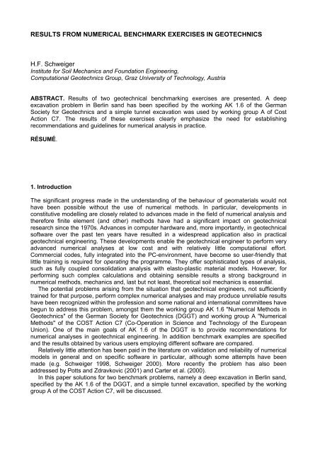
RESULTS FROM NUMERICAL BENCHMARK EXERCISES IN GEOTECHNICS
H.F. Schweiger
Institute for Soil Mechanics and Foundation Engineering,
Computational Geotechnics Group, Graz University of Technology, Austria
ABSTRACT. Results of two geotechnical benchmarking exercises are presented. A deep
excavation problem in Berlin sand has been specified by the working AK 1.6 of the German
Society for Geotechnics and a simple tunnel excavation was used by working group A of Cost
Action C7. The results of these exercises clearly emphasize the need for establishing
recommendations and guidelines for numerical analysis in practice.
RÉSUMÉ.
1. Introduction
The significant progress made in the understanding of the behaviour of geomaterials would not
have been possible without the use of numerical methods. In particular, developments in
constitutive modelling are closely related to advances made in the field of numerical analysis and
therefore finite element (and other) methods have had a significant impact on geotechnical
research since the 1970s. Advances in computer hardware and, more importantly, in geotechnical
software over the past ten years have resulted in a widespread application also in practical
geotechnical engineering. These developments enable the geotechnical engineer to perform very
advanced numerical analyses at low cost and with relatively little computational effort.
Commercial codes, fully integrated into the PC-environment, have become so user-friendly that
little training is required for operating the programme. They offer sophisticated types of analysis,
such as fully coupled consolidation analysis with elasto-plastic material models. However, for
performing such complex calculations and obtaining sensible results a strong background in
numerical methods, mechanics and, last but not least, theoretical soil mechanics is essential.
The potential problems arising from the situation that geotechnical engineers, not sufficiently
trained for that purpose, perform complex numerical analyses and may produce unreliable results
have been recognized within the profession and some national and international committees have
begun to address this problem, amongst them the working group AK 1.6 "Numerical Methods in
Geotechnics" of the German Society for Geotechnics (DGGT) and working group A "Numerical
Methods" of the COST Action C7 (Co-Operation in Science and Technology of the European
Union). One of the main goals of AK 1.6 of the DGGT is to provide recommendations for
numerical analyses in geotechnical engineering. In addition benchmark examples are specified
and the results obtained by various users employing different software are compared.
Relatively little attention has been paid in the literature on validation and reliability of numerical
models in general and on specific software in particular, although some attempts have been
made (e.g. Schweiger 1998, Schweiger 2000). More recently the problem has also been
addressed by Potts and Zdravkovic (2001) and Carter et al. (2000).
In this paper solutions for two benchmark problems, namely a deep excavation in Berlin sand,
specified by the AK 1.6 of the DGGT, and a simple tunnel excavation, specified by the working
group A of the COST Action C7, will be discussed.

2. Undrained analysis of a shield tunnel excavation
2.1. Specification of problem
This example has been specified by the Working Group A of COST Action C7 and has been
deliberately chosen very simple (e.g. constant undrained shear strength instead of increasing with
depth). Undrained conditions are considered and 3 analyses should be performed in terms of total
stresses in plane strain conditions:
Analysis A: elastic, no lining, uniform initial stress state
Analysis B: elastic-perfectly plastic, no lining, K o = 1.0
Analysis C: elastic-perfectly plastic, segmental lining, K o = 1.0, given ground loss
The tunnel diameter is given as 10 m and the overburden (measured from crown to surface) is
assumed to be 15 m. At a depth of 45 m below surface bedrock can be assumed (see Figure 1).
The material parameters for all analysis are given in Table 1.
Table 1. Material parameters for analyses A, B and C
Analysis γ G ν σ v = σ h (K o =1.0) c u E lining ν lining γ lining
kN/m 3 kPa - kPa kPa kPa - kN/m 3
A 20.0 12 000 0.495 - 400 - - - -
B 20.0 12 000 0.495 (z 130 - - -
C 20.0 12 000 0.495 (z 60 2.1 x 10 7 0.18 24.0
Computational step to be performed:
Analyses A and B: full excavation
Analysis C: full excavation with assumed ground loss of 2%
0.0 m surface
A
15 m
z
tunnel diameter = 10 m
B
thickness of lining = 0.3 m
D
C
-45.0 m bedrock
Figure 1. Geometry for benchmark shield tunnel
2.2 Results
Some selected results are presented in the following. 12 solutions (termed ST1 to ST12
respectively) have been submitted. Table 2 summarizes calculated displacements at various

locations which are indicated in Figure 1. It follows that there is a 20% difference of maximum
settlement of point A, which is by no means acceptable for an elastic solution. As will be seen
later this is entirely due to the different assumptions for the lateral boundary condition.
Table 2. Analysis A - calculated displacements of points A, B, C and D [mm]
A B C D vert. D horiz.
ST1 -50 -115 62 -24 -80
ST2 -48 -110 64 -21 -79
ST3 -53 -116 62 -25 -79
ST4 -46 -111 67 -20 -82
ST5 -56 -118 60 -27 -79
ST6 -51 -115 62 -26 -81
ST7 -48 -114 63 -24 -83
ST8 -48 -114 63 -24 -83
ST9 -45 -111 62 -22 -82
ST10 -44 -110 68 -19 -83
ST11 -50 -115 62 -24 -80
ST12 -47 -114 63 -24 -83
Figures 2 and 3 show settlements and horizontal displacements at the surface for the plastic
solution with constant undrained shear strength (Analysis B). In Figure 2 a similar scatter as in
Analysis A is observed with the exception of ST4, ST9 and ST10 which show an even larger
deviation from the "mean" of all analyses submitted. ST5 restrained vertical displacements at the
lateral boundary and thus the settlement is zero here. ST9 used a Von-Mises and not a Tresca
failure criterion which accounts for the difference. The strong influence of employing a Von-Mises
criterion as follows from Figure 2 has been verified by separate studies. It is emphasized
therefore that a careful choice of the failure criterion is essential in a non-linear analysis even for
a simple problem as considered here. The significant variation in predicted horizontal
displacements, mainly governed by the placement of the lateral boundary condition, is evident
from Figure 3. Taking the settlement at the surface above the tunnel axis (point A) the minimum
and maximum value calculated is 76 mm and 159 mm respectively. Thus differences are - as
expected - significantly larger than in the elastic case and again not acceptable.
distance from tunnel axis [m]
0 10 20 30 40 50 60 70 80 90 100
0
-20
vertical displacements [mm]
-40
-60
-80
-100
-120
-140
-160
ST1
ST3
ST4
ST5
ST6
ST7
ST8
ST9
ST10
ST11
ST12
-180
Figure 2. Calculated surface settlements - analysis B

distance from tunnel axis [m]
0 10 20 30 40 50 60 70 80 90 100
0
-5
horizontal displacements [mm]
-10
-15
-20
-25
-30
-35
-40
-45
-50
-55
ST1
ST3
ST4
ST5
ST6
ST7
ST8
ST9
ST10
ST11
ST12
-60
Figure 3. Calculated horizontal displacements at surface - analysis B
Figure 4 plots surface settlements for the elastic-perfectly plastic analysis with a specified volume
loss of 2% and the even wide scatter in results is indeed not very encouraging. The significant
effect of the vertically and horizontally restrained boundary condition used in ST5 is apparent.
However in the other solutions no obvious cause for the differences could be found except that
the lateral boundary has been placed at different distances from the symmetry axes and that the
specified volume loss is modelled in different ways. The range of calculated values for the surface
settlement above the tunnel axis is between 1 and 25 mm and for the crown settlement between
17 and 45 mm respectively. The normal forces in the lining and the contact pressure between soil
and lining do not differ that much (variation is within 15 and 20% respectively), with the exception
of ST9 who calculated significantly lower values.
distance from tunnel axis [m]
0 10 20 30 40 50 60 70 80 90 100
5
0
vertical displacements [mm]
-5
-10
-15
-20
-25
-30
-35
ST1
ST2
ST3
ST4
ST5
ST6
ST8
ST9
ST10
ST11
ST12
-40
Figure 4. Calculated surface settlements - analysis C
After comparing all results submitted, a second round of calculations has been performed. All
authors were asked to redo their analysis with the lateral boundary placed at a distance of 100 m
from the tunnel axis with horizontal displacements restrained. By doing so all solutions for
analyses A and B were within acceptable limits, for analysis C however, still significant
differences in results were obtained, although the range of scatter was reduced (Figure 5). These
differences are most likely due to the way different software handles the specified volume loss.
Again this is a strong case for developing guidelines and reference examples how to model this
(and other) excavation problems.

distance from tunnel axis [m]
0
0 10 20 30 40 50 60 70 80 90 100
vertical displacements [mm]
-5
-10
-15
-20
ST1
ST3
ST5
ST7
ST8
ST9
ST10
-25
Figure 5. Calculated surface settlements - analysis C with lateral boundary at 100 m
3. Deep excavation
3.1. Geometry, basic assumptions and computational steps
The general layout of the problem follows from Figure 6 and the following additional specifications
have been given:
- plane strain
- influence of diaphragm wall construction is neglected, i.e. initial stresses are calculated
without the wall, then wall is "wished-in-place"
- diaphragm wall modelling: beam elements or continuum elements
(E b = 30.0e6 kPa, ν = 0.15, d = 0.8 m)
- interface elements between wall and soil
- horizontal hydraulic cut off at -30.00 m is not considered as structural support, the same
mechanical properties as for the surrounding soil are assumed
- hydrostatic water pressures correspond to water levels inside and outside excavation
(groundwater lowering is performed in one step before excavation starts)
- anchors are modelled as rods, the grouted body as membrane element which guarantee a
continuous load transfer to the soil
- given anchor forces in Figure 1 are design loads
Computational steps to be performed:
stage 0: initial stress state (given by σ' v = γz, σ' h = K o γz, K o = 0.43)
stage 1: activation of diaphragm wall and groundwater lowering to -17.90 m
stage 2: excavation step 1 (to level -4.80 m)
stage 3: activation of anchor 1 at level -4.30 m and prestressing
stage 4: excavation step 2 (to level -9.30 m)
stage 5: activation of anchor 2 at level -8.80 m and prestressing
stage 6: excavation step 3 (to level -14.35 m)
stage 7: activation of anchor 3 at level -13.85 m and prestressing
stage 8: excavation step 4 (to level -16.80 m)
Distance and prestressing loads for anchors follow from Figure 6.

z
x
30 m
excavation step 1 = - 4.80m
excavation step 2 = - 9.30m
2 - 3 x width of excavation
0.00m
GW = -3.00m below surface
27°
27°
19.8m
8.0m
excavation step 3 = -14.35m
excavation step 4 = -16.80m
-17.90m
27°
23.3m
23.8m
8.0m
8.0m
top of hydraulic barrier = -30.00m
-32.00m = base of diaphragm wall
2 - 3 x width of excavation
γ'=γ' sand
Specification for anchors:
prestressed anchor force: 1. row: 768KN
2. row: 945KN
3. row: 980KN
distance of anchors: 1. row: 2.30m
2. row: 1.35m
3. row: 1.35m
cross section area: 15 cm 2
Young's modulus E = 2.1 e8 kN/m 2
sand
0.8m
Figure 6. Geometry and excavation stages
3.2. Material parameters
Some reference values for stiffness and strength parameters from the literature, frequently used
in the design of excavations in Berlin sand, were given (z = depth below surface):
E s ≈ 20 000 √z kPa
E s ≈ 60 000 √z kPa
ϕ = 35°
γ = 19 kN/m 3
γ' = 10 kN/m 3
K o = 1 – sin ϕ
for 0 < z < 20 m
for z > 20 m
(medium dense)
In addition to these values from literature, results from oedometer tests (on loose and dense
samples) and triaxial tests (confining pressures σ 3 = 100, 200 and 300 kPa) have been provided.
It was not possible to include a significantly large number of test results and thus the question
arose whether the stiffness values obtained from the oedometer test have been representative. If,
for example, the constitutive model requires a tangential oedometric stiffness at a reference
pressure of 100 kPa as an input parameter, a value of only Es ≈ 12 000 kPa was found based on
these experiments. If a secant modulus for a pressure range beyond 200 kPa is determined a
value of about 40 000 kPa is obtained. This was considered as too low by many authors and
indeed other test results from Berlin sand in the literature indicate higher values. For example
from Ohde (1951) values of about 35 000 to 45 000 kPa could be estimated as reference loading
modulus of a medium dense sand at a reference pressure of 100 kPa.
Properties for the diaphragm wall (linear elastic):
E = 30 000 x 10 3 kPa
ν = 0.15
γ = 24 kN/m 3

3.3. Comments on solutions submitted
A wide variety of programmes and constitutive models has been employed to solve this problem.
Simple elastic-perfectly plastic material models such as the Mohr-Coulomb or Drucker-Prager
failure criterion (B1, B4, B5, B6, B7, B9, B12 and B16), still widely used in practice have been
chosen by a number of authors. Several entries utilized the computer code PLAXIS (Brinkgreve &
Vermeer 1998) with the so-called Hardening Soil model. One submission used a similar plasticity
model with a simplified small strain stiffness formulation for the elastic range (B14). Three entries
employed a hypoplastic formulation (B3, B3a and B13), B3 without and B3a and B13 with
considering intergranular strains (Niemunis & Herle 1997).
Only marginal differences exist in the assumptions of strength parameters (everybody trusted
the experiments in this respect), the angle of internal friction ϕ was taken as 36° or 37° and a
small cohesion was assumed to increase numerical stability by some authors. A significant
variation was observed however in the assumption of the dilatancy angle ψ, ranging from 0° to
15°.
For reasons mentioned earlier only a limited number of analysts used the provided laboratory
test results to calibrate their material model. Most of the analysts used data from the literature
from Berlin sand or their own experience to arrive at input parameters for their analysis assuming
an increase with depth either by introducing some sort of power law or by defining different layers
with different (constant) Young's moduli. However the choice of the reference moduli for primary
loading and unloading/reloading varied significantly. Additional variation was introduced through
different formulations for interface elements (zero thickness, finite thickness), element types
(linear, quadratic), domains analysed (the width of meshes varied from 80 to 160 m, the depth
from 50 to 160 m), modelling of the prestressed anchors, implementation details of constitutive
models and the solution procedure with respective convergence criteria. The latter aspect is
commonly ignored in practice but it can be easily shown that it may have a significant influence
not only for stress levels near failure but also for working load conditions (Potts and Zdravkovic,
1999).
3.4. Selected results
Because some of the analyses made extremely unrealistic assumptions for the material
parameters (B2, B3, B7, B9 and B17), they have been excluded for the comparison presented in
the following.
Figure 7a depicts lateral displacements of the diaphragm wall due to lowering of the
groundwater level inside the excavation pit to -17.90 m below surface. No clear trend e.g. with
respect to the constitutive model could be identified, B6 is an elastic-perfectly plastic model but so
is B16, both on the opposite sides of the range of results. Observing this variety of results already
in the first construction stage, it is of course not surprising that the scatter increases with further
calculation steps which will be shown later. It should be emphasized at this stage that not only the
assumption of the constitutive model and the parameters have a significant influence on the result
of this construction stage but also the way the groundwater lowering is simulated in the numerical
analysis. Programme specific implementation details, the commercial user of a particular software
may not be aware of, will contribute to the differences shown in Figure 7a. Because of these
possible differences in modelling the groundwater lowering depending on the software used, it
was investigated whether a more clear picture would evolve if a construction stage without the
influence of the groundwater lowering is considered. For that purpose the wall deflection for
excavation step 1 (to -4.80 m below surface) was plotted setting displacements to zero before this
construction stage. The result follows from Figure 7b and the significant scatter already at this
stage is obvious. Although most of the differences can be attributed to the stiffness parameters
chosen as input, a few additional conclusions can be drawn. The largest horizontal displacement
is obtained from the hypoplastic analysis, which was not the case in the previous construction
stage (groundwater lowering). This indicates the strong response of these models on the stress
paths, which are obviously quite different for these two construction steps. This effect of different
stress paths is also observed in the other models but by far not to the same extent. The elasticplastic
models with stress dependent stiffness (B2a, B8, B10 and B14) tend to give smaller

displacements compared to the elastic-perfectly plastic models. Exceptions are B5 and B16,
which show a distinctly different deflection curve although the Young's modulus chosen is similar
to other entries. Most probably is due to the fact that they did not use an interface element for
modelling the soil/wall interaction.
-40 -35 -30 -25 -20 -15 -10 -5 0 5
0
2
4
6
8
10
-60 -55 -50 -45 -40 -35 -30 -25 -20 -15 -10 -5 0 5 10
0
2
4
6
8
10
B1
B2a
B4
B5
B6
B8
B9
B10
B11
B12
B13
B14
B16
12
14
16
18
20
22
24
26
28
30
depth below surface [m]
B1
B2a
B4
B5
B6
B8
B9
B10
B11
B12
B13
B14
B16
12
14
16
18
20
22
24
26
28
30
depth below surface [m]
32
-40 -35 -30 -25 -20 -15 -10 -5 0 5
horizontal displacement [mm]
32
-60 -55 -50 -45 -40 -35 -30 -25 -20 -15 -10 -5 0 5 10
horizontal displacement [mm]
Figure 7. Wall deflection a) after groundwater lowering, b) for first excavation step
Limited in situ measurements are available for this project and although some simplifications
compared to the actual construction have been introduced for this benchmark exercise in order to
facilitate the calculations, the order of magnitude of displacements can be assumed to be known.
Figure 8 shows the measured wall deflection for the final construction stage together with
calculated values. It should be mentioned that measurements have been taken by inclinometer
readings, fixed at the base of the wall, but unfortunately no geodetic survey of the wall head is
available. It is very likely that the wall base moves horizontally and a parallel shift of the
measurement is thought to reflect the in situ behaviour more closely, and therefore the
measurement readings have been shifted by 10 mm in Figure 8. This is confirmed by other
measurements under similar conditions. The calculated maximum horizontal wall displacement
for all results considered varies between approximately 10 to 65 mm (exception B6). The shape
of the deflection curves is also quite different. Some results indicate the maximum displacement
slightly above the final excavation level, others show the maximum value at the top of the wall.

measurement
(corrected)
-80 -70 -60 -50 -40 -30 -20 -10 0 10
0
2
4
6
8
10
B1
B2a
B4
B5
B6
B8
B9
B10
B11
B12
B13
B14
B15
B16
measurement
(corrected)
12
14
16
18
20
22
24
26
28
30
depth below surface [m]
32
-80 -70 -60 -50 -40 -30 -20 -10 0 10
horizontal displacement [mm]
Figure 8. Calculated wall deflections after final excavation step
distance from wall [m]
20
0 10 20 30 40 50 60 70 80 90 100
vertical displacement of surface [mm]
10
0
-10
-20
-30
-40
-50
B1
B2a
B4
B5
B6
B8
B9
B10
B11
B12
B13
B14
B15
B16
Figure 9. Calculated surface settlements after final excavation step

When comparing the results of the calculations with the measurements it has to be pointed out
that the simplification introduced in modelling the groundwater lowering (one step lowering
instead of step-wise lowering according to the excavation progress) leads to higher horizontal
displacements. Further studies revealed that the difference in calculated horizontal displacements
due to the difference in modelling the groundwater lowering is strongly dependent on the
constitutive law employed and ranges in the order of 5 to 15 mm. This may be one of the reasons
why B15, which is an elastic-plastic analysis with stepwise groundwater lowering, is close to the
measurement, but it also means that all solutions predicting less than 30 mm of horizontal
displacement are far off reality.
Figure 9 depicts the calculated surface settlements. Settlements of 45 mm (B11) have to be
compared with a heave of about 15 mm (B4). Considering the fact that calculation of surface
settlements is one of the main goals of such an analysis these results are not very encouraging.
4. Conclusion
Results from a geotechnical benchmark exercise have been presented. A typical problem of a
deep excavation in Berlin sand, formulated by the working group 1.6 of the German Society for
Geotechnics, has been solved by a number of geotechnical engineers from universities and
consulting companies utilizing different finite element codes and constitutive models. The
comparison of the solutions submitted showed a wide scatter in results and only the most
extreme solutions on the far end of the range could be explained with respect to assumptions of
input parameters made in the analysis. Some of the results showed obvious errors such as
incorrect prestress forces of anchors but most analyses made reasonable assumptions for
parameters, discretisation and other modelling details.
This benchmark exercise demonstrates the strong need for guidelines and recommendations
how to model typical geotechnical problems in practice. Pitfalls and unrealistic modelling
assumptions, the commercial user may not be aware of, have to be pointed out and procedures
have to be developed to identify these.
5. References
Brinkgreve R.B.J., Vermeer P.A. (1998), PLAXIS: Finite element code for soil and rock analyses, version 7.
Balkema.
Carter, J.P, Desai, C.S., Potts, D.M., Schweiger, H.F. & S.W. Sloan 2000. Computing and Computer
Modelling in Geotechnical Engineering. Proc. GeoEng2000, Melbourne, Technomic Publishing,
Lancaster. (Vol. 1: invited papers), 1157-1252.
Niemunis, A. & I. Herle 1997. Hypoplastic model for cohesionless soils with elastic strain range. Mechanics
of cohesive-frictional materials, 2, 279-299.
Ohde, J. 1951. Grundbaumechanik (in German), Huette, BD. III, 27. Auflage.
Potts, D.M & L. Zdravkovic (1999). Finite element analysis in geotechnical engineering – Theory. Thomas
Telford
Potts, D.M & L. Zdravkovic (2001). Finite element analysis in geotechnical engineering – Application.
Thomas Telford
Schweiger, H. F. 1998. Results from two geotechnical benchmark problems. Proc. 4th European Conf.
Numerical Methods in Geotechnical Engineering, Cividini, A. (ed.), Springer, 645-654.
Schweiger, H. F. 2000. Ergebnisse des Berechnungsbeispieles Nr. 3 "3-fach verankerte Baugrube".
Tagungsband Workshop "Verformungsprognose für tiefe Baugruben", Stuttgart, 7-67. (in German)
REFERENCE:
Results from numerical benchmark exercises in geotechnics
Proc. 5th European Conf. Numerical Methods in Geotechnical Engineering, Presses Ponts et
chaussees, Paris, 2002, 305-314