3.7.8 Solving Linear Systems
3.7.8 Solving Linear Systems
3.7.8 Solving Linear Systems

You also want an ePaper? Increase the reach of your titles
YUMPU automatically turns print PDFs into web optimized ePapers that Google loves.
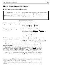
3.7 <strong>Linear</strong> Algebra 531<br />
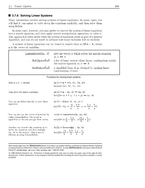
<strong>3.7.8</strong> <strong>Solving</strong> <strong>Linear</strong> <strong>Systems</strong><br />
Many calculations involve solving systems of linear equations. In many cases, you<br />
will nd it convenient to write down the equations explicitly, and then solve them<br />
using Solve.<br />
In some cases, however, you may prefer to convert the system of linear equations<br />
into a matrix equation, and then apply matrix manipulation operations to solve it.<br />
This approach is often useful when the system of equations arises as part of a general<br />
algorithm, and you do not know in advance how manyvariables will be involved.<br />
A system of linear equations can be stated in matrix form as M:x = b, where<br />
x is the vector of variables.<br />
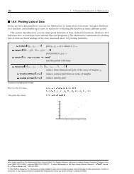
<strong>Linear</strong>Solve[m, b]<br />
NullSpace[m]<br />
RowReduce[m]<br />
give thevector x which solves the matrix equation<br />
m.x == b<br />
a list of basis vectors whose linear combinations satisfy<br />
the matrix equation m.x == 0<br />
a simplied form of m obtained by making linear<br />
combinations of rows<br />
Functions for solving linear systems.<br />
Here is a 2 2 matrix. In[1]:= m = {{1, 5}, {2, 1}}<br />
Out[1]= {{1, 5}, {2, 1}}<br />
This gives two linear equations. In[2]:= m . {x, y} == {a, b}<br />
Out[2]= {x + 5 y, 2 x + y} == {a, b}<br />
You can use Solve directly to solve these<br />
equations.<br />
In[3]:= Solve[ %, {x, y} ]<br />
-a 5 b 2 a b<br />
Out[3]= {{x -> -- + ----, y -> ---- - -}}<br />
9 9 9 9<br />
You can also get the vector of solutions by<br />
calling <strong>Linear</strong>Solve. The result is<br />
equivalent to the one you get from Solve.<br />
In[4]:= <strong>Linear</strong>Solve[m, {a, b}]<br />
a 5 b -2 a b<br />
Out[4]= {-(- - ----), -( ------ + -)}<br />
9 9 9 9<br />
Another way to solve the equations is to<br />
invert the matrix m, and then multiply<br />
{a, b} by the inverse. This is not as<br />
ecient asusing<strong>Linear</strong>Solve.<br />
In[5]:= Inverse[m] . {a, b}<br />
-a 5 b 2 a b<br />
Out[5]= {--- + ----, ---- - -}<br />
9 9 9 9<br />
Web sample page from The Mathematica Book, First Edition, by Stephen Wolfram, published by Addison-Wesley Publishing<br />
Company (hardcover ISBN 0-201-19334-5; softcover ISBN 0-201-19330-2). To order Mathematica or this book contact Wolfram<br />
Research: info@wolfram.com; http://www.wolfram.com/; 1-800-441-6284.<br />
c 1988 Wolfram Research, Inc. Permission is hereby granted for web users to make one paper copy of this page for their<br />
personal use. Further reproduction, or any copying of machine-readable files (including this one) to any server computer, is strictly<br />
prohibited.
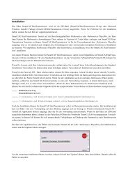
532 3. Advanced Mathematics in Mathematica<br />
Particularly when you have large, sparse, matrices, <strong>Linear</strong>Solve is the most<br />
ecient method to use.<br />
If you have a square matrix m with a nonzero determinant, then you can always<br />
nd a unique solution to the matrix equation m:x = b for any b. If, however,<br />
the matrix m has determinant zero, then there can be no vector x which satises<br />
m:x = b for a particular b. This situation corresponds to the case in which the<br />
linear equations embodied in m are not independent.<br />
When m has determinant zero, it is nevertheless always possible to nd vectors<br />
x that satisfy m:x = 0. The set of vectors x satisfying this equation form the<br />
null space or kernel of the matrix m. Any ofthevectors can be expressed as a<br />
linear combination of a particular set of basis vectors, which can be obtained using<br />
NullSpace[m].<br />
Here is a simple matrix, corresponding to<br />
two identical linear equations.<br />
In[6]:= m = {{1, 2}, {1, 2}}<br />
Out[6]= {{1, 2}, {1, 2}}<br />
The matrix has determinant zero. In[7]:= Det[ m ]<br />
Out[7]= 0<br />
<strong>Linear</strong>Solve cannot nd a solution to the<br />
equation m:x = b in this case.<br />
In[8]:= <strong>Linear</strong>Solve[m, {a, b}]<br />
<strong>Linear</strong>Solve::nsl:<br />
<strong>Linear</strong> equation encountered which has no solution.<br />
Out[8]= <strong>Linear</strong>Solve[{{1, 2}, {1, 2}}, {a, b}]<br />
There is a single basis vector for the null<br />
space of m.<br />
In[9]:= NullSpace[ m]<br />
Out[9]= {{-2, 1}}<br />
Multiplying the basis vector for the null<br />
space by m gives the zero vector.<br />
Here is a simple symbolic matrix with<br />
determinant zero.<br />
The basis for the null space of m contains<br />
two vectors. Any linear combination of<br />
these vectors gives zero when multiplied by<br />
m.<br />
In[10]:= m . %[[1]]<br />
Out[10]= {0, 0}<br />
In[11]:= m = {{a, b, c}, {2 a, 2 b, 2 c}, {3 a, 3 b, 3 c}}<br />
Out[11]= {{a, b, c}, {2 a, 2 b, 2 c}, {3 a, 3 b, 3 c}}<br />
In[12]:= NullSpace[ m ]<br />
c<br />
b<br />
Out[12]= {{-(-), 0, 1}, {-(-), 1, 0}}<br />
a<br />
a<br />
An important feature of <strong>Linear</strong>Solve and NullSpace is that they work with<br />
rectangular, aswell as square, matrices.<br />
Web sample page from The Mathematica Book, First Edition, by Stephen Wolfram, published by Addison-Wesley Publishing<br />
Company (hardcover ISBN 0-201-19334-5; softcover ISBN 0-201-19330-2). To order Mathematica or this book contact Wolfram<br />
Research: info@wolfram.com; http://www.wolfram.com/; 1-800-441-6284.<br />
c 1988 Wolfram Research, Inc. Permission is hereby granted for web users to make one paper copy of this page for their<br />
personal use. Further reproduction, or any copying of machine-readable files (including this one) to any server computer, is strictly<br />
prohibited.
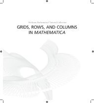
3.7 <strong>Linear</strong> Algebra 533<br />
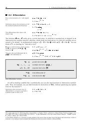
When you represent a system of linear equations by a matrix equation of the<br />
form m:x = b, the number of columns in m gives the number of variables, and the<br />
number of rows give the number of equations. There are a number of cases.<br />
Underdetermined<br />
Overdetermined<br />
Nonsingular<br />
Consistent<br />
Inconsistent<br />
number of independent equations less than the number<br />
of variables many solutions may exist<br />
number of independent equations more than the<br />
numberofvariables solutions may not exist<br />
number of independent equations equal to the number<br />
of variables, and determinant nonzero a unique<br />
solution exists<br />
at least one solution exists<br />
no solutions exist<br />
Classes of linear systems represented by rectangular matrices.<br />
This asks for the solution to the inconsistent<br />
set of equations x =1andx =0.<br />
In[13]:= <strong>Linear</strong>Solve[{{1}, {1}}, {1, 0}]<br />
<strong>Linear</strong>Solve::nsl:<br />
<strong>Linear</strong> equation encountered which has no solution.<br />
Out[13]= <strong>Linear</strong>Solve[{{1}, {1}}, {1, 0}]<br />
This matrix represents two equations, for<br />
three variables.<br />
In[14]:= m = {{1, 3, 4}, {2, 1, 3}}<br />
Out[14]= {{1, 3, 4}, {2, 1, 3}}<br />
<strong>Linear</strong>Solve gives one of the possible<br />
solutions to this underdetermined set of<br />
equations.<br />
When a matrix represents an<br />
underdetermined system of equations, the<br />
matrix has a non-trivial null space. In this<br />
case, the null space is spanned by a single<br />
vector.<br />
If you take the solution you get from<br />
<strong>Linear</strong>Solve, and add any linear<br />
combination of the basis vectors for the<br />
null space, you still get a solution.<br />
In[15]:= v = <strong>Linear</strong>Solve[m, {1, 1}]<br />
2 1<br />
Out[15]= {-, -, 0}<br />
5 5<br />
In[16]:= NullSpace[m]<br />
Out[16]= {{-1, -1, 1}}<br />
In[17]:= m . (v + 4 %[[1]])<br />
Out[17]= {1, 1}<br />
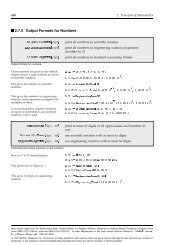
You can nd out the number of redundant equations corresponding to a particular<br />
matrix by evaluating Length[NullSpace[m]]. Subtracting this quantity from<br />
Web sample page from The Mathematica Book, First Edition, by Stephen Wolfram, published by Addison-Wesley Publishing<br />
Company (hardcover ISBN 0-201-19334-5; softcover ISBN 0-201-19330-2). To order Mathematica or this book contact Wolfram<br />
Research: info@wolfram.com; http://www.wolfram.com/; 1-800-441-6284.<br />
c 1988 Wolfram Research, Inc. Permission is hereby granted for web users to make one paper copy of this page for their<br />
personal use. Further reproduction, or any copying of machine-readable files (including this one) to any server computer, is strictly<br />
prohibited.
534 3. Advanced Mathematics in Mathematica<br />
the number of columns in m gives the rank of the matrix m.<br />
Web sample page from The Mathematica Book, First Edition, by Stephen Wolfram, published by Addison-Wesley Publishing<br />
Company (hardcover ISBN 0-201-19334-5; softcover ISBN 0-201-19330-2). To order Mathematica or this book contact Wolfram<br />
Research: info@wolfram.com; http://www.wolfram.com/; 1-800-441-6284.<br />
c 1988 Wolfram Research, Inc. Permission is hereby granted for web users to make one paper copy of this page for their<br />
personal use. Further reproduction, or any copying of machine-readable files (including this one) to any server computer, is strictly<br />
prohibited.