Mathematica Tutorial: Visualization And Graphics - Wolfram Research

Wolfram Mathematica Tutorial Collection 

Visualization and Graphics

For use with Wolfram Mathematica ® 7.0 and later. 

For the latest updates and corrections to this manual: 

visit reference.wolfram.com 

For information on additional copies of this documentation: 

visit the Customer Service website at www.wolfram.com/services/customerservice 

or email Customer Service at info@wolfram.com 

Comments on this manual are welcomed at: 

comments@wolfram.com 

Printed in the United States of America. 

15 14 13 12 11 10 9 8 7 6 5 4 3 2 

©2008 Wolfram Research, Inc. 

All rights reserved. No part of this document may be reproduced or transmitted, in any form or by any means, 

electronic, mechanical, photocopying, recording or otherwise, without the prior written permission of the copyright 

holder. 

Wolfram Research is the holder of the copyright to the Wolfram Mathematica software system ("Software") described 

in this document, including without limitation such aspects of the system as its code, structure, sequence, 

organization, “look and feel,” programming language, and compilation of command names. Use of the Software 

unless pursuant to the terms of a license granted by Wolfram Research or as otherwise authorized by law is an 

infringement of the copyright. 

Wolfram Research, Inc. and Wolfram Media, Inc. ("Wolfram") make no representations, express, 

statutory, or implied, with respect to the Software (or any aspect thereof), including, without limitation, 

any implied warranties of merchantability, interoperability, or fitness for a particular purpose, all of which 

are expressly disclaimed. Wolfram does not warrant that the functions of the Software will meet your 

requirements or that the operation of the Software will be uninterrupted or error free. As such, Wolfram 

does not recommend the use of the software described in this document for applications in which errors 

or omissions could threaten life, injury or significant loss. 

Mathematica, MathLink, and MathSource are registered trademarks of Wolfram Research, Inc. J/Link, MathLM, 

.NET/Link, and webMathematica are trademarks of Wolfram Research, Inc. Windows is a registered trademark of 

Microsoft Corporation in the United States and other countries. Macintosh is a registered trademark of Apple 

Computer, Inc. All other trademarks used herein are the property of their respective owners. Mathematica is not 

associated with Mathematica Policy Research, Inc.

Contents 

Graphics and Sound 

Basic Plotting . . . . . . . . . . . . . . . . . . . . . . . . . . . . . . . . . . . . . . . . . . . . . . . . . . . . . . . . . . . . . . . . . . . 1 

Options for Graphics . . . . . . . . . . . . . . . . . . . . . . . . . . . . . . . . . . . . . . . . . . . . . . . . . . . . . . . . . . . . 2 

Redrawing and Combining Plots . . . . . . . . . . . . . . . . . . . . . . . . . . . . . . . . . . . . . . . . . . . . . . . . 9 

Manipulating Options . . . . . . . . . . . . . . . . . . . . . . . . . . . . . . . . . . . . . . . . . . . . . . . . . . . . . . . . . . . 14 

Three-Dimensional Surface Plots . . . . . . . . . . . . . . . . . . . . . . . . . . . . . . . . . . . . . . . . . . . . . . . 16 

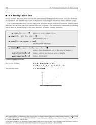
Plotting Lists of Data . . . . . . . . . . . . . . . . . . . . . . . . . . . . . . . . . . . . . . . . . . . . . . . . . . . . . . . . . . . 22 

Parametric Plots . . . . . . . . . . . . . . . . . . . . . . . . . . . . . . . . . . . . . . . . . . . . . . . . . . . . . . . . . . . . . . . . 25 

Some Special Plots . . . . . . . . . . . . . . . . . . . . . . . . . . . . . . . . . . . . . . . . . . . . . . . . . . . . . . . . . . . . . 29 

Sound . . . . . . . . . . . . . . . . . . . . . . . . . . . . . . . . . . . . . . . . . . . . . . . . . . . . . . . . . . . . . . . . . . . . . . . . . . 31 

The Structure of Graphics and Sound 

The Structure of Graphics . . . . . . . . . . . . . . . . . . . . . . . . . . . . . . . . . . . . . . . . . . . . . . . . . . . . . . . 33 

Two-Dimensional Graphics Elements . . . . . . . . . . . . . . . . . . . . . . . . . . . . . . . . . . . . . . . . . . . . 39 

Graphics Directives and Options . . . . . . . . . . . . . . . . . . . . . . . . . . . . . . . . . . . . . . . . . . . . . . . . 45 

Coordinate Systems for Two-Dimensional Graphics . . . . . . . . . . . . . . . . . . . . . . . . . . . . . 51 

Labeling Two-Dimensional Graphics . . . . . . . . . . . . . . . . . . . . . . . . . . . . . . . . . . . . . . . . . . . . 60 

Insetting Objects in Graphics . . . . . . . . . . . . . . . . . . . . . . . . . . . . . . . . . . . . . . . . . . . . . . . . . . . 64 

Density and Contour Plots . . . . . . . . . . . . . . . . . . . . . . . . . . . . . . . . . . . . . . . . . . . . . . . . . . . . . . 67 

Three-Dimensional Graphics Primitives . . . . . . . . . . . . . . . . . . . . . . . . . . . . . . . . . . . . . . . . . 71 

Three-Dimensional Graphics Directives . . . . . . . . . . . . . . . . . . . . . . . . . . . . . . . . . . . . . . . . . 76 

Coordinate Systems for Three-Dimensional Graphics . . . . . . . . . . . . . . . . . . . . . . . . . . . . 81 

Lighting and Surface Properties . . . . . . . . . . . . . . . . . . . . . . . . . . . . . . . . . . . . . . . . . . . . . . . . . 89 

Labeling Three-Dimensional Graphics . . . . . . . . . . . . . . . . . . . . . . . . . . . . . . . . . . . . . . . . . . . 96 

Efficient Representation of Many Primitives . . . . . . . . . . . . . . . . . . . . . . . . . . . . . . . . . . . . . 100 

Formats for Text in Graphics . . . . . . . . . . . . . . . . . . . . . . . . . . . . . . . . . . . . . . . . . . . . . . . . . . . . 103 

Graphics Primitives for Text . . . . . . . . . . . . . . . . . . . . . . . . . . . . . . . . . . . . . . . . . . . . . . . . . . . . 106 

The Representation of Sound . . . . . . . . . . . . . . . . . . . . . . . . . . . . . . . . . . . . . . . . . . . . . . . . . . . 108 

Exporting Graphics and Sounds . . . . . . . . . . . . . . . . . . . . . . . . . . . . . . . . . . . . . . . . . . . . . . . . . 110 

Importing Graphics and Sounds . . . . . . . . . . . . . . . . . . . . . . . . . . . . . . . . . . . . . . . . . . . . . . . . 113

Editing Mathematica Graphics 

Introduction . . . . . . . . . . . . . . . . . . . . . . . . . . . . . . . . . . . . . . . . . . . . . . . . . . . . . . . . . . . . . . . . . . . . 115 

Drawing Tools . . . . . . . . . . . . . . . . . . . . . . . . . . . . . . . . . . . . . . . . . . . . . . . . . . . . . . . . . . . . . . . . . . 118 

Selecting Graphics Objects . . . . . . . . . . . . . . . . . . . . . . . . . . . . . . . . . . . . . . . . . . . . . . . . . . . . . . 128 

Reshaping Graphics Objects . . . . . . . . . . . . . . . . . . . . . . . . . . . . . . . . . . . . . . . . . . . . . . . . . . . . 138 

Resizing, Cropping, and Adding Margins to Graphics . . . . . . . . . . . . . . . . . . . . . . . . . . . . 160 

Graphics as Input . . . . . . . . . . . . . . . . . . . . . . . . . . . . . . . . . . . . . . . . . . . . . . . . . . . . . . . . . . . . . . . 163 

Interacting with 3D Graphics . . . . . . . . . . . . . . . . . . . . . . . . . . . . . . . . . . . . . . . . . . . . . . . . . . . 164

Graphics and Sound 

Basic Plotting 

Plot@ f ,8x,x min ,x max

2 Visualization and Graphics 

In[4]:= 

You can give a list of functions to plot. A different color will automatically be used for each 

function. 

Plot@8Sin@xD, Sin@2 xD, Sin@3 xD

Visualization and Graphics 3 

Plot@ f ,8x,x min ,x max valueD 

make a plot, specifying a particular value for an option 

Choosing an option for a plot. 

A function like Plot has many options that you can set. Usually you will need to use at most a 

few of them at a time. If you want to optimize a particular plot, you will probably do best to 

experiment, trying a sequence of different settings for various options. 

Each time you produce a plot, you can specify options for it. "Redrawing and Combining Plots" 

will also discuss how you can change some of the options, even after you have produced the 

plot. 

option name 

default value 

AspectRatio 1ëGoldenRatio the height-to-width ratio for the plot; 

Automatic sets it from the absolute x and 

y coordinates 

Axes True whether to include axes 

AxesLabel None labels to be put on the axes; ylabel specifies 

a label for the y axis, 8xlabel, ylabel< for 

both axes 

AxesOrigin Automatic the point at which axes cross 

BaseStyle 8< the default style to use for the plot 

FormatType 

TraditionalFoÖ 

the default format type to use for text in 

rm 

the plot 

Frame False whether to draw a frame around the plot 

FrameLabel None labels to be put around the frame; give a 

list in clockwise order starting with the 

lower x axis 

FrameTicks Automatic what tick marks to draw if there is a frame; 

None gives no tick marks 

GridLines None what grid lines to include; Automatic 

includes a grid line for every major tick 

mark 

PlotLabel None an expression to be printed as a label for 

the plot 

PlotRange Automatic the range of coordinates to include in the 

plot; All includes all points 

Ticks Automatic what tick marks to draw if there are axes; 

None gives no tick marks 

Some of the options for Plot. These can also be used in Show.


Here is a plot with all options having their default values. 

In[1]:= Plot@Sin@x^2D, 8x, 0, 3


In[5]:= 

Setting the AspectRatio option changes the whole shape of your plot. AspectRatio gives 

the ratio of width to height. Its default value is the inverse of the Golden Ratio~supposedly the 

most pleasing shape for a rectangle. 

Plot@Sin@x^2D, 8x, 0, 3 1D 

1.0 

0.5 

Out[5]= 

0.5 1.0 1.5 2.0 2.5 3.0 

-0.5 

-1.0 

Automatic 

None 

All 

True 

False 

use internal algorithms 

do not include this 

include everything 

do this 

do not do this 

Some common settings for various options. 

When Mathematica makes a plot, it tries to set the x and y scales to include only the 

“interesting” parts of the plot. If your function increases very rapidly, or has singularities, the 

parts where it gets too large will be cut off. By specifying the option PlotRange, you can control 

exactly what ranges of x and y coordinates are included in your plot. 

Automatic 

All 

8y min ,y max < 

8xrange,yrange< 

show at least a large fraction of the points, including the 

“interesting” region (the default setting) 

show all points 

show a specific range of y values 

show the specified ranges of x and y values 

Settings for the option PlotRange.


In[6]:= 

The setting for the option PlotRange gives explicit y limits for the graph. With the y limits 

specified here, the bottom of the curve is cut off. 

Plot@Sin@x^2D, 8x, 0, 3 80, 1.2 0. Mathematica tries to sample more points 

x 

in the region where the function wiggles a lot, but it can never sample the infinite number that 

you would need to reproduce the function exactly. As a result, there are slight glitches in the 

plot. 

In[7]:= Plot@Sin@1 ê xD, 8x, -1, 1


Filling None filling to insert under each curve 

FillingStyle Automatic style to use for filling 

PlotPoints 50 the initial number of points at which to 

sample the function 

MaxRecursion Automatic the maximum number of recursive subdivi - 

sions allowed 

More options for Plot. These cannot be used in Show. 

This uses PlotStyle to specify a dashed curve. 

In[8]:= 

Plot@Sin@x^2D, 8x, 0, 3


By default nothing is indicated when the PlotRange is set, so that it cuts off curves. 

In[11]:= Plot@8Sin@x^2D, Cos@x^2D


In[15]:= 

The filling can be specified to extend to an arbitrary height, such as the bottom of the graphic. 

Filling colors are automatically blended where they overlap. 

Plot@8Sin@xD, Cos@xD


Here is a simple plot. 

In[1]:= Plot@ChebyshevT@7, xD, 8x, -1, 1 8-1, 2 "A Chebyshev Polynomial"D 

A Chebyshev Polynomial 

2.0 

1.5 

Out[3]= 

1.0 

0.5 

-1.0 -0.5 0.5 1.0 

-0.5 

-1.0 

By using Show with a sequence of different options, you can look at the same plot in many 

different ways. You may want to do this, for example, if you are trying to find the best possible 

setting of options. 

You can also use Show to combine plots. All of the options for the resulting graphic will be based 

upon the options of the first graphic in the Show expression.


This sets gj0 to be a plot of J 0 HxL from x = 0 to 10. 

In[4]:= gj0 = Plot@BesselJ@0, xD, 8x, 0, 10


In[8]:= 

This replaces all instances of the symbol Line with the symbol Point in the graphics expression 

represented by gj0. 

gj0 ê. Line Ø Point 

1.0 

0.8 

0.6 

Out[8]= 

0.4 

0.2 

-0.2 

-0.4 

2 4 6 8 10 

Using Show@plot 1 , plot 2 , …D you can combine several plots into one. GraphicsGrid allows you 

to draw several plots in an array. 

GraphicsGrid@88plot 11 ,plot 12 ,…


In[10]:= 

If you redisplay an array of plots using Show, any options you specify will be used for the whole 

array, rather than for individual plots. 

Show@%, Frame -> True, FrameTicks -> NoneD 

Out[10]= 

1.0 

0.8 

0.6 

0.4 

0.2 

-0.2 

-0.4 

0.4 

0.2 

-0.2 

-0.4 

-0.6 

-0.8 

2 4 6 8 10 

4 6 8 10 

1.0 

0.5 

-0.5 

1.0 

0.5 

-0.5 

2 4 6 8 10 

2 4 6 8 10 

GraphicsGrid by default puts a narrow border around each of the plots in the array it gives. 

You can change the size of this border by setting the option Spacings -> 8h, v


Here is a simple plot. 

In[12]:= 

Plot@Cos@xD, 8x, -Pi, Pi 880, .005


Here is the default setting for the PlotRange option of Plot. 

In[1]:= 

Options@Plot, PlotRangeD 

Out[1]= 8PlotRange Ø 8Full, Automatic AllD; 

Until you explicitly reset it, the default for the PlotRange option will now be All. 

In[3]:= 

Options@Plot, PlotRangeD 

Out[3]= 8PlotRange Ø All< 

The graphics objects that you get from Plot or Show store information on the options they use. 

You can get this information by applying the Options function to these graphics objects. 

Options@plotD 

Options@plot,optionD 

AbsoluteOptions@plot,optionD 

show all the options used for a particular plot 

show the setting for a specific option 

show the absolute form used for a specific option, even if 

the setting for the option is Automatic or All 

Getting information on options used in plots. 

Here is a plot, with default settings for all options. 

In[4]:= g = Plot@SinIntegral@xD, 8x, 0, 20


While it is often convenient to use a variable to represent a graphic as in the above examples, 

the graphic itself can be evaluated directly. The typical ways to do this in the notebook interface 

are to copy and paste the graphic or to simply begin typing in the graphical output cell, at 

which point the output cell will be converted into a new input cell. 

When a plot created with no explicit ImageSize is placed into an input cell, it will automatically 

shrink to more easily accommodate input. 

The following input cell was created by copying and pasting the graphical output created in the 

previous example. 

1.5 

In[7]:= 

1.0 

AbsoluteOptionsB 

0.5 

, PlotRangeF 

5 10 15 20 

Out[7]= 9PlotRange Ø 994.08163 µ 10 -7 , 20.=, 94.08163 µ 10 -7 , 1.85194=== 

Three-Dimensional Surface Plots 

Plot3D@ f ,8x,x min ,x max


Three-dimensional graphics can be rotated in place by dragging the mouse inside of the 

graphic. Dragging inside of the graphic causes the graphic to tumble in a direction that follows 

the mouse, and dragging around the borders of the graphic causes the graphic to spin in the 

plane of the screen. Dragging the graphic while holding down the Shift key causes the graphic 

to pan. Use the Ctrl key (Cmd key on Macintosh) to zoom. 

There are many options for three-dimensional plots in Mathematica. Some are discussed here; 

others are described in "The Structure of Graphics and Sound". 

The first set of options for three-dimensional plots is largely analogous to those provided in the 

two-dimensional case. 

option name 

default value 

Axes True whether to include axes 

AxesLabel None labels to be put on the axes: zlabel specifies 

a label for the z axis, 

8xlabel, ylabel, zlabel< for all axes 

BaseStyle 8< the default style to use for the plot 

Boxed True whether to draw a three-dimensional box 

around the surface 

FaceGrids None how to draw grids on faces of the bounding 

box; All draws a grid on every face 

LabelStyle 8< style specification for labels 

Lighting Automatic simulated light sources to use 

Mesh Automatic whether an xy mesh should be drawn on 

the surface 

PlotRange 

9Full,Full, 

Automatic= 

the range of z or other values to include 

SphericalRegion False whether to make the circumscribing sphere 

fit in the final display area 

ViewAngle All angle of the field of view 

ViewCenter 81,1,1


FillingStyle Opacity@.5D style to use for filling 

PlotPoints 25 the number of points in each direction at 

which to sample the function; 9n x , n y = 

specifies different numbers in the x and y 

directions 

PlotStyle Automatic graphics directives for the style of each 

surface 

Some options for Plot3D. The first set can also be used in Show. 

In[2]:= 

This redraws the previous plot with options changed. With this setting for PlotRange, only the 

part of the surface in the range -0.5 § z § 0.5 is shown. 

Show@%, PlotRange -> 8-0.5, 0.5


Here is the same plot, with labels for the axes, and grids added to each face. 

In[5]:= 

Show@%, AxesLabel -> 8"Time", "Depth", "Value" AllD 

Out[5]= 

Probably the single most important issue in plotting a three-dimensional surface is specifying 

where you want to look at the surface from. The ViewPoint option for Plot3D and Show allows 

you to specify the point 8x, y, z< in space from which you view a surface. The details of how the 

coordinates for this point are defined are discussed in "Coordinate Systems for Three-Dimensional 

Graphics". When rotating a graphic using the mouse, you are adjusting the ViewPoint 

value. 

Here is a surface, viewed from the default view point 81.3, -2.4, 2


In[8]:= 

The ViewPoint option also accepts various symbolic values which represent common view 

points. 

Show@%, ViewPoint Ø AboveD 

Out[8]= 

81.3,-2.4,2< default view point 

Front 

Back 

Above 

Below 

Left 

Right 

in front, along the negative y direction 

in back, along the positive y direction 

above, along the positive z direction 

below, along the negative z direction 

left, along the negative x direction 

right, along the positive x direction 

Typical choices for the ViewPoint option. 

The human visual system is not particularly good at understanding complicated mathematical 

surfaces. As a result, you need to generate pictures that contain as many clues as possible 

about the form of the surface. 

View points slightly above the surface usually work best. It is generally a good idea to keep the 

view point close enough to the surface that there is some perspective effect. Having a box 

explicitly drawn around the surface is helpful in recognizing the orientation of the surface.


Here is a plot with the default settings for surface rendering options. 

In[9]:= Plot3D@Exp@-Hx^2 + y^2LD, 8x, -2, 2


In[12]:= 

The ColorFunction option by default uses Lighting -> "Neutral" so that the surface 

colors are not distorted by colored lights. 

Plot3D@8Sin@x yD


This plots the values. 

In[2]:= 

ListPlot@tD 

100 

80 

Out[2]= 

60 

40 

20 

2 4 6 8 10 

This joins the points with lines. 

In[3]:= 

ListLinePlot@tD 

100 

80 

Out[3]= 

60 

40 

20 

2 4 6 8 10 

In[4]:= 

When plotting multiple datasets, Mathematica chooses a different color for each dataset 

automatically. 

ListPlot@8t, 2 t


This plots the points. 

In[6]:= 

ListPlot@%D 

1400 

1200 

1000 

Out[6]= 

800 

600 

400 

200 

20 40 60 80 100 

In[7]:= 

This gives a rectangular array of values. The array is quite large, so we end the input with a 

semicolon to stop the result from being printed out. 

t3 = Table@Mod@x, yD, 8x, 30


Parametric Plots 

"Basic Plotting" described how to plot curves in Mathematica in which you give the y coordinate 

of each point as a function of the x coordinate. You can also use Mathematica to make parametric 

plots. In a parametric plot, you give both the x and y coordinates of each point as a function 

of a third parameter, say t. 

ParametricPlotA9 f x , f y =,9t,t min ,t max =E 

make a parametric plot 

ParametricPlotA99 f x , f y =,9g x ,g y =,…=,9t,t min ,t max =E 

plot several parametric curves together 

Functions for generating parametric plots. 

In[1]:= 

Here is the curve made by taking the x coordinate of each point to be Sin@tD and the y coordinate 

to be Sin@2 tD. 

ParametricPlot@8Sin@tD, Sin@2 tD


ParametricPlot3D@8 f x , f y , f z


This shows the same surface as before, but with the y coordinates distorted by a quadratic 

transformation. 

In[4]:= ParametricPlot3D@8u Sin@tD, u^2 Cos@tD, u


This produces a cylinder. Varying the t parameter yields a circle in the x-y plane, while varying 

u moves the circles in the z direction. 

In[6]:= ParametricPlot3D@8Sin@tD, Cos@tD, u


in which all or part of your surface is covered more than once. Such multiple coverings often 

lead to discontinuities in the mesh drawn on the surface, and may make ParametricPlot3D 

take much longer to render the surface. 

Some Special Plots 

As discussed in "The Structure of Graphics and Sound", Mathematica includes a full graphics 

programming language. In this language, you can set up many different kinds of plots. A few of 

the common ones are included in standard Mathematica packages. 

LogPlot@ f ,8x,x min ,x max


Here is a list of the first 10 primes. 

In[2]:= p = Table@Prime@nD, 8n, 10


Sound 

On most computer systems, Mathematica can produce not only graphics but also sound. Mathematica 

treats graphics and sound in a closely analogous way. 

For example, just as you can use Plot@ f , 8x, x min , x max


Play is set up so that the time variable that appears in it is always measured in absolute seconds. 

When a sound is actually played, its amplitude is sampled a certain number of times 

every second. You can specify the sample rate by setting the option SampleRate. 

PlayA f ,9t,0,t max =,SampleRate->rE 

play a sound, sampling it r times a second 

Specifying the sample rate for a sound. 

In general, the higher the sample rate, the better high-frequency components in the sound will 

be rendered. A sample rate of r typically allows frequencies up to rê2 hertz. The human auditory 

system can typically perceive sounds in the frequency range 20 to 22000 hertz (depending 

somewhat on age and sex). The fundamental frequencies for the 88 notes on a piano range 

from 27.5 to 4096 hertz. 

The standard sample rate used for compact disc players is 44100. The effective sample rate in 

a typical telephone system is around 8000. On most computer systems, the default sample rate 

used by Mathematica is around 8000. 

You can use Play@8 f 1 , f 2 , …D to produce stereo sound. In general, Mathematica supports any 

number of sound channels. 

ListPlayA8a 1 ,a 2 ,…rE 

play a sound with a sequence of amplitude levels 

Playing sampled sounds. 

The function ListPlay allows you simply to give a list of values which are taken to be sound 

amplitudes sampled at a certain rate. 

When sounds are actually rendered by Mathematica, only a certain range of amplitudes is 

allowed. The option PlayRange in Play and ListPlay specifies how the amplitudes you give 

should be scaled to fit in the allowed range. The settings for this option are analogous to those 

for the PlotRange graphics option discussed in "Options for Graphics".


PlayRange->Automatic 

PlayRange->All 

PlayRange->8a min ,a max < 

use an internal procedure to scale amplitudes 

scale so that all amplitudes fit in the allowed range 

make amplitudes between a min and a max fit in the allowed 

range, and clip others 

Specifying the scaling of sound amplitudes. 

While it is often convenient to use the setting PlayRange -> Automatic, you should realize that 

Play may run significantly faster if you give an explicit PlayRange specification, so it does not 

have to derive one. 

EmitSound@sndD 

emit a sound when evaluated 

Playing sounds programmatically. 

A Sound object in output is typically formatted as a button which contains a visualization of the 

sound and which plays the sound when pressed. Sounds can be played without the need for 

user intervention or producing output by using EmitSound. In fact, the internal implementation 

of Sound buttons uses EmitSound when the button is pressed. 

The internal structure of Sound objects is discussed in "The Representation of Sound". 

The Structure of Graphics and Sound 

The Structure of Graphics 

"Graphics and Sound" discusses how to use functions like Plot and ListPlot to plot graphs of 

functions and data. Here, we discuss how Mathematica represents such graphics, and how you 

can program Mathematica to create more complicated images. 

The basic idea is that Mathematica represents all graphics in terms of a collection of graphics 

primitives. The primitives are objects like Point, Line and Polygon, that represent elements of 

a graphical image, as well as directives such as RGBColor and Thickness.


This generates a plot of a list of points. 

In[1]:= 

ListPlot@Table@Prime@nD, 8n, 20 GoldenRatio^(-1), Axes -> True, 

AxesOrigin -> {0, 0}, PlotRange -> 

{{0., 20.}, {0., 71.}}, PlotRangeClipping -> True, 

PlotRangePadding -> {Scaled[0.02], Scaled[0.02]}}] 

Each complete piece of graphics in Mathematica is represented as a graphics object. There are 

several different kinds of graphics object, corresponding to different types of graphics. Each 

kind of graphics object has a definite head which identifies its type. 

Graphics@listD 

Graphics3D@listD 

general two-dimensional graphics 

general three-dimensional graphics 

Graphics objects in Mathematica. 

The functions like Plot and ListPlot discussed in "The Structure of Graphics and Sound" all 

work by building up Mathematica graphics objects, and then displaying them. 

You can create other kinds of graphical images in Mathematica by building up your own graphics 

objects. Since graphics objects in Mathematica are just symbolic expressions, you can use 

all the standard Mathematica functions to manipulate them. 

Graphics objects are automatically formatted by the Mathematica front end as graphics upon 

output. Graphics may also be printed as a side effect using the Print command.


In[3]:= 

Out[3]= 4 

The Graphics object is computed by Mathematica, but its output is suppressed by the 

semicolon. 

Graphics@Circle@DD; 

2 + 2 

In[4]:= 

A side effect output can be generated using the Print command. It has no Out@D label 

because it is a side effect. 

Print@Graphics@Circle@DDD; 

2 + 2 

Out[4]= 4 

Show@g, optsD 

Show@g 1 ,g 2 ,…D 

Show@g 1 ,g 2 ,…,optsD 

display a graphics object with new options specified by opts 

display several graphics objects combined using the 

options from g 1 

display several graphics objects with new options specified 

by opts 

Displaying graphics objects. 

Show can be used to change the options of an existing graphic or to combine multiple graphics. 

This uses Show to adjust the Background option of an existing graphic. 

In[5]:= 

g1 = Plot@Sin@xD, 8x, 0, 2 Pi


In[6]:= 

This uses Show to combine two graphics. The values used for PlotRange and other options are 

based upon those which were set for the first graphic. 

Show@8g1, Graphics@Circle@DD


InputForm shows the complete graphics object. 

In[9]:= 

InputForm@%D 

Out[9]//InputForm= Graphics[Polygon[{{1., 0.}, {0.8090169943749475, 

0.5877852522924731}, {0.30901699437494745, 

0.9510565162951535}, {-0.30901699437494745, 

0.9510565162951535}, {-0.8090169943749475, 

0.5877852522924731}, {-1., 0.}}]] 

In[10]:= 

This takes the graphics primitive created above, and adds the graphics directives RGBColor 

and EdgeForm. 

Graphics@8RGBColor@0.3, 0.5, 1D, EdgeForm@Thickness@0.01DD, poly TrueD 

0.8 

0.6 

Out[11]= 

0.4 

0.2 

0.0 

-1.0 -0.5 0.0 0.5 1.0 

InputForm shows that the option was introduced into the resulting Graphics object. 

In[12]:= 

InputForm@%D 

Out[12]//InputForm= Graphics[{RGBColor[0.3, 0.5, 1], 

EdgeForm[Thickness[0.01]], 

Polygon[{{1., 0.}, {0.8090169943749475, 

0.5877852522924731}, {0.30901699437494745, 

0.9510565162951535}, {-0.30901699437494745, 

0.9510565162951535}, {-0.8090169943749475, 

0.5877852522924731}, {-1., 0.}}]}, {Frame -> True}]


You can specify graphics options in Show. As a result, it is straightforward to take a single 

graphics object, and show it with many different choices of graphics options. 

Notice however that Show always returns the graphics objects it has displayed. If you specify 

graphics options in Show, then these options are automatically inserted into the graphics objects 

that Show returns. As a result, if you call Show again on the same objects, the same graphics 

options will be used, unless you explicitly specify other ones. Note that in all cases new options 

you specify will overwrite ones already there. 

Options@gD 

Options@g,optD 

give a list of all graphics options for a graphics object 

give the setting for a particular option 

Finding the options for a graphics object. 

Some graphics options can be used as options to visualization functions which generate graphics. 

Options which can take the right-hand side of Automatic are sometimes resolved into 

specific values by the visualization functions. 

Here is a plot. 

In[13]:= 

zplot = Plot@Abs@Zeta@1 ê 2 + I xDD, 8x, 0, 10


option values rather than by a specific list of graphics primitives. Sometimes, however, you 

may find it useful to represent these objects as the equivalent list of graphics primitives. The 

function FullGraphics gives the complete list of graphics primitives needed to generate a 

particular plot, without any options being used. 

This plots a list of values. 

In[15]:= 

ListPlot@Table@EulerPhi@nD, 8n, 10


In[2]:= 

This shows the line as a two-dimensional graphics object. 

sawgraph = Graphics@sawlineD 

Out[2]= 

In[3]:= 

This redisplays the line, with axes added. 

Show@%, Axes -> TrueD 

1.0 

Out[3]= 

0.5 

-0.5 

-1.0 

2 3 4 5 6 

You can combine graphics objects that you have created explicitly from graphics primitives with 

ones that are produced by functions like Plot. 

This produces an ordinary Mathematica plot. 

In[4]:= Plot@Sin@Pi xD, 8x, 0, 6


You can combine different graphical elements simply by giving them in a list. In two-dimensional 

graphics, Mathematica will render the elements in exactly the order you give them. Later 

elements are therefore effectively drawn on top of earlier ones. 

Here are two blue Rectangle graphics elements. 

In[6]:= 

8Blue, Rectangle@81, -1


Point@8pt 1 ,pt 2 ,…


This shows two circles with radius 2. 

In[12]:= 

Graphics@8Circle@80, 0


Raster@888r 11 ,g 11 ,b 11


Graphics Directives and Options 

When you set up a graphics object in Mathematica, you typically give a list of graphical elements. 

You can include in that list graphics directives which specify how subsequent elements 

in the list should be rendered. 

In general, the graphical elements in a particular graphics object can be given in a collection of 

nested lists. When you insert graphics directives in this kind of structure, the rule is that a 

particular graphics directive affects all subsequent elements of the list it is in, together with all 

elements of sublists that may occur. The graphics directive does not, however, have any effect 

outside the list it is in. 

The first sublist contains the graphics directive GrayLevel. 

In[1]:= 88GrayLevel@0.5D, Rectangle@80, 0


Mathematica accepts the names of many colors directly as color specifications. These color 

names, such as Red, Gray, LightGreen and Purple, are implemented as variables which evaluate 

to an RGBColor specification. The color names can be used interchangeably with color 

directives. 

The first plot is colored with a color name, while the second one has a fine-tuned RGBColor 

specification. 

In[3]:= Plot@8BesselI@1, xD, BesselI@2, xD


Here is a list of points. 

In[4]:= Table@Point@8n, Prime@nD


Here is a picture of the lines. 

In[8]:= 

Graphics@%D 

Out[8]= 

The Dashing graphics directive allows you to create lines with various kinds of dashing. The 

basic idea is to break lines into segments which are alternately drawn and omitted. By changing 

the lengths of the segments, you can get different line styles. Dashing allows you to specify a 

sequence of segment lengths. This sequence is repeated as many times as necessary in drawing 

the whole line. 

This gives a dashed line with a succession of equal-length segments. 

In[9]:= 

Graphics@8Dashing@80.05, 0.05


Graphics directives which require a numerical size specification can also accept values of Tiny, 

Small, Medium, and Large. For each directive, these values have been fine-tuned to produce an 

appearance which will seem appropriate to the human eye. 

In[12]:= 

This specifies a large thickness with medium dashing. 

Plot@Sin@xD, 8x, 0, 2 Pi


In[14]:= 

This generates a plot in which all curves are specified to use the same style. 

Plot@8BesselJ@1, xD, BesselJ@2, xD


In[17]:= 

This makes the axes white as well. 

Show@%, BaseStyle Ø WhiteD 

0.5 

Out[17]= 

2 4 6 8 10 

-0.5 

Coordinate Systems for Two-Dimensional Graphics 

When you set up a graphics object in Mathematica, you give coordinates for the various graphical 

elements that appear. When Mathematica renders the graphics object, it has to translate 

the original coordinates you gave into "display coordinates" which specify where each element 

should be placed in the final display area. 

PlotRange->99x min , 

x max =,9y min ,y max == 

the range of original coordinates to include in the plot 

Option which determines translation from original to display coordinates. 

When Mathematica renders a graphics object, one of the first things it has to do is to work out 

what range of original x and y coordinates it should actually display. Any graphical elements 

that are outside this range will be clipped, and not shown. 

The option PlotRange specifies the range of original coordinates to include. As discussed in 

"Options for Graphics", the default setting is PlotRange -> Automatic, which makes Mathematica 

try to choose a range which includes all "interesting" parts of a plot, while dropping 

"outliers". By setting PlotRange -> All, you can tell Mathematica to include everything. You 

can also give explicit ranges of coordinates to include. 

In[1]:= 

This sets up a polygonal object whose corners have coordinates between roughly ±1. 

obj = Polygon@Table@8Sin@n Pi ê 10D, Cos@n Pi ê 10D< + 0.05 H-1L^n, 8n, 20


In[2]:= 

In this case, the polygonal object fills almost the whole display area. 

Graphics@objD 

Out[2]= 

In[3]:= 

Specifying an explicit PlotRange allows you to zoom in on a section of a graphic. 

Graphics@obj, PlotRange Ø 880, 1Automatic 

make the ratio of height to width for the display area equal 

to r 

determine the shape of the display area from the original 

coordinate system 

Specifying the shape of the display area. 

What we have discussed so far is how Mathematica translates the original coordinates you 

specify into positions in the final display area. What remains to discuss, however, is what the 

final display area is like. 

On most computer systems, there is a certain fixed region of screen or paper into which the 

Mathematica display area must fit. How it fits into this region is determined by its “shape” or 

aspect ratio. In general, the option AspectRatio specifies the ratio of height to width for the 

final display area.


It is important to note that the setting of AspectRatio does not affect the meaning of the 

scaled or display coordinates. These coordinates always run from 0 to 1 across the display area. 

What AspectRatio does is to change the shape of this display area. 

For two-dimensional graphics, AspectRatio is set by default to Automatic. This determines the 

aspect ratio from the original coordinate system used in the plot instead of setting it at a fixed 

value. One unit in the x direction in the original coordinate system corresponds to the same 

distance in the final display as one unit in the y direction. In this way, objects that you define in 

the original coordinate system are displayed with their "natural shape". 

In[4]:= 

This generates a graphic object corresponding to a regular hexagon. With the default value of 

AspectRatio -> Automatic, the aspect ratio of the final display area is determined from the 

original coordinate system, and the hexagon is shown with its "natural shape". 

Graphics@Polygon@Table@8Sin@n Pi ê 3D, Cos@n Pi ê 3D


Sometimes, you may find it convenient to specify the display coordinates for a graphical element 

directly. You can do this by using scaled coordinates Scaled@8sx, sy


In[8]:= 

Using ImageScaled coordinates, the rectangle falls at exactly the center of the graphic, which 

does not coincide with the center of the plot range. 

Show@g, Prolog Ø 8Rectangle@ImageScaled@80.25, 0.25


In[9]:= 

Both the radius of the circle and the size of the font are specified in Scaled values. 

Graphics@ 

8Circle@80, 0


60 

Out[10]= 

40 

20 

2 4 6 8 10


In[11]:= 

You can also use Offset inside Circle with just one argument to create a circle with a certain 

absolute radius. 

Graphics@Table@Circle@8x, x^2


20 

2 4 6 8 10 

In most kinds of graphics, you typically want the relative positions of different objects to adjust 

automatically when you change the coordinates or the overall size of your plot. But sometimes 

you may instead want the offset from one object to another to be constrained to remain fixed. 

This can be the case, for example, when you are making a collection of plots in which you want 

certain features to remain consistent, even though the different plots have different forms. 

Offset@8adx, ady


ica. Nevertheless, graphics directives such as AbsoluteThickness discussed in "Graphics Directives 

and Options" do allow you to indicate “absolute sizes” to use for particular graphical elements. 

The sizes you request in this way will be respected by most, but not all, output devices. 

(For example, if you optically project an image, it is neither possible nor desirable to maintain 

the same absolute size for a graphical element within it.) 

Labeling Two-Dimensional Graphics 

Axes->True 

GridLines->Automatic 

Frame->True 

PlotLabel->"text" 

give a pair of axes 

draw grid lines on the plot 

put axes on a frame around the plot 

give an overall label for the plot 

Ways to label two-dimensional plots. 

Here is a plot, using the default Axes -> True. 

In[1]:= bp = Plot@BesselJ@2, xD, 8x, 0, 10 True generates a frame with axes, and removes tick marks from the ordinary 

axes. 

Show@bp, Frame -> TrueD 

0.4 

0.2 

Out[2]= 

0.0 

-0.2 

0 2 4 6 8 10


In[3]:= 

This includes grid lines, which are shown in light gray. 

Show@%, GridLines -> AutomaticD 

0.4 

0.2 

Out[3]= 

0.0 

-0.2 

0 2 4 6 8 10 

Axes->False 

Axes->True 

Axes->9False,True= 

AxesOrigin->Automatic 

AxesOrigin->9x,y= 

AxesStyle->style 

AxesStyle->8xstyle,ystyle< 

AxesLabel->None 

AxesLabel->ylabel 

AxesLabel->9xlabel,ylabel= 

draw no axes 

draw both x and y axes 

draw a y axis but no x axis 

choose the crossing point for the axes automatically 

specify the crossing point 

specify the style for axes 

specify individual styles for axes 

give no axis labels 

put a label on the y axis 

put labels on both x and y axes 

Options for axes. 

In[4]:= 

This makes the axes cross at the point 85, 0 85, 0 8"x", "y"None 

Ticks->Automatic 

Ticks->9xticks,yticks= 

draw no tick marks 

place tick marks automatically 

tick mark specifications for each axis 

Settings for the Ticks option.


With the default setting Ticks -> Automatic, Mathematica creates a certain number of major 

and minor tick marks, and places them on axes at positions which yield the minimum number 

of decimal digits in the tick labels. In some cases, however, you may want to specify the positions 

and properties of tick marks explicitly. You will need to do this, for example, if you want to 

have tick marks at multiples of p, or if you want to put a nonlinear scale on an axis. 

None 

Automatic 

8x 1 ,x 2 ,…< 

88x 1 ,label 1


Particularly when you want to create complicated tick mark specifications, it is often convenient 

to define a "tick mark function" which creates the appropriate tick mark specification given the 

minimum and maximum values on a particular axis. 

In[7]:= 

This defines a function which gives a list of tick mark positions with a spacing of 1. 

units@xmin_, xmax_D := Range@Floor@xminD, Floor@xmaxD, 1D 

In[8]:= 

This uses the units function to specify tick marks for the x axis. 

Show@bp, Ticks -> 8units, AutomaticFalse 

Frame->True 

FrameStyle->style 

FrameStyle-> 

88left,right 

88left,rightNone 

FrameTicks->Automatic 

FrameTicks-> 

88left,right


In[9]:= 

This draws frame axes, and labels each of them. 

Show@bp, Frame -> True, 

FrameLabel -> 88"left label", "right label"9xgrid,ygrid= 

draw no grid lines 

position grid lines automatically 

specify grid lines in analogy with tick marks 

Options for grid lines. 

Grid lines in Mathematica work very much like tick marks. As with tick marks, you can specify 

explicit positions for grid lines. There is no label or length to specify for grid lines. However, you 

can specify a style. 

In[10]:= 

This generates x but not y grid lines. 

Show@bp, GridLines -> 8Automatic, None


Inset@obj, posD 

Inset@obj,pos, opos, sizeD 

Inset@obj,pos, opos, size, dirsD 

specifies that the inset should be placed at position pos in 

the graphic 

render an object with a given size so that point opos in obj is 

positioned at point pos in the containing graphic 

specifies that the axes of the inset should be oriented in 

directions dirs 

Creating an inset. 

In[1]:= 

Here is a plot. 

p1 = Plot@8Sin@xD, Sin@2 xD


In[4]:= 

This creates a two-dimensional graphics object that contains two differently sized copies of the 

three-dimensional plot. 

Graphics@8Inset@p3, -81, 1


Density and Contour Plots 

DensityPlot@ f ,8x,x min ,x max


In[2]:= 

You can include a mesh like this. 

DensityPlot@Sin@xD Sin@yD, 8x, -2, 2


In[4]:= 

This shows a list of the gradients which can be accessed using ColorData. 

ColorData@"Gradients"D 

Out[4]= 8DarkRainbow, Rainbow, Pastel, Aquamarine, BrassTones, BrownCyanTones, CherryTones, CoffeeTones, 

FuchsiaTones, GrayTones, GrayYellowTones, GreenPinkTones, PigeonTones, RedBlueTones, 

RustTones, SiennaTones, ValentineTones, AlpineColors, ArmyColors, AtlanticColors, 

AuroraColors, AvocadoColors, BeachColors, CandyColors, CMYKColors, DeepSeaColors, FallColors, 

FruitPunchColors, IslandColors, LakeColors, MintColors, NeonColors, PearlColors, PlumColors, 

RoseColors, SolarColors, SouthwestColors, StarryNightColors, SunsetColors, ThermometerColors, 

WatermelonColors, RedGreenSplit, DarkTerrain, GreenBrownTerrain, LightTerrain, 

SandyTerrain, BlueGreenYellow, LightTemperatureMap, TemperatureMap, BrightBands, DarkBands< 

This DensityPlot is identical to the one above, but uses the "SolarColors" gradient. 

In[5]:= DensityPlot@Sin@xD Sin@yD, 8x, -2, 2


A contour plot gives you essentially a “topographic map” of a function. The contours join points 

on the surface that have the same height. The default is to have contours corresponding to a 

sequence of equally spaced z values. Contour plots produced by Mathematica are by default 

shaded, in such a way that regions with higher z values are lighter. 

option name 

default value 

ColorFunction Automatic what colors to use for shading; Hue uses a 

sequence of hues 

Contours Automatic the total number of contours, or the list of 

z values for contours 

PlotRange 9Full,Full,Automatic= the range of values to be included; you can 

specify 8z min , z max


This cycles the colors used for contour regions between light red and light purple. 

In[8]:= ContourPlot@Sin@xD Sin@yD, 8x, -2, 2


Point@8x,y,z


If you give a list of graphics elements in two dimensions, Mathematica simply draws each 

element in turn, with later elements obscuring earlier ones. In three dimensions, however, 

Mathematica collects together all the graphics elements you specify, then displays them as 

three-dimensional objects, with the ones in front in three-dimensional space obscuring those 

behind. 

In[5]:= 

Every time you evaluate rantri, it generates a random triangle in three-dimensional space. 

rantri := Polygon@Table@rcoord, 83


As with the two-dimensional primitives, some three-dimensional graphics primitives have multicoordinate 

forms which are a more efficient representation. When dealing with a very large 

number of primitives, using these multi-coordinate forms where possible can both reduce the 

memory footprint of the resulting graphic and make it render much more quickly. 

rantricoords defines merely the coordinates of a random triangle. 

In[8]:= rantricoords := Table@rcoord, 83


In[11]:= 

Self-intersecting nonconvex polygons are filled according to an even-odd rule that alternates 

between filling and not filling at each crossing. 

Graphics3D@Polygon@Table@8Cos@2 p k ê 5D, Sin@2 p k ê 5D, 0


Even though Cylinder and Sphere produce high-quality renderings, their usage is scalable. A 

single image can contain thousands of these primitives. When rendering so many primitives, 

you can increase the efficiency of rendering by using special options to change the number of 

points used by default to render Cylinder and Sphere. The "CylinderPoints" Method option 

to Graphics3D is used to reduce the rendering quality of each individual cylinder. Sphere quality 

can be similarly adjusted using "SpherePoints". 

In[13]:= 

Because the cylinders are so small, the number of points used to render them can be reduced 

with almost no perceptible change. 

Graphics3D@Table@Cylinder@8rcoord, rcoord


In[2]:= 

This displays the points, with each one being a circle whose diameter is 5% of the display area 

width. 

Graphics3D@8PointSize@0.05D, pts


Lighting->Automatic 

Lighting->None 

Lighting->"Neutral" 

use default light placements and values 

disable all lights 

light using only white light sources 

Some schemes for coloring polygons in three dimensions. 

In[5]:= 

This draws an icosahedron with default lighting. The intrinsic color value of the polygons is 

white. 

Graphics3D@8PolyhedronData@"Icosahedron", "Faces"D


This applies the gray color only to the line, which is not affected by the lights. 

In[8]:= 

Graphics3D@8PolyhedronData@"Icosahedron", "Faces"D, 

Gray, Thickness@0.1D, Line@880, 0, -2


You can tell Mathematica how to render all lines of the second kind by giving a list of graphics 

directives inside EdgeForm. 

This renders a dodecahedron with its edges shown as thick gray lines. 

In[10]:= 

Graphics3D@8EdgeForm@8GrayLevel@0.5D, Thickness@0.02D


Coordinate Systems for Three-Dimensional Graphics 

Whenever Mathematica draws a three-dimensional object, it always effectively puts a cuboidal 

box around the object. With the default option setting Boxed -> True, Mathematica in fact 

draws the edges of this box explicitly. But in general, Mathematica automatically “clips” any 

parts of your object that extend outside of the cuboidal box. 

The option PlotRange specifies the range of x, y and z coordinates that Mathematica should 

include in the box. As in two dimensions the default setting is PlotRange -> Automatic, which 

makes Mathematica use an internal algorithm to try and include the “interesting parts” of a 

plot, but drop outlying parts. With PlotRange -> All, Mathematica will include all parts. 

This loads a package defining polyhedron operations. 

In[1]:= 

8-1, 1


Much as in two dimensions, you can use either “original” or “scaled” coordinates to specify the 

positions of elements in three-dimensional objects. Scaled coordinates, specified as 

Scaled@8sx, sy, sz


This displays the stellated icosahedron in a tall box. 

In[6]:= Graphics3D@stel, BoxRatios -> 81, 1, 5 8sx, sy, sz


In[8]:= 

This is what you get with a view point close to one of the corners of the box. 

Show@surf, ViewPoint -> 81.2, 1.2, 1.2 85, 5, 5


In making a picture of a three-dimensional object you have to specify more than just where you 

want to look at the object from. You also have to specify how you want to "frame" the object in 

your final image. You can do this using the additional options ViewCenter, ViewVertical and 

ViewAngle. 

ViewCenter allows you to tell Mathematica what point in the object should appear at the center 

of your final image. The point is specified by giving its scaled coordinates, running from 0 to 1 

in each direction across the box. With the setting ViewCenter -> 81 ê 2, 1 ê 2, 1 ê 2 Automatic. 

ViewVertical specifies which way up the object should appear in your final image. The setting 

for ViewVertical gives the direction in scaled coordinates which ends up vertical in the final 

image. With the default setting ViewVertical -> 80, 0, 1 81, 0, 0


In[11]:= 

This uses ViewAngle to effectively zoom in on the center of the image. 

Show@surf, ViewAngle Ø 10 DegreeD 

Out[11]= 

When you set the options ViewPoint, ViewCenter and ViewVertical, you can think about it as 

specifying how you would look at a physical object. ViewPoint specifies where your head is 

relative to the object. ViewCenter specifies where you are looking (the center of your gaze). 

And ViewVertical specifies which way up your head is. 

In terms of coordinate systems, settings for ViewPoint, ViewCenter and ViewVertical specify 

how coordinates in the three-dimensional box should be transformed into coordinates for your 

image in the final display area. 

ViewVector->Automatic 

ViewVector->8x,y,z< 

ViewVector->88x,y,z


This specifies that the camera should be placed on the negative x axis and facing toward the 

center of the graphic. 

In[12]:= Show@surf, ViewVector Ø 8-5, 0, 0


tive zooming of the graphic corresponds directly to changing the ViewAngle option. Interactively 

panning the graphic changes values of the ViewCenter option. 

This modifies the aspect ratio of the final image. 

In[14]:= Show@surf, Axes -> False, AspectRatio -> 0.3D 

Out[14]= 

Mathematica usually scales the images of three-dimensional objects to be as large as possible, 

given the display area you specify. Although in most cases this scaling is what you want, it does 

have the consequence that the size at which a particular three-dimensional object is drawn may 

vary with the orientation of the object. You can set the option SphericalRegion -> True to 

avoid such variation. With this option setting, Mathematica effectively puts a sphere around the 

three-dimensional bounding box, and scales the final image so that the whole of this sphere fits 

inside the display area you specify. The sphere has its center at the center of the bounding box, 

and is drawn so that the bounding box just fits inside it. 

In[15]:= 

This draws a rather elongated version of the plot. 

Framed@Show@surf, BoxRatios -> 81, 5, 1


In[16]:= 

With SphericalRegion -> True, the final image is scaled so that a sphere placed around the 

bounding box would fit in the display area. 

Framed@Show@surf, BoxRatios -> 81, 5, 1 TrueDD 

Out[16]= 

By setting SphericalRegion -> True, you can make the scaling of an object consistent for all 

orientations of the object. This is useful if you create animated sequences which show a particular 

object in several different orientations. 

SphericalRegion->False 

SphericalRegion->True 

scale three-dimensional images to be as large as possible 

scale images so that a sphere drawn around the threedimensional 

bounding box would fit in the final display area 

Changing the magnification of three-dimensional images. 

Lighting and Surface Properties 

With the default option setting Lighting -> Automatic, Mathematica uses a simulated lighting 

model to determine how to color polygons in three-dimensional graphics. 

Mathematica allows you to specify various components to the illumination of an object. One 

component is the "ambient lighting", which produces uniform shading all over the object. Other 

components are directional, and produce different shading on different parts of the object. 

"Point lighting" simulates light emanating in all directions from one point in space. "Spot lighting" 

is similar to point lighting, but emanates a cone of light in a particular direction. 

"Directional lighting" simulates a uniform field of light pointing in the given direction. Mathematica 

adds together the light from all of these sources in determining the total illumination of a 

particular polygon.


8"Ambient",color< 

uniform ambient lighting 

8"Directional",color,8pos 1 ,pos 2


In[3]:= 

This adds a single point light source positioned at the red point. The lights are combined as 

appropriate. 

Show@8spheres, Graphics3D@8Red, PointSize@LargeD, Point@80, 0, 2


In[5]:= 

This adds a directional green light shining from the negative y direction, effectively an infinite 

distance away. 

Show@%, Lighting -> 88"Ambient", Blue


In[7]:= 

The Lighting directive replaces the default value of Lighting for the two spheres after the 

directive. 

Graphics3D@8Sphere@80, 0, 0


In diffuse reflection, light incident on a surface is scattered equally in all directions. When this 

kind of reflection occurs, a surface has a "dull" or "matte" appearance. Diffuse reflectors obey 

Lambert's law of light reflection, which states that the intensity of reflected light is cosHaL times 

the intensity of the incident light, where a is the angle between the incident light direction and 

the surface normal vector. Note that when a > 90 È , there is no reflected light. 

In specular reflection, a surface reflects light in a mirror-like way. As a result, the surface has a 

“shiny” or “gloss” appearance. With a perfect mirror, light incident at a particular angle is 

reflected at exactly the same angle. Most materials, however, scatter light to some extent, and 

so lead to reflected light that is distributed over a range of angles. Mathematica allows you to 

specify how broad the distribution is by giving a specular exponent, defined according to the 

Phong lighting model. With specular exponent n, the intensity of light at an angle q away from 

the mirror reflection direction is assumed to vary like cos HqL n . As n Ø , therefore, the surface 

behaves like a perfect mirror. As n decreases, however, the surface becomes less “shiny”, and 

for n = 0, the surface is a completely diffuse reflector. Typical values of n for actual materials 

range from about 1 to several hundred. 

Glow is light radiated from a surface at a certain color and intensity of light that is independent 

of incident light. 

Most actual materials show a mixture of diffuse and specular reflection, and some objects glow 

in addition to reflecting light. For each kind of light emission, an object can have an intrinsic 

color. For diffuse reflection, when the incident light is white, the color of the reflected light is 

the material's intrinsic color. When the incident light is not white, each color component in the 

reflected light is a product of the corresponding component in the incident light and in the 

intrinsic color of the material. Similarly, an object may have an intrinsic specular reflection 

color, which may be different from its diffuse reflection color, and the specularly reflected light 

is a component-wise product of the incident light and the intrinsic specular color. For glow, the 

color emitted is determined by intrinsic properties alone, with no dependence on incident light. 

In Mathematica, you can specify light properties by giving any combination of diffuse reflection, 

specular reflection, and glow directives. To get no reflection of a particular kind, you may give 

the corresponding intrinsic color as Black, or GrayLevel@0D. For materials that are effectively 

“white”, you can specify intrinsic colors of the form GrayLevel@aD, where a is the reflectance or 

albedo of the surface.


GrayLevel@aD 

RGBColor@r,g,bD 

Specularity@spec,nD 

Glow@colD 

matte surface with albedo a 

matte surface with intrinsic color 

surface with specularity spec and specular exponent n; spec 

can be a number between 0 and 1 or an RGBColor 

specification 

glowing surface with color col 

Specifying surface properties of lighted objects. 

In[9]:= 

This shows a sphere with the default matte white surface, illuminated by several colored light 

sources. 

Graphics3D@Sphere@DD 

Out[9]= 

In[10]:= 

This makes the sphere have low diffuse reflectance, but high specular reflectance. As a result, 

the sphere has a “specular highlight” near the light sources, and is quite dark elsewhere. 

Graphics3D@8GrayLevel@0.2D, Specularity@0.8, 5D, Sphere@D


Labeling Three-Dimensional Graphics 

Mathematica provides various options for labeling three-dimensional graphics. Some of these 

options are directly analogous to those for two-dimensional graphics, discussed in "Labeling 

Two-Dimensional Graphics". Others are different. 

Boxed->True 

Axes->True 

Axes->9False,False,True= 

FaceGrids->All 

PlotLabel->text 

draw a cuboidal bounding box around the graphics (default) 

draw x, y and z axes on the edges of the box 

draw the z axis only 

draw grid lines on the faces of the box 

give an overall label for the plot 

Some options for labeling three-dimensional graphics. 

In[1]:= 

The default for Graphics3D is to include a box, but no other forms of labeling. 

Graphics3D@PolyhedronData@"Dodecahedron", "Faces"DD 

Out[1]= 

In[2]:= 

Setting Axes -> True adds x, y and z axes. 

Show@%, Axes -> TrueD 

1 

0 

-1 

1.0 

0.5 

Out[2]= 

0.0 

-0.5 

-1.0 

-1 

0 

1


In[3]:= 

This adds grid lines to each face of the box. 

Show@%, FaceGrids -> AllD 

1 

0 

-1 

1 

Out[3]= 

0 

-1 

-1 

0 

1 

BoxStyle->style 

AxesStyle->style 

AxesStyle->8xstyle,ystyle,zstyle< 

specify the style for the box 

specify the style for axes 

specify separate styles for each axis 

Style options. 

In[4]:= 

This makes the box dashed, and draws axes which are thicker than normal. 

Graphics3D@PolyhedronData@"Dodecahedron", "Faces"D, 

BoxStyle -> Dashing@80.02, 0.02 True, AxesStyle -> Thickness@0.01DD 

1 

0 

-1 

1.0 

0.5 

Out[4]= 

0.0 

-0.5 

-1.0 

-1 

0 

1 

By setting the option Axes -> True, you tell Mathematica to draw axes on the edges of the 

three-dimensional box. However, for each axis, there are in principle four possible edges on 

which it can be drawn. The option AxesEdge allows you to specify on which edge to draw each 

of the axes.


AxesEdge->Automatic 

AxesEdge->9xspec,yspec,zspec= 

None 

Automatic 

9dir i ,dir j = 

use an internal algorithm to choose where to draw all axes 

give separate specifications for each of the x, y and z axes 

do not draw this axis 

decide automatically where to draw this axis 

specify on which of the four possible edges to draw this axis 

Specifying where to draw three-dimensional axes. 

In[5]:= 

This draws the x on the edge with larger y and z coordinates, draws no y axis, and chooses 

automatically where to draw the z axis. 

Show@%, Axes -> True, AxesEdge -> 881, 1zlabel 

AxesLabel->9xlabel,ylabel,zlabel= 

give no axis labels 

put a label on the z axis 

put labels on all three axes 

Axis labels in three-dimensional graphics.


In[6]:= 

You can use AxesLabel to label edges of the box, without necessarily drawing scales on them. 

Show@PolyhedronData@"Dodecahedron", "Image"D, 

Axes -> True, AxesLabel -> 8"x", "y", "z" NoneD 

y 

Out[6]= z 

x 

Ticks->None 

Ticks->Automatic 

Ticks->9xticks,yticks,zticks= 

draw no tick marks 

place tick marks automatically 

tick mark specifications for each axis 

Settings for the Ticks option. 

You can give the same kind of tick mark specifications in three dimensions as were described 

for two-dimensional graphics in "Labeling Two-Dimensional Graphics". 

FaceGrids->None 

FaceGrids->All 

FaceGrids->9 face 1 , face 2 ,…= 

FaceGrids->99 face 1 , 

9xgrid 1 ,ygrid 1 ==,…= 

draw no grid lines on faces 

draw grid lines on all faces 

draw grid lines on the faces specified by the face i 

use xgrid i , ygrid i to determine where and how to draw grid 

lines on each face 

Drawing grid lines in three dimensions. 

Mathematica allows you to draw grid lines on the faces of the box that surrounds a threedimensional 

object. If you set FaceGrids -> All, grid lines are drawn in gray on every face. By 

setting FaceGrids -> 8 face 1 , face 2 , …< you can tell Mathematica to draw grid lines only on 

specific faces. Each face is specified by a list 8dir x ,dir y ,dir z


In[7]:= 

This draws grid lines only on the top and bottom faces of the box. 

Show@PolyhedronData@"Dodecahedron", "Image"D, FaceGrids -> 880, 0, 1


GraphicsComplex@ 

8pt 1 ,pt 2 ,…


Any primitive may be used within a GraphicsComplex, and GraphicsComplex can be used in 

both 2D and 3D graphics. Within GraphicsComplex, coordinate positions in primitives are 

replaced by indices into the coordinate data in the GraphicsComplex. 

This GraphicsComplex combines several types of primitives. 

In[4]:= Graphics3DBGraphicsComplexBTable@8i, i, i

Formats for Text in Graphics 

103 

BaseStyle->value 

an option for the text style in a graphic 

FormatType->value 

an option for the text format type in a graphic 

Specifying formats for text in graphics. 

Here is a plot with default settings for all formats. 

In[1]:= Plot@Sin@xD^2, 8x, 0, 2 Pi Sin@xD^2D 

sin 2 HxL 

1.0 

0.8 

Out[1]= 

0.6 

0.4 

0.2 

1 2 3 4 5 6 

Here is the same plot, but now using a 12-point bold font. 

In[2]:= Plot@Sin@xD^2, 8x, 0, 2 Pi Sin@xD^2, 

BaseStyle -> 8FontWeight -> "Bold", FontSize Ø 12 StandardFormD 

1.0 

0.8 

Out[3]= 

0.6 

0.4 

0.2 

1 2 3 4 5 6


In[4]:= 

This tells Mathematica what default text style to use for all subsequent plots. 

SetOptions@Plot, BaseStyle -> 8FontFamily -> "Times", FontSize Ø 14n 

FontSlant->"Italic" 

FontWeight->"Bold" 

FontFamily->"name" 

a named style in your current stylesheet 

the size of font to use in printer’s points 

use an italic font 

use a bold font 

specify the name of the font family to use (e.g. "Times", 

"Courier", "Helvetica") 

Typical elements used in the setting for BaseStyle. 

If you use the standard notebook front end for Mathematica, then you can set BaseStyle to be 

the name of a style defined in your current notebook's stylesheet. You can also explicitly specify 

how text should be formatted by using options such as FontSize and FontFamily. Note that 

FontSize gives the absolute size of the font to use, measured in units of printer’s points, with 

one point being 1 72 

inches. If you resize a plot whose font size is specified as a number, the text 

in it will not by default change size: to get text of a different size you must explicitly specify a 

new value for the FontSize option. If you resize a plot whose font size is specified as a scaled 

quantity, the font will scale as the plot is resized. With FontSize -> Scaled@sD, the effective 

font size will be s scaled units in the plot.


In[6]:= 

Now all the text resizes as the plot is resized. 

Plot@Sin@xD^2, 8x, 0, 2 Pi


In[9]:= 

Out[9]= 

This produces StandardForm output, with a 12-point font. 

Plot@Sin@xD^2, 8x, 0, 2 Pi Style@StandardForm@Sin@xD^2D, FontSize -> 12DD 

1.0 

0.8 

0.6 

0.4 

0.2 

Sin@xD 2 

1 2 3 4 5 6 

You should realize that the ability to refer to styles such as "Section" depends on using the 

standard Mathematica notebook front end. Even if you are just using a text-based interface to 

Mathematica, however, you can still specify formatting of text in graphics using options such as 

FontSize. The complete collection of options that you can use is given in "Text and Font 

Options". 

Graphics Primitives for Text 

With the Text graphics primitive, you can insert text at any position in two- or three-dimensional 

Mathematica graphics. Unless you explicitly specify a style or font using Style, the text 

will be given in the graphic's base style. 

Text@expr,8x,y


In[1]:= 

This generates five pieces of text, and displays them in a plot. 

Show@Graphics@Table@Text@Expand@H1 + xL^nD, 8n, n "Bold"D, 

82, 2


In[3]:= 

This puts text at the specified position in three dimensions. 

Graphics3D@ 

8PolyhedronData@"Dodecahedron", "Faces"D, Text@"a point", 82, 2, 2


In analogy with graphics, sounds in Mathematica are represented by symbolic sound objects. 

The sound objects have head Sound, and contain a list of sound primitives, which represent 

sounds to be played in sequence. 

Sound@8s 1 ,s 2 ,…


ListPlay generates SampledSoundList primitives, while Play generates 

SampledSoundFunction primitives. With the default option setting Compiled -> True, Play will 

produce a SampledSoundFunction object containing a CompiledFunction. 

Once you have generated a Sound object containing various sound primitives, you must then 

output it as a sound. Much as with graphics, the basic scheme is to take the Mathematica 

representation of the sound, and convert it to a lower-level form that can be handled by an 

external program, such as a Mathematica front end. 

The low-level representation of sampled sound used by Mathematica consists of a sequence of 

hexadecimal numbers specifying amplitude levels. Within Mathematica, amplitude levels are 

given as approximate real numbers between -1 and 1. In producing the low-level form, the 

amplitude levels are “quantized”. You can use the option SampleDepth to specify how many bits 

should be used for each sample. The default is SampleDepth -> 8, which yields 256 possible 

amplitude levels, sufficient for most purposes. The low-level representation of note-based 

sound is as a time-quantized byte stream of MIDI events, which specify various parameters 

about the note objects. The quantization of time is determined automatically at playback. 

You can use the option SampleDepth in Play and ListPlay. In sound primitives, you can 

specify the sample depth by replacing the sample rate argument by the list 8rate, depth


"EPS" 

"PDF" 

"SVG" 

"PICT" 

"WMF" 

"TIFF" 

"GIF" 

"JPEG" 

"PNG" 

"BMP" 

"PCX" 

"XBM" 

"PBM" 

"PPM" 

"PGM" 

"PNM" 

"DICOM" 

"AVI" 

Encapsulated PostScript (.eps) 

Adobe Acrobat portable document format (.pdf) 

Scalable Vector Graphics (.svg) 

Macintosh PICT 

Windows metafile format (.wmf) 

TIFF (.tif, .tiff) 

GIF and animated GIF (.gif) 

JPEG (.jpg, .jpeg) 

PNG format (.png) 

Microsoft bitmap format (.bmp) 

PCX format (.pcx) 

X window system bitmap (.xbm) 

portable bitmap format (.pbm) 

portable pixmap format (.ppm) 

portable graymap format (.pgm) 

portable anymap format (.pnm) 

DICOM medical imaging format (.dcm, .dic) 

Audio Video Interleave format (.avi) 

Typical graphics formats supported by Mathematica. Formats in the first group are resolution 

independent. 

This generates a plot. 

In[1]:= Plot@Sin@xD + Sin@Sqrt@2D xD, 8x, 0, 10


When you export a graphic outside of Mathematica, you usually have to specify the absolute 

size at which the graphic should be rendered. You can do this using the ImageSize option to 

Export. 

ImageSize -> x makes the width of the graphic be x printer’s points; ImageSize -> 72 xi thus 

makes the width xi inches. The default is to produce an image that is four inches wide. 

ImageSize -> 8x, y< scales the graphic so that it fits in an x×y region. 

ImageSize Automatic absolute image size in printer’s points 

"ImageTopOrientation" Top how the image is oriented in the file 

ImageResolution Automatic resolution in dpi for the image 

Options for Export. 

Within Mathematica, graphics are manipulated in a way that is completely independent of the 

resolution of the computer screen or other output device on which the graphics will eventually 

be rendered. 

Many programs and devices accept graphics in resolution-independent formats such as Encapsulated 

PostScript (EPS). But some require that the graphics be converted to rasters or bitmaps 

with a specific resolution. The ImageResolution option for Export allows you to determine 

what resolution in dots per inch (dpi) should be used. The lower you set this resolution, the 

lower the quality of the image you will get, but also the less memory the image will take to 

store. For screen display, typical resolutions are 72 dpi and above; for printers, 300 dpi and 

above. 

"DXF" 

"STL" 

AutoCAD drawing interchange format (.dxf) 

STL stereolithography format (.stl) 

Typical 3D geometry formats supported by Mathematica. 

"WAV" 

"AU" 

"SND" 

"AIFF" 

Microsoft wave format (.wav) 

m law encoding (.au) 

sound file format (.snd) 

AIFF format (.aif, .aiff) 

Typical sound formats supported by Mathematica.


Importing Graphics and Sounds 

Mathematica allows you not only to export graphics and sounds, but also to import them. With 

Import you can read graphics and sounds in a wide variety of formats, and bring them into 

Mathematica as Mathematica expressions. 

Import@"name.ext"D 

Import@" file"," format"D 

ImportString@"string"," format"D 

import graphics from the file name.ext in a format deduced 

from the file name 

import graphics in the specified format 

import graphics from a string 

Importing graphics and sounds. 

In[1]:= 

This imports an image stored in JPEG format. 

g = Import@"ExampleDataêocelot.jpg"D 

Out[1]= 

In[2]:= 

Out[2]= 

This shows an array of four copies of the image. 

GraphicsGrid@88g, g


Graphics@primitives,optsD 

Graphics@Raster@dataD,optsD 

8graphics 1 ,graphics 2 ,…< 

Sound@SampledSoundList@data,rDD 

resolution-independent graphics 

resolution-dependent bitmap images 

animated graphics 

sounds 

Structures of expressions returned by Import. 

This shows the overall structure of the graphics object imported above. 

In[3]:= Shallow@InputForm@gDD 

Out[3]//Shallow= Graphics@Raster@>D, Rule@>D, Rule@>DD 

In[4]:= 

This extracts the array of pixel values used. 

d = g@@1, 1DD; 

Here are the dimensions of the array. 

In[5]:= Dimensions@dD 

Out[5]= 8200, 200< 

In[6]:= 

This shows the distribution of pixel values. 

ListPlot@Sort@Flatten@dDDD 

220 

200 

Out[6]= 

180 

160 

140 

50 100 150 200 

In[7]:= 

Out[7]= 

This shows a transformed version of the image. 

Graphics@Raster@d^2 ê Max@d^2DDD


Editing Mathematica Graphics 

Introduction to Editing Mathematica Graphics 

An Example of Editing Graphics 

In[1]:= 

The following graph represents an impulse response of an ideal Low Pass Filter (LPF). This 

graph illustrates some of the ways of interacting with graphics. Details on each topic follow in 

the other parts of "Interactive Graphics". 

Plot@Sin@Pi Ht - 4LD ê HPi Ht - 4LL, 8t, 0, 10


Using the Text tool and the TraditionalForm Text tool, add a plot label and axis labels. 

You can edit the title to change its font, color, size, and face. 

Draw vertical and horizontal lines to the maximum point with the Line tool.


Select the lines and make them dashed using the Graphics Inspector. 

Label the point with the TraditionalForm Text tool. 

Add the formula for the curve.


Drawing Tools 

To Open the Graphics Palette: 

Type Ctrl +T or choose Graphics Drawing Tools. 

For more information on each tool, click the words pointing into the palette. 

New Graphic/Inset 

(Ctrl+1) 

(Ctrl+g) Graphics Inspector 

Select/Move/Resize (o) 

Point (p) 

Line (l) 

(.) Get Coordinates 

(f) Freehand Line 

(s) Line Segments 

Arrow 

(a) 

(g) Polygon 

Disk/Circle (c) 

TraditionalForm Text (m) 

(q) Rectangle 

(t) Text


To Select a Tool: 

Do one of the following: 

† Click a tool icon on the palette. 

† With a graphic selected, type one of these letters: 

o, p, f, l, s, a, g, c, q, m, t 

Persistence of Tools 


† Click a tool button to use a tool once. 

After the single use, the tool will automatically revert to the Selection tool. 

† Double-click a tool button to keep using the tool. 

Tools 

New Graphic Tool 


† Type Command +1. 

† Click the New Graphic button on the palette. 

† Choose Graphics New Graphic. 

A blank drawing area with a bounding box appears.


Selection Tool 

You can use the Selection tool to select a graphics primitive as a whole. 

The selection is indicated by a frame with handles. 

You can scale the selection by dragging a handle. 

To scale equally in both directions, Shift+drag a handle. 

You can move an object by dragging it. 

You can remove or add an object to a selection with Shift+click. 

Drag out a rectangle to select all the objects within it. 

When an object is completely underneath another one, dragging makes it visible. 

You can then drag it by dragging its highlight. 

For more information on how to use the Selection tool, see "Interactive Graphics: Selecting". 

Draw Arrow Tool 

Click the Draw Arrow tool and drag the pointer ( 

) to draw an arrow. 

Hold down the Shift key to draw the arrow horizontally or vertically.


Draw Freehand Tool 

Click the Draw Freehand tool button and drag the pointer ( 

) to draw a curve. 

Double-click the Draw Freehand tool to draw multiple curves. 

Draw Line Tool 

Click the Draw Line tool and drag the pointer ( 

) to draw a single line. 

Hold down the Shift key to draw a horizontal or vertical line.


You can set line styles with the Graphics Inspector palette. 

Draw Line Segments Tool 

Click the Draw Line Segments tool and drag the pointer ( 

) to draw a multi-segment 

line. 

You get a new segment after each click. 

To stop, double-click the last point or single-click the first point. 

You can set the line style with the Graphics Inspector palette.


Draw Point Tool 

Click the Draw Point tool and then click to draw a point. 

You can set point styles with the Graphics Inspector. 

Place Text Tool 

You can place text in a graphic with the Place Text tool. 

1.0 

0.5 

Sine Curve 

-0.5 

1 2 3 4 5 6 

-1.0


Place TraditionalForm Text Tool 

You can place TraditionalForm text in a graphic with the Place TraditionalForm Text 

tool. 

1.0 

0.5 

y = SinHxL 

-0.5 

1 2 3 4 5 6 

-1.0 

Draw Rectangle Tool 

Click the Draw Rectangle tool and drag the pointer ( 

) to draw a rectangle. 

Hold down the Shift key to draw squares. 

You can set face and edge styles with the Graphics Inspector palette.


Draw Polygon Tool 

Click the Draw Polygon tool and drag the pointer ( 

) to draw a polygon. 

You get a new segment after each click. 

To stop, double-click the last point or single-click the first point. 

You can set face and edge styles with the Graphics Inspector palette. 

Draw Circle Tool 

Click the Draw Circle tool and drag the pointer ( 

) to draw a circle, ellipse, or disk. 

Hold down the Shift key to draw circles.


You can draw both filled and unfilled circles, depending on the currently selected fill and edge 

attributes. 

Graphics Inspector 

Click the Graphics Inspector button to display the Graphics Inspector palette. 

The Graphics Inspector palette lets you interactively set the style of a graphics object.


Get Coordinates Tool 

Click the Get Coordinates tool and move the mouse pointer ( 

) over a 2D graphic or a 

2D plot. The approximate coordinate values of the mouse position are displayed. 

Click to mark the coordinates. Click at other positions to add markers. You can delete markers 

with Command +click. 

Use Command +C to copy the marked coordinates to the clipboard. Use Command +V to paste 

the copied coordinate values into an input cell. 

881.89, 1.792


Use Command +V to paste. 

888-0.2292, 0.2501


Click a disk to select it. 

Drag the disk or its frame highlight to move it. 

When over a handle, the arrow cursor ( ) changes to the double arrow cursor ( , , 

, or ).


Drag a handle to reshape the selected disk. 

To resize a disk without changing its shape, press Shift and drag a handle. 

Selecting Multiple Objects 

Click a disk to select it.


Shift+click to select another disk. The two disks with crosshairs (+) at their centers are 

selected. 

Drag a handle to stretch the selected disks. 

Click outside the selected disks to deselect.


Click and drag across some disks to select them. 

Shift+click to deselect a selected disk. 

Shift+drag to deselect a group of disks.


Copy and Paste 

The following sequence shows how to copy and paste an object from one graphic to another. 

Click to copy a rectangle. 

In another graphic, double-click the background and paste. The rectangle will be at its original 

coordinates. 

Drag the pasted rectangle to move it out of the way.


Click a disk to select it. 

Paste the copied rectangle again. The disk disappears and a new copy of the rectangle appears 

once again at its original coordinates. 

Whether the rectangle appears above or below a disk depends on the position of the replaced 

disk in the internal ordering of the graphics expression. 

In contrast to double-clicking the background of the target graphic, a single click selects the 

target as a whole.


Pasting now replaces the whole graphic. 

Inset Objects 

Here is a graphic with three squares. Click the graphic and copy it. 

Double-click a square to select it. 

Paste the graphic copied before. The three squares will be pasted, replacing the selected square.


The pasted squares are in an Inset. Click the Inset to select it. 

To move the Inset, click anywhere inside it and drag. 

Copy the selected Inset, click the background of the graphic to deselect the Inset, and 

paste. Move the pasted Inset to the upper right.


Double-click an object in an Inset to select it. 

Click and drag an object in an Inset to move it. 

Objects in different Inset groups cannot be selected simultaneously.


Reshaping Graphics Objects 

In this tutorial, the following topics are discussed: 

Pointers 

Vertices and Circle Points 

Line Segments 

Primitives 

Reshaping Overlapping Objects 

Multiple Objects 

Pointers 

The following sequence explains how to use the Reshape tool ( , , and ). 

Double-click the background and press the r key to make the Reshape tool ( 

) appear. 

Move the pointer over a filled rectangle~the subscript on the pointer is a pair of double arrows 

( ) indicating that the rectangle can be dragged.


You can now drag the rectangle. 

Move the pointer over a vertex~the subscript on the pointer is a small circle ( ). 

Now you can drag the vertex to reshape the line.


Move the pointer over a line segment~the subscript on the pointer is a small line ( ). 

You can drag the line segment to reshape the line. 

Rectangle primitives do not have selectable line segments. 

Vertices and Circle Points 

The following sequence shows where the selectable points of graphics primitives are located 

and how to select them. 

Double-click the background and press the r key to make the Reshape Tool ( 

) appear.


Move the pointer over a vertex~the subscript on the pointer is a small circle ( 

). Click to 

select the vertex. The other vertices are shown but are not selected. 

Shift+click another vertex to add it to the selection. 

Shift+click a selected vertex to deselect it.


Drag the center or the top-right corner point of a Circle or Disk primitive to reshape it. 

The two vertices of a Rectangle primitive are at opposite corners. 

Polygon and Line primitives have vertices at every corner. 

Line Segments 

The following sequence shows where the line segments of graphics primitives are located and 

how to select them. 


) appear.


Move the pointer over a line segment~the subscript on the pointer is a small line ( 

). Click 

to select the line segment. 

Shift+click another line segment to add it to the selection. 

Shift+click a selected line segment to deselect it.


Double-click a line segment to select all the line segments of the polygon. 

Polygon and Line primitives have line segments on their sides. 

Circle, Disk, and Rectangle primitives do not have selectable line segments. 

Primitives 

Reshaping a Rectangle 

The following sequence shows how to reshape a Rectangle primitive. 


) appear.


Rectangles have vertices at opposite corners. 

Click a vertex to select it. 

Drag the selected vertex to reshape the Rectangle. 

Rectangle primitives do not have line segments that can be selected. 

Reshaping a Disk 

The following sequence shows how to reshape a Disk primitive. 


) appear.


Click the center point of a disk. You can now see the top-right corner point. 

Drag the center point. This keeps the top-right corner point fixed in the same place but changes 

the shape of the disk. 

Click the top-right corner point to select it. This deselects the center point.


Drag the top-right corner point to change the radius of the disk. The center does not change. 

Reshaping a Polygon 

The following sequence shows how to reshape the lower polygon to fit the upper polygon. 


) appear. 

Click the vertex A.


Drag the vertex A to reshape the polygon. 

Click the vertex B and Shift+click the vertex C. 

Drag either B or C.


Click the line segment k to select it. 

Drag k to reshape the polygon. 

Click the line segment l and Shift+click the line segment m.


Drag either l or m to move them both together. 

Click the line segment n and Shift+click the vertex D. 

Drag either n or D to move them both together.


Reshaping Lines 

The following sequence shows how to reshape the line below to a zigzag pattern. 


) appear. 

Click the vertex A. 

Drag A to reshape the line.


Click the vertex B and Shift+click the vertices C and D. 

Drag one of the selected vertices. 

Click the line segment k to select it.


Drag k to reshape the line. 

Click the line segment l and Shift+click the line segments m and n. 

Drag one of the selected line segments to move them all simultaneously.


Shift+click the vertex E to add it to the selection. 

Drag one of the selected line segments or E to move them all simultaneously.


Reshaping Overlapping Objects 

The following sequence shows how to reshape a hidden object. 

There are four hidden rectangles underneath the disk in the middle. Double-click the background 

and press the r key to make the Reshape Tool ( 

) appear. 

To select one of the hidden rectangles, click the background and drag across the disk. 

To select the whole rectangle, you may need to start from a new position. 

You can move the rectangle by dragging its highlight.


To reshape the selected hidden rectangle, first Shift+click a corner to deselect the vertex. 

Then drag the other vertex. 

Multiple Objects 

Reshaping Multiple Rectangles 

The following sequence shows how to reshape a set of rectangles simultaneously. 


) appear.


Click one of the two vertices of a rectangle. 

Shift+click some vertices in the other rectangles. 

Drag one of the selected vertices. All of the selected rectangles will be reshaped simultaneously.


Reshaping Multiple Lines 

The following sequence shows how to reshape three lines simultaneously. 


) appear. 

Click a segment of one of the Line primitives. 

Shift+click segments in other Line primitives.


Drag any one of the selected segments to simultaneously reshape the three Line primitives. 

Reshaping with Vertices and Line Segments 

The following sequence shows how to reshape with different kinds of objects. 


) appear. 

Click the background and drag across all the line segments and vertices around the gap in the 

middle.


Drag one of the selected line segments or vertices to simultaneously reshape the whole picture. 

Resizing, Cropping, and Adding Margins to Graphics 

Changing the AspectRatio 

The following sequence shows how to change the aspect ratio of a plot. 

Using the Selection tool, click to select the graphic. 

Plot@Cos@xD + 1 ê 2, 8x, 0, 3 Pi


Cropping 

The following sequence shows how to crop a portion of a plot. 

Using the Selection tool, click a graphic to select it. 

Plot@ChebyshevU@6, xD, 8x, -1, 1


Drag the frame (not a handle) to push out the margins. 

1.0 

0.5 

-6 -4 -2 2 4 6 

-0.5 

-1.0 

To change a margin directly, drag a margin frame handle. 

To keep the margins equal, Shift+drag the frame. 

1.0 

0.5 

-6 -4 -2 2 4 6 

-0.5 

-1.0


To get rid of the margins, Shift+drag the graphics frame to the top-left corner. 

1.0 

0.5 

-6 -4 -2 2 4 6 

-0.5 

-1.0 

Graphics as Input 

An image is equivalent to its symbolic expression. You can operate on an image as you would 

on a symbolic expression. 

This input produces some disks. 

In[1]:= 

Graphics@Table@8RGBColor@i ê 2, .7, j ê 2D, Disk@82 i, 2 j


Type a Mathematica Replace command after the output graphic and evaluate. 

In[4]:= 

ê. Disk Ø Rectangle 

Out[5]= 

The disks are now replaced by squares. 

Interacting with 3D Graphics 

Rotate 

You can rotate 3D graphics with your mouse. 

Move the pointer over the 3D graphic. 

The pointer changes to the 3D rotate pointer . 

Drag to rotate the graphic.


Rotate about the Axis Perpendicular to the Screen 

You can also rotate 3D objects about the axis perpendicular to the screen with your mouse. 

Move the pointer to a corner of the display area of the 3D graphic. 

The pointer changes to the 3D vertical rotate pointer . 

Click and move the pointer clockwise or counterclockwise. 

Zoom In and Out with Command 

You can zoom in and out of 3D graphics. 

Press Command and move the pointer over the 3D graphic. 

The pointer changes to the 3D zoom pointer . 

Drag up to zoom in and down to zoom out.


Pan with Shift 

You can pan 3D graphics across the screen. 

Press Shift and move the pointer over the 3D graphic. 

The pointer changes to the 3D pan pointer . 

Drag to move the graphic.

Mathematica Tutorial: Visualization And Graphics - Wolfram Research

Create successful ePaper yourself

Delete template?

Save as template?