Econ444: Homework No. 1 1) Calculate the OLS estimates from the ...
Econ444: Homework No. 1 1) Calculate the OLS estimates from the ...
Econ444: Homework No. 1 1) Calculate the OLS estimates from the ...

Create successful ePaper yourself
Turn your PDF publications into a flip-book with our unique Google optimized e-Paper software.
<strong>Econ444</strong>: <strong>Homework</strong> <strong>No</strong>. 1<br />
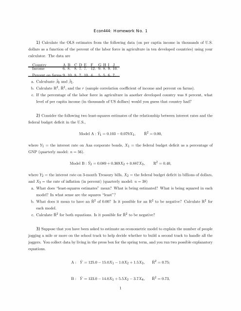
1) <strong>Calculate</strong> <strong>the</strong> <strong>OLS</strong> <strong>estimates</strong> <strong>from</strong> <strong>the</strong> following data (on per captia income in thousands of U.S.<br />
dollars as a function of <strong>the</strong> percent of <strong>the</strong> labor force in agriculture in ten developed countries) using your<br />
calculator. The data are<br />
Country A B C D E F G H I J<br />
Income 6. 8. 8. 7. 7. 12. 9. 8. 9. 10.<br />
Percent on farms 9. 10. 8. 7. 10. 4. 5. 5. 6. 7.<br />
a. Calculuate ˆβ 0 and ˆβ 1 .<br />
b. <strong>Calculate</strong> R 2 , ¯R 2 ,and<strong>the</strong>r (sample correlation coefficient of income and percent on farms).<br />
c. If <strong>the</strong> percentage of <strong>the</strong> labor force in agriculture in ano<strong>the</strong>r developed country was 8 percent, what<br />
level of per capita income (in thousands of US dollars) would you guess that country had?<br />
2) Consider <strong>the</strong> following two least-squares <strong>estimates</strong> of <strong>the</strong> relationship between interest rates and <strong>the</strong><br />
federal budget deÞcit in <strong>the</strong> U.S.,<br />
Model A : Ŷ1 =0.103 − 0.079X 1 , ¯R2 =0.00,<br />
where Y 1 = <strong>the</strong> interest rate on Aaa corporate bonds, X 1 = <strong>the</strong> federal budget deÞcit as a percentage of<br />
GNP (quarterly model: n =56).<br />
Model B : Ŷ2 =0.089 + 0.369X 2 +0.887X 3 , R 2 =0.40,<br />
where Y 2 = <strong>the</strong> interest rate on 3-month Treasury bills, X 2 = <strong>the</strong> federal budget deÞcit in billions of dollars,<br />
and X 3 =<strong>the</strong>rateofinßation (in percent) (quarterly model: n =38)<br />
a. What does “least-squares <strong>estimates</strong>” mean? What is being estimated? What is being squared in each<br />
model? In what sense are <strong>the</strong> squares “least”?<br />
b. What does it mean to have an ¯R 2 of 0.00? Is it possible for an R 2 to be negative? <strong>Calculate</strong> R 2 for<br />
each model.<br />
c. <strong>Calculate</strong> ¯R 2 for both equations. Is it possible for ¯R 2 to be negative?<br />
3) Suppose that you have been asked to estimate an econometric model to explain <strong>the</strong> number of people<br />
jogging a mile or more on <strong>the</strong> school track to help decide whe<strong>the</strong>r to build a second track to handle all <strong>the</strong><br />
joggers. You collect data by living in <strong>the</strong> press box for <strong>the</strong> spring term, and you run two possible explanatory<br />
equations.<br />
A: Ŷ =125.0 − 15.0X 1 − 1.0X 2 +1.5X 3 , ¯R2 =0.75;<br />
B: Ŷ =123.0 − 14.0X 1 +5.5X 2 − 3.7X 4 , ¯R2 =0.73,<br />
1
where Y = <strong>the</strong> number of joggers on a given day, X 1 = inches of rain that day, X 2 = hours of sunshine that<br />
day, X 3 = <strong>the</strong> high temperature for that day (in degrees F), X 4 = <strong>the</strong> number of classes with term papers<br />
due <strong>the</strong> next day.<br />
a) Which of <strong>the</strong> two equations do you prefer? Why?<br />
b) How is it possible to get different estimated signs for <strong>the</strong> coefficient of <strong>the</strong> same variable using <strong>the</strong> same<br />
data?<br />
4) David Katz studied faculty salaries as a function of <strong>the</strong>ir “productivity” and estimated a regression<br />
equation with <strong>the</strong> following coefficients:<br />
Ŝ i =11, 155 + 230B i +18A i +102E i +489D i +189Y i + ···,<br />
where S i =<strong>the</strong>salaryof<strong>the</strong>i<strong>the</strong> professor in 1969-70 in dollars per year; B i = <strong>the</strong> number of books published,<br />
lifetime; E i = <strong>the</strong> number of “excellent” articles published, lifetime; D i = <strong>the</strong> number of dissertations<br />
supervised since 1964; and Y i = <strong>the</strong> number of years teaching experience.<br />
a. Do <strong>the</strong> signs of <strong>the</strong> coefficients match your prior expectations?<br />
b. Do<strong>the</strong>relativesizesof<strong>the</strong>coefficients seem reasonable?<br />
c. Suppose a professor had just enough time (after teaching, etc.) to write a book, write two excellent<br />
articles, or supervise three dissertations, which would you recommend? Why?<br />
d. Would you like to reconsider your answer to part b above? Which coefficient seems out of line? What<br />
explanation can you give for that result? Is <strong>the</strong> equation in some sense invalid? Why or why not?<br />
5) Consider <strong>the</strong> least squares estimation of <strong>the</strong> multiple linear regression model:<br />
y i = β 0 + β 1 x 1i + ···+ β k x ki + ² i ,<br />
where i =1, ···,n.Letˆβs be <strong>the</strong> <strong>OLS</strong>E’s, ŷ i = ˆβ 0 + ˆβ 1 x 1i + ···+ ˆβ k x ki and e i = y i − ŷ i be <strong>the</strong> residual.<br />
Show that P n<br />
i=1 (ŷ i − Ȳ )e i =0.<br />
(Hint: use <strong>the</strong> Þrst order conditions for <strong>the</strong> least squares minimization problem which characterizes e i ).<br />
2