(Pure) heteroskedasticity is caused by the error term of a

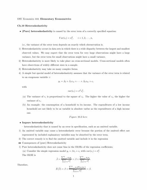
OSU Economics 444: Elementary Econometrics
Ch.10 Heteroskedasticity
• (Pure) heteroskedasticity is caused by the error term of a correctly speciÞed equation:
Var(² i )=σ 2 i ,
i =1, 2, ···,n,
i.e., the variance of the error term depends on exactly which oberservation is.
1) Heteroskedasticity occurs in data sets in which there is a wide disparity between the largest and smallest
observed values. We may expect that the error term for very large observations might have a large
variance, but the error term for small observations might have a small variance.
2) Heteroskedasticity is more likely to take place on cross-sectional models. Cross-sectional models often
have observtions of widely different sizes in a sample.
3) Heteroskedasticity may take on many complex forms.
4) A simple but special model of heteroskedasticity assumes that the variance of the error term is related
to an exogenous variable z:
y i = β 0 + β 1 x 1i + ···+ β k x ki + ² i
with
var(² i )=σ 2 z 2 i .
(a) The variance of ² i is proportional to the square of z i . The higher the value of z i , the higher the
variance of ² i .
(b) An example: the consumption of a household to its income. The expenditures of a low income
household are not likely to be as variable in absolute varlue as the expenditures of a high income
one.
Figure 10.3 here
• Impure heteroskedasticity
— heteroskedasticity that is caused by an error in speciÞcation,suchasanomittedvariable.
1) An omitted variable may cause a heteroskedastic error because the portion of the omitted effect not
represented by included explanatory variables may be absorbed by the error term.
2) The correct remedy is to Þnd the omitted variable and include it in the regression
•• Consequences of (pure) Heteroskedasticity
1) Pure heteroskedasticity does not cause bias in the OLSEs of the regression coefficients.
(a) Consider the simple regression model y i = βx i + ² i with var(² i )=σi 2.
The OLSE is
P n
i=1 ˆβ = x P n
P
iy i
n = β + Pi=1 x i² i
n .
i=1 x2 i
i=1 x2 i
Therefore,
E( ˆβ) =β +
P n
i=1 x iE(² i |x i )
P n
i=1 x2 i
= β.
1

2) The Gauss-Markov theorem does not hold. The OLSE may not be the estimator with the smallest
variance within the class of linear unbiased estimators.
3) The variance formula for the OLSE is not correct. The variance formula tends to underestimate the
true variance of the OLSE.
(a) For the simple regression model y i = βx i + ² i with var(² i )=σi 2 , the true variance of the OLSE ˆβ
is
P n
var(OLS ˆβ) i=1
=
x2 i σ2 i
( P n .
i=1 x2 i )2
(b) The variance formula from the computer (ignoring heteroskedastic variances) is
P n
i=1 e2 i 1
P
n − 1 n
i=1 x2 i
.Itcanbeshownthat
E(
nX
e 2 i )=
i=1
n X
i=1
P n
σi 2 − i=1 x2 i σ2 i
P n
i=1 x2 i
If σi
2 and x2 i are positively correlated, one has
P n P n
i=1 x2 i i=1 σ2 i − P n P n
i=1 x2 i σ2 i
(n − 1)( P i=1
n
≤
x2 i σ2 i
i=1 x2 i )2 ( P n .
i=1 x2 i )2
That is, the expected value of the estimated variance is smaller than the true variance.
•• Testing for Heteroskedasticity
There are many test statistics depending on models. The following are two familiar tests.
• The Park Test
It is designed to test possible heteroskedasticity of the form
var(² i )=σ 2 z δ i .
It has three steps:
1. Obtain the OLS residuals: Estimate the regression model by OLS (ignoring possible heteroskedasticity)
ˆβ and compute
.
e i = y i − ˆβ 0 − ˆβ 1 x 1i − ···− ˆβ k x ki ,
i =1, ···,n.
2. Run thhe regression
ln(e 2 i )=α 0 + α 1 ln(z i )+u i ,
where z i = is a possible (best choice) proportionality factor.
3. Test the signiÞcance of ˆα with a t-test. If it is signiÞcant, this is evidence of heteroskedasticity; otherwise,
not.
4. An empirical example: Woody’s restaurants
OLSE:
ŷ i =102, 192−9075N i +0.355P i +1.288I i
(2053) (0.073) (0.543)
t = − 4.42 4.88 2.37
n =33 ¯R2 =0.579 F =15.65,
2

where
y = the check volume at a Woody’s restaurant
N = the number of nearby competitors
P = the nearby population
I = the average household income of the local area.
Park’ test: try to see if the residuals give any indication of heteroskedasticity by using the population
P — because large error term variances might exist in more heavily populated areas.
ˆ ln(e 2 i )=21.05−0.2865 ln P i
(0.6263)
t = − 0.457
n =33 R 2 =0.0067 F =0.209.
The calculated t-score of -0.457 is too small and there is no strong evidence for heteroskedasticity.
• The White Test
It is more general than the Park test and does not need to decide on possible z factor (as in the Park
test).
1) It runs a regression with the squared residuals on all the original independent variables, their squares
and cross products.
2) For example, for y = β 0 + β 1 x 1 + β 2 x 2 + ², the White’s test regression equation is
e 2 i = α 0 + α 1 x 1i + α 2 x 2i + α 3 x 2 1i + α 4x 2 2i + α 5x 1i x 2i + u i .
3) Test the overall signiÞcance of regression coefficients of the test regression of e 2 i (excluding constant term)
by a F -statistic. Alternatively, use nR 2 ,whereR 2 from the test regression equation, as a chi-square
test with degrees of freedom equal to the number of slope coefficients.
•• Remedies for Heteroskedasticity
• Weighted Least Squares — a version of GLS, specially for the heteroskedastic problem.
The method is to transform the ² i into a new disturbance with constant variance σ 2 .TheOLSapproach
is then applied to the transformed equation. The resulted OLS estimator for the transformed equation is
called the weighted least squares estimator.
1) This approach requires knowledge on the speciÞcation of the variance function.
2) For the model y i = β 0 + β 1 x 1i + ² i where the variance of ² i is speciÞed as
var(² i )=σ 2 x 2 2 .
The transformed equation is
y i
z i
= β 0
1
z i
+ β 1
x 1i
z i
+ u i ,
3

ecause u i = ²i
z i
which is homoskedastic.
a) Estimate the transformed equation by OLS with dependent variable y z
1
z i
and x 1i
z i
.
and explanatory variables
b) Note the transformed equation may not have an intercept term. That is ok.
c) An intercept term may appear if z is one of the explanatory variable x. For example, if z = x 1 ,
then the transformed equation is
y i 1
= β 0 + β 1 + u i ,
x 1i x 1i
where β 1 becomes the intercept term in the transformed equation.
3) The interpretation of the weighted least squares estimates should be the coefficients of the original (not
transformed) regression equation.
4) The weighted least squares is the BLUE (assuming that the variance function) is correctly speciÞed.
• Robust variance estimates for OLSE with an unknown form of heteroskedasticity
1) The OLSE (by ignoring heteroskedastic variances) is unbiased, but the standard variance formula for
the OLSE is valid.
2) This approach is not attempting to get a possible better coefficient estimate. But, it attempts to get a
valid (for large sample) estimate of the proper variance of an OLSE.
3) For example, for the model y i = βx i + ² i (with only a single regressor and no intercept term, for
illustration purpose), the heteroskedasticity-corrected standard errors of OLSE ˆβ is
P n
i=1 x2 i e2 i
( P n ,
i=1 x2 i )2
where e i s are the OLS residuals.
4) The robust variance formula does not require any speciÞcation of the variance function. The technique
works better in large samples.
5) The robust variance can be used in t-tests in hypothesis testing. – use the value of the robust variance
in the denominator of the t ratio formulae.
• RedeÞning the variables
Select variables within theoretical reasoning in the formulation of a regression model which might be
less likely subject to heteroskedasticity.
1) For an example, consider a model of total expenditures (EXP) by governments of different cities that
might be explained by aggregate income (INC), the population (POP), and the average wage (WAGE)
in each city.
A regression model speciÞed as
EXP i = β 0 + β 1 POP i + β 2 INC i + β 3 WAGE i + ² i
might likely have heteroskedastic disturbances because larger cities have larger incomes and large expenditures
thatn the smaller ones.
4

Another theoretical model may be
EXP i
POP i
= α 0 + α 1
INC i
POP i
+ α 2 W AGE i + ² i ,
where the variables are formulated in per capita terms. The large and small size observations disappear
with the per capita variables and this speciÞed equation might be less likely subject to the heteroskedasticity
issue.
• An empirical example:
Try to explain petroleum consumption by state (PCON), using explanatory variables including the size
of the state and gasoline tax rate (TAX).
A possible speciÞcation is
PCON i = β 0 + β 1 REG i + β 2 TAX i + ² i ,
where
PCON i = petroleum consumption in the ith state
REG i = motor vehicle registrations in the ith state
TAX i = the gasoline tax rate in the ith state
1) OLS approach: the estimated equation is
ˆ PCON i =551.7+0.1861REG i − 53.59TAX i
(0.0117) (16.86)
t =15.88 − 3.18
¯R 2 =0.861 n =50.
The estimated coefficients are signiÞcant and have the expected sign.
2) The equation might be subject to heteroskedasticity caused by variation in the size of the states. A plot
of the OLS residuals with respect to REG appear to follow a wider distribution for large values of REG
than for small value of REG.
(Figure 10.8 here)
3) Run a Park test: with ln(REG) asfactor
ˆ ln(e 2 i )=1.650+0.952 ln(REG i)
(0.308)
t =3.09
¯R 2 =0.148 n =50 F =9.533.
The critical t-value for a 1% two-tailed t-test is about 2.7. The computed t =3.09 is larger than 2.7
and, hence, we reject the null hypothesis of homoskedasticity.
5

4) Use robust estimated variances for OLSEs
ˆ PCON i =551.7+0.1861REG i − 53.59TAX i
(0.022) (23.90)
t =8.64 − 2.24
¯R 2 =0.861 n =50.
The robust variances of the OLSEs are larger than those without correction. So the uncorrected variance
formulas underestimate the proper variances of the OLSE.
5) Estimation with the weighted least squares method
PCON ˆ i
1
=218.54 +0.168 − 17.389 TAX i
REG i REG i REG i
(0.014) (4.682)
t =12.27 − 3.71
¯R 2 =0.333 n =50.
The weighted least squares estimates of β 1 and β 2 have smaller (estimated) standard errors than those
of the OLSEs (compared with the robust variances) in 4). The overall Þt is worse but this has no
importance as the dependent variables are different in the two equations.
6) An alternative formulation using per captit petroleum consumption (PCON
POP)
,wherePOP is the population
of a state:
PCON ˆ i
=0.168+0.1082 REG i
− 0.0103TAX i
POP i
POP i
(0.0716) (0.0035)
t =1.51 − 2.95
¯R 2 =0.165 n =50.
This approach is quite different. It is not necessarily better and is not directly comparable to the other
equations. Which specÞcation is better will depend on the purposes of research.
6