Eigenvalues and Eigenvectors
Eigenvalues and Eigenvectors
Eigenvalues and Eigenvectors
You also want an ePaper? Increase the reach of your titles
YUMPU automatically turns print PDFs into web optimized ePapers that Google loves.
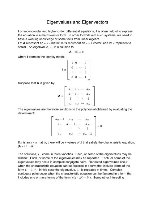
<strong>Eigenvalues</strong> <strong>and</strong> <strong>Eigenvectors</strong><br />
For second-order <strong>and</strong> higher-order differential equations, it is often helpful to express<br />
the equation in a matrix-vector form. In order to work with such systems, we need to<br />
have a working knowledge of some facts from linear algebra.<br />
Let A represent an n n matrix, let x represent an n 1 vector, <strong>and</strong> let represent a<br />
scalar. An eigenvalue, i , is a solution to:<br />
|A − I| 0,<br />
where I denotes the identity matrix:<br />
I ≡<br />
1 0 0<br />
0 1 0<br />
<br />
0 0 1<br />
Suppose that A is given by:<br />
a 11 a 12 a 1n<br />
A ≡<br />
a 21 a 22 a 2n<br />
<br />
a n1 a n2 a nn<br />
The eigenvalues are therefore solutions to the polynomial obtained by evaluating the<br />
determinant:<br />
a 11 − a 12 a 1n<br />
a 21 a 22 − a 2n<br />
<br />
a n1 a n2 a nn − <br />
0<br />
If A is an n n matrix, there will be n values of that satisfy the characteristic equation,<br />
|A − I| 0.<br />
The solutions, i , come in three varieties. Each, or some of the eigenvalues may be<br />
distinct. Each, or some of the eigenvalues may be repeated. Each, or some of the<br />
eigenvalues may occur in complex conjugate pairs. Repeated eigenvalues occur<br />
when the characteristic equation can be factored in a form that include terms of the<br />
form 1 − i m . In this case the eigenvalue, i , is repeated m times. Complex<br />
conjugate pairs occur when the characteristic equation can be factored in a form that<br />
includes one or more terms of the form, a − 2 b 2 . Some other interesting
2<br />
properties of the eigenvalues include that:<br />
1 2 n |A| <strong>and</strong> 1 2 … n traceA<br />
As an example, suppose that n is equal to 2. In this case, the characteristic equation<br />
is given by:<br />
a 11 − a 12<br />
a 21<br />
a 22 − <br />
2 − a 11 a 22 a 11 a 22 − a 12 a 21 0<br />
Define ≡ −a 11 a 22 <strong>and</strong> ≡ a 11 a 22 − a 12 a 21 . The eigenvalues therefore given by:<br />
i − 2 <br />
2<br />
2<br />
− <br />
For each of the n eigenvalues, i , there corresponds an eigenvector, i . <strong>Eigenvectors</strong><br />
satisfy the equation:<br />
A i i i ,or:A − i I i 0<br />
Because A − i , by construction, is singular, there will only be n − 1 independent<br />
equations to solve for the n elements of each of the eigenvectors. <strong>Eigenvectors</strong> give a<br />
direction in n-space, but not a distance in n-space. Consider the case of n 2. In this<br />
case i solves:<br />
a 11 − i a 12 i1<br />
a 21 a 22 − i i2<br />
<br />
0<br />
0<br />
This expression consists of two linear equations, only one of which is independent.<br />
Arbitrarily choose the first of these <strong>and</strong> we find that:<br />
a 11 − i i1 a 12 i2 0, <strong>and</strong> so:<br />
i1<br />
i2<br />
<br />
−a 12<br />
a 11 − i <br />
A convenient normalization is to set 2 i1 2 i2 1.<br />
Systems of Differential Equations<br />
Facts from linear algebra are helpful in solving systems of first-order linear,<br />
homogeneous differential equations. Such systems take the form ẋ Ax, where A<br />
represent an n n matrix, <strong>and</strong> ẋ <strong>and</strong> x represent n 1 vectors. Before engaging in a<br />
study of these more general cases, let us first turn our attention to the case of the<br />
homogeneous second-order differential equation with constant coefficients. That is,<br />
consider:<br />
ÿ aẏ by 0
3<br />
Now consider a change in variables in which we define x 1 ẏ <strong>and</strong> x 2 y. Therefore<br />
ÿ ẋ 1 , ẏ x 1 , <strong>and</strong> y x 2 . We may therefore rewrite the original equation as:<br />
ẋ 1<br />
ẋ 2<br />
<br />
−a −b<br />
1 0<br />
x 1<br />
x 2<br />
Let us guess a solution to the original differential equation that takes the form:<br />
yt ce t<br />
Now take the derivatives of this solution, ẏ ce t <strong>and</strong> ÿ c 2 e t . Now plug these<br />
expressions back into the original differential equation to obtain:<br />
c 2 e t ace t bce t 2 a bce t 0,<br />
if <strong>and</strong> only if 2 a b 0, forc ≠ 0, e t ≠ 0.<br />
The solutions to the polynomial equation, 2 a b 0, are identical to the<br />
eigenvalues of the matrix A. That is:<br />
|A − I| <br />
−a − −b<br />
1 −<br />
2 a b 0<br />
In this, a 2 2 case, there are two eigenvalues, 1 <strong>and</strong> 2 . The solution therefore<br />
takes the form:<br />
ẏ<br />
y<br />
<br />
x 1<br />
x 2<br />
<br />
c 11 e 1t c 12 e 2t<br />
c 21 e 1t c 22 e 2t<br />
We are primarily interested in the solution for yt, which is given by:<br />
yt c 21 e 1t c 22 e 2t<br />
The constants c 21 <strong>and</strong> c 22 are determined from the initial conditions. Once we find c 21<br />
<strong>and</strong> c 22 , it is straightforward to solve for c 11 <strong>and</strong> c 12 .<br />
Let us next consider how to deal with solutions to the generalized homogeneous<br />
system of two differential equations.<br />
ẋ Ax <br />
a 11 a 12<br />
a 21 a 22<br />
x.<br />
So far, we are dealing with 2 2 systems, but the techniques you are learning here<br />
generalize to systems in higher dimensions. Systems of differential equations come<br />
up all the time in economics; the classic example in macroeconomic theory is the<br />
model of optimal growth in which both consumption <strong>and</strong> capital stock are determined<br />
simultaneously by the savings decision of the representative household. Thus this<br />
discussion is not an arid exercise in linear algebra, differential equations, <strong>and</strong> complex
4<br />
variables. Instead it constitutes the bread <strong>and</strong> butter of a lot of modern<br />
macroeconomics.<br />
It should not be not surprising to you now that the cases of interest are essentially a<br />
taxonomy of the characteristic equation p a 11 − a 22 − − a 21 a 12 . There are<br />
four cases: (1) 1 2 0; (2) both roots are real; (3) the two roots are complex<br />
conjugates; <strong>and</strong> (4) 1 2 ≠ 0, in which the roots are the same real number.<br />
Let’s dispose of the first case immediately. If 1 2 0, then either A <br />
0 0<br />
0 0<br />
0 a 12<br />
0 0<br />
or A <br />
or A <br />
. If any of these is true, then we are not<br />
0 0<br />
a 21 0<br />
dealing with a system of differential equations because either one or both variables is<br />
stationary <strong>and</strong> no variable’s rate of change depends upon its own value.<br />
If A <br />
0 0<br />
0 0<br />
, then xt x0.<br />
If A <br />
0 a 12<br />
0 0<br />
, then xt <br />
x 1 0 a 12 x 2 0t<br />
x 2 0<br />
.<br />
If A <br />
0 0<br />
a 21 0<br />
, then xt <br />
x 1 0<br />
x 2 0 a 21 x 1 0t<br />
,<br />
where x0 <br />
x 1 0<br />
x 2 0<br />
is given.<br />
The second case is not so trivial. Let 1 ≠ 2 both be real. Let M be the matrix whose<br />
columns are the two eigenvectors for 1 , <strong>and</strong> 2 .Since<br />
AM M M 1 0<br />
, we know that M −1 AM. As long as M is non-singular,<br />
0 2<br />
M −1 exists. For distinct eigenvalues, ( 1 ≠ 2 ), M is always non-singular.<br />
Now we do a nifty change of coordinates. Write x My <strong>and</strong> note that y M −1 x.<br />
Then ẋ Mẏ since the M matrix is a matrix of constants. Hence we can rewrite our<br />
system as Mẏ ẋ Ax AMy <strong>and</strong> thus<br />
ẏ M −1 AMy y.
5<br />
y 1 0exp 1 t<br />
But the solution to this equation is just yt <br />
. We are only<br />
y 2 0exp 2 t<br />
halfway there because this solution is in the wrong basis; we have to get rid of the<br />
change of coordinates. In particular, we typically know x0, not y0. Recalling that<br />
x My, we can write y0 M −1 x0. So that pins down the initial condition in the<br />
changed coordinates. But also xt Myt M<br />
answer.<br />
y 10exp 1 t<br />
y 2 0exp 2 t<br />
, <strong>and</strong> that is our<br />
To make things concrete, always follow these exact steps. First, calculate the<br />
eigenvalues <strong>and</strong> some corresponding eigenvectors. Second write the matrix whose<br />
columns are the eigenvectors <strong>and</strong> invert it. Third, use this inverse <strong>and</strong> your<br />
knowledge about the initial conditions to figure out y0. Fourth, use y0 <strong>and</strong> the<br />
matrix whose columns are the eigenvectors to get your answer in the original basis.<br />
5 3<br />
1<br />
Here is an example. Let A <br />
with x0 . Then 1 2 <strong>and</strong><br />
−6 −4<br />
1<br />
2 −1 are eigenvalues, <strong>and</strong> the matrix whose columns are the corresponding<br />
eigenvectors is M <br />
1 −1<br />
−1 2<br />
. The inverse of this matrix is M −1 <br />
2 1<br />
1 1<br />
. So<br />
the initial condition in the changed coordinates is y0 <br />
2 1<br />
1 1<br />
1<br />
1<br />
<br />
3<br />
2<br />
.<br />
Hence the solution in the changed basis is yt <br />
to our original problem is<br />
3exp2t<br />
2exp−t<br />
. Finally, the solution<br />
xt Myt <br />
1 −1<br />
−1 2<br />
3exp2t<br />
2exp−t<br />
<br />
3exp2t − 2exp−t<br />
−3exp2t 4exp−t<br />
.<br />
Check that this is the right answer.<br />
We may also write a simple set of Matlab comm<strong>and</strong>s to perform the diagonalization<br />
procedure. This procedure also works for higher-order linear systems. The set of<br />
comm<strong>and</strong>s is given below.<br />
A[..]: Square matrix<br />
[M,lambda]eig(A)
6<br />
tsym(’t’)<br />
zexp(diag(lambda)*t)<br />
x0[..]: column vector of initial conditions<br />
y0inv(M)*x0<br />
yy0.*z<br />
xM*y<br />
The third case occurs when the two roots are complex conjugates. The st<strong>and</strong>ard<br />
diagonalization procedure still works. The eigenvectors also occur in conjugate pairs.<br />
Much of the solution process involves working with complex vectors <strong>and</strong> matrices.<br />
Operations like computing the inverse of a matrix work with complex values as well as<br />
simple real numbers. However, when the process concludes, we obtain a real valued<br />
time function for the solution. Unfortunately, this procedure can give results which are<br />
not easy to interpret. To see this, try using the suggested Matlab technique for solving<br />
a 2 2 system with complex roots. It may appear that the time functions in the<br />
solution are complex. In fact, this is not the case.<br />
An alternate solution technique separates out the real <strong>and</strong> imaginary parts of the<br />
eigenvalues <strong>and</strong> eigenvectors <strong>and</strong> performs an essentially idetical set of steps. For<br />
complex conjugate eigenvalues, can write 1 a bi <strong>and</strong> 2 a − bi with b 0. We<br />
are going to do a very similar process now, but we shall endeavour to write<br />
A MT a,b M −1 a −b<br />
where T a,b <br />
is the canonical (anti-clockwise) ”twisting”<br />
b a<br />
matrix. Of course, if we find a clever change of coordinates <strong>and</strong> write x My, then<br />
ẋ Ax will be equivalent to ẏ M −1 AMy T a,b y.<br />
HowdowefindtheM matrix? Just solve for a complex-valued eigenvector that<br />
corresponds to the eigenvalue 1 a bi. Such an eigenvector can always be written<br />
in the form z i<br />
m 11<br />
m 21<br />
<br />
m 12<br />
m 22<br />
<strong>and</strong> then the matrix we are looking for is<br />
m 11 m 12<br />
M <br />
. Pay attention to the order of the columns. The reason that we<br />
m 21 m 22<br />
put the imaginary part in the first column is that the definition of any eigenvector is<br />
A z 1 1 z 1<br />
<br />
where all these numbers can be complex. Since these are<br />
z 2 1 z 2<br />
complex numbers. this equation is equivalent to:
7<br />
A im 11<br />
im 12<br />
m 12<br />
m 22<br />
<br />
im 11<br />
im 12<br />
m 12<br />
m 22<br />
T a,b ,<br />
where the first column on each side keeps track of the imaginary part <strong>and</strong> the second<br />
column keeps track of the real part. Thus T a,b M −1 AM. The matrix M will have an<br />
inverse because the imaginary roots of the characteristic equation come in pairs. So<br />
this change of coordinates allows us to write the original equation ẋ Ax as<br />
ẏ M −1 ẋ M −1 Ax M −1 AMy T a,b y. From our knowledge about complex<br />
variables, we know that:<br />
y 1 t<br />
y 2 t<br />
expat<br />
ucostb − vsintb<br />
usintb vcostb<br />
,<br />
for given initial conditions<br />
y 1 0<br />
y 2 0<br />
<br />
u<br />
v<br />
.<br />
Again, we can always compute y0 M −1 x0 because x0 is what we were really<br />
given. Then<br />
xt M<br />
expaty 10costb − y 2 0sintb<br />
expaty 1 0sintb y 2 0costb<br />
is the answer to the initial value problem.<br />
0 −2<br />
1<br />
Here is another example. Let A <br />
with x0 . Then 1 1 i<br />
1 2<br />
1<br />
<strong>and</strong> 2 1 − i are the eigenvalues. So we already know that our canonical twisting<br />
1 −1<br />
matrix will be T a,b <br />
. Now we need to compute an eigenvector<br />
1 1<br />
corresponding to 1 1 i. (Always pick the one with the positive imaginary part.)<br />
Using the definition of an eigenvector, we have<br />
A − 1 Iz <br />
−1 − i −2<br />
1 1 − i<br />
z 1<br />
z 2<br />
<br />
0<br />
0<br />
.<br />
(It may not be obvious, but the top <strong>and</strong> bottom rows give the same information; you<br />
can check this by computing 2/−1 − i. The bottom row tells us that an easy<br />
eigenvector is:<br />
z 1<br />
z 2<br />
<br />
1 − i<br />
−1<br />
i<br />
−1<br />
0<br />
<br />
1<br />
−1<br />
.
8<br />
Then the matrix giving the change of coordinates is M <br />
−1 1<br />
0 −1<br />
. The inverse of<br />
this matrix is M −1 <br />
−1 −1<br />
0 −1<br />
. This means that we wan rewrite ẋ Ax as:<br />
ẏ <br />
−1 −1<br />
0 −1<br />
0 −2<br />
1 2<br />
−1 1<br />
0 −1<br />
y <br />
1 −1<br />
1 1<br />
y.<br />
Also, the initial condition in the changed coordinates is:<br />
y0 <br />
−1 −1<br />
0 −1<br />
1<br />
1<br />
<br />
−2<br />
−1<br />
.<br />
The solution in the changed basis is:<br />
yt expt<br />
−2cost sint<br />
−2sint − cost<br />
.<br />
Finally, the solution to our original problem is<br />
xt Myt expt<br />
−1 1<br />
0 −1<br />
−2cost sint<br />
−2sint − cost<br />
expt<br />
cost − 3sint<br />
cost 2sint<br />
.<br />
Again, check that this is the right answer.<br />
We may also write a somewhat complicated Matlab routine which follows these same<br />
steps. Try the procedure outlined as follows:<br />
A[ ]<br />
x0[ ]<br />
[M lambda]eig(A)<br />
[C I]max(imag(lambda))<br />
bM(:,I(1))<br />
b2real(b)<br />
b1imag(b)<br />
M[b1’;b2’]’<br />
y0inv(M)*x0<br />
areal(lambda(1,1))<br />
bmax(max(imag(lambda)))<br />
y1sym(’y1’)<br />
y2sym(’y2’)
9<br />
tsym(’t’)<br />
uy0(1)<br />
vy0(2)<br />
y1exp(a*t)*(u*cos(b*t)-v*sin(b*t))<br />
y2exp(a*t)*(v*cos(b*t)u*sin(b*t))<br />
y[y1;y2]<br />
xM*y<br />
xsimplify(x)<br />
The fourth <strong>and</strong> final case occurs when A has two identical (real) roots that are not<br />
zero. Write 1 2 ≠ 0. There are two possibilities. First, if A I, then the<br />
differential equation is already uncoupled, <strong>and</strong> we can solve it immediately. If A ≠ I,<br />
then you can write N A − I where N 2 0 0<br />
<br />
. Then the general solution to<br />
0 0<br />
ẋ Ax canbewrittenasxt exptI tN, <strong>and</strong> the definite solution is<br />
x 1 0<br />
xt exptI tN<br />
. (Explaining why these facts are true is beyond the<br />
x 2 0<br />
scope of this course. They are based on a Taylor series expansion for operators on<br />
matrices.)<br />
1 −1<br />
1<br />
Our final example will be A <br />
with x0 . The characteristic<br />
1 3<br />
1<br />
equation has 1 − 3 − 1 0, <strong>and</strong> thus 2 − 4 4 − 2 2 0. Sothereare<br />
two identical roots. Now we write N A − 2I <br />
N 2 0.) We may conclude that:<br />
−1 −1<br />
1 1<br />
. (Make sure that<br />
xt exp2tI tN<br />
x 1 0<br />
x 2 0<br />
exp2t<br />
1 − 2t<br />
1 2t<br />
.<br />
Finally, check that this is the right answer.


