Chapter on Discrete Choice Models Linear Probability Model ...
Chapter on Discrete Choice Models Linear Probability Model ...
Chapter on Discrete Choice Models Linear Probability Model ...
Create successful ePaper yourself
Turn your PDF publications into a flip-book with our unique Google optimized e-Paper software.
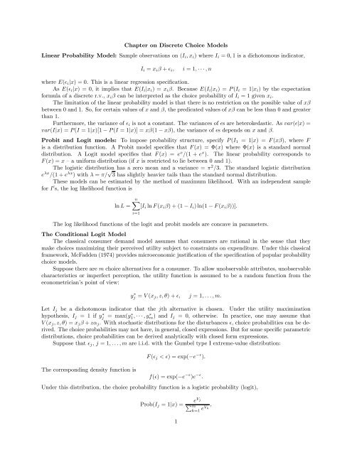
<str<strong>on</strong>g>Chapter</str<strong>on</strong>g> <strong>on</strong> <strong>Discrete</strong> <strong>Choice</strong> <strong><strong>Model</strong>s</strong><br />
<strong>Linear</strong> <strong>Probability</strong> <strong>Model</strong>: Sample observati<strong>on</strong>s <strong>on</strong> (I i ,x i )whereI i =0, 1 is a dichotomous indicator,<br />
I i = x i β + ² i ,<br />
i =1, ···,n<br />
where E(² i |x) = 0. This is a linear regressi<strong>on</strong> speciÞcati<strong>on</strong>.<br />
As E(² i |x) = 0, it implies that E(I i |x i )=x i β. Because E(I i |x i )=P (I i =1|x i ) by the expectati<strong>on</strong><br />
formula of a discrete r.v., x i β can be interpreted as the choice probability of I i =1givenx i .<br />
The limitati<strong>on</strong> of the linear probability model is that there is no restricti<strong>on</strong> <strong>on</strong> the possible value of xβ<br />
between 0 and 1. So, for certain values of x and β, the predicated values of xβ can be less than 0 and greater<br />
than 1.<br />
Furthermore, the variance of ² i is not a c<strong>on</strong>stant. The variances of ²s areheterokedastic. Asvar(²|x) =<br />
var(I|x) =P (I =1|x)[1 − P (I =1|x)] = xβ(1 − xβ), the variance of ²s depends <strong>on</strong> x and β.<br />
Probit and Logit models: To impose probability structure, specify P (I 1 =1|x) =F (xβ), where F<br />
is a distributi<strong>on</strong> functi<strong>on</strong>. A Probit model speciÞes that F (x) =Φ(x) whereΦ(x) is a standard normal<br />
distributi<strong>on</strong>. A Logit model speciÞes that F (x) = e x /(1 + e x ). The linear probability corresp<strong>on</strong>ds to<br />
F (x) =x — a uniform distributi<strong>on</strong> (if x is restricted to lie between 0 and 1).<br />
The logistic distributi<strong>on</strong> has a zero mean and a variance = π 2 /3. The standard logistic distributi<strong>on</strong><br />
e λx /(1 + e λx )withλ = π/ √ 3 has slightly heavier tails than the standard normal distributi<strong>on</strong>.<br />
These models can be estimated by the method of maximum likelihood. With an independent sample<br />
for I 0 s, the log likelihood functi<strong>on</strong> is<br />
ln L =<br />
nX<br />
[I i ln F (x i β)+(1− I i )ln(1− F (x i β))].<br />
i=1<br />
The log likelihood functi<strong>on</strong>s of the logit and probit models are c<strong>on</strong>cave in parameters.<br />
The C<strong>on</strong>diti<strong>on</strong>al Logit <strong>Model</strong><br />
The classical c<strong>on</strong>sumer demand model assumes that c<strong>on</strong>sumers are rati<strong>on</strong>al in the sense that they<br />
make choices maximizing their perceived utility subject to c<strong>on</strong>straints <strong>on</strong> expenditure. Under this classical<br />
framework, McFadden (1974) provides microec<strong>on</strong>omic justiÞcati<strong>on</strong> of the speciÞcati<strong>on</strong> of popular probability<br />
choice models.<br />
Suppose there are m choice alternatives for a c<strong>on</strong>sumer. To allow unobservable attributes, unobservable<br />
characteristics or imperfect percepti<strong>on</strong>, the utility functi<strong>on</strong> is assumed to be a random functi<strong>on</strong> from the<br />
ec<strong>on</strong>ometrician’s point of view:<br />
y ∗ j = V (x j,z,θ)+²,<br />
j =1,...,m.<br />
Let I j be a dichotomous indicator that the jth alternative is chosen. Under the utility maximizati<strong>on</strong><br />
hypothesis, I j =1ify ∗ j = max(y ∗ 1 , ···,y∗ m)andI j = 0, otherwise. In practice, <strong>on</strong>e may assume that<br />
V (x j ,z,θ) =x j β + zα j . With stochastic distributi<strong>on</strong>s for the disturbances ², choice probabilities can be derived.<br />
The choice probabilities may not have, in general, closed expressi<strong>on</strong>s. But for some speciÞc parametric<br />
distributi<strong>on</strong>s, choice probabilities can be derived analytically with closed form expressi<strong>on</strong>s.<br />
Suppose that ² j , j =1,...,m are i.i.d. with the Gumbel type I extreme-value distributi<strong>on</strong>:<br />
The corresp<strong>on</strong>ding density functi<strong>on</strong> is<br />
F (² j
where V j denotes V (x j ,z) for simplicity. This can be shown as follows. Since yj ∗ =max(y∗ 1 , ···,y∗ m )is<br />
equivalent to ² k
The Hessian matrix is n<strong>on</strong>-positive deÞnite and the log likelihood functi<strong>on</strong> is c<strong>on</strong>cave.<br />
The c<strong>on</strong>diti<strong>on</strong>al logit model has a restrictive property known as the independence of irrelevant alternative<br />
property (IIA): The probability odds ratio for the jth and the kth choices is the same irrespective of the<br />
total number m of choices. This is so, because<br />
Prob(I j =1|{1, 2,...,m})<br />
Prob(I k =1|{1, 2,...,m}) = eV j<br />
e V k<br />
= Prob(I j =1|{j, k})<br />
Prob(I k =1|{j, k}) .<br />
The IIA property is inappropriate for some situati<strong>on</strong>s. An example is the so-called blue bus and red bus<br />
paradox. Suppose that each c<strong>on</strong>sumer has three alternatives in choosing the red bus, the blue bus or<br />
his/her own automobile to work. Let x 1 (red bus), x 2 (blue bus) and x 3 (car) be the attributes of the<br />
three transportati<strong>on</strong> modes. Suppose that c<strong>on</strong>sumers treat the two buses indifferent and are also indifferent<br />
between the automobile mode and the bus mode. In such situati<strong>on</strong>, Prob(I 1 =1|x 1 ,x 2 )=Prob(I 1 =<br />
1|x 1 ,x 3 )=Prob(I 2 =1|x 2 ,x 3 )=1/2 andProb(I 1 =1|x 1 ,x 2 ,x 3 )=Prob(I 2 =1|x 1 ,x 2 ,x 3 )=1/4. It<br />
follows that Prob(I1=1|x1,x2,x3)<br />
Prob(I1=1|x1,x3)<br />
Prob(I 3=1|x 1,x 2,x 3)<br />
=1/2 and<br />
Prob(I 3=1|x 1,x 3)<br />
=1. TheIIApropertyisnotsatisÞed in this<br />
situati<strong>on</strong>. The inc<strong>on</strong>sistency occurs because the two bus modes are perceived as similar alternatives rather<br />
than independent alternatives by the individual.<br />
3


